A Cutting-plane Method for Semidefinite Programming
with Potential Applications on Noisy Quantum Devices

Abstract

There is an increasing interest in quantum algorithms for optimization problems. Within convex optimization, interior-point methods and other recently proposed quantum algorithms are non-trivial to implement on noisy quantum devices. Here, we discuss how to utilize an alternative approach to convex optimization, in general, and semidefinite programming (SDP), in particular. This approach is based on a randomized variant of the cutting-plane method. We show how to leverage quantum speed-up of an eigensolver in speeding up an SDP solver utilizing the cutting-plane method. For the first time, we demonstrate a practical implementation of a randomized variant of the cutting-plane method for semidefinite programming on instances from SDPLIB, a well-known benchmark. Furthermore, we show that the RCP method is very robust to noise in the boundary oracle, which may make RCP suitable for use even on noisy quantum devices.

I Introduction

Considering that gate-based quantum computers are expected to aid in solving specific optimization problems across many domains, including quantum chemistry Ganzhorn et al. (2019), machine learning Havlicek et al. (2019), and computational finance Egger et al. (2020), it may seem natural to seek quantum algorithms for convex optimization. Quantum speedup in convex optimization seems elusive, in general. Garg et al. Garg et al. (2021) have shown that in optimizing a Lipschitz-continuous, but otherwise arbitrary convex function over the unit ball, first-order methods Garg et al. (2021) have no quantum speedup over gradient descent, when restricted to the black-box access to the values and gradients of the convex function. One should hence consider other special cases, preferably as broad as possible, and possibly avoiding the black-box access.

Semidefinite programming (SDP) is a broad special case of convex optimization, which has attracted a substantial recent interest. Initially, Brandao and Svore (2017); Van Apeldoorn et al. (2017); Brandão et al. (2019); van Apeldoorn and Gilyén (2019) “quantized” the so-called multiplicative-weight-update (MWU) algorithm of Arora and Kale Arora and Kale (2007) and its variants by Hazan Hazan (2008). Subsequently, Kerenidis and Prakash (2020); Augustino et al. (2021) attempted a translation of primal-dual interior-point methods Wright (1997) to quantum computers. Finally, in Gilyén et al. (2019); Van Apeldoorn et al. (2020); Chakrabarti et al. (2020), the authors study the relationship of several oracles useful in first-order algorithms, but do not claim a run-time of a particular algorithm for SDPs. These results are summarized in Table 1. While some of the quantum algorithms Brandão et al. (2019) are reported as scaling with $O(\sqrt{m}\ \textrm{poly}(\log(m),\log n))$ Brandão et al. (2019) for $m$ constraints in $n\times n$ matrices, this requires the diameter of the convex set to be independent of the dimension, while the dependence is quadratic, in general. Furthermore, none of these algorithms have been implemented in an actual quantum device, or its simulator.

Here, we consider another method for solving SDPs, which can be run in part on the quantum computer. In particular, we “quantize” the so-called randomized cutting plane (RCP) method. The cutting-plane methods Grötschel et al. (2012) have produced a variety of classical theoretical guarantees, as surveyed in Table 2, including the first polynomial-time algorithm for linear programming, but yielded little in terms of practical implementations in classical computers. This is because a certain sub-routine, known as the boundary oracle, is classically almost as demanding as the original problem. We show how to leverage quantum speed-up of an eigensolver in speeding up the RCP method. Furthermore, we demonstrate an implementation of the RCP method, which is very robust to noise in the boundary oracle. The robustness to noise may make RCP suitable for use even on noisy quantum devices, which are available within the foreseeable future.

We formalize the problem and discuss the related work in more detail in Sec. II. We present our main result in Sec. III. Finally, we discuss our numerical results in Sec. IV.

Table 1: An overview of recently proposed quantum algorithms for convex optimization on quantum computers, sorted by their appearance in arxiv (listed under Year). In the upper bounds, we drop polylogarithmic terms.

Reference	Year	Algorithm	Complexity	Complexity ref.
Brandao and Svore (2017)	2016	Multiplicative weights update	$\sqrt{mn}s^{2}(Rr/\epsilon)^{32}$	Cor. 17
Van Apeldoorn et al. (2017); Van Apeldoorn et al. (2020); van Apeldoorn (2020)	2017	Multiplicative weights update	$\sqrt{mn}s^{2}(Rr/\epsilon)^{8}$	Thm. 1 of Van Apeldoorn et al. (2020)
Brandão et al. (2019)	2017	Multiplicative weights update	$(\sqrt{m}/\epsilon^{10}+\sqrt{n}/\epsilon^{12})s^{2}\textrm{poly}(Rr/\epsilon)$	Cor. 6
van Apeldoorn and Gilyén (2019); van Apeldoorn (2020)	2018	Multiplicative weights update	$((\sqrt{m}+\sqrt{n}(Rr/\epsilon))s(Rr/\epsilon)^{4}\approx Rrs(\sqrt{m}/\epsilon^{4}+\sqrt{n}/\epsilon^{5})$	Thm. 17 of van Apeldoorn and Gilyén (2019)
Kerenidis and Prakash (2020)	2018	Interior-point method	$(n^{\omega}+\kappa n^{2}/\delta^{2})\log{1/\epsilon}$, with $\kappa\to\infty$	Cor 7.7
van Apeldoorn et al. (2020)	2018	Subgradient	Not given
Chakrabarti et al. (2020)	2018	Subgradient	Not given
Mohammad Hossein Mohammadi Siahroudi et al. (2021)	2021	Interior-point method	Not given
Augustino et al. (2021)	2021	Interior-point method	$(n^{2.5}/\epsilon+\kappa\delta^{2})$ , with $\kappa\to\infty$	Sec. 5.3
Bharti et al. (2021)	2021	Hybrid, q. preprocessing	Not given

Table 2: A short history of classical algorithms based on the cutting-plane method (focussing on the feasibility). In the upper bounds (listed under Complexity), we drop polylogarithmic terms and let $\rho=nR/\epsilon$.

Ref.	Year	Algorithm	Complexity
Shor (1977); Yudin and Nemirovski (1976); Khachiyan (1980)	1979	Ellipsoid method	$n^{2}\mathcal{S}\log(\rho)+n^{4}\log(\rho)$
Khachiyan et al. (1988); Nesterov and Nemirovskii (1989)	1988	Inscribed ellipsoid	$n\mathcal{S}\log(\rho)+(n\log(\rho))^{4.5}$
Vaidya (1989)	1989	Volumetric center	$n\mathcal{S}\log(\rho)+n^{\omega+1}\log(\rho)$
Atkinson and Vaidya (1995)	1995	Analytic center	$n\mathcal{S}\log^{2}(\rho)+n^{\omega+1}\log^{2}(\rho)+(n\log(\rho))^{2+\omega/2}$
Bertsimas and Vempala (2004)	2004	Random walk	$n\mathcal{S}\log(\rho)+n^{7}\log(\rho)$
Calafiore and Dabbene (2007)	2007	Random walk	probabilistic analyses
Dabbene et al. (2008, 2010)	2010	Random walk	probabilistic analyses
Lee et al. (2015)	2015	Hybrid center	$n\mathcal{S}\log(\rho)+n^{3}\log^{3}(\rho)$
Jiang et al. (2020b)	2019	Volumetric center	$n\mathcal{S}\log(\rho)+n^{3}\log(\rho)$

II Preliminaries and Related Work

II.1 Convex Optimization

We consider a convex constrained optimization problem Boyd and Vandenberghe (2004) of the form

$$\min_{x\in\mathcal{X}}c^{T} x$$ (1)

where $\mathcal{X}\subset\mathbb{R}^{n}$ is a convex compact set with non-empty interior (“convex body”) and $c\in\mathbb{R}^{n}$ defines a linear objective. The linear cost function is taken without loss of generality, since any convex constrained optimization problem can be reduced to this form, . Furthermore, we assume that there exist two Euclidean balls $\mathcal{B}_{r}$ and $\mathcal{B}_{R}$ of radii $0<r<R$, such that $\mathcal{B}_{r}\subseteq\mathcal{X}\subseteq\mathcal{B}_{R}$.

A particularly important class of constrained convex optimization problems are semidefinite programs Anjos and Lasserre (2011):

$$\operatorname{inf}\ \langle C,X\rangle\textrm{ s.t. }\mathcal{A}X=b,X\succeq_{\mathcal{K}}0$$ (SDP)

where cone $\mathcal{K}$ is the cone of positive semidefinite symmetric $n\times n$ matrices $\mathcal{S}_{+}^{n}$, i.e., $\{X=X^{\intercal}\in\mathbb{R}^{n\times n}|\ X\text{ is positive semidefinite}\}$, and $\mathcal{A}\colon\mathcal{S}^{n}\to\mathbb{R}^{m}$ is a linear operator between $\mathcal{S}_{+}^{n}$ and $\mathbb{R}^{m}$:

$$X \mapsto\begin{pmatrix}\langle A_{1},X\rangle\\ \dots\\ \langle A_{m},X\rangle\end{pmatrix}.$$

. This is a proper generalization of linear programming (LP), second-order cone programming (SOCP), and convex cases of quadratically-constrained quadratic programming (QCQP), which underlie much of operations research. SDPs also have extensive applications in combinatorial optimization, control engineering, (quantum) information theory, machine learning Majumdar et al. (2020), and statistics. Under the Unique Games Conjecture Khot et al. (2007); Khot (2010); Khot and Vishnoi (2015), randomized rounding Raghavan and Tompson (1987) of SDPs obtains the best possible polynomial-time classical algorithms for a variety of problems.

Correspondingly, there have been proposed many classical algorithms for solving constrained convex optimization problems. In summary, SDPs can be classically approximated to any precision in polynomial time. Presently, both the best theoretical bounds Jiang et al. (2020a) and the best practical solvers Mosek (2020) employ interior-point methods. At least in theoretical models of computation Blum et al. (2012) where a real-number arithmetic operation can be performed in unit time, there are classical upper bounds Jiang et al. (2020a) on the run time of the form ${\mathcal{\tilde{O}}}(\sqrt{n}(mn^{2}+m^{\omega}+n^{\omega})\log(1/\epsilon))$, where $\mathcal{O}(\cdot)$ indicates the Bachmann–Landau notation, tilde in $\mathcal{\tilde{O}}(\cdot)$ indicates that we drop the polylogarithmic terms, $n$ is the dimension of the problem, $\omega\in[2,2.373)$ is the exponent for matrix multiplication, $m$ is the number of constraints, and nz is the maximal number of non-zero entries per row of the input matrices. For certain smooth instances with sufficient curvature, there are first-order methods Yurtsever et al. (2019), which can be faster still. Nevertheless, many of the instances of SDPs encountered in the real-world that are not possible to solve using classical computers in practice.

To introduce the randomized cutting plane method, it is useful to consider perhaps the single most simple optimization algorithm possible: in each iteration, cut a convex body in two pars at its center of gravity, and repeat with the part that yields better objective function. See Algorithm $1$ for an outline. This is known as the Deterministic Center-of-Gravity (DCG) algorithm and it has been proposed by Levine Levin (1965) and, independently, Newman Newman (1965) in 1965.

II.2 Deterministic Center-of-Gravity (DCG) Algorithm

For a convex body $\mathcal{X}\subset\mathbb{R}^{n}$, define its center of gravity as

$$\operatorname{cg}(\mathcal{X})=\frac{\int_{\mathcal{X}}x\mathrm{d}x}{\int_{\mathcal{X}}\mathrm{d}x}.$$

Algorithm $1$: DCG, cf. Levin (1965); Newman (1965)

Input: $\mathcal{X}$

Output: $z_{k}$

1: $k=0$, $\mathcal{X}_{k}=\mathcal{X}$

2: repeat:

3: $z_{k}=\operatorname{cg}(\mathcal{X}_{k})$

4: $\mathcal{X}_{k+1}=\{x\in\mathcal{X}_{k}:c^{T}(x-z_{k})\leq 0\}$

5: $k=k+1$

6: until a stopping criterion is satisfied.

Proposition 1 (Grünbaum Grünbaum (1960), ).

Let $\mathcal{X}\subset\mathbb{R}^{n}$ be a convex body, and let $x_{G}=cg(\mathcal{X})$ be its center of gravity. Consider any hyperplane $\mathcal{H}=\{x\in\mathbb{R}^{n}:c^{T}(x-x_{G})=0\}$ passing through $x_{G}$. This hyperplane divides the set $\mathcal{X}$ into two subsets

$$\mathcal{X}_{1} =\{x\in\mathcal{X}:c^{T}x>c^{T}x_{G}\},$$

$$\mathcal{X}_{2} =\{x\in\mathcal{X}:c^{T}x\leq c^{T}x_{G}\}.$$

Then, for $i=1,2$:

$$\mbox{vol}(\mathcal{X}_{i})\leq\left(1-\left(\frac{n}{n+1}\right)^{n}\right)\mbox{vol}(\mathcal{X})\leq\left(1-\frac{1}{e}\right)\mbox{vol}(\mathcal{X}).$$ (2)

Remark 2.

Each step of the DCG algorithm guarantees that a given portion of the feasible set is cut out, i.e.,

$$\mbox{vol}(\mathcal{X}_{k+1})\leq\left(1-\frac{1}{e}\right)\mbox{vol}(\mathcal{X}_{k}).$$

Applying this inequality recursively, we obtain the volume inequality

$$\mbox{vol}(\mathcal{X}_{k})\leq\left(1-\frac{1}{e}\right)^{k}\mbox{vol}(\mathcal{X}_{0})\approx(0.63)^{k}\mbox{vol}(\mathcal{X}_{0}),$$ (3)

which proves that DCG has guaranteed geometric convergence in terms of volumes.

By applying Radon’s theorem to the DCG algorithm, we obtain a reduction of cost-function values at each step. Here:

Proposition 3 (Radon, Radon (1921)).

Let $\mathcal{X}\subset\mathbb{R}^{n}$ be a convex body and $x_{G}=cg(\mathcal{X})$ be its center of gravity. Denote by $\mathcal{H}$ an arbitrary $(n-1)$-dimensional hyperplane through $x_{G}$, and let $\mathcal{H}_{1}$ and $\mathcal{H}_{2}$ be the two hyperplane supporting $\mathcal{X}$ and parallel to $\mathcal{H}$. Denote by

$$r(\mathcal{H})=\frac{\min\{\operatorname{dist}(\mathcal{H},\mathcal{H}_{1}),\operatorname{dist}(\mathcal{H},\mathcal{H}_{2})\}}{\max\{\operatorname{dist}(\mathcal{H},\mathcal{H}_{1}),\operatorname{dist}(\mathcal{H},\mathcal{H}_{2})\}}$$

the ratio of the distances from $\mathcal{H}$ to $\mathcal{H}_{1}$ and $\mathcal{H}_{2}$, respectively. Then

$$\min_{\mathcal{H}}r(\mathcal{H})\geq\frac{1}{n}.$$

Specifically:

$$f_{k+1}-f^{*}\leq\frac{n}{n+1}(f_{k}-f^{*}).$$ (2.3)

Indeed, let

$$\mathcal{H}_{1} =\{x\in\mathcal{X}:c^{T}x=c^{T}x_{k}\}$$

$$\mathcal{H} =\{x\in\mathcal{X}:c^{T}x=c^{T}x_{k+1}\}$$

$$\mathcal{H}_{2} =\{x\in\mathcal{X}:c^{T}x=c^{T}x^{*}\},$$

then

$$\operatorname{dist}(\mathcal{H},\mathcal{H}_{1}) =\frac{|c^{T}x_{k}-c^{T}x_{k+1}|}{\mathopen{\|}c\mathclose{\|}}=\frac{c^{T}x_{k}-c^{T}x_{k+1}}{\mathopen{\|}c\mathclose{\|}}$$

$$=\frac{f_{k}-f_{k+1}}{\mathopen{\|}c\mathclose{\|}}$$

and

$$\operatorname{dist}(\mathcal{H},\mathcal{H}_{2})=\frac{f_{k+1}-f^{*}}{\mathopen{\|}c\mathclose{\|}},$$

where we used the fact that $f_{k}\geq f_{k+1}$ and $f_{k+1}\geq f^{*}$. By Radon’s theorem,

$$\frac{f_{k}-f_{k+1}}{f_{k+1}-f^{*}}=\frac{\operatorname{dist}(\mathcal{H},\mathcal{H}_{1})}{\operatorname{dist}(\mathcal{H},\mathcal{H}_{2})}\geq r(\mathcal{H})\geq\min_{\mathcal{H}}r(\mathcal{H})\geq\frac{1}{n},$$

$\Rightarrow$

$$\frac{f_{k}-f_{k+1}}{f_{k+1}-f^{*}}+1\geq\frac{1}{n}+1$$

$\Rightarrow$

$$f_{k+1}-f^{*}\leq\frac{n}{n+1}(f_{k}-f^{*}).$$

Thereby, we obtain the iteration complexity:

Proposition 4 (Rate of convergence of DCG).

Define $D=f_{0}-f^{*}$. Then the DCG algorithm computes an $\alpha$-optimal solution (i.e., such that $f_{k}-f^{*}\leq\alpha$) in a number of steps bounded as

$$k=\left\lceil\frac{\ln\frac{D}{\alpha}}{\ln\frac{n+1}{n}}\right\rceil=\mathcal{O}\left(n\ln\frac{D}{\alpha}\right).$$

This iteration complexity is essentially the same for all cutting-plane methods since 1988, as surveyed in Table 2. We refer to Bubeck (2015) for an in-depth introduction. Notice, however, that computing the deterministic center of gravity (“per-step complexity”) is #P-hard even for 0-1 polytopes Rademacher (2007). One would hence like to consider some alternative sub-routine, while preserving the same rate of convergence.

II.3 An RCP algorithm

Over the past two decades, there have been developed cutting-plane algorithms (Bertsimas and Vempala, 2004; Dabbene et al., 2010, e.g.) that replace the computing of the center of gravity of a convex body with sampling points uniformly at random from the convex body. An outline of such a randomized cutting-plane method is presented in Algorithm $2$.

Table 3: An overview of geometric random walks: Their mixing times and upper bounds on the per-step complexity of sampling uniform distribution over the spectrahedron in the classical implementations by Chalkis et al. Chalkis et al. (2020).

Reference	Year	Random walk	Mixing time	Per-step complexity for SDP
Smith (1984); Lovász (1999)	1984	Hit and Run	Fast Lovász (1999)	$\mathcal{O}(m^{2.697}+m\lg{L}+nm^{2})$
Smith (1984)	1984	Coordinate-directions hit and run	Unknown	$\mathcal{O}(m^{2.697}+m\lg{L}+m^{2})$
Polyak and Gryazina (2014)	2014	Billiard walk	Unknown	$\widetilde{\mathcal{O}}(\rho(m^{2.697}+m\lg{L}+nm^{2}))$
Duane et al. (1987); Mohasel Afshar and Domke (2015); Chevallier et al. (2018)	2015	Hamiltonian Monte Carlo with reflections	Unknown	$\widetilde{\mathcal{O}}(\rho((dm)^{2.697}+md\lg{L}+dnm^{2}))$
Chevallier (2019)	2019	Wang-Landau	Fast Chevallier (2019)	Unknown

Algorithm $2$: Randomized cutting plane Bertsimas and Vempala (2004); Calafiore (2004); Dabbene et al. (2008); Polyak and Shcherbakov (2006)

Input: $\mathcal{X}$

Output: $z_{k}$

1: $k=0$, $\mathcal{X}_{k}=\mathcal{X}$

2: repeat:

3: generate $N_{k}$ uniformly distributed random samples

in $\mathcal{X}_{k}$, $\{x^{(1)},\ldots,x^{(N_{k})}\}$, e.g., using Algorithm $3$

4: $z_{k}=\operatorname*{arg\,min}_{x\in\{x^{(1)},\ldots,x^{(N_{k})}\}}c^{T}x$

5: $\mathcal{X}_{k+1}=\{x\in\mathcal{X}_{k}:c^{T}(x-z_{k})\leq 0\}$

6: $k=k+1$

7: until a stopping rule is satisfied.

The uniform sampling is non-trivial, but a breakthrough result of Lovász and Vempala (2006) showed that it is possible using certain rapidly-mixing geometric random walks Vempala (2005). An overview of the geometric random walks is presented in Table 3. For any such random walk, one needs to provide one or more geometric subroutines, such as the test of membership of a point inside the set, a surface separating a point from the set, etc. Several standard subroutines are beautifully surveyed in Chapter 3 of van Apeldoorn (2020). Our focus in this work will be on the so-called Random Directions Hit and Run random walk Smith (1984), wherein the key subroutine is the intersection of a line (or curve, more generally) with the boundary of the feasible set. This subroutine is commonly known as the boundary oracle (BO). See Algorithm $3$ for an overview.

In the Supplementary Material, we present some background material concerning the statistical properties of the empirical minimum over a convex body in Appendix A. In Appendix B, we present an iteration complexity of the overall procedure, as captured in Algorithm $4$. In particular, we fix minor issues of previous analyses, especially those of Dabbene et al. Dabbene et al. (2008, 2010). In Appendix C, we provide the full pseudo code of the algorithms, specialized to SDPs. We note that the pseudocode and the bounds on the iteration complexity remain the same, independent of whether the boundary oracle is run classically or quantumly.

Algorithm $3$: Hit-and-run (H&R), cf. Smith (1984); Lovász (1999)

Input: $\mathcal{X}$, $x_{0}\in\mathcal{X}$, $M$ (mixing time)

Output: random point $x\in\mathcal{X}$

1: $y^{(0)}=x_{0}$

2: for $i=0$ to $M-1$ do:

3: generate a uniformly distributed random direction $v\in\mathbb{R}^{n}$

4: $\{\underline{x},\bar{x}\}=\texttt{BO}(\mathcal{X},y^{(i)},v)$

5: generate a uniform point $y^{(i+1)}$ in the segment $[\underline{x},\bar{x}]$

6: end for

7: $x=y^{(M)}$

Algorithm $4$: RCP with H&R, cf. Calafiore (2004); Dabbene et al. (2008); Polyak and Shcherbakov (2006)

Input: $\mathcal{X}$, $x_{0}\in\mathcal{X}$, $M$

Output: $z_{k}$

1: $k=0$, $\mathcal{X}_{k}=\mathcal{X}$

2: repeat:

3: for $j=1$ to $N$ do: $x^{(j)}=\texttt{H\&R}(x^{(j-1)},M)$; end for

4: $z_{k}=\min_{x\in\{x^{(1)},\ldots,x^{(N)}\}}c^{T}x$

5: $\mathcal{X}_{k+1}=\{x\in\mathcal{X}_{k}:c^{T}(x-z_{k})\leq 0\}$

6: $k=k+1$

7: until a stopping rule is satisfied.

II.4 Boundary Oracle for Hit-and-Run Walks on the Feasible Set of an SDP

Let us now consider the complexity of implementing a boundary oracle for the Random Directions Hit and Run random walk Smith (1984) for sampling uniformly at random from the spectrahedron (SDP). For convenience, let us consider the dual of the semidefinite program (SDP), also known as the linear matrix inequality (LMI):

$$\min c^{T}x\textrm{ s.t. }F(x) =F_{0}+\sum_{i=1}^{n}x_{i}F_{i}\preceq 0,$$ (LMI)

where $c\in\mathbb{R}^{n}$ and $F_{i}=F_{i}^{T}\in\mathbb{R}^{m\times m}$, $i=0,\ldots,n$, are known symmetric matrices. We then have the convex set

$$\mathcal{X}=\mathcal{X}_{\operatorname{LMI}}=\{x\in\mathbb{R}^{n}:F(x)\preceq 0\}.$$

We assume $\mathcal{X}_{\operatorname{LMI}}$ is nonempty and bounded.

Given $y\in\mathcal{X}_{\operatorname{LMI}}$ such that $F(y)\prec 0$ and a random direction $v\in\mathbb{R}^{n}$, how do we find the intersection points of the line $z=y+\lambda v$ and the boundary of $\mathcal{X}_{k}$ at the $k$-th iteration? First, we have

$$F(y+\lambda v)=F(y)+\lambda(F(v)-F_{0})\triangleq A+\lambda B,\ \lambda\in\mathbb{R}.$$

Next, we obtain the intersection points with the boundary of $\mathcal{X}_{\operatorname{LMI}}$: $\underline{z}=y+\underline{\lambda}v$ and $\bar{z}=y+\bar{\lambda}v$ and test if $\underline{z},\,\bar{z}\in\mathcal{X}_{k}=\{x\in\mathcal{X}_{k-1}:c^{T}(x-z_{k-1})\leq 0\}$. If both points are in $\mathcal{X}_{k}$, then $\{\underline{z},\,\bar{z}\}$ are the intersection points we need. Otherwise, only one of them $\notin\mathcal{X}_{k}$, so w.l.o.g. assume $\bar{z}\notin\mathcal{X}_{k}$, and we need to find the intersection point between the line $z=y+\lambda v$ and the hyperplane $\{x\in\mathcal{X}:c^{T}(x-z_{k-1})=0\}$, which can be easily obtained by solving for $\lambda$ in $c^{T}(y+\lambda v-z_{k-1})=0$. Let $\lambda^{*}$ denote the solution and let $\bar{z}^{\prime}=y+\lambda^{*}v$. Then, $\{\underline{z},\bar{z}^{\prime}\}$ are the desired intersection points.

The work of Calafiore (2004); Dabbene et al. (2008); Polyak and Shcherbakov (2006) can be summarized as follows:

Lemma 5 (Boundary oracle for LMIs, Lemma 6 in Dabbene et al. (2008)).

Let $A\prec 0$ and $B=B^{T}$. Then, the minimal and the maximal values of the parameters $\lambda\in\mathbb{R}$ retaining the negative definiteness of the matrix $A+\lambda B$ are given by

$$\underline{\lambda}=\left\{\begin{array}[]{lr}\max\limits_{\lambda_{i}<0}\lambda_{i}&\\ -\infty&\text{if all}\ \lambda_{i}>0\end{array}\right.$$

and

$$\overline{\lambda}=\left\{\begin{array}[]{lr}\min\limits_{\lambda_{i}>0}\lambda_{i}&\\ +\infty&\text{if all}\ \lambda_{i}<0,\end{array}\right.$$

where $\lambda_{i}$ are the generalized eigenvalues of the pair of matrices $(A,-B)$, i.e., $Av_{i}=-\lambda_{i}Bv_{i}$.

The semidefinite generalized eigenvalue problem (Lucas, 2004, Chapter 3) could be seen as a special cases of the polynomial eigenvalue problem Tisseur (2000); Guettel and Tisseur (2017). There, we wish to compute $\lambda\in\mathbb{R}$ and $x\in\mathbb{R}^{m}$ satisfying

$$(B_{d}\lambda^{d}+\cdots+B_{1}\lambda+B_{0})x=0\enspace,$$ (PEP)

where $B_{i}\in\mathbb{R}^{m\times m}$ are matrices, out of which $B_{d}$ and $B_{0}$ are invertible, and all could be seen as coefficients of a univariate matrix polynomial.

Despite much recent progress in computational approach to the polynomial eigenvalue problem Tisseur (2000); Berhanu (2005); Armentano and Beltran (2019); Beltrán and Kozhasov (2019), and effective computational geometry for surfaces Boissonnat and Teillaud (2006) more broadly, a classical implementation of the boundary oracle that would make the hit-and-run walk on the feasible set of SDP (or LMI) is still lacking. In particular, the present best classical run-time bound is:

Lemma 6 (Chalkis et al., Chalkis et al. (2020)).

Consider a PEP of degree $d$, involving matrices of dimension $m\times m$, with integer elements of bitsize at most $\tau$. There is a randomized algorithm for computing the eigenvalues and the eigenvectors of PEP up to precision $\epsilon=2^{-L}$, in time $\widetilde{\mathcal{O}}((md)^{\omega+3}(md)^{3}\tau)$. The arithmetic complexity is $\widetilde{\mathcal{O}}(\delta^{2.697}+md\log(1/\epsilon))$.

Unfortunately, this is not much easier than solving the original convex constrained optimization problem, which has Jiang et al. (2020a) the arithmetic complexity ${\mathcal{\tilde{O}}}(\sqrt{n}(mn^{2}+m^{\omega}+n^{\omega})\log(1/\epsilon))$, and wherein important special cases (van den Brand, 2020, e.g.) can be solved in matrix-multiplication time.

III A Boundary Oracle via Quantum Eigensolvers

Our main result is a family of quantum algorithms for the boundary oracle for hit-and-run walks on the feasible set of an SDP, or rather its dual (LMI). Therein, we transform the generalized eigenvalue problem to an eigenvalue problem on a larger matrix, which makes it possible to use any quantum algorithm for computing the eigenvalues of the larger matrix. Quantum eigensolvers are, in turn, some of the best understood quantum algorithms Kitaev (1995), with practical algorithms (Parker and Joseph, 2020; Egger et al., 2021, e.g.) even for noisy quantum devices. Indeed, one can show Wocjan and Zhang (2006) that any algorithm for a quantum computer with an exponential speed-up is reducible to an eigensolver.

There are two options for linearising the generalized eigenvalue problem, broadly speaking. Either we utilize the companion linearization Gohberg et al. (1982); Mackey et al. (2006); Higham et al. (2006) to transform the polynomial eigenvalue problem (PEP) into a linear pencil in a higher dimension, or we utilize the congruence transformations Lucas (2004). Either way, we express the generalized eigenvalues in the generalized problem as the standard eigenvalues of a larger matrix.

III.1 Companion Linearization

Let us consider the polynomial eigenvalue problem (PEP). Starting from the generalized eigenvalue problem $C_{0}-\lambda C_{1}$, where the companion matrices (Gohberg et al., 1982, Chapter 4) are:

$$C_{0}=\left[\begin{array}[]{cccc}B_{d}&0&\cdots&0\\ 0&I_{m}&\ddots&\vdots\\ \vdots&\ddots&\ddots&0\\ 0&\cdots&0&I_{m}\end{array}\right]\text{, }C_{1}=\left[\begin{array}[]{cccc}B_{d-1}&B_{d-2}&\cdots&B_{0}\\ -I_{m}&0&\cdots&0\\ \vdots&\ddots&\ddots&\vdots\\ 0&\cdots&-I_{m}&0\end{array}\right],$$

where $I_{m}$ denotes the $m\times m$ identity matrix. we obtain the usual linear eigenvalue problem $(\lambda I_{d}-C_{2})z=0$, where

$$C_{2}=\left[\begin{array}[]{cccc}B_{d-1}B_{d}^{-1}&B_{d-2}B_{d}^{-1}&\cdots&B_{0}B_{d}^{-1}\\ -I_{m}&0&\cdots&0\\ \vdots&\ddots&\ddots&\vdots\\ 0&\cdots&-I_{m}&0\end{array}\right].$$

The eigenvectors are roots of the characteristic polynomial of $C_{2}$.

Table 4: A short history of options for translating generalized eigenvalue problems to eigenvalue problems.

Ref.	Year	Approach / Algorithm
Gohberg et al. (1982); Berhanu (2005)	folklore	Companion linearization
Parlett (1971)	1971	Three RRD (SPEC / SPEC / SVD)
Fix and Heiberger (1972)	1972	Three RRD (SPEC / SPEC / QR)
Bunse-Gerstner (1984)	1984	MDR
Cao (1987)	1987	Three RRD (all orthogonal)
Demmel and Kågström (1993)	1993	Generalized Upper Triangular (GUPTRI)
Lucas (2004)	2004	Orthogonal RRD (SPEC / SPEC / SVD)
Lucas (2004)	2004	Non-orthogonal (Cholesky / LDLT / QRP)

This approach is ready to be used on noisy quantum devices, in the sense that it does not require the implementation of any numerical linear algebra on the quantum device, other than the eigensolver, and moreover, in that it is very robust to errors in the quantum eigensolver.

III.2 Congruence Transformations

An alternative approach is known as the congruence transformations. This stems from the work of Lucas (Lucas, 2004, Chapter 3), which generalizes earlier work of Fix and Heiberger Fix and Heiberger (1972), Parlett Parlett (1971), and Cao Cao (1987). We refer to Section 3.4.5 of Lucas (2004) for the discussion of the computational complexity. While this work, summarized in Table 4, is fundamental in (multi)linear algebra, it is surprisingly little known. Having said that, it may be less suited to noisy quantum devices, in the sense that the quantum eigensolver gets compounded up to three times within the quantum boundary oracle.

IV Experimental Results

We have implemented the random-walk variant of the cutting-plane method specialized to SDPs in Python, with a view of inclusion of the code in Qiskit H. Abraham et al. (2019). The pseudo code of the algorithms is presented in Appendix C, while numerical constants and other details of the implementation are discussed in Appendix D.

We have tested our implementation on SDPLIB Borchers (1999), a well-known benchmark. Table 5 presents an overview of the solution quality obtained on a subset of the instances. We should like to stress that the SDPLIB has been designed to test the scalability of classical interior-point methods, and while it may provide the ultimate test of scalability of quantum algorithms for semidefinite programming, none of the quantum algorithms surveyed in Table 1 has been tested on any instances from SDPLIB, yet. Likewise, while there has been much effort focussed on implementations Mittelmann (2003); Chalkis et al. (2020) of SDP solvers, we believe these to be the first reported results of a cutting plane method on the SDPLIB.

As can be seen in Table 5, our method is much slower than classical interior-point methods. For example, on the instance hinf1, which has been originally developed by P. Gahinet within control-theoretic applications, using a $14\times 14$ PSD matrix and 13 inequalities, our method converges to 2 significant digits in the objective function within 127 seconds. In contrast, a commonly-used classical solver SCS 2.1.4 O’Donoghue et al. (2019, 2016) solves the hinf1 to 3 significant digits in the objective function within 5.68 seconds on the same hardware; many interior-point methods Mittelmann (2003) are much faster still. As we detail in Table 6 in Appendix E, on many other instances, our method terminates after 24 hours without obtaining a solution matching 1 significant digit in the value of the objective function. Despite the appealing iteration-complexity results for cutting-plane methods, cf. Table 2, their practical utility remains limited, when executed classically.

In terms of a potential quantum speed-up, much depends on the speed-up of the eigensolver, as discussed in Section III. For instance, on qap6, which features a $37\times 37$ PSD matrix variable, approximately 8 hours and 24 minutes are spent in the eigensolver, classically. A square root of the run-time, which could illustrate a quadratic speed-up in a realistically implementable quantum eigensolver (Somma and Boixo, 2013; Parker and Joseph, 2020, e.g.), would reduce this to less than 174 seconds. A logarithmic reduction of the run-time, which could illustrate the impact of an exponential quantum speed-up , would reduce this to less than 5 seconds. A commonly used classical solver SCS 2.1.4 O’Donoghue et al. (2019, 2016) solves the qap6 within 1.49 seconds on the same classical hardware.

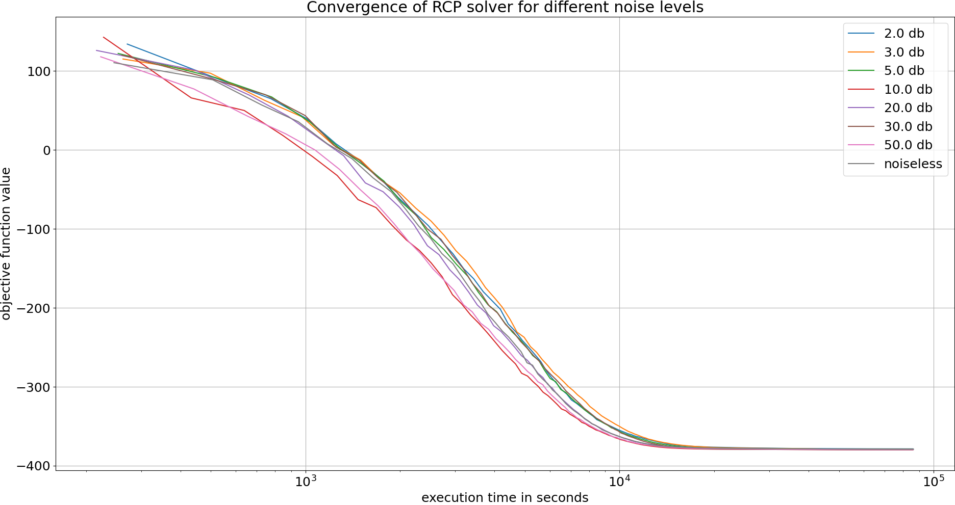
Figure 1: The effect of errors in the eigensolver on the instance qap6, as applied with different signal to noise ratios (SNR). The curves demonstrate the evolution of objective function value in time.

Even the exponential speed-up in the eigensolver would hence yield a speed-up of the overall cutting-plane method only for instances (much) larger than a $37\times 37$ PSD matrix, whilst our current ability to realize any quantum speed-up Lloyd et al. (2014); Parker and Joseph (2020) whatsoever in an eigensolver for an $37\times 37$ matrix is lacking. Indeed, even the state preparation for a $37\times 37$ matrix is presently out of reach. Still, should the state preparation for larger matrices prove feasible, the overall speed-up may be of interest.

On a more positive note, in terms of the robustness to errors in the boundary oracle, which could be implemented with a quantum eigensolver as discussed in Section III, the random-walk variant of the cutting-plane method may be hard to improve upon. As we illustrate in Figure 1, even multiplicative noise in the eigenvalue computation corresponding to the signal-to-noise ratio of approximately 2 dB does not change the performance of the algorithm on qap6, substantially. (See Appendix D for the details of the noise model.) This also has an intuitive interpretation, when one recalls that we use the boundary oracle to estimate the line segment along a sampled random direction that lies within the feasible set. We do not, however, use the estimated end points of the line segment per se: we only sample from the line segment. Unless the error in the eigensolve leads to sampling from beyond the line segment, outside of the feasible set, the error has no discernible impact on the performance and does not propagate further. The fact that we can accommodate a substantial amount of noise in the quantum eigensolver could be seen as a basis of an approach suitable for noisy quantum devices.

Table 5: An overview of the solution quality obtained within a 24-hour time limit on a subset of smaller problems from SDPLIB, a well-known benchmark: Instance name, its variant, number of constraints and size of the matrix variable, reference objective function value in SDPLIB, objective function value obtained by a classical solver (SCS, O’Donoghue et al. (2019, 2016)), and the objective-function value at the termination of RCP (in parentheses, if the run terminated with a time out). Reasons for termination are detailed in Appendix 6.

Instance	Type	$m$	$n\times n$	Ref. Obj.	SCS Obj.	RCP Obj.
hinf1	primal	13	$14\times 14$	2.032600	2.036422	2.253482
hinf10	primal	21	$18\times 18$	108.711800	107.808783	151.069581
mcp100	primal	100	$100\times 100$	226.157350	226.151147	318.123641
mcp124-1	primal	124	$124\times 124$	141.990480	141.988895	(250.149694)
mcp124-2	primal	124	$124\times 124$	269.880170	269.885616	(383.003507)
mcp124-3	primal	124	$124\times 124$	467.750110	467.755324	(614.279456)
mcp124-4	primal	124	$124\times 124$	864.411860	864.413665	(1120.640088)
mcp250-2	primal	250	$250\times 250$	531.930080	531.928325	(758.006964)
mcp250-3	primal	250	$250\times 250$	981.172570	981.185856	(1272.445273)
mcp250-4	primal	250	$250\times 250$	1681.960100	1681.959153	(2155.741152)
truss1	primal	6	$13\times 13$	-8.999996	-8.999996	-7.101001
truss2	primal	58	$133\times 133$	-123.380360	-123.376950	(-21.458773)
truss3	primal	27	$31\times 31$	-9.109996	-9.110169	-5.232127
truss4	primal	12	$19\times 19$	-9.009996	-9.010000	-5.826993

V Conclusions

We have demonstrated how to utilize eigensolvers in solving semidefinite programs, which are perhaps the broadest widely used class of convex optimization problems. The resulting randomized cutting plane method has several non-trivial steps, with several design choices for each step, as documented in Tables  3–4. This may hence suggest something of a framework for the development of further related algorithms, by varying the design choices we made.

Appendix A Statistical properties of the empirical minimum over a convex body

Given $c\in\mathbb{R}^{n}$, we define the following random variables that represent the value of a linear objective evaluated at the random points $x^{(i)}$: $f^{(i)}=c^{T}x^{(i)}$, $i=1,\ldots,N$. Then we can define the so-called empirical minimum over these random points as

$$f_{[1]}=\min_{i=1,\ldots,N}f^{(i)}.$$ (4)

Notice that $f_{[1]}$ is also a random variable; it represents the socalled first order statistics of $f^{(i)}$. The key theorem below proves that, for every convex body $\mathcal{X}$, the expected value of the relative distance between the empirical minimum $f_{[1]}$ and the true one $f^{*}=\min_{\mathcal{X}}c^{T}x$ is bounded from below and from above by constants that depend only on $n$ and $N$.

Lemma 7 (Brunn).

Let $\mathcal{X}\subset\mathbb{R}^{n}$ be a convex body. Define a parallel slice $\mathcal{X}_{s}=\mathcal{X}\cap\{x:x_{1}=s\}$ and its $(n-1)$-dimensional volume $v_{\mathcal{X}}(s)=\mbox{vol}(\mathcal{X}_{s})$. Then the function $v_{\mathcal{X}}(s)^{\frac{1}{n-1}}$ is concave, and

$$\mbox{vol}(\mathcal{X}_{s})^{\frac{1}{n-1}}\geq\lambda\mbox{vol}(\mathcal{X}_{s_{1}})^{\frac{1}{n-1}}+(1-\lambda)\mbox{vol}(\mathcal{X}_{s_{2}})^{\frac{1}{n-1}},$$

where $s=\lambda s_{1}+(1-\lambda)s_{2}$, $\lambda\in[0,1]$.

Proof.

First note that $\lambda\mathcal{X}_{s_{1}}+(1-\lambda)\mathcal{X}_{s_{2}}\subseteq\mathcal{X}_{s}$. Indeed, using convexity of $\mathcal{X}$, for all $(s_{1},\bar{y}_{1})\in\mathcal{X}_{s_{1}}$ and $(s_{2},\bar{y}_{2})\in\mathcal{X}_{s_{2}}$, we have $(s,\bar{y})=(\lambda s_{1}+(1-\lambda)s_{2},\lambda\bar{y}_{1}+(1-\lambda)\bar{y}_{2})=\lambda(s_{1},\bar{y}_{1})+(1-\lambda)(s_{2},\bar{y}_{2})\in\mathcal{X}\cap\{x:x_{1}=s\}=\mathcal{X}_{s}$. Then, by the Brunn-Minkowski inequality, we have

$$\mbox{vol}(\mathcal{X}_{s})^{\frac{1}{n-1}}\geq\mbox{vol}(\lambda\mathcal{X}_{s_{1}}+(1-\lambda)\mathcal{X}_{s_{2}})^{\frac{1}{n-1}}\geq\lambda\mbox{vol}(\mathcal{X}_{s_{1}})^{\frac{1}{n-1}}+(1-\lambda)\mbox{vol}(\mathcal{X}_{s_{2}})^{\frac{1}{n-1}},$$

i.e., $v_{\mathcal{X}}(s)^{\frac{1}{n-1}}$ is concave. ∎

Theorem 8.

Let $\mathcal{X}\subset\mathbb{R}^{n}$ be a convex body. Given $c\in\mathbb{R}^{n}$, define $h=\max_{\mathcal{X}}c^{T}x-\min_{\mathcal{X}}c^{T}x$ and $f^{*}=\min_{\mathcal{X}}c^{T}x$. Then it holds that

$$\frac{h}{nN+1}\leq\mathbb{E}[f_{[1]}-f^{*}] \leq\frac{h}{n}B\left(N+1,\frac{1}{n}\right)$$ (5)

$$\leq h\left(\frac{1}{N+1}\right)^{\frac{1}{n}},$$ (6)

where the expectation is taken with respect to samples $x^{(1\ldots\infty)}$ and $B(\cdot,\cdot)$ is the Euler Beta function.

Proof.

Assume, without loss of generality, that $c=[\,1\,0\ldots 0\,]^{T}$ (that is, $c^{T}x=x_{1}$) and that $x^{*}=\operatorname*{arg\,min}_{\mathcal{X}}c^{T}x=0$. (Indeed, if in general $c^{T}x=\sum_{i=1}^{i=n}c_{i}x_{i}$, then let $y_{1}=\sum_{i=1}^{i=n}c_{i}x_{i}$, so equivalently, we have $\min\tilde{c}^{T}y=y_{1}$, $y\in\tilde{\mathcal{X}}$, where $\tilde{c}=[\,1\,0\ldots 0\,]$ and $\tilde{\mathcal{X}}=\{y\,|\,y_{1}=\sum_{i=1}^{i=n}c_{i}x_{i},\,x\in\mathcal{X}\}$. Notice that $\tilde{\mathcal{X}}$ is still a convex body. If $x^{*}=\operatorname*{arg\,min}_{\mathcal{X}}c^{T}x\neq 0$, then let $y=x-x^{*}$, so equivalently, we have $y^{*}=\operatorname*{arg\,min}_{\{\mathcal{X}-x^{*}\}}c^{T}y=0$.)

We begin by proving the upper bound in (5), following Dabbene et al. (2010), but correcting several flawed steps. Let

$$\mathcal{X}_{s}=\mathcal{X}\cap\{x:x_{1}=s\}$$

Then by Lemma 7, we have

$$\mbox{vol}(\mathcal{X}_{s})^{\frac{1}{n-1}}\geq\lambda\mbox{vol}(\mathcal{X}_{s_{1}})^{\frac{1}{n-1}}+(1-\lambda)\mbox{vol}(\mathcal{X}_{s_{2}})^{\frac{1}{n-1}}$$

for $s=\lambda s_{1}+(1-\lambda)s_{2}$, $\lambda\in[0,1]$. Now define $\mathcal{X}_{0}$ obtained by replacing each $\mathcal{X}_{s}$ by an $(n-1)$-dimensional ball $\mathcal{B}_{s}$ of the same volume and centered at the point $[\,s\,0\ldots 0\,]^{T}$, as shown in Figure 3.1. Then $\mbox{vol}(\mathcal{X}_{0})=\mbox{vol}(\mathcal{X})$ and

$$\mbox{vol}(\mathcal{B}_{s})^{\frac{1}{n-1}}\geq\lambda\mbox{vol}(\mathcal{B}_{s_{1}})^{\frac{1}{n-1}}+(1-\lambda)\mbox{vol}(\mathcal{B}_{s_{2}})^{\frac{1}{n-1}}$$ (7)

Note that the volume of a $n$-dimensional ball $\mathcal{B}$ with radius $r$ is

$$\mbox{vol}(S)=\frac{\pi^{\frac{n}{2}}}{\Gamma(\frac{n}{2}+1)}r^{n},$$

where $\Gamma$ is Euler’s gamma function. Hence, if we denote by $r(s)$ the radius of the $(n-1)$-dimensional ball $\mathcal{B}$ at $s$, then (7) implies that $r(\lambda s_{1}+(1-\lambda)s_{2})\geq\lambda r(s_{1})+(1-\lambda)r(s_{2})$. This, in turn, implies that $r(s)$ is a concave function; thus $\mathcal{X}_{0}$ is a convex set (intuitively, think the shape of $\mathcal{X}_{0}$). Note that now $\mathcal{X}_{0}$ is symmetric about the $x_{1}$ axis.

As a second step, define now the cone $\mathcal{\mathcal{K}}$ with base area $S=\frac{n}{h}\mbox{vol}(\mathcal{X})$, the axis directed along $c$ and located as shown in Figure 3.2, with $h$ being the height of $\mathcal{\mathcal{K}}$. Then, by construction, we have $\mbox{vol}(\mathcal{\mathcal{K}})=\mbox{vol}(\mathcal{X})=\mbox{vol}(\mathcal{X}_{0})$. Let $s^{*}$ be the coordinate at which the sets $\mathcal{X}_{0}$ and $\mathcal{\mathcal{K}}$ intersect; see Figure 3.2. Next, for every $s\in[0,h]$, define the sets $\mathcal{X}^{+}(s)=\{x\in\mathcal{X}:x_{1}\geq s\}$, $\mathcal{X}^{+}_{0}(s)=\{x\in\mathcal{X}_{0}:x_{1}\geq s\}$ and $\mathcal{K}^{+}(s)=\{x\in\mathcal{K}:x_{1}\geq s\}$ as shown in Figure 3.3. Then the following chain of inequalities holds:

$$\mathbb{P}\{f^{(i)}\geq s\} =\mathbb{P}\{x_{1}^{(i)}\geq s\}=\frac{\mbox{vol}(\mathcal{X}^{+}(s))}{\mbox{vol}(\mathcal{X})}=\frac{\mbox{vol}(\mathcal{X}^{+}_{0}(s))}{\mbox{vol}(\mathcal{X}_{0})}$$

$$\leq\frac{\mbox{vol}(\mathcal{K}^{+}(s))}{\mbox{vol}(\mathcal{K})}=1-\frac{\mbox{vol}(\mathcal{K}^{-}(s))}{\mbox{vol}(\mathcal{K})}=1-\left(\frac{s}{h}\right)^{n}=\frac{h^{n}-s^{n}}{h^{n}}$$ (8)

where the last inequality follows from the fact that, for $s\geq s^{*}$,

$$\frac{\mbox{vol}(\mathcal{X}^{+}_{0}(s))}{\mbox{vol}(\mathcal{X}_{0})}\leq\frac{\mbox{vol}(\mathcal{K}^{+}(s))}{\mbox{vol}(\mathcal{K})},$$

and, for $s\leq s^{*}$,

$$\frac{\mbox{vol}(\mathcal{X}^{+}_{0}(s))}{\mbox{vol}(\mathcal{X}_{0})}=1-\frac{\mbox{vol}(\mathcal{X}^{-}_{0}(s))}{\mbox{vol}(\mathcal{X}_{0})}\leq 1-\frac{\mbox{vol}(\mathcal{K}^{-}(s))}{\mbox{vol}(\mathcal{X}_{0})}=\frac{\mbox{vol}(\mathcal{K}^{+}(s))}{\mbox{vol}(\mathcal{K})},$$

where $\mathcal{X}_{0}^{-}(s)=\{x\in\mathcal{X}_{0}:x_{1}<s\}$ and $\mathcal{K}^{-}(s)=\{x\in\mathcal{K}:x_{1}<s\}$.

As a final step for proving the upper bound in (5), notice that $f_{[1]}$ is a positive random variable, and hence we may write

$$\mathbb{E}[f_{[1]}] =\int_{0}^{h}\mathbb{P}\{f_{[1]}\geq s\}\mathrm{d}s=\int_{0}^{h}\left(\mathbb{P}\{f^{(i)}\geq s\}\right)^{N}\mathrm{d}s$$

$$[\text{from}\ (\ref{eq:5})] \leq\int_{0}^{h}\left(\frac{h^{n}-s^{n}}{h^{n}}\right)^{N}\mathrm{d}s$$

$$[t=s^{n}/h^{n}] =\frac{h}{n}\int_{0}^{1}(1-t)^{N}t^{\frac{1}{n}-1}dt=\frac{h}{n}B\left(N+1,\frac{1}{n}\right).$$

Finally, applying Theorem 3.4 in Alzer (2003), we get the following bounds

$$1-\left(\frac{N}{N+1}\right)^{\frac{1}{n}}\leq\frac{1}{n}B\left(N+1,\frac{1}{n}\right)\leq\left(\frac{1}{N+1}\right)^{\frac{1}{n}},$$

thus proving the inequality in (6), with the cone $\mathcal{K}$ being the attainable “worst-case” configuration for $\mathcal{X}$.

The lower bound in (5) can be proved similarly. Namely, instead of the $\mathcal{K}$ above, consider the “inverted” cone; then with reasonings identical to those above, it proves to be the ”best case” configuration. We hence derive the following inequality:

$$\mathbb{P}\{f^{(i)}\geq s\}\geq\frac{s^{n}}{h^{n}}.$$ (9)

Therefore, we obtain

$$\mathbb{E}[f_{[1]}] =\int_{0}^{h}\mathbb{P}\{f_{[1]}\geq s\}\mathrm{d}s=\int_{0}^{h}\left(\mathbb{P}\{f^{(i)}\geq s\}\right)^{N}\mathrm{d}s$$

$$[\text{from}\ (\ref{eq:6})] \geq\int_{0}^{h}\left(\frac{s^{n}}{h^{n}}\right)^{N}\mathrm{d}s=\frac{h}{nN+1},$$

which concludes our proof. ∎

Corollary 9.

Let $\mathcal{X}\subset\mathbb{R}$ be a convex body. Define $h$, $f^{*}$, and $f_{[1]}$ as in Theorem 8. Then it holds that

$$\mathbb{E}[(f_{[1]}-f^{*})^{2}]\leq\frac{2h^{2}}{n}B\left(N+1,\frac{2}{n}\right)\leq h^{2}\left(\frac{1}{N+1}\right)^{\frac{2}{n}}.$$ (10)

Proof.

Assume again, without loss of generality, that $f^{*}=0$ and $c=[\,1\,0\ldots 0\,]^{T}$. Then $f_{[1]}$ is a positive random variable; hence, we may write

$$\mathbb{E}[f_{[1]}^{2}] =\int_{0}^{h^{2}}\mathbb{P}\{f_{[1]}^{2}\geq s\}\mathrm{d}s=\int_{0}^{h^{2}}\mathbb{P}\{f_{[1]}\geq\sqrt{s}\}\mathrm{d}s=\int_{0}^{h^{2}}\left(\mathbb{P}\{f^{(i)}\geq\sqrt{s}\}\right)^{N}\mathrm{d}s$$

$$[\text{from}\ (\ref{eq:5})] \leq\int_{0}^{h^{2}}\left(\frac{h^{n}-s^{\frac{n}{2}}}{h^{n}}\right)^{N}\mathrm{d}s$$

$$\left[t=\frac{s^{\frac{n}{2}}}{h^{n}}\right] =\frac{2h^{2}}{n}\int_{0}^{1}(1-t)^{N}t^{\frac{2}{n}-1}\mathrm{d}t=\frac{2h^{2}}{n}B\left(N+1,\frac{2}{n}\right).$$

∎

Appendix B Expected convergence rate of RCP

At step $k$ of the RCP algorithm, define the following random variable:

$$f_{k}=c^{T}z_{k}.$$ (11)

Then the following corollary of Theorem 3.1 shows that the RCP scheme converges in first and second mean and, more importantly, that the rate of convergence is exponential.

Theorem 10 (Expected convergence of RCP).

Consider the RCP algorithm with $N_{k}\equiv N$. Then we have

$$\mathbb{E}[f_{k}-f^{*}]\leq\left(\frac{1}{N+1}\right)^{\frac{k}{n}}\mathbb{E}[f_{0}-f^{*}]$$ (12)

that is, the RCP algorithm conversges in mean with rate $\left(\frac{1}{N+1}\right)^{\frac{1}{n}}$. Moreover, the RCP algorithm converges also in mean square with

$$\mathbb{E}[(f_{k}-f^{*})^{2}]\leq\left(\frac{1}{N+1}\right)^{\frac{2k}{n}}\mathbb{E}[(f_{0}-f^{*})^{2}].$$ (13)

Remark 11.

From inequality (12) in the corollary we see that the expected number of steps required by the RCP algorithm to compute an $\alpha$-optimal solution (i.e., such that $\mathbb{E}[f_{k}-f^{*}\leq\alpha]$) is at most

$$k=\left\lceil\frac{1}{\ln(N+1)}n\ln\frac{R}{\alpha}\right\rceil,$$

where $R=\mathbb{E}[f_{0}-f^{*}]$. Interestingly, when $N=1$, (12) becomes inequality (2.3). Indeed, when $N=1$,

$$\frac{1}{n}B\left(2,\frac{1}{n}\right)=\frac{n}{n+1}$$

and

$$\mathbb{E}[f_{k}]=c^{T}\operatorname{cg}(\mathcal{X}_{k}).$$

Using (5) and the proof of Corollary 10 (note that $h=f_{k-1}-f^{*}$ in the proof), we obtain

$$\mathbb{E}[f_{k}-f^{*}]\leq\frac{n}{n+1}\mathbb{E}[f_{k-1}-f^{*}]$$

and if $g_{k}\triangleq c^{T}\operatorname{cg}(\mathcal{X}_{k})$ and $g^{*}\triangleq f^{*}$, we have

$$g_{k}-g^{*}\leq\frac{n}{n+1}(g_{k-1}-g^{*}),$$

which is nothing but (2.3). Hence, we conclude that the derived convergence rate in Corollary 10 reduces to the one in Lemma 4 when $N=1$, while it improves by a factor of $\ln(N+1)$ when $N>1$.

Appendix C Pseudocode

1. Initialization. We solve the following auxiliary problem

   $$\min\gamma\textrm{ s.t. }F(x) \preceq\gamma I.$$

   Note that $\{x=0,\,\gamma=\max\operatorname{eig}(F(0))\}$ is a feasible solution, therefore we can solve for the optimal solution $(x^{*},\gamma^{*})$. If $\gamma^{*}>0$, then (LMI) is infeasible; otherwise, take $x_{0}=x^{*}$ as initial feasible point for (LMI).

2. Main algorithm (RCP_H&R)

   1. Input: $\mathcal{X}$, $M$, $N$, $x_{0}\in\mathcal{X}$

   2. Output: $z_{k}$

   3. $k=0$, $\mathcal{X}_{0}=\mathcal{X}$, $P_{0}=\{\}$, $Y_{0}=I_{n\times n}$, $x^{(0)}_{0}=x_{0}$, $z_{0}^{\prime}=x_{0}$

   4. for $j=1$ to $N$ do

   5. $(x^{(j)}_{k},\underline{x}^{(j)}_{k},\bar{x}^{(j)}_{k})=\texttt{H\&R\_SDP}(\mathcal{X},Y_{k},M,x^{(j-1)}_{k},z_{k}^{\prime})$

   6. $P_{k}=P_{k}\cup\{(x^{(j)}_{k},\underline{x}^{(i)}_{k},\bar{x}^{(i)}_{k})\}$

   7. end for

   8. $(z_{k},\underline{z}_{k},\bar{z}_{k})=\operatorname*{arg\,min}\limits_{(x,\underline{x},\bar{x})\in P_{k}}c^{T}x$

   9. $(z_{k}^{\prime},\underline{z}_{k}^{\prime},\bar{z}_{k}^{\prime})=\operatorname*{arg\,min}\limits_{(x,\underline{x},\bar{x})\in P_{k}\backslash\{(z_{k},\underline{z}_{k},\bar{z}_{k})\}}c^{T}x$ (second best minimum)

   10. $x^{(0)}_{k+1}=z_{k}$ (initial point for $\mathcal{X}_{k+1}$: $z_{k}\in\mathcal{X}_{k+1}$, and $z_{k}$ is ensured in H&R_SDP to stay in the interior of $\mathcal{X}$ )

   11. Calculate affine transformation matrix $Y_{k+1}$:

       $$\bar{y}=\frac{1}{2N}\sum_{i=1}^{N}(\underline{z}^{(i)}_{k}+\bar{z}^{(i)}_{k}),\ Y_{k+1}=\frac{1}{2N}\sum_{i=1}^{N}\left[(\underline{z}^{(i)}_{k}-\bar{y})(\underline{z}^{(i)}_{k}-\bar{y})^{T}+(\bar{z}^{(i)}_{k}-\bar{y})(\bar{z}^{(i)}_{k}-\bar{y})^{T}\right]$$

   12. $\mathcal{X}_{k+1}=\{x\in\mathcal{X}_{k}:c^{T}(x-z_{k}^{\prime})\leq 0\}$

   13. check Stopping Rule; $k\Leftarrow k+1$; go to 4.

3. H&R Algorithm for SDP (H&R_SDP)

   1. Input: $\mathcal{X}$, $Y$, $M$, $x^{(0)}$ (starting point), $z^{\prime}$ (cutting point defining the input convex body)

   2. Output: $(x,\underline{x},\bar{x})$, where $\underline{x}$ and $\bar{x}$ are two intersection points on the boundary of the input convex body defined by $z^{\prime}$, and $x$ is a uniformal random point drawn from the line segment $[\underline{x},\bar{x}]$

   3. $y^{(0)}=x^{(0)}$

   4. for $i=0$ to $M-1$ do

   5. generate a uniformly distributed random direction $\eta\in\mathbb{R}^{n}$ on the unit sphere and apply affine transformation $Y$ to obtain $v=Y^{\frac{1}{2}}\eta$

   6. $(\underline{x},\bar{x})=\texttt{BO\_SDP}(\mathcal{X},y^{(i)},v,z^{\prime})$

   7. generate a uniformly distributed point $y^{(i+1)}$ in the line segment $[\underline{x},\bar{x}]$

   8. while not $F(y^{(i+1)})\prec 0$ repeat

   9. step 5, 6, 7

   10. end while

   11. (Remark: with an additional count variable, may the above be used as a stopping criterion for RCP_H&R ?)

   12. end for

   13. $x=y^{(M)}$; return $(x,\underline{x},\bar{x})$

4. Boundary Oracle (BO)

   1. Input: $\mathcal{X}$, $y$ (current point), $v$ (random direction), $z^{\prime}$ (cutting point defining the input convex body)

   2. Output: $(\underline{x},\bar{x})$, the intersection points between line $z=y+\lambda v$ and the boundary of the convex body defined by $z^{\prime}$

   3. $(\underline{x},\bar{x})=\texttt{BO\_SDP}(\mathcal{X},y,v)$ (see Lemma 5.)

   4. if $c^{T}(\underline{x}-z^{\prime})>0$ then solve for $\underline{\lambda}:c^{T}(y+\lambda v-z^{\prime})=0$; $\underline{x}=y+\underline{\lambda}v$

   5. elseif $c^{T}(\bar{x}-z^{\prime})>0$ then solve for $\bar{\lambda}:c^{T}(y+\lambda v-z^{\prime})=0$; $\bar{x}=y+\bar{\lambda}v$

   6. else break

   7. return $(\underline{x},\bar{x})$

5. Data
   $F_{i}$ are generated to guarantee non-emptiness of $\mathcal{X}_{\operatorname{LMI}}$, and $F_{0}$ is generated such that $F_{0}\prec 0$:

   $$M=2\operatorname{rand}(m)-1;\ F_{0}=-M*M^{T}-\operatorname{eye}(m)$$

   1. $$M=2\operatorname{rand}(\frac{m}{2})-1;\,M=M+M^{T};\,F_{i}=\operatorname{blkdiag}(M;-M)$$

   2. $$M=2\operatorname{rand}(\frac{m}{2})-1;\,M=\operatorname{triu}M+(\operatorname{triu}M)^{T}-\operatorname{diag}(\operatorname{diag}(M));F_{i}=\operatorname{blkdiag}(M;-M)$$

   3. Worst-case geometry:

      $$\mathcal{X}_{\operatorname{LMI}}=\{x\in\mathbb{R}^{n}:\mathopen{\|}x\mathclose{\|}_{1}\leq 1,x_{1}<0\}$$

Appendix D Details of the Implementation

For simplicity we compute the initial solution using SCS solver from CVXPY package. Namely, we iterate SCS until any feasible solution emerged, does not matter how far it is from the reference value of objective function. This kind of solution serves as an initial one in all our simulations. Alternatively, one can use the approach suggested in Dabbene et al. (2008), Section 6.1 but it would take even longer simulation time.

We model noisy quantum eigensolver by adding noise to the exactly computed eigenvalues. We have considered two noise models. In both models, the noise was defined by its signal to noise ratio (SNR), expressed in dB. Here “signal” is an absolute value of generalised eigenvalue (Lemma 5 in the main text) and “noise” is its disturbance. In this account, small SNR means strong noise and poor estimation of eigenvalues, while high SNR implies that reliable estimates of the eigenvalues are available.

The first noise model is multiplicative. It respects the spectrum of the generalised eigenproblem in the sense that every eigenvalue $\lambda_{i}$ is disturbed in proportion to its amplitude:

$$\lambda^{noisy}_{i}=\lambda^{exact}_{i}\left(1+\frac{\varepsilon}{10^{(SNR/20)}}\right),\qquad\varepsilon\,{\sim}\,\mathcal{N}(0,1).$$

Fig. 2 shows convergence profiles for various noise levels.

Figure 2: Noise model 1 applied with different signal to noise ratios (SNR) to the problem qap6. The curves demonstrate evolution of objective function value in time.

The second noise model is additive. It adds random Gaussian noise scaled by root-mean-square eigen-value to all others:

$$\lambda^{noisy}_{i}=\lambda^{exact}_{i}+\varepsilon\sqrt{\frac{\frac{1}{N}\sum_{i=1}^{N}\left(\lambda^{exact}_{i}\right)^{2}}{10^{(SNR/10)}}},\qquad\varepsilon\,{\sim}\,\mathcal{N}(0,1).$$

Mind denominator in $SNR/10$ expression, where $10$ comes from the fact that we operate on squared “signal” ($\lambda_{i}^{2}$), as opposed to the first model, where just a “signal” amplitude is involved. Since eigenvalues typically differ in their orders of magnitude, the algorithm does not converge to the desired minimum ($\approx-380$ for the qap6 problem) for high noise levels (low SNR values). The Fig. 3 demonstrates early termination in many cases.

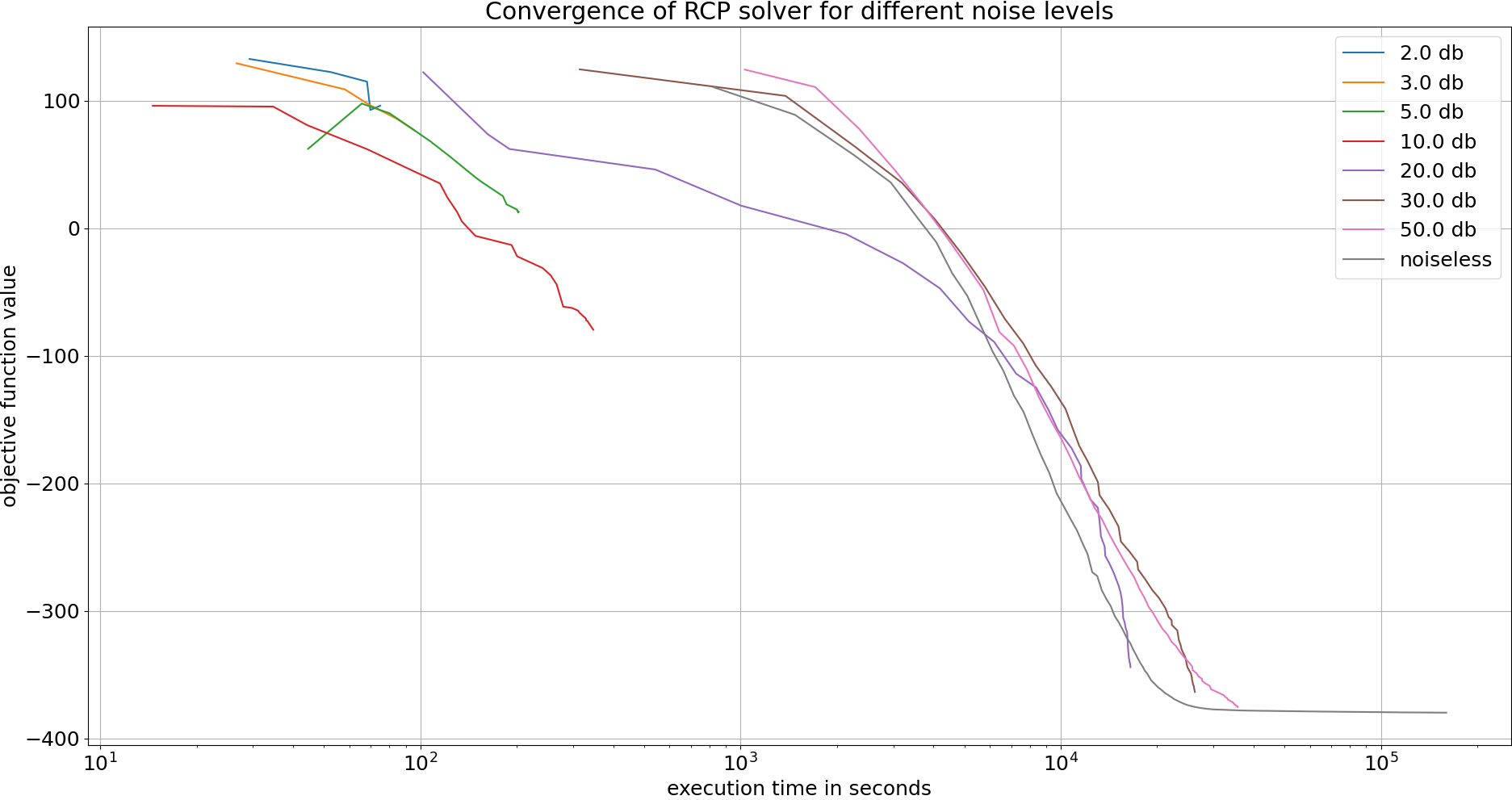
Figure 3: Noise model 2 applied with different signal to noise ratios (SNR) to the problem qap6. The curves demonstrate evolution of objective function value in time. Noisy simulations are terminated before reaching the optimum value.

Experimental setup

We have been using SDPLib, the standard benchmark in SDP. Not all the instances were suitable for the RCP-based solver, which is slow, comparing to classical ones. Out of the full list of 80+ instances, we picked up a few “good” ones, according to the following simple criteria:

• primal problems only.

• those solved successfully by SCS solver with final objective function close to the reference one (provided by SDPLib).

• small enough, so as to be fast to solve: namely, those which SCS solver managed to solve in less than $200$ seconds.

The list of “good” instances appears in the left-most column of the table of results. Note that not every “good” instance was actually solved by RCP method because of the size. One can hence notice that the final value of the objective function is sometimes substantially different from the reference one, although the timeout parameter was $86400$ seconds. Table 6 lists all the results obtained for 1 day timeout ($86400$ seconds). Namely, we interrupt the execution and return solution reached so far as soon as the timeout has been exceeded but simulation is still running. On some instances, the RCP method converged close to the reference value. Table 7 lists all similar results obtained for 7 day timeout ($604800$ seconds). A few instances did not make any substantial progress beyond the very first iteration of the hit&run algorithm because of their large size, such as theta6, where initial and final objective function values are the same.

One possibility we have not explored yet, would be to employ sparse matrices for very large problems.

All numerical experiments have been conducted on a server equipped with 44 cores / 88 hardware threads of Intel(R) Xeon(R) CPU E5-2699 v4 @ 2.20GHz, hundreds of gigabytes of memory, using RedHat 7 OS and Anaconda environment with Python 3.9 and Numpy, Scipy, CVXPY packages installed. The entire code was written in Python.

During our experimentation, we noticed that enabling multi-threading actually significantly slows down the RCP solver. We attribute this behaviour to some software issues, which we did not investigate in depth. Instead, we run all the instances in a separate process without multi-threading, utilising a single CPU core per problem.

Implementation details

In practice, we faced certain challenges trying to implement RCP as presented. A few modifications in the main algorithms have been made to address those issues:

1. In the current implementation, the boundary points are computed by the classical generalised eigensolver from Scipy package, which expects a positive definite matrix $B$ (as in Lemma 5), where the problem $Av_{i}=-\lambda_{i}Bv_{i}$ is considered. The (imperfect) quantum eigensolver is modelled by adding an artificial noise to the eigenvalues. In our case, the matrix $A$ is negative (semi)definite, while $B$ is sign indefinite. We actually solve the problem $\mu_{i}(-A)v_{i}=Bv_{i}$ and then take the reciprocal $\lambda_{i}=1/\mu_{i}$. Moreover, when $A$ is close to semi-definiteness, the eigensolver becomes unstable. If that case, we add a tiny value to diagonal elements of $A$ in order to make it strictly positive definite and repeat the eigensolve one more time.

2. In Section C, the pseudocode of Algorithm H&R_SDP in Line 5 performs the isotropization via computation of a square root of matrix $Y$. The same result can be obtained faster via Cholesky decomposition, which is actually done in our code.

3. In Line 7 of the same algorithm (H&R_SDP), a point $y^{(i+1)}$ is generated inside the segment $[\underline{x},\bar{x}]$. In our implementation, we prevent the point from taking end values by a small margin (about $0.001$ of the segment size).

4. In Lines 8 to 10 of the same algorithm (H&R_SDP), the loop is repeated a number of times (by default up to $200$ attempts before we claim no further improvements can be done). Instead of generating a new couple of boundary points $\underline{x}$, $\bar{x}$ in every iteration of the inner loop, which is very expensive, we repeat Line 7 five times. If $y^{(i+1)}$ remains infeasible, Line 6 is activated.

5. In the same algorithm (H&R_SDP), on Line 3 instead of using the same starting point $x^{(0)}$, we use the last feasible $y$ obtained after previous invocation of H&R_SDP algorithm.

6. The mixing time $M$ is equal to 10 in all simulations. The number $N$ of samples generated in every outer iteration is equal to the number of variables multiplied by $100$. The latter factor is accountable for the slow performance on large problem instances, although the big number of samples provides better convergence rate.

Sometimes, a slightly deeper minimum can be attained without steps (c) to (e), but this depends on randomisation. For the hard instances, these steps bring a noticeable improvement of convergence.

Observations

For the qap6 instance, the time spent by the different modules is distributed as follows (as percentage of the total execution time):

Computation of $F(x)=F_{0}+\sum_{i=1}^{n}x_{i}F_{i}$:	$41\,\%$
Computation of generalised eigen-values:	$22.3\,\%$
Cholesky decomposition:	$6\,\%$
Generation of random vectors:	$5.2\,\%$
Other subroutines:	$25.5\,\%$

Cholesky decomposition is used to check feasibility of the constraint $F(x)\preceq 0$ and for isotropization. Surprisingly, the computation of $F(x)$ dominates the total run time, although it is implemented very rationally (one line of Python code) with full utilisation of Numpy optimised backend.

Volume shrinkage

It might be insightful to see how the volume of convex body is shrinking as iteration process progresses. Again, we selected the qap6 instance for demonstration purposes. This particular instances is challenging (sensitive to sampling scheme), but large enough and solvable in a reasonable time. Fig. 4 shows minimum, maximum and mean eigenvalues of the covariance matrix of a cloud of points sampled on every iteration of hit&run algorithm.

Figure 4: Here we demonstrate the process of shrinking of convex body volume over iterations. The volume is roughly proportional to determinant of the covariance matrix of a cloud of sampled points. Since determinant of high-dimensional covariance matrix is either very big or very small, a better visual experience can be drawn from the behaviour of extreme eigen-values as well as the mean one. The data were obtained for qap6 problem.

Appendix E Results of the Implementation

Table 6: An overview of the behaviour of RCP on a subset of smaller problems from SDPLIB, a well-known benchmark, within a 24-hour time limit ($86400$ seconds): Instance name, dimensions (first is the number of constraint matrices), reference objective function value, objective function value at termination of RCP, initial objective function at the beginning of RCP, DIMACS Error 1 Borchers (1999); Mittelmann (2003) at termination, DIMACS Error 2 Borchers (1999); Mittelmann (2003) at termination, and run-time in seconds.

Instance	size	Ref.	RCP(T)	Initial	Err1(T)	Err2(T)	Time [s]
gpp100	101x100x100	-44.94	-44.94	-18.40	950.45	0.0	86400.32
gpp124-1	125x124x124	-7.34	-6.34	18.08	152.92	0.0	86400.30
gpp124-2	125x124x124	-46.86	-45.77	-19.86	718.02	0.0	86400.34
gpp124-3	125x124x124	-153.01	-150.81	-97.13	815.00	0.0	86400.26
gpp124-4	125x124x124	-418.99	-407.43	-267.03	1551.43	0.0	86400.36
hinf1	13x14x14	2.03	2.09	2.25	7.30	0.0	84.31
hinf10	21x18x18	108.71	122.41	151.07	4998.56	0.0	294.37
mcp100	100x100x100	226.16	226.27	318.12	0.11	0.0	86400.23
mcp124-1	124x124x124	141.99	160.95	250.15	0.08	0.0	86400.27
mcp124-2	124x124x124	269.88	282.22	383.00	0.11	0.0	86400.25
mcp124-3	124x124x124	467.75	486.34	614.28	0.15	0.0	86400.25
mcp124-4	124x124x124	864.41	901.95	1120.64	0.23	0.0	86400.24
mcp250-2	250x250x250	531.93	741.00	758.01	0.12	0.0	86400.73
mcp250-3	250x250x250	981.17	1238.95	1272.45	0.17	0.0	86400.63
mcp250-4	250x250x250	1681.96	2100.18	2155.74	0.26	0.0	86400.76
qap5	136x26x26	-436.00	-435.98	256.19	82.88	0.0	12641.77
qap6	229x37x37	-381.44	-379.29	187.39	20.77	0.0	86400.19
qap7	358x50x50	-424.82	-178.42	290.45	10.08	0.0	86400.27
qap8	529x65x65	-756.96	-12.57	420.27	8.71	0.0	86400.32
qap9	748x82x82	-1409.94	-38.38	745.86	10.78	0.0	86400.40
theta1	104x50x50	23.00	23.00	53.33	106.62	0.0	5967.03
theta2	498x100x100	32.88	145.51	152.09	826.16	0.0	86400.38
theta3	1106x150x150	42.17	82.34	82.34	568.98	0.0	86401.44
theta4	1949x200x200	50.32	147.05	147.05	1186.88	0.0	86403.63
theta5	3028x250x250	57.23	255.70	255.70	2327.25	0.0	86407.97
theta6	4375x300x300	63.48	410.29	410.29	4106.66	0.0	86420.12
truss1	6x13x13	-9.00	-9.00	-7.10	5.90	0.0	17.30
truss2	58x133x133	-123.38	-123.00	-21.46	75.54	0.0	86400.21
truss3	27x31x31	-9.11	-9.11	-5.23	4.78	0.0	794.89
truss4	12x19x19	-9.01	-9.00	-5.83	5.38	0.0	89.30

Table 7: An overview of the behaviour of RCP on a subset of smaller problems from SDPLIB, a well-known benchmark, within a week long time limit ($604800$ seconds): Instance name, dimensions (first is the number of constraint matrices), reference objective function value, objective function value at termination of RCP, initial objective function at the beginning of RCP, DIMACS Error 1 Borchers (1999); Mittelmann (2003) at termination, DIMACS Error 2 Borchers (1999); Mittelmann (2003) at termination, and run-time in seconds.

Instance	size	Ref.	RCP(T)	Initial	Err1(T)	Err2(T)	Time [s]
gpp100	101x100x100	-44.94	-44.94	-18.40	950.46	0.0	82692.28
gpp124-1	125x124x124	-7.34	-7.34	18.08	212.81	0.0	205997.33
gpp124-2	125x124x124	-46.86	-46.86	-19.86	872.42	0.0	149677.75
gpp124-3	125x124x124	-153.01	-153.01	-97.13	862.31	0.0	153632.17
gpp124-4	125x124x124	-418.99	-418.99	-267.03	1667.97	0.0	164294.46
hinf1	13x14x14	2.03	2.09	2.25	7.30	0.0	60.85
hinf10	21x18x18	108.71	122.41	151.07	4998.56	0.0	240.51
mcp100	100x100x100	226.16	226.16	318.12	0.11	0.0	74340.28
mcp124-1	124x124x124	141.99	141.99	250.15	0.07	0.0	188645.49
mcp124-2	124x124x124	269.88	269.88	383.00	0.10	0.0	178055.59
mcp124-3	124x124x124	467.75	467.75	614.28	0.14	0.0	171032.22
mcp124-4	124x124x124	864.41	864.41	1120.64	0.20	0.0	168804.84
mcp250-2	250x250x250	531.93	579.59	758.01	0.08	0.0	604800.46
mcp250-3	250x250x250	981.17	1036.79	1272.45	0.12	0.0	604800.48
mcp250-4	250x250x250	1681.96	1775.46	2155.74	0.17	0.0	604800.49
qap5	136x26x26	-436.00	-435.98	256.19	82.88	0.0	11396.36
qap6	229x37x37	-381.44	-379.67	187.39	20.75	0.0	127062.87
qap7	358x50x50	-424.82	-423.03	290.45	11.47	0.0	410249.13
qap8	529x65x65	-756.96	-744.99	420.27	10.04	0.0	604800.31
qap9	748x82x82	-1409.94	-965.46	745.86	11.90	0.0	604800.37
theta1	104x50x50	23.00	23.00	53.33	106.62	0.0	5088.24
theta2	498x100x100	32.88	50.36	152.09	287.07	0.0	604800.34
theta3	1106x150x150	42.17	76.34	82.34	531.18	0.0	604800.62
theta4	1949x200x200	50.32	143.99	147.05	1188.87	0.0	604802.40
theta5	3028x250x250	57.23	255.70	255.70	2327.25	0.0	604805.45
theta6	4375x300x300	63.48	410.29	410.29	4106.66	0.0	604811.28
truss1	6x13x13	-9.00	-9.00	-7.10	5.90	0.0	16.35
truss2	58x133x133	-123.38	-123.00	-21.46	75.54	0.0	57755.23
truss3	27x31x31	-9.11	-9.11	-5.23	4.78	0.0	684.62
truss4	12x19x19	-9.01	-9.00	-5.83	5.38	0.0	81.22

References

- Boyd and Vandenberghe (2004) Stephen P Boyd and Lieven Vandenberghe, Convex optimization (Cambridge university press, 2004).
-
Note (1)
Indeed, if is convex,
by introducing a slack variable , we obtain an equivalent optimization problem of the form (1)
. - Anjos and Lasserre (2011) Miguel F Anjos and Jean B. Lasserre, Handbook on semidefinite, conic and polynomial optimization, Vol. 166 (Springer Science & Business Media, 2011).
- Note (2) We still assume there are two Euclidean balls and inscribed and outscribed to the feasible set of SDP, which is known as the spectrahedron. Radius of the ball above can also be seen as an upper bound on the trace of an optimal primal solution of an SDP. Notice that in the case of a general SDP, parameters and are not constants independent of dimension, but do grow with the dimension.
- Majumdar et al. (2020) Anirudha Majumdar, Georgina Hall, and Amir Ali Ahmadi, “Recent scalability improvements for semidefinite programming with applications in machine learning, control, and robotics,” Annual Review of Control, Robotics, and Autonomous Systems 3, 331–360 (2020).
- Khot et al. (2007) Subhash Khot, Guy Kindler, Elchanan Mossel, and Ryan O’Donnell, “Optimal inapproximability results for MAX-CUT and other 2-variable CSPs?” SIAM Journal on Computing 37, 319–357 (2007).
- Khot (2010) S. Khot, “On the unique games conjecture (invited survey),” in 2012 IEEE 27th Conference on Computational Complexity (IEEE Computer Society, Los Alamitos, CA, USA, 2010) pp. 99–121.
- Khot and Vishnoi (2015) Subhash A Khot and Nisheeth K Vishnoi, “The unique games conjecture, integrality gap for cut problems and embeddability of negative-type metrics into l1,” Journal of the ACM (JACM) 62, 1–39 (2015).
- Raghavan and Tompson (1987) Prabhakar Raghavan and Clark D. Tompson, “Randomized rounding: A technique for provably good algorithms and algorithmic proofs,” Combinatorica 7, 365–374 (1987).
- Jiang et al. (2020a) Haotian Jiang, Tarun Kathuria, Yin Tat Lee, Swati Padmanabhan, and Zhao Song, “A faster interior point method for semidefinite programming,” in 2020 IEEE 61st Annual Symposium on Foundations of Computer Science (FOCS) (IEEE, 2020) pp. 910–918.
- Mosek (2020) APS Mosek, “The mosek optimization software,” (2020), online at http://www.mosek.com.
- Blum et al. (2012) Lenore Blum, Felipe Cucker, Michael Shub, and Steve Smale, Complexity and real computation (Springer Science & Business Media, 2012).
- Yurtsever et al. (2019) Alp Yurtsever, Joel A Tropp, Olivier Fercoq, Madeleine Udell, and Volkan Cevher, “Scalable semidefinite programming,” arXiv:1912.02949 (2019).
- Ganzhorn et al. (2019) Marc Ganzhorn, Daniel J. Egger, Panagiotis Kl. Barkoutsos, Pauline Ollitrault, Gian Salis, Nikolaj Moll, Andreas Fuhrer, Peter Mueller, Stefan Woerner, Ivano Tavernelli, and Stefan Filipp, “Gate-efficient simulation of molecular eigenstates on a quantum computer,” Phys. Rev. Applied 11, 044092 (2019).
- Havlicek et al. (2019) Vojtech Havlicek, Antonio D. Corcoles, Kristan Temme, Aram W. Harrow, Abhinav Kandala, Jerry M. Chow, and Jay M. Gambetta, “Supervised learning with quantum-enhanced feature spaces,” Nature 567, 209 – 212 (2019).
- Egger et al. (2020) Daniel J Egger, Claudio Gambella, Jakub Marecek, Scott McFaddin, Martin Mevissen, Rudy Raymond, Andrea Simonetto, Stefan Woerner, and Elena Yndurain, “Quantum computing for finance: state of the art and future prospects,” IEEE Transactions on Quantum Engineering (2020).
- Garg et al. (2021) Ankit Garg, Robin Kothari, Praneeth Netrapalli, and Suhail Sherif, “No Quantum Speedup over Gradient Descent for Non-Smooth Convex Optimization,” in 12th Innovations in Theoretical Computer Science Conference (ITCS 2021), Leibniz International Proceedings in Informatics (LIPIcs), Vol. 185, edited by James R. Lee (Schloss Dagstuhl–Leibniz-Zentrum für Informatik, Dagstuhl, Germany, 2021) pp. 53:1–53:20.
- Brandao and Svore (2017) F. G. S. L. Brandao and K. M. Svore, “Quantum speed-ups for solving semidefinite programs,” in 2017 IEEE 58th Annual Symposium on Foundations of Computer Science (FOCS) (2017) pp. 415–426.