AnoSeg: Anomaly Segmentation Network Using Self-Supervised Learning

Abstract

Anomaly segmentation, which localizes defective areas, is an important component in large-scale industrial manufacturing. However, most recent researches have focused on anomaly detection. This paper proposes a novel anomaly segmentation network (AnoSeg) that can directly generate an accurate anomaly map using self-supervised learning. For highly accurate anomaly segmentation, the proposed AnoSeg considers three novel techniques: Anomaly data generation based on hard augmentation, self-supervised learning with pixel-wise and adversarial losses, and coordinate channel concatenation. First, to generate synthetic anomaly images and reference masks for normal data, the proposed method uses hard augmentation to change the normal sample distribution. Then, the proposed AnoSeg is trained in a self-supervised learning manner from the synthetic anomaly data and normal data. Finally, the coordinate channel, which represents the pixel location information, is concatenated to an input of AnoSeg to consider the positional relationship of each pixel in the image. The estimated anomaly map can also be utilized to improve the performance of anomaly detection. Our experiments show that the proposed method outperforms the state-of-the-art anomaly detection and anomaly segmentation methods for the MVTec AD dataset. In addition, we compared the proposed method with the existing methods through the intersection over union (IoU) metric commonly used in segmentation tasks and demonstrated the superiority of our method for anomaly segmentation.

1 Introduction

Anomaly segmentation is the process that localizes anomaly regions. In the real world, since the number of anomaly data is very limited, conventional anomaly segmentation methods are trained using only normal data. Typically, many anomaly segmentation methods are based on anomaly detection techniques because the real dataset includes few anomaly images without the ground truth (GT) mask. Therefore, these methods are not trained directly on pixel-level segmentation and they are difficult to generate anomaly maps similar to GT masks.

Specifically, existing reconstruction-based methods using autoencoder (AE) (An & Cho (2015); Baur et al. (2018); Sakurada & Yairi (2014); Chen et al. (2017); Bergmann et al. (2019)) and generative adversarial network (GAN) (Akcay et al. (2018); Deecke et al. (2018); Schlegl et al. (2017); Zenati et al. (2018)) are trained to learn reconstruction of normal images and determine anomaly if the test sample has the high reconstruction error for an abnormal region. However, reconstruction-based methods often restore even non-complex anomaly regions, which degrade the performance on both anomaly detection and segmentation. Therefore, the anomaly map in Fig. 1(b) greatly differs from the corresponding GT mask. Alternative methods have been recently studied by using the high-level learned representation for anomaly detection and segmentation. These methods use a pretrained model to extract a holistic representation of a given image and compare it to the representation of a normal image. Also, several existing methods use patches, splitting a given image to perform anomaly segmentation. By extracting representations from an image patch, these methods compute the scores of the image patches and combine them to generate the final anomaly map. Therefore, the quality of anomaly maps is highly correlated with the patch size. The uninformed students (US) (Bergmann et al. (2020)) in Figs. 1(c) and (d) are trained using a small patch size (17 x 17) and a large patch size (65 x 65), respectively. Therefore, as shown in Fig. 1(d), US_{65 x 65} is difficult to detect small anomaly regions. Patch SVDD (Yi & Yoon (2020)) and SPADE (Cohen & Hoshen (2020)) use feature maps of multiple scales to detect anomaly regions with various sizes. However, as shown in Figs. 1(e) and (f), these methods approximately detect anomaly regions. In addition, in GradCAM-based methods, GradCAM (Selvaraju et al. (2017)) is used to generate anomaly maps to detect regions that influence the decision of the trained model (Kimura et al. (2020); Venkataramanan et al. (2020)). CutPaste (Li et al. (2021)) introduces a self-supervised framework using a simple effective augmentation that encourages the model to find local irregularities. CutPaste also performs anomaly localization through GradCAM by extending the model to use patch images after training the classifier. However, these methods are not aimed at anomaly segmentation and detect anomaly regions using a modified anomaly detection method. Generally, to improve the segmentation performance, a methodology that can be learned pixel-wise should be considered. Therefore, existing methods cannot clearly detect anomalies because it is difficult that directly use the pixel-wise loss such as a mean squared error typically used in the segmentation task.

To handle this problem, this paper proposes a new methodology that can directly learn the segmentation task. The proposed anomaly segmentation network (AnoSeg) can generate an anomaly map to segment the anomaly region that is unrelated to the normal class. The goal of AnoSeg is to generate an anomaly map that represents the normal class region within a given image for anomaly segmentation, unlike the existing methods to indirectly extract anomaly maps. For this goal, our AnoSeg proposes three following approaches. First, as shown in Fig. 2, AnoSeg uses the segmentation loss directly using the synthesized data generated through hard augmentation, which generates data shifted away from the input data distribution. Second, AnoSeg learns to generate the anomaly map and reconstruct normal images.

Also, an adversarial loss is applied by using a generated anomaly map and an input image. Unlike the existing GAN, the discriminator of AnoSeg determines whether the image is a normal class and whether the anomaly map is focused on the normal region. Since the anomaly map learns the normal sample distribution, AnoSeg has high generalization for unseen normal and anomaly regions even with a small number of normal samples.

Third, we propose the coordinate channel concatenation using a coordinate vector based on coordconv (Liu et al. (2018)). Anomaly regions in a particular category often depend on the location information of a given image. Therefore, the proposed coordinate vector helps to understand the positional relationship of normal and anomaly regions in the input image. As a result, Fig. 1(h) shows that the anomaly map of AnoSeg is very similar to GT even without thresholding. Moreover, we describe how to perform the anomaly detection using the generated anomaly map. By simply extending the model using an anomaly map to the existing GAN-based method (Sabokrou et al. (2018)), we could achieve 96.4 area under ROC curve (AUROC) for image-level localization, which is a significant improvement over conventional state-of-the-art (SOTA) methods. As a result, the proposed method achieves SOTA performance on the MVTec Anomaly Detection (MVTec AD) dataset for anomaly detection and segmentation compared to conventional methods without using a pretrained model. The main contributions of this study are summarized as follows:

Figure 1: Comparison of anomaly maps (before thresholding) of the proposed method with the SOTA methods in the MVTec-AD dataset. Except for the proposed method, anomaly maps of existing methods are normalized to [0, 1].

• We propose a novel anomaly segmentation network (AnoSeg) to directly generate an anomaly map. AnoSeg generates detailed anomaly maps using the holistic approaches to maximize segmentation performance.

• The proposed anomaly map can also be used in existing anomaly detection methods to improve the anomaly detection performance.

• In anomaly segmentation and detection, AnoSeg outperforms SOTA methods on the MVTec AD dataset in terms of intersection over union (IoU) and AUROC. Additional experiments using IoU metric also show that AnoSeg is robust for thresholding.

2 Related Works

Anomaly detection is a research topic that has received considerable attention. Anomaly detection and segmentation are usually performed via unsupervised methods using the generative model for learning the distribution of a certain class. In these methods, GAN (Goodfellow et al. (2014)) or VAE (Kingma & Welling (2014)) learned the distribution of a certain class and used the difference between a reconstructed image and an input for anomaly detection (An & Cho (2015); Chen et al. (2017); Sakurada & Yairi (2014); Sabokrou et al. (2018)). In addition, initial deep learning-based anomaly segmentation methods focused on generative models such as GAN (Schlegl et al. (2017)) and AE (Bergmann et al. (2019)). However, these approaches could have high reconstruction performance for simple anomaly regions. Recently, methods using a representation of an image patch have shown great effectiveness in anomaly detection (Yi & Yoon (2020); Cohen & Hoshen (2020)). In Bergmann et al. (2020), US was trained to mimic a pretrained teacher by dividing an image into patches. In recent studies (Li et al. (2021)), an activation map that visualizes the region of interest through GradCAM (Selvaraju et al. (2017)) was applied to anomaly detection. Kimura et al. (2020) generated an activation map using GradCAM to focus only on the reconstruction loss of the ROI. Venkataramanan et al. (2020) improved the detection performance using an activation map in the training process. Liznerski et al. (2021) apply one-class classification on features extracted from a fully convolutional network and use receptive field upsampling with Gaussian smoothing to extract anomaly map. However, in these existing methods, it is difficult to apply the loss related to anomaly segmentation because the model does not directly generate an anomaly map by using the modified anomaly detection method. Our method is different from the conventional methods which use GradCAM to indirectly extract the activation map. Instead, the proposed method directly extracts and supervises the anomaly map. Therefore, the proposed method discriminates between anomaly and normal regions more accurately compared to previous methods.

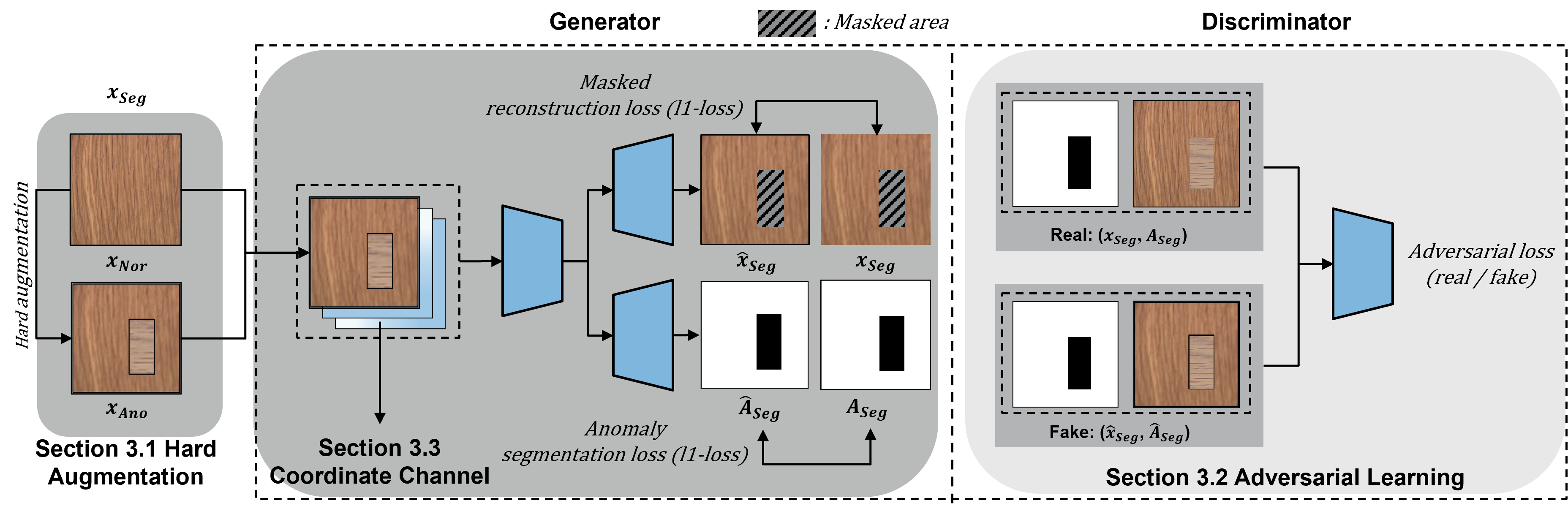
Figure 2: Overview of the training process of the proposed AnoSeg. AnoSeg generates reconstructed images and anomaly maps. To directly generate anomaly maps, AnoSeg applies three novel techniques: hard augmentation, adversarial learning, and coordinate channel concatenation.

3 Proposed Method: AnoSeg

The proposed AnoSeg is a “holistic” approach which incorporates three techniques: self-supervised learning using hard augmentation, adversarial learning, and coordinate channel concatenation. The details are explained in the following sub-sections.

3.1 Self-supervised Learning Using Hard Augmentation

To train anomaly segmentation directly, an image with an anomaly region and its corresponding GT mask corresponding to the image are required. However, it is difficult to obtain these images and GT masks in the real case. Therefore, the proposed method uses hard augmentation (Tack et al. (2020)) and Cutpaste (Li et al. (2021)) to generate synthetic anomaly data and GT masks. Hard augmentation refers to generating samples shifted away from the original sample distribution. As confirmed in Tack et al. (2020), the hard augmented samples can be used as a negative samples. Therefore, as shown in Fig. 3, we use three types of hard augmentation: rotation, perm, and color jitter. Each augmentation is applied with a 50% chance. Then, like Cutpaste (Li et al. (2021)), the augmented data is pasted into a random region of normal data to generate the synthetic anomaly data and corresponding masks for segmentation. Finally, the anomaly segmentation dataset is composed as follows:

$$x_{Seg}=\left\{x_{Nor},x_{Ano}\right\},A_{Seg}=\left\{A_{Nor},A_{Ano}\right\},$$ (1)

where $x_{seg}$ is a set of normal and synthetic anomaly images, in which $x_{Nor}$ and $x_{Ano}$ are normal images and synthetic anomaly images, respectively. $A_{seg}$ is a set of normal and synthetic anomaly masks, in which $A_{Nor}$ and $A_{Ano}$ are normal masks with all inner values set to one and synthetic anomaly masks, respectively.

Using the anomaly segmentation dataset with a pixel-level loss, we can directly train our AnoSeg. The anomaly segmentation loss $L_{Seg}$ is as follows:

$$L_{Seg}=\mathbb{E}\parallel A_{Seg}-\,\widehat{A}_{Seg}\parallel^{1},$$ (2)

where $\widehat{A}_{Seg}$ indicates the generated anomaly map (normal and anomaly classes). The generated anomaly map has the same size as an input image and outputs a value in the range of [0, 1] for each pixel depending on the importance of the pixel of the input image. However, since the synthetic anomaly data are only subset of various anomaly data, it is difficult to generate a real anomaly maps that are unseen in training phase.

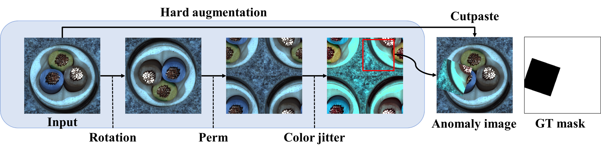
Figure 3: Our synthetic anomaly data augmentation. The synthetic anomaly data is generated by several hard augmentations and Cutpaste (Li et al. (2021)). Synthetic anomaly data is generated by applying a rotation, perm, color jitter, and Cutpaste for each step. Hard augmentations are applied with a 50% chance.

3.2 Adversarial Learning with Reconstruction

To improve the generality for various anomaly data, it is important to train normal region distribution accurately. Therefore, AnoSeg utilizes masked reconstruction loss that uses reconstruction loss only in normal regions to learn only the distribution of normal regions and avoid bias of the distribution of synthetic anomaly regions. Also, since the discriminator inputs a pair for an input image and its GT masks, the discriminator and generator can focus on normal region distribution. Thus, anomaly region cannot be reconstructed well and the detail of the anomaly map can also be improved. Loss functions for adversarial learning are as follows:

$$L_{Adv}=\underset{G}{min}\underset{D}{max}\{\mathbb{E}\;[\log(D(concat(x_{Seg},A_{Seg})))]+\mathbb{E}\;[\log(1-D(concat(\widehat{x}_{Seg},\widehat{A}_{Seg})))]\},$$ (3)

$$L_{Re}=\mathbb{E}\parallel x_{Seg}*A_{Seg}-\,\widehat{x}_{Seg}*A_{Seg}\parallel^{1}/\mathbb{E}\parallel A_{Seg}\parallel^{1},$$ (4)

where $D$, $G$, and $concat$ are a discriminator, a generator, and a concatenation operation, respectively. In Section 5, we demonstrated the effectiveness of adversarial loss.

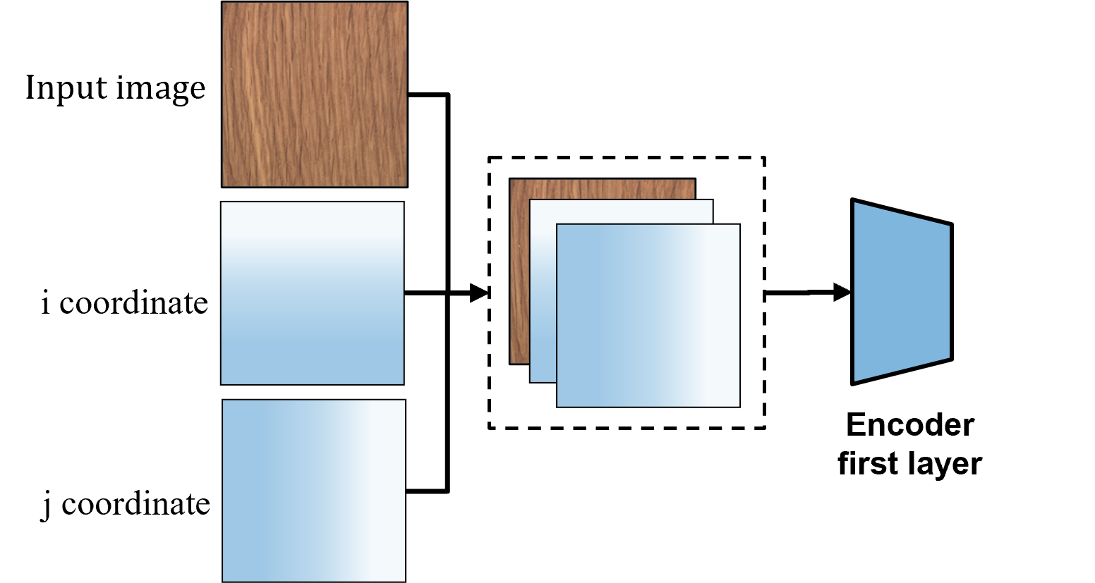
Figure 4: Overall process of the coordinate channel concatenation.

3.3 Coordinate Channel Concatenation

In the typical segmentation task, the location information is the most important information because normal and anomaly regions can be changed depending on where they are located. To provide additional location information, we use a coordinate vector inspired by CoordConv (Liu et al. (2018)). We first generate rank 1 matrices that are normalized to [-1, 1]. Then, we concatenate these matrices with the input image as channels (Fig. 4). As a result, AnoSeg extracts features by considering the positional relationship of the input image. In ablation study, we demonstrated the effectiveness of coordinate channel concatenation.

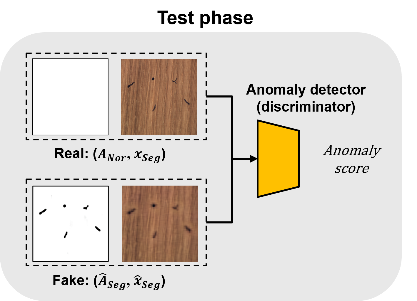
Figure 5: An overview of the proposed anomaly detection method. To obtain anomaly score, the pair of images reconstructed from the anomaly map and the anomaly detector (fake pair) are compared with the pair of the normal mask and the input image (real pair) using a discriminator.

3.4 Anomaly Detection Using Proposed Anomaly Map

In this section, we design a simple anomaly detector that adds the proposed anomaly map to the existing GAN-based detection method (Sabokrou et al. (2018)). The proposed anomaly detector performs anomaly detection by learning only normal data distribution. We simply concatenate the input image and anomaly map to use them as inputs of detector, and apply both an adversarial loss and a reconstruction loss. Then, we use the feature matching loss introduced in (Salimans et al. (2016)) to stabilize the learning of the discriminator and extract the anomaly score. We include a detailed description of the training process for anomaly detection in Appendix A.

In the test process (Fig. 5), the proposed anomaly detector obtains anomaly scores using the discriminator that has learned the normal data distribution. We first assume that the input image is normal, so the mask $A_{Nor}$ with all inner values set to one is used in pairs with the input image. When the input image is really normal, a fake pair (anomaly map and reconstructed image) is similar to the real pair (normal mask and input image), so the anomaly detector has a low anomaly score. On the other hand, when the input image is abnormal, the fake pair is significantly different to the real pair, so it has a high anomaly score. To compare the real and fake pair, the reconstruction loss and the feature matching loss are used as follows:

$$Score=\alpha L_{MSE}(f(concat(x_{Seg},A_{Nor})),f(concat(\widehat{x}_{Seg},\widehat{A}_{Seg})))+\beta L_{MSE}(x_{Seg},\widehat{x}_{Seg}),$$ (5)

where $\alpha$ and $\beta$ are 1 and 0.1, respectively. $A_{Nor}$ and $L_{MSE}$ represent a normal GT mask and the mean squared error, respectively.

Table 1: Performance comparison of anomaly segmentation and detection in terms of pixel-level AUROC and image-level AUROC with the proposed method and conventional SOTA methods on the MVTec AD dataset (Bergmann et al. (2019)). Full results for anomaly detection are added in Table 4 of Appendix A.3.

‘
	Anomaly Segmentation (Pixel-level AUROC)
Method	AEL2	​CAVGA	US	FCDD	Patch SVDD	SPADE	​​Cutpaste	​​Proposed
Bottle	0.86	0.89	0.94	0.97	0.98	0.98	0.98	0.99
Cable	0.86	0.85	0.91	0.90	0.97	0.97	0.90	0.99
Capsule	0.88	0.95	0.92	0.93	0.96	0.99	0.97	0.90
Carpet	0.59	0.88	0.72	0.96	0.93	0.98	0.98	0.99
Grid	0.90	0.95	0.85	0.91	0.96	0.94	0.98	0.99
Hazelnut	0.95	0.96	0.95	0.95	0.98	0.99	0.97	0.99
Leather	0.75	0.94	0.84	0.98	0.97	0.98	0.99	0.98
Metal_nut	0.86	0.85	0.92	0.94	0.98	0.98	0.93	0.99
Pill	0.85	0.94	0.91	0.81	0.95	0.96	0.96	0.94
Screw	0.96	0.85	0.92	0.86	0.96	0.99	0.97	0.91
Tile	0.51	0.80	0.91	0.91	0.91	0.87	0.90	0.98
Toothbrush	0.93	0.91	0.88	0.94	0.98	0.98	0.98	0.96
Transistor	0.86	0.85	0.73	0.88	0.97	0.94	0.93	0.96
Wood	0.73	0.86	0.85	0.88	0.91	0.89	0.96	0.98
Zipper	0.77	0.94	0.91	0.92	0.95	0.97	0.99	0.98
Mean	0.82	0.89	0.88	0.92	0.96	0.96	0.96	0.97
	Anomaly Detection (Image-level AUROC)
Mean	0.71	0.82	0.84	-	0.92	0.86	0.95	0.96
‘

4 Experimental Results

4.1 Evaluation Datasets and Metrics

To verify the anomaly segmentation and detection performance of the proposed method, several evaluations were performed on the MVTec AD dataset (Bergmann et al. (2019)). For the MVTec AD dataset, we resized both training and testing images to the size of 256 × 256, and each training batch contains 16 images. Following the previous works (Bergmann et al. (2019); Venkataramanan et al. (2020); Li et al. (2020)), we adopted the pixel-level and image-level AUROCs to quantitatively evaluate the performance of different methods for anomaly segmentation and detection, respectively. In addition, we used IoU to evaluate anomaly segmentation. For the measurement of IoU, a threshold, which maximizes IoU, was applied in each method.

4.2 Implementation Details

The encoder of AnoSeg consists of the convolution layers of ResNet-18 (He et al. (2016)). The up-sampling layer of decoders consists of one transposed convolution layer and convolution layers. Two decoders of the AnoSeg are composed of five up-sampling layers and two convolution layer to generate an anomaly map and a reconstructed image. The structure of the anomaly detector is the same as the AnoSeg structure except for the decoder that generates the anomaly map. Detailed information on training process and the network architecture is described in Appendix B.

4.3 Experiments on the MVTec AD Dataset

4.3.1 Compared Methods

We compared the reconstruction-based method with the proposed method using autoencoder-L2 ($\text{AE}_{L2}$). GradCAM-based methods (CAVGA (Venkataramanan et al. (2020)) and Cutpaste (Li et al. (2021))) were also compared with the proposed method. Also, we compared the proposed method with the US Bergmann et al. (2020) using the representation of patch images. In our experiment, we compared the US trained with a patch size of $65\times 65$. The proposed method is also compared with FCDD (Liznerski et al. (2021)) using receptive field upsampling. Finally, among the embedding similarity-based methods, the patch SVDD (Yi & Yoon (2020)) and SPADE (Cohen & Hoshen (2020)) were also used for the performance comparison.

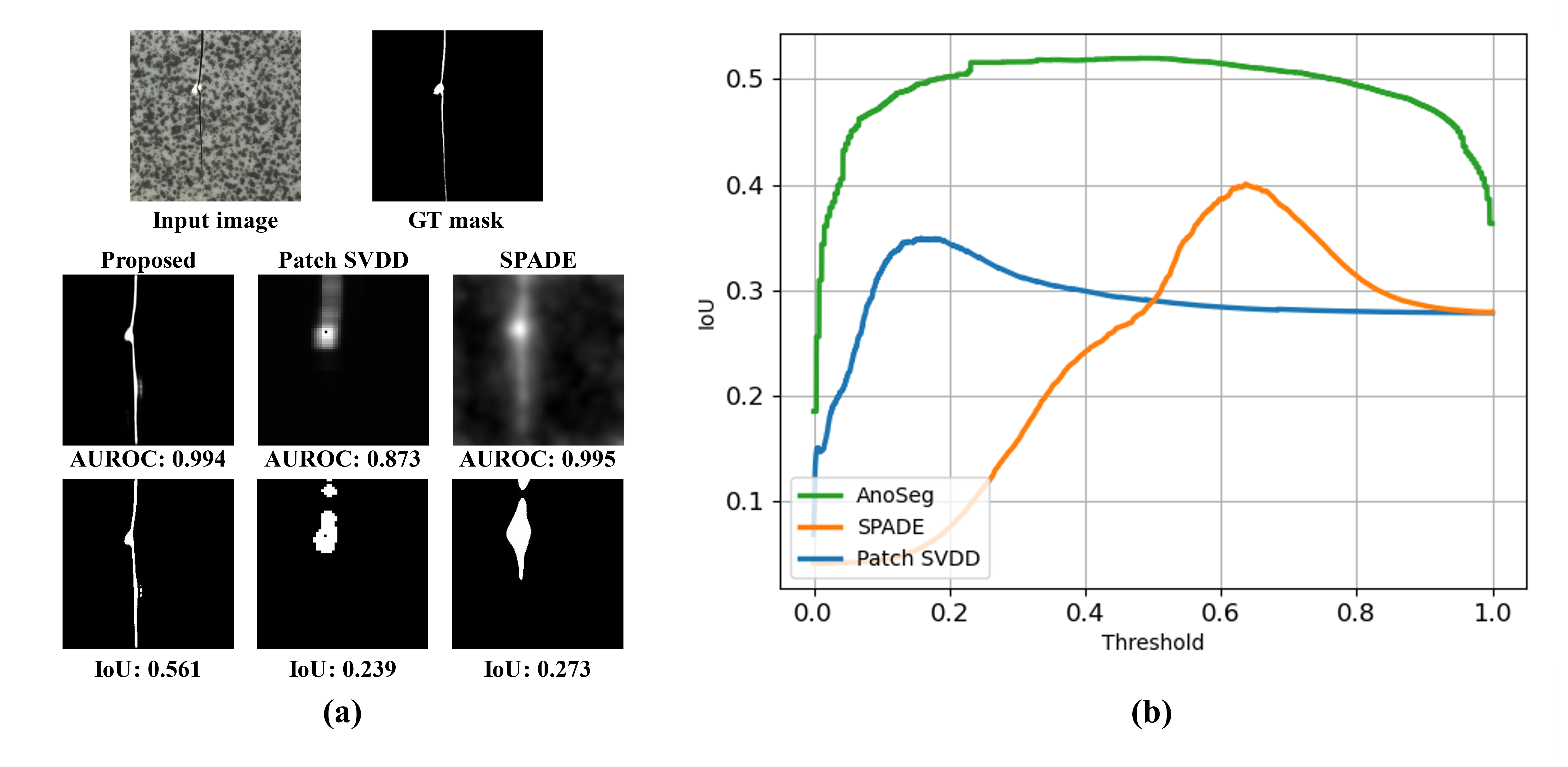
Figure 6: (a) Comparison on AUROC and IoU using Anomaly map and (b) mean IoU change according to the threshold for each category. The x-axis and y-axis represent a threshold and IoU, respectively.

Table 2: Performance comparison of anomaly segmentation in term of mean IoU with the proposed and conventional SOTA methods on the MVTec AD dataset.

‘
	Anomaly Segmentation (IoU)
Method	CAVGA	US	Patch SVDD	SPADE	Proposed
Mean	0.470	0.244	0.427	0.483	0.542
‘

4.3.2 Quantitative Results

We evaluated the anomaly segmentation performance between the proposed method and the existing SOTA methods mentioned in section 4.3.1 using the MVTec AD dataset. As shown in Table 1, the proposed method consistently outperformed all other existing methods evaluated in AUROC. The reconstruction-based methods such as $\text{AE}_{L2}$ used the reconstruction loss as the anomaly score. $\text{AE}_{L2}$ had lower performance (0.82 AUROC) compared to the proposed method. CAVGA (Venkataramanan et al. (2020)) and Cutpaste (Li et al. (2021)) obtained anomaly maps using GradCAM (Selvaraju et al. (2017)), but these anomaly maps highly depend on the classification loss. In addition, compared to the methods using patch image representation such as US, the proposed method achieved higher performance. As a result, AnoSeg outperformed the conventional SOTA, such as Patch SVDD, SPADE, and Cutpaste, by $1\%$ AUROC in anomaly segmentation.

In addition, we evaluated IoU, which is typically used as a metric for segmentation. Table 2 shows the quantitative comparison on IoU. AnoSeg achieved the highest performance compared to other methods in IoU. In particular, Patch SVDD and SPADE achieved 0.96 AUROC similar to AnoSeg in the evaluation of AUROC, but had lower IoU than the proposed method. This is because, unlike the existing method, the proposed method was directly trained for segmentation.

Additionally, we compared the AUROC and IoU metrics for the generated anomaly map in Fig. 6(a). In general, AUROC is affected by the detection performance of the anomaly regions. False positives for normal regions have relatively no impact on AUROC. In the Patch SVDD of Fig. 6(a), there were abnormal regions that cannot be detected. Therefore, the anomaly map of Patch SVDD had lower AUROC compared to other methods. Although the anomaly maps of AnoSeg and SPADE visually show different anomaly maps, the same AUROC was calculated because most anomaly regions are detected in anomaly maps of AnoSeg and SPADE. However, IoU was affected by false positives in normal regions. Therefore, IoU of SPADE had lower performance compared to AUROC. The proposed AnoSeg achieved the highest performance for both IoU and AUROC. These results shows that the proposed method is superior in various aspects of anomaly segmentation.

We compared the anomaly detection performance between the proposed and existing methods using the method introduced in section 4.3.1. As shown in Table 1, the proposed method achieved similar AUROC to existing SOTA methods (Full results are in Appendix A.3). Discriminator of anomaly detector learned representations of images and anomaly maps together. Therefore, with a simple anomaly detection method using the generated anomaly map, we achieve anomaly detection performance similar to that of the existing SOTA.

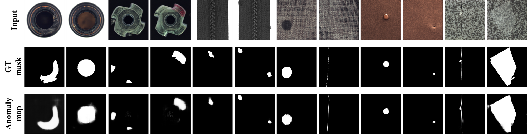
Figure 7: Qualitative results on the MVTec AD dataset for (first row) input image, (second row) GT mask, and (third row) proposed anomaly map.

Table 3: Performance of various configurations on the MVTec AD dataset.

‘
	Ablation study (AUROC / IoU)
Method	Base model (Cutpaste only)	+ Hard augmentation	+ Adversarial learning	+ Coordinate channel
Mean	0.923 / 0.492	0.942 / 0.503	0.951 / 0.527	0.970 / 0.542
‘

4.3.3 Qualitative Results

For the evaluation with existing methods, we visualized anomaly maps of existing and proposed methods in Fig. 1. The output image of $\text{AE}_{L2}$ (Bergmann et al. (2019)) was restored up to the anomaly image region and it was difficult to restore high-frequency regions of the normal image. Also, $\text{US}_{65\times 65}$ could detect large defects, but had poor detection performance for small defects. These results show that patch representations based methods are difficult to accurately localize defects for various sizes. Patch SVDD and SPADE extracted anomaly maps using feature extractions for different sizes to consider defects with various sizes. Therefore, the defects with different sizes could be detected, as shown in Fig. 1. However, these anomaly maps had many false positives for normal regions and approximately detected anomaly regions. In contrast, as shown in Fig. 7, the proposed AnoSeg was trained to generate anomaly maps directly for anomaly segmentation using the segmentation loss. Therefore, the proposed method generated an anomaly map more similar to GT than the results of the existing methods as shown in Fig. 6. More comprehensive results on defect segmentation are given in Appendix C.

4.3.4 Analysis of Threshold Sensitivity

In this section, Patch SVDD and our AnoSeg were compared to verify the performance variation depending on the threshold of the proposed method. IoU was measured by dividing the anomaly score by 10000 units. Fig. 6(b) shows the performance change of AnoSeg, SPADE and Patch SVDD according to a threshold. As shown in Fig. 6(b), the performance of AnoSeg did not significantly change significantly for different thresholds. Therefore, the anomaly map is shown similar to the GT mask even though thresholding was not applied in Fig. 6. On the other hand, Fig. 6(b) shows that Patch SVDD and SPADE had a significant change in performance when the threshold is changed around the threshold with the highest IoU. The result shows that our model is robust against thresholding. By setting the threshold between 0.2 and 0.8, AnoSeg could always achieve better results consistently than other SOTA solutions listed in Table 2.

5 Ablation Study

We modified the generator structure (Section 4.2) to generate the only anomaly map and construct the base model with only Cutpaste applied. Then, we added modules incrementally on the base model, and evaluated with IoU and AUROC scores. The overall results show that the method using all modules improved by 5.4% and 10.2% for AUROC and IoU, respectively, compared to the base model. The effectiveness of each module is described below.

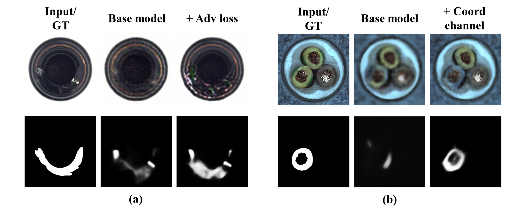
Figure 8: Qualitative results of the ablation study to illustrate the performance of the anomaly segmentation on the MVtec AD dataset.

Hard augmentation  We used images with several hard augmentations applied to train AnoSeg on anomaly regions. Hard augmentations generate samples away from the normal data distribution. Intuitively, synthetic anomaly data applied with hard augmentation can generate more diverse anomaly regions than Cutpaste. Therefore, AnoSeg detected more anomaly regions than the base model. As a result, AUROC and IOU were improved by 2.1% and 1.9% respectively.

Adversarial learning with reconstruction loss  The proposed AnoSeg learns the normal region distribution through adversarial learning. We also use masked reconstruction loss in AnoSeg to apply reconstruction loss only for normal regions to avoid biasing synthetic anomaly regions. As shown in a of Fig. 8(a), the base model is difficult to learn the normal data distribution. Therefore, the reconstructed image of base model partially restores the anomaly regions, and the base model detects anomaly regions as normal regions. In contrast, a model using adversarial learning learns the normal data distribution and can segment between normal and abnormal regions. Therefore, AnoSeg can generate detailed anomaly maps.

Coordinate channel concatenation  To consider the additional location information while performing anomaly segmentation, we concatenated coordinate channels. In Fig. 8(b), the effectiveness of coordinate channel concatenation is confirmed. The yellow cable in the input image changes the class property depending on the location. Therefore, these anomaly regions can be determine as normal if location information is insufficient. Because the base model that does not use the coordinate channel lacks location information, the yellow cable, which is an abnormal area, is reconstructed and determined as a normal area. AnoSeg provides additional location information by connecting the coordinate channel to the input image. As a result, as shown in Fig.8(b) anomaly regions that depend on location information were additionally detected, and AUROC and IOU were improved by 1.9% and 2.8% respectively.

6 Conclusion

This paper presented a novel anomaly segmentation network to directly generate an anomaly map. We proposed AnoSeg, a segmentation model using adversarial learning, and the proposed AnoSeg was directly trained for anomaly segmentation using synthetic anomaly data generated through hard augmentation. In addition, anomaly regions sensitive to positional relationships were more easily detected through coordinate vectors representing the pixel position information. Hence, our approach enabled AnoSeg to be trained to generate anomaly maps with direct supervision. We also applied this anomaly maps to existing methods to improve the performance of anomaly detection. Experimental results on the MVTec AD dataset using AUROC and IoU demonstrated that the proposed method is a specialized network for anomaly segmentation compared to the existing methods.

Appendix A Anomaly Detection Using Proposed Anomaly Map

Here we provide detailed information for the training and loss functions of anomaly detector using the proposed anomaly map from Section 3.4.

A.1 Training Process of Anomaly Detection Method

The proposed anomaly detection method uses an anomaly map generated from the AnoSeg along with the input image to learn the distribution of the normal image and the anomaly map. Therefore, the anomaly detector determines whether the anomaly map is focusing on the normal region of the input image while determining whether the input image is a normal image. Unlike AnoSeg, the proposed anomaly detection method does not use the synthetic anomaly $x_{Ano}$ as a real class in an adversarial loss because discriminator of anomaly detector only needs to learn the normal data distribution for anomaly detection. The loss function for learning the discriminator of the anomaly detector ($L_{Adv}^{AD}$) is as follows:

$$L_{Adv}^{AD}=\underset{G}{min}\underset{D}{max}\{\mathbb{E}\;[\log(1-D(concat(\widehat{x}_{Nor},\widehat{A}_{Nor})))]$$

$$+\mathbb{E}\;[\log(D(concat(x_{Nor},A_{Nor})))]\},$$ (6)

where $\widehat{x}_{Nor}$, $\widehat{A}_{Nor}$, $x_{Nor}$, and $,A_{Nor}$ represent reconstructed a normal image, a anomaly map of AnoSeg, a normal image, and a normal mask, repectively.

Also, to help estimate the normal data distribution, we propose a synthetic anomaly classification loss that discriminates between synthetic data and normal data. As confirmed in (Odena (2016)), the proposed synthetic anomaly classification loss improves the anomaly performance of the discriminator. This synthetic anomaly classification loss is defined as:

$$L_{cls}=\mathbb{E}\;[\log(1-D(concat(x_{Ano},A_{Ano})))]+\mathbb{E}\;[\log(D(concat(x_{Nor},A_{Nor})))].$$

Then, we use the feature matching loss introduced in (Salimans et al. (2016)) to stabilize the learning of the discriminator and extract the anomaly score. The high-level representations of the normal and reconstructed samples are expected to be identical. This loss is given as follows:

$$L_{fea}=\mathbb{E}\parallel f(concat(x_{Nor},A_{Nor}))-\,f(concat(\widehat{x}_{Nor},\widehat{A}_{Nor}))\parallel^{2},$$

where $f(.)$ is the second to the last layer of the discriminator. Fig. 9 shows an overview of the overall training process.

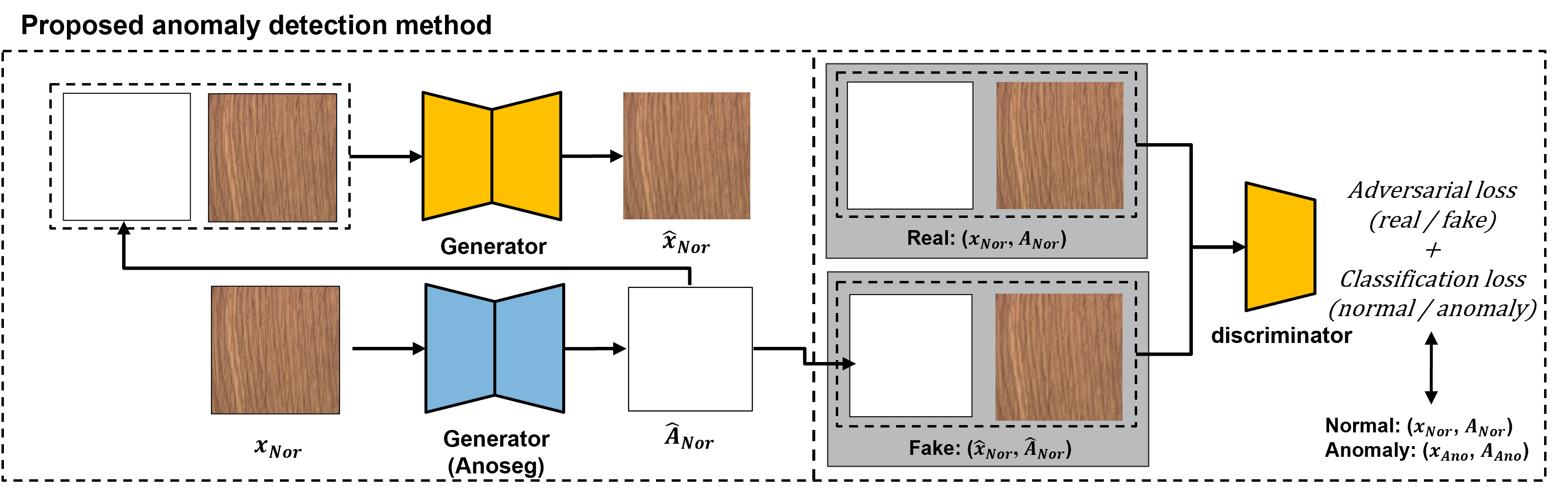
Figure 9: Overview of the training process of the proposed anomaly detection method.

A.2 Quantitative Evaluation of Anomaly Detection in the MVTec AD dataset.

We describe the performance evaluation setting of the existing method that was not included in the main paper due to the length limitation. For performance comparison with existing methods, we used the results from existing literature, excluding the uninformed students method (US) (Bergmann et al. (2020)). US method is only evaluated with PRO scores for anomaly segmentation without the provision of the AUROC for the anomaly segmentation and detection. Therefore, we re-implemented the large patch size (patch size is $65\times 65$) version of the Student method and evaluated it on anomaly detection and segmentation. Tables 4 also shows the class-wise anomaly detection performances for the MVTec AD (AUROC) dataset.

Table 4: Performance comparison of anomaly detection in terms of image-level AUROC with the proposed method and conventional SOTA methods on the MVTec AD dataset (Bergmann et al. (2019)).

‘
	Anomaly Detection (Image-level AUROC)
Method	AEL2	​CAVGA	US	Patch SVDD	SPADE	​​Cutpaste	​​Proposed
bottle	0.80	0.91	0.85	0.99	-	0.98	0.98
Cable	0.56	0.67	0.90	0.90	-	0.81	0.98
Capsule	0.62	0.87	0.82	0.77	-	0.96	0.84
Carpet	0.50	0.78	0.86	0.93	-	0.93	0.96
Grid	0.78	0.78	0.60	0.95	-	0.99	0.99
Hazelnut	0.88	0.87	0.91	0.92	-	0.97	0.98
Leather	0.44	0.75	0.73	0.91	-	1.00	0.99
Metal_nut	0.73	0.71	0.58	0.94	-	0.99	0.95
Pill	0.62	0.91	0.90	0.86	-	0.92	0.87
Screw	0.69	0.78	0.90	0.81	-	0.86	0.97
Tile	0.77	0.72	0.87	0.98	-	0.93	0.98
Toothbrush	0.98	0.97	0.81	1.00	-	0.98	0.99
Transistor	0.71	0.75	0.85	0.92	-	0.96	0.96
Wood	0.74	0.88	0.68	0.92	-	0.99	0.99
Zipper	0.80	0.94	0.90	0.98	-	0.99	0.99
Mean	0.71	0.82	0.84	0.92	0.86	0.95	0.96
‘

A.3 Ablation study of Anomaly Detection Method

We evaluated the effectiveness of the individual components in the proposed anomaly detection method on the MVTec AD dataset, as shown in Table 5. The base model used the same structure as the proposed model, and only the input images were fed except for the mask. The base model compared the features of the input image and the reconstructed image to calculate an anomaly score. However, since the reconstructed image often had anomaly regions restored, the base model has the low performance. The model that the feature matching loss is applied had slightly improved AUROC than the base model. The proposed anomaly detection method performed anomaly detection using input images and anomaly maps. Image-level AUROC was significantly increased by up to 15%. Hence, the model using an anomaly map as an input performed anomaly detection more sensitive than the conventional method using only an input image. Finally, to enhance the estimation of the normal data distribution, we added an anomaly classification loss. This loss helps in estimating the boundaries of the normal data distribution where synthetic anomaly data are separated.

Table 5: Anomaly detection performance of various configurations on the MVTec AD dataset.

‘
	Ablation study (Image-level AUROC)
Method	Base model	+ Feature matching loss	+ Input anomaly map	+ Anomaly classification loss
Mean	0.812	0.842	0.943	0.961
‘

Appendix B Details on the Network Architectures

Table 6 shows the network structure of the proposed method. Each network is described by a list of layers including an output shape, a kernel size, a padding size, and a stride. In addition, batch normalization (BN) and activation function define whether BN is applied and which activation function is applied, respectively. The decoder used for image reconstruction has the same structure as the decoder for generating anomaly map, and AnoSeg uses two decoders. The structure of the proposed anomaly detector also has the same structure as that of AnoSeg. The structure of the AnnoSeg is also available in our code added in the supplementary material. The provided code contains pre-trained weight.

‘
Network	Layer (BN, activation function)	Output size	Kernel	Stride	Pad
Encoder	Resnet-18	8 x 8 x 512	-	-	-
Decoder	Conv 1 (BN, ReLU)	8 x 8 x 512	3 x 3	1	1
	ConvTr 1 (BN, ReLU)	16 x 16 x 512	4 x 4	2	1
	Conv 2 (BN, ReLU)	16 x 16 x 256	3 x 3	1	1
	ConvTr 2 (BN, ReLU)	32 x 32 x 256	4 x 4	2	1
	Conv 3 (BN, ReLU)	32 x 32 x 128	3 x 3	1	1
	ConvTr 3 (BN, ReLU)	64 x 64 x 128	4 x 4	2	1
	Conv 4 (BN, ReLU)	64 x 64 x 128	3 x 3	1	1
	ConvTr 4 (BN, ReLU)	128 x 128 x 128	4 x 4	2	1
	Conv 5 (BN, ReLU)	128 x 128 x 128	3 x 3	1	1
	ConvTr 5 (BN, ReLU)	256 x 256 x 128	4 x 4	2	1
	Conv 6 (BN, ReLU)	256 x 256 x 128	3 x 3	1	1
	Conv 7 (-, Sigmoid)	256 x 256 x 3	3 x 3	1	1
Discriminator	Conv 1 (-, LeakyReLU)	128 x 128 x 64	4 x 4	2	1
	Conv 2 (BN, LeakyReLU)	64 x 64 x 128	4 x 4	2	1
	Conv 3 (BN, LeakyReLU)	32 x 32 x 256	4 x 4	2	1
	Conv 4 (BN, LeakyReLU)	16 x 16 x 512	4 x 4	2	1
	Conv 5 (BN, LeakyReLU)	8 x 8 x 512	4 x 4	2	1
	Conv 6 (BN, LeakyReLU)	4 x 4 x 512	4 x 4	2	1
	Conv 7 (BN, LeakyReLU)	2 x 2 x 128	4 x 4	2	1
	Conv 8 (-, Sigmoid)	1 x 1 x 1	4 x 4	2	1

Table 6: Architectural details of the proposed method. ConvTr denotes a transposed convolution layer and Conv denotes a convolution layer.

Appendix C Analysis of Threshold Sensitivity

In this section, we show the IoU results according to threshold changes for each category in the MVTec AD dataset. As shown in Figs. 10, 11, and 12, compared to SPADE and Patch SVDD, which are comparative methods, the performance difference of the proposed AnoSeg is not large according to the change in the threshold.

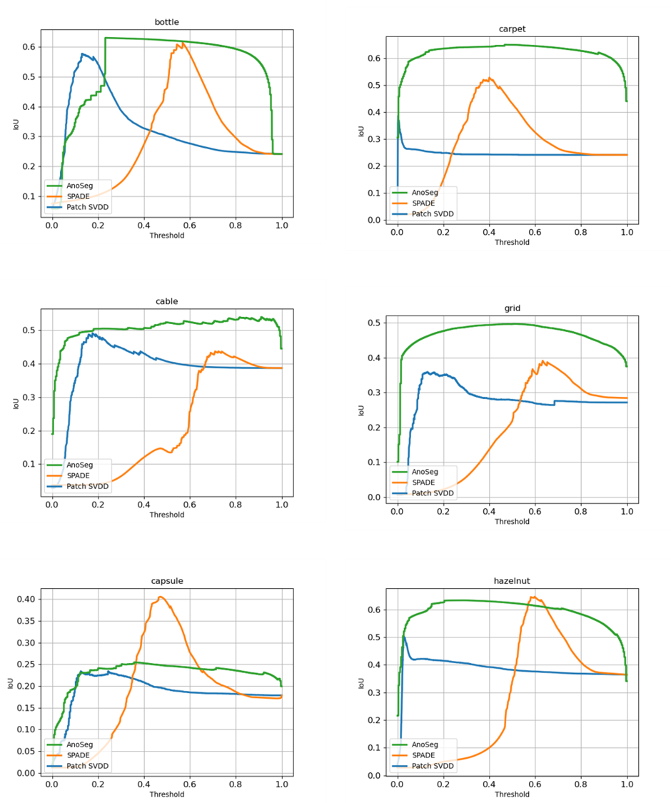
Figure 10: IoU results for each category in the MVTec AD dataset according to the threshold change. (Green: AnoSeg, Orange: SPADE, Blue: Patch SVDD)

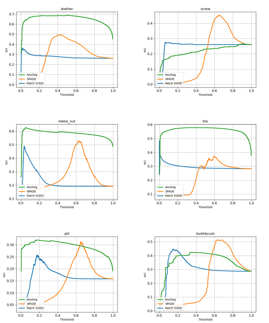
Figure 11: IoU results for each category in the MVTec AD dataset according to the threshold change. (Green: AnoSeg, Orange: SPADE, Blue: Patch SVDD)

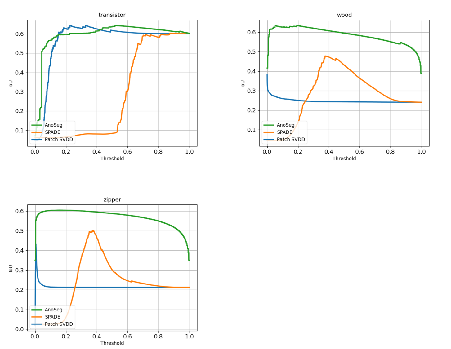
Figure 12: IoU results for each category in the MVTec AD dataset according to the threshold change. (Green: AnoSeg, Orange: SPADE, Blue: Patch SVDD)

Appendix D Qualitative results on the MVTec AD dataset

We provided additional qualitative results of our method on the MVTec AD dataset in Figs. 13, 14, 15, 16, and 17. For each class, an Input image, a proposed anomaly map, and a GT mask are provided. The proposed AnoSeg had the highest performance even for anomaly regions with various sizes.

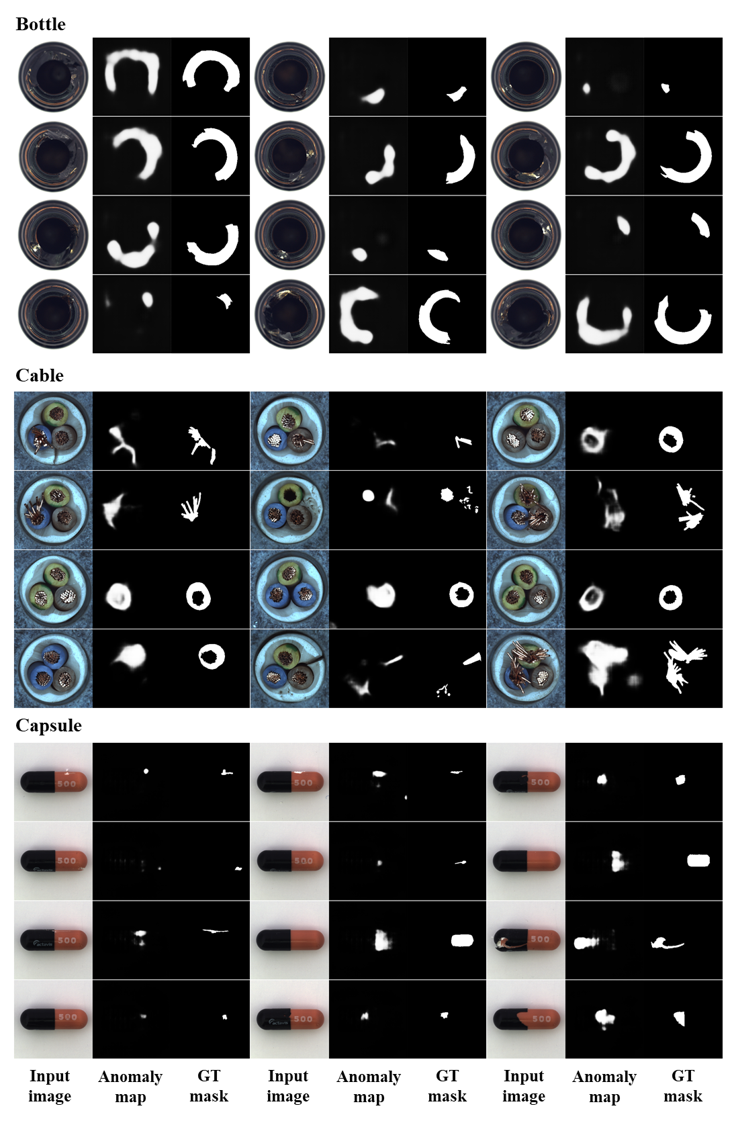
Figure 13: Defect segmentation on MVTec AD dataset. For each sample image, there are an input image, the proposed anomaly map, and its GT mask from left to right.

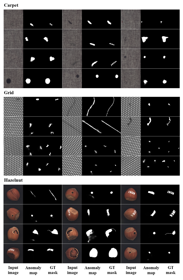
Figure 14: Defect segmentation on MVTec AD dataset. For each sample image, there are an input image, the proposed anomaly map, and its GT mask from left to right.

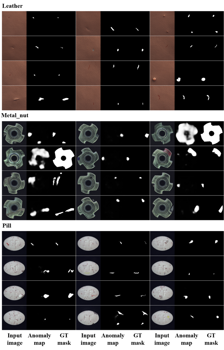
Figure 15: Defect segmentation on MVTec AD dataset. For each sample image, there are an input image, the proposed anomaly map, and its GT mask from left to right.

Figure 16: Defect segmentation on MVTec AD dataset. For each sample image, there are an input image, the proposed anomaly map, and its GT mask from left to right.

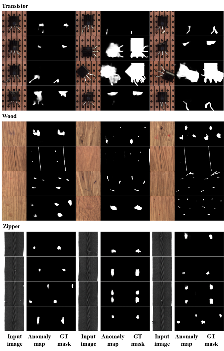
Figure 17: Defect segmentation on MVTec AD dataset. For each sample image, there are an input image, the proposed anomaly map, and its GT mask from left to right.

References

- Akcay et al. (2018) Samet Akcay, Amir Atapour-Abarghouei, and Toby P. Breckon. Ganomaly: Semi-supervised anomaly detection via adversarial training, 2018.
- An & Cho (2015) Jinwon An and Sungzoon Cho. Variational autoencoder based anomaly detection using reconstruction probability. Special Lecture on IE, 2(1):1–18, 2015.
- Baur et al. (2018) Christoph Baur, Benedikt Wiestler, Shadi Albarqouni, and Nassir Navab. Deep autoencoding models for unsupervised anomaly segmentation in brain mr images. In International MICCAI Brainlesion Workshop, pp. 161–169. Springer, 2018.
- Bergmann et al. (2019) P. Bergmann, M. Fauser, D. Sattlegger, and C. Steger. Mvtec ad — a comprehensive real-world dataset for unsupervised anomaly detection. In 2019 IEEE/CVF Conference on Computer Vision and Pattern Recognition (CVPR), pp. 9584–9592, 2019.
- Bergmann et al. (2020) Paul Bergmann, Michael Fauser, David Sattlegger, and Carsten Steger. Uninformed students: Student-teacher anomaly detection with discriminative latent embeddings. In Proceedings of the IEEE/CVF Conference on Computer Vision and Pattern Recognition, pp. 4183–4192, 2020.
- Chen et al. (2017) Jinghui Chen, Saket Sathe, Charu Aggarwal, and Deepak Turaga. Outlier detection with autoencoder ensembles. In Proceedings of the 2017 SIAM international conference on data mining, pp. 90–98. SIAM, 2017.
- Cohen & Hoshen (2020) Niv Cohen and Yedid Hoshen. Sub-image anomaly detection with deep pyramid correspondences. arXiv preprint arXiv:2005.02357, 2020.
- Deecke et al. (2018) Lucas Deecke, Robert Vandermeulen, Lukas Ruff, Stephan Mandt, and Marius Kloft. Image anomaly detection with generative adversarial networks. In Joint european conference on machine learning and knowledge discovery in databases, pp. 3–17. Springer, 2018.
- Goodfellow et al. (2014) Ian Goodfellow, Jean Pouget-Abadie, Mehdi Mirza, Bing Xu, David Warde-Farley, Sherjil Ozair, Aaron Courville, and Yoshua Bengio. Generative adversarial nets. In Advances in neural information processing systems, pp. 2672–2680, 2014.
- He et al. (2016) Kaiming He, Xiangyu Zhang, Shaoqing Ren, and Jian Sun. Deep residual learning for image recognition. In Proceedings of the IEEE conference on computer vision and pattern recognition, pp. 770–778, 2016.
- Kimura et al. (2020) Daiki Kimura, Subhajit Chaudhury, Minori Narita, Asim Munawar, and Ryuki Tachibana. Adversarial discriminative attention for robust anomaly detection. In The IEEE Winter Conference on Applications of Computer Vision, pp. 2172–2181, 2020.
- Kingma & Welling (2014) Diederik Kingma and Max Welling. Auto-encoding variational bayes. In International Conference on Learning Representations, 12 2014.
- Li et al. (2021) Chun-Liang Li, Kihyuk Sohn, Jinsung Yoon, and Tomas Pfister. Cutpaste: Self-supervised learning for anomaly detection and localization. In Proceedings of the IEEE/CVF Conference on Computer Vision and Pattern Recognition, pp. 9664–9674, 2021.
- Li et al. (2020) Zhenyu Li, Ning Li, Kaitao Jiang, Zhiheng Ma, Xing Wei, Xiaopeng Hong, and Yihong Gong. Superpixel masking and inpainting for self-supervised anomaly detection. In 31st British Machine Vision Conference 2020, BMVC 2020, Virtual Event, UK, September 7-10, 2020. BMVA Press, 2020. URL https://www.bmvc2020-conference.com/assets/papers/0275.pdf.
- Liu et al. (2018) Rosanne Liu, Joel Lehman, Piero Molino, Felipe Petroski Such, Eric Frank, Alex Sergeev, and Jason Yosinski. An intriguing failing of convolutional neural networks and the coordconv solution. In S. Bengio, H. Wallach, H. Larochelle, K. Grauman, N. Cesa-Bianchi, and R. Garnett (eds.), Advances in Neural Information Processing Systems, volume 31. Curran Associates, Inc., 2018. URL https://proceedings.neurips.cc/paper/2018/file/60106888f8977b71e1f15db7bc9a88d1-Paper.pdf.
- Liznerski et al. (2021) Philipp Liznerski, Lukas Ruff, Robert A. Vandermeulen, Billy Joe Franks, Marius Kloft, and Klaus Robert Muller. Explainable deep one-class classification. In International Conference on Learning Representations, 2021. URL https://openreview.net/forum?id=A5VV3UyIQz.
- Odena (2016) Augustus Odena. Semi-supervised learning with generative adversarial networks. arXiv preprint arXiv:1606.01583, 2016.
- Sabokrou et al. (2018) Mohammad Sabokrou, Mohammad Khalooei, Mahmood Fathy, and Ehsan Adeli. Adversarially learned one-class classifier for novelty detection. In Proceedings of the IEEE Conference on Computer Vision and Pattern Recognition, pp. 3379–3388, 2018.
- Sakurada & Yairi (2014) Mayu Sakurada and Takehisa Yairi. Anomaly detection using autoencoders with nonlinear dimensionality reduction. In Proceedings of the MLSDA 2014 2nd Workshop on Machine Learning for Sensory Data Analysis, pp. 4–11, 2014.
- Salimans et al. (2016) Tim Salimans, Ian Goodfellow, Wojciech Zaremba, Vicki Cheung, Alec Radford, Xi Chen, and Xi Chen. Improved techniques for training gans. In D. Lee, M. Sugiyama, U. Luxburg, I. Guyon, and R. Garnett (eds.), Advances in Neural Information Processing Systems, volume 29. Curran Associates, Inc., 2016. URL https://proceedings.neurips.cc/paper/2016/file/8a3363abe792db2d8761d6403605aeb7-Paper.pdf.
- Schlegl et al. (2017) Thomas Schlegl, Philipp Seeböck, Sebastian M Waldstein, Ursula Schmidt-Erfurth, and Georg Langs. Unsupervised anomaly detection with generative adversarial networks to guide marker discovery. In International conference on information processing in medical imaging, pp. 146–157. Springer, 2017.
- Selvaraju et al. (2017) Ramprasaath R Selvaraju, Michael Cogswell, Abhishek Das, Ramakrishna Vedantam, Devi Parikh, and Dhruv Batra. Grad-cam: Visual explanations from deep networks via gradient-based localization. In Proceedings of the IEEE international conference on computer vision, pp. 618–626, 2017.
- Tack et al. (2020) Jihoon Tack, Sangwoo Mo, Jongheon Jeong, and Jinwoo Shin. Csi: Novelty detection via contrastive learning on distributionally shifted instances. In H. Larochelle, M. Ranzato, R. Hadsell, M. F. Balcan, and H. Lin (eds.), Advances in Neural Information Processing Systems, volume 33, pp. 11839–11852. Curran Associates, Inc., 2020. URL https://proceedings.neurips.cc/paper/2020/file/8965f76632d7672e7d3cf29c87ecaa0c-Paper.pdf.
- Venkataramanan et al. (2020) Shashanka Venkataramanan, Kuan-Chuan Peng, Rajat Vikram Singh, and Abhijit Mahalanobis. Attention guided anomaly localization in images. In Proceedings of the European Conference on Computer Vision (ECCV), September 2020.
- Yi & Yoon (2020) Jihun Yi and Sungroh Yoon. Patch svdd: Patch-level svdd for anomaly detection and segmentation. In Proceedings of the Asian Conference on Computer Vision, 2020.
- Zenati et al. (2018) Houssam Zenati, Chuan Sheng Foo, Bruno Lecouat, Gaurav Manek, and Vijay Ramaseshan Chandrasekhar. Efficient gan-based anomaly detection. arXiv preprint arXiv:1802.06222, 2018.