Multivariate Anomaly Detection based on Prediction Intervals Constructed using Deep Learning

Abstract

It has been shown that deep learning models can under certain circumstances outperform traditional statistical methods at forecasting. Furthermore, various techniques have been developed for quantifying the forecast uncertainty (prediction intervals). In this paper, we utilize prediction intervals constructed with the aid of artificial neural networks to detect anomalies in the multivariate setting. Challenges with existing deep learning-based anomaly detection approaches include $(i)$ large sets of parameters that may be computationally intensive to tune, $(ii)$ returning too many false positives rendering the techniques impractical for use, $(iii)$ requiring labeled datasets for training which are often not prevalent in real life. Our approach overcomes these challenges. We benchmark our approach against the oft-preferred well-established statistical models. We focus on three deep learning architectures, namely, cascaded neural networks, reservoir computing and long short-term memory recurrent neural networks. Our finding is deep learning outperforms (or at the very least is competitive to) the latter.

1 Introduction

Hawkins (1980) defines an outlier as an observation that ”deviates so significantly from other observations as to arouse suspicion that a different mechanism generated it.” Anomalies, also known as outliers, arise for several reasons, such as intentional acts of malice, collapse or failure of various systems, or fraudulent activity. Detecting these anomalies in a timeous manner is essential in various decision-making processes. Anomaly detection is not to be confused with novelty detection, which is focused on identifying new patterns in the data. However, the techniques used for anomaly detection are often used for novelty detection and vice versa. Carreńo et al. (2020) draw a comparison between the two fields and detail recent advances in the methods applicable to each field.

Anomaly detection, when framed as a classification problem, has been modelled using One-Class Support Vector Machines as far back as the works of Schölkopf et al. (1999). Dealing with a highly imbalanced class distribution (where normal observations far exceed anomalous data points), Schölkopf et al. detect novel patterns by looking at the local density distribution of normal data.

Malhotra et al. (2015) use stacked LSTM networks for anomaly detection in time series. They train the network on non-anomalous data and use it as a predictor over several time steps. The resulting prediction errors are modelled as a multivariate Gaussian distribution, which is then used to assess the likelihood of anomalous behaviour. Later, Malhotra et al. (2016) examine anomaly detection for mechanical devices in the presence of exogenous effects. An LSTM-based Encoder-Decoder scheme is employed that learns to reconstruct time-series behaviour under normalcy and after that uses reconstruction error to detect anomalies. Schlegl et al. (2017) employ a deep convolutional generative adversarial network in an unsupervised manner to learn a manifold of normal anatomical variability and apply it to the task of anomaly detection to aid disease detection and treatment monitoring.

More recently, the research has focused on time-series anomalies that manifest over a period of time rather than at single time points. These are known as range-based or collective anomalies. Thi et al. (2018) consider these and use prediction errors from multiple time-steps for detecting collective anomalies.

Others, such as Zhu and Laptev (2017) use Bayesian Neural Networks (BNNs, Mullachery et al. (2018)) and the Monte Carlo (MC) dropout framework to construct prediction intervals, inspired by Gal (2016) as well as Gal and Ghahramani (2016).

Several probability-based methods have also been successfully applied to the detection of anomalies Aggarwal (2013). If said statistical methods have been applied successfully, why then consider deep learning for anomaly detection at all? We provide three reasons. Firstly, the boundary between normal and anomalous behaviour is at times not precisely defined, or it evolves continually, i.e. the distribution of the data changes dynamically as new instances are introduced to the time series. In such instances, statistical algorithms may sub-perform Sivarajah et al. (2017) unless, for instance, they are retrained continuously to mitigate the changes in the data distributions. Secondly, deep learning algorithms have been shown to scale well in other applications Brink et al. (2016), and we hypothesise that this scalability attribute may extend to cases that require large-scale anomaly detection. Finally, in the most recent M4 competition, it is shown that deep learning produces better prediction intervals than statistical methods Makridakis et al. (2020b). This superior prediction interval result is corroborated by the works of Smyl (2020) in the univariate case as well as Mathonsi and van Zyl (2020) in the multivariate setting, for instance. Our hypothesis is that better prediction intervals can be used to build better anomaly detection machinery.

1.1 Related Work

There have been immense advances made in applying deep learning methods in fields such as forecasting Makridakis et al. (2020b, a), but there is a relative scarcity of deep learning approaches for anomaly detection and its sub-disciplines Kwon et al. (2019); Thudumu et al. (2020).

Considering anomaly detection as a supervised learning problem requires a dataset where each data instance is labeled. With the anomaly detection problem phrased as such, there are general steps usually followed in the literature. Although not identical in their methodologies, even the most recent advances are not dissimilar to approaches first adopted by Malhotra et al. (2015), Chauhan and Vig (2015) and Malhotra et al. (2016), for instance. Generally, methodologies incorporate the following steps:

1. use a deep learning algorithm or architecture (e.g. LSTM, encoder-decoder) for generating forecasts, retain the errors as they are used later for anomaly detection;

2. assume the resultant errors follow a Gaussian (or other) distribution;

3. learn a threshold by maximizing either the $F$-score, precision, recall or some combination thereof on the validation set.

There are also some comprehensive reviews, including, for instance, the works of Adewumi and Akinyelu (2016), who survey deep learning-based methods for fraud detection, Kwon et al. (2019) who focus on techniques and applications related to cyber-intrusion detection, and as recent as Thudumu et al. (2020) who focus on the challenge of detecting anomalies in the domain of big data.

All of these reviews, and the research highlighted above, touch on some critical points related to drawbacks. We summarize these drawbacks in Section 1.2 below.

To avoid ambiguity, all the techniques described in this Section shall further be referred to as ”reviewed techniques.”

1.2 Motivation

All the reviewed techniques, as well as their classical statistical counterparts, have similar drawbacks. Classical techniques such as statistical and probabilistic models are typically suitable only for univariate datasets Makridakis et al. (2020b); Smyl (2020). For the more realistic multivariate case, Li et al. (2017) for instance, propose a method for analyzing multivariate datasets by first transforming the high-dimensional data to a uni-dimensional space using Fuzzy C-Means clustering. They then detect anomalies with a Hidden Markov Model. However, Li et al.’s approach does not fully utilize the additional information provided by the data’s correlation.

Another issue with the reviewed techniques is their reliance on datasets that contain the ground truth, where the anomalies have been labeled. These labels are sometimes also referred to as golden labels. There are difficulties associated with gathering this kind of data in real life, such as the cost of labeling or human error in the labeling process. Even once the reviewed models are trained and parameterized on such data, if available, the dynamic nature of most real-life scenarios would mean the tuned review model might not generalize to new types of anomalies unless retraining is performed continuously Sivarajah et al. (2017).

1.3 Contribution

• We introduce a dynamic threshold-setting approach, which learns and adapts the applicable threshold as new information becomes available.

• No golden labels are required for training or detecting the thresholds, and subsequently detecting the anomalies.

• We consolidate two streams of research by testing our assertions on both outlier and step-change anomalies, whereas previous researchers mostly focused on either one of these.

• We critically analyze forecast machinery, construct competitive prediction intervals using computational means where no statistical methodology is readily applicable, then use all of this information to detect anomalies.

2 Datasets

Our datasets come from a diverse array of economic sectors. We use data from various categories ranging from climate to space aviation. The most important aspect when selecting our datasets is ensuring they are distinctly different in terms of size, attributes, and the composition of normal to anomalous ratio of observations. This data sourcing methodology allows us to forecast for varied horizons, and mitigates biases in model performance. All the datasets are also freely available and have been used extensively in research related to ours and other fields.

2.1 Air Quality Dataset.

We use the Beijing air quality dataset (AQD, Chen (2014)) from UCI. It contains measurements of hourly weather and pollution level for five years spanning January 1${}^{\text{st}}$, 2010 to December 31${}^{\text{st}}$, 2014 at the US embassy in Beijing, China. Meteorological data from the Beijing Capital International Airport are also included. The attribute of interest is the level of pollution in the air (pm2.5 concentration), while Table 1 details the complete feature list.

Table 1: Air Quality Data Description.

Attribute	Description
pm2.5	pm2.5 concentration
DEWP	dew point
TEMP	temperature
PRES	pressure
cbwd	combined wind direction
Iws	cumulated wind speed
Is	cumulated hours of snow
Ir	cumulated hours of rain

2.2 Power Consumption Dataset

The second dataset is UCI’s Household Power Consumption (HPC, Hebrail and Berard (2012)), a multivariate time series dataset detailing a single household’s per-minute electricity consumption spanning December 2006 to November 2010.

With the date and time fields collapsed into a unique identifier, the remaining attributes are described in Table 2.

Table 2: Power Consumption Data Description.

Attribute	Description
global_active_power	total active power consumed ($\mathrm{kW}$)
global_reactive_power	total reactive power consumed ($\mathrm{kW}$)
global_intensity	minute-averaged current intensity ($\mathrm{A}$)
sub_metering_1	active energy for kitchen ($\mathrm{W}\text{\,}\mathrm{h}$)
sub_metering_2	active energy for laundry ($\mathrm{W}\text{\,}\mathrm{h}$)
sub_metering_3	active energy for climate control systems ($\mathrm{W}\text{\,}\mathrm{h}$)

A new attribute is created:

$$\text{sub\_metering\_4}=\dfrac{100}{6}\times\text{global\_active\_power}-\sum_{k=1}^{3}\text{sub\_metering\_}k.$$ (1)

It represents the per-minute active energy consumption not already captured by sub_meterings 1, 2 and 3.

2.3 Bike Sharing Dataset

Next, we consider the UCI Bike Sharing Dataset (BSD, Fanaee-T and Gama (2012)). It catalogues for each hour the number of bikes rented by customers of a bike-sharing service in Washington DC for the 2011 and 2012 calendar years. It includes features such as whether a particular day is a national holiday and the weather and seasonal information. Besides the date-time and index attributes that we collapse into a unique identifier, the dataset has 17 attributes in total. We select only a subset for our analysis, as described in Table 3.

Table 3: Bike Sharing Data Description.

Attribute	Description
holiday	boolean whether day is holiday or not
weekday	day of the week
weathersit	1 if clear, few clouds, partly cloudy 2 if cloudy, mist, broken clouds, few clouds 3 if light snow or rain, thunderstorm, scattered clouds 4 if heavy rain, ice pallets, thunderstorm, snow mist, fog
hum	humidity
temp	normalized temperature in degrees Celsius
casual	count of casual users
registered	count of registered users
cnt	count of total rental bikes, sum of casual and registered

2.4 Bearings Dataset

We also use NASA’s Bearings Dataset (BDS, Lee et al. (2007)). It contains sensor readings on multiple bearings that are operated until failure under a constant load causing degradation. These are one second vibration signal snapshots recorded at ten minute intervals per file, where each file contains $20,480$ sensor data points per bearing. It contains golden labels and has been considered extensively by other researchers in their experimentation; see, for example, Prosvirin et al. (2017).

2.5 Webscope Benchmark Dataset

Lastly, we also evaluate our approach using the Yahoo Webscope Benchmark dataset (YWB, Laptev and Amizadeh (2015)), which is considered a good data source in the research community by, for instance, Thill et al. (2017). It comprises large datasets with golden labels. It is helpful for our purposes as it contains anomalies based on outliers and change-points. The first benchmark, A1, is real site traffic to Yahoo and its related products. The other three, A2, A3, and A4, are synthetic. They all contain three months worth of data-points though of varying lengths, capture frequencies, seasonality patterns and the total number of labeled anomalies.

Because we synthesize anomalies for AQD, BSD and HPC, we only use A1 from YWB. Using the other synthetic benchmarks in YWB may not add further insights to our analysis.

3 Methodology

Our approach utilizes three fundamental steps. We:

1. forecast using deep learning and probability-based models,

2. derive prediction intervals using computational means and built-in density distributions, respectively, and

3. use said prediction intervals to detect anomalies.

Each of the fundamental steps, and intermediate ones, are outlined below.

3.1 Forecasting

3.1.1 AQD

We frame a supervised learning problem where, given the weather conditions and pollution measurements for the current and $23$ prior hours, $t,t-1,t-2,\ldots,t-23$, we forecast the pollution at the next hour $t+1$.

3.1.2 HPC

Given power consumption for 4 weeks, we forecast it for the week ahead. The observations are converted from per-minute to daily aggregates, as illustrated in Figure 1. Seven values comprise a single forecast, one value for each day in the standard week (beginning on a Sunday and ending Saturday). We evaluate each forecast in this aggregated setting as well as with each time step separately.

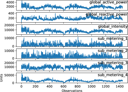
Figure 1: Separate Attribute Plots of the Power Consumption Data Spanning Four Years.

There are only 205 samples available for training, and this may pose a problem for parameters-tuning. So we disregard the standard week, and use the prior $28$ days to forecast the coming $7$ days. This flattening and use of overlapping windows effectively transforms the $205$ samples into a total of $1,418$.

In contrast, the testing framework remains unchanged, i.e. we use the prior four standard weeks to forecast the daily power consumption for the subsequent standard week.

3.1.3 BSD

Given all available information for BSD for the past 3 months, we forecast the total rental bikes for the coming week.

3.1.4 BDS

Given the sensor readings for the past 10 hours, we forecast the readings for the next hour. The mechanical degradation in the bearings occurs gradually over time, so we conduct our analysis using only data points occurring every 10 minutes instead of per-second observations. In total, we have $20,480$ observations across each of the four bearings.

To easily detect the point where the bearing vibration readings begin oscillating dramatically, we transform the signal from the time- to the frequency domain using a Fourier transform.

As depicted in Figure 2, there is an increase in the frequency amplitude for readings progressing to the complete degradation and subsequent failure of each bearing.

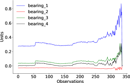
Figure 2: Bearing Sensor Test Frequency Data.

3.1.5 YWB

Lastly, for the YWB, we utilize the last five days worth of observations to forecast traffic to the Yahoo entities for the next hour.

Note, all the above forecast problems can be reframed using different window sizes. We state our chosen window sizes here for reproducibility. These windows were chosen using empirical studies with optimizing based on training accuracy.

For each dataset, we use the relevant forecast framework as described above and subsequently construct prediction intervals with all three deep learning algorithms and all three statistical algorithms.

To a great extent, the treatment of each dataset is not dissimilar. As such, the narrative that follows might overlap. For ease of exposition, all methods are the same unless explicitly stated.

3.2 Preprocessing

We undertake the following steps in preparing the time series data for forecasting. Here we only highlight the most used techniques for all the datasets. NA values are removed. NA is distinct from missing (blank) values, the latter amounting to $4.664\%$ for AQD and $1.252\%$ for HPC, for instance, are imputed using the iterative imputer from the Scikit-learn module Pedregosa et al. (2011), which models each feature with missing values as a function of other features in a round-robin fashion. We set the imputer to parameterize only on past values for each iteration, thus avoiding information leakage from the future testing set.

We label encode categorical values. Label encoding is chosen over one-hot encoding for instances where there are many categories in total (more than five), as the former reduces memory consumption. Furthermore, we normalize the datasets.

All the datasets are composed of time series with different seasonality patterns. In such instances, ANNs tend to struggle with seasonality (Claveria et al., 2015; Smyl, 2020). A standard remedy is to deseasonalize the series first and remove the trend using a statistical procedure like the Seasonal and Trend decomposition using Loess (STL, Cleveland et al. (1990)). For a more detailed treatment of the pre-processing stage, see Mathonsi and van Zyl (2020).

3.3 Algorithms

For benchmarking, the statistical methods used are Multiple Linear Regression (MLR, Matthews (2005)), Vector Autoregression Moving-Average with Exogenous Regressors (VARMAX, Hannan and Deistler (1992)) and Seasonal Autoregressive Integrated Moving-Average with Exogenous Regressors (SARIMAX, Arunraj et al. (2016)).

The deep learning architectures used are the Cascaded Neural Networks based on cascade-correlation (CCN), first published by Fahlman and Lebiere (1990), a variant of the Recurrent Neural Network (RNN, Williams and Zipser (1989)) known as long short-term memory (LSTM, Hochreiter and Schmidhuber (1997)), and one class of reservoir computing, Echo State Networks (ESN, Jaeger (2001)).

For aiding in the construction of prediction intervals, we employ Monte Carlo Dropout Gal and Ghahramani (2016) and the quantile bootstrap Davison and Hinkley (2013) also known as the reverse percentile bootstrap Hesterberg (2014). Details on implementation follow in Section 3.7 and 3.8 respectively.

3.4 Measures of Accuracy

For the point forecasts we use the Root Mean Squared Error (RMSE) that gives error in the same units as the forecast variable itself.

RMSE $$=\sqrt{\dfrac{1}{n}\sum_{t=1}^{n}\left(y_{t}-\hat{y}_{t}\right)^{2}},$$ (2)

where there are $n$ forecasts, $y_{t}$ is the out-of-sample observation and $\hat{y}_{t}$ the forecast at time $t$.

For the prediction intervals we use the Mean Interval Score (MIS, Gneiting and Raftery (2007)), averaged over all out-of-sample observations.

$$\text{MIS${}_{\alpha}$}=\dfrac{1}{n}\sum_{t=1}^{n}\left(U_{t}-L_{t}\right)+\dfrac{2}{\alpha}\left(L_{t}-y_{t}\right)\mathbb{1}_{\left\{y_{t}<L_{t}\right\}}+\dfrac{2}{\alpha}\left(y_{t}-U_{t}\right)\mathbb{1}_{\left\{y_{t}>U_{t}\right\}},$$ (3)

where $U_{t}$ $\left(L_{t}\right)$ is the upper (lower) bound of the prediction interval at time $t$, $\alpha$ is the significance level and $\mathbb{1}$ is the indicator function.

The MIS_α adds a penalty at the points where future observations are outside the specified bounds. The width of the interval at $t$ is added to the penalty, if any. As such, it also penalizes wide intervals. Finally, this sum at the individual points is averaged.

As a supplementary metric, we employ the Coverage Score (CS_α) which indicates the percentage of observations that fall within the prediction interval,

CS_α $$=\dfrac{1}{n}\sum_{t=1}^{n}\mathbb{1}_{\left\{U_{t}\leq y_{t}\leq L_{t}\right\}}.$$ (4)

The subscript $\alpha$ denotes explicit dependence on the significance level.

For evaluating the performance when it comes to anomaly detection we employ precision, recall and the $F_{1}$-score. We also use the $Ed$-score Buda et al. (2017), which scores the early detection capability of an algorithm in the range $0$ (worst) to $1$ (best). An increase (decrease) of say $5\%$ in the $Ed$-score measure may be interpreted as a technique detecting an anomaly on average $5\%$ of the time interval earlier (later). The $Ed$-score for an algorithm $X_{i}$ for anomaly $a$ that falls within window $W$ for dataset $D$ is given by

$$Ed\text{-score}\left(X_{i}\right)=\begin{cases}\dfrac{e-\text{idx}\left(X_{i}\left(a\right)\right)}{e-b}&\;\text{if }a\in A^{X_{i}}_{D}\\ 0&\;\text{if }a\in A^{X_{i}}_{D}\\ \end{cases}$$ (5)

where $A^{X_{i}}_{D}$ denotes the set of anomalies detected by algorithm $X_{i}$ in dataset $D$, $X_{i}\left(a\right)$ is the time taken for the initial detection of anomaly $a$ in $D$ by algorithm $X_{i}$, and idx$\left(X_{i}\left(a\right)\right)$ is the index of that timestamp, $b$ and $e$ are the beginning and end indices for window $W$, respectively. We use the indices of the timestamp instead of the time difference as the datasets use different time steps between observations.

3.5 Analysis

3.5.1 AQD

We configure the LSTM with $50$ neurons in the first and only hidden recurrent layer, and $1$ neuron in the output layer for predicting pollution. The model is trained for $25$ epochs with a batch size of $72$. The input shape is $24$ time steps with $8$ features.

The ESN is initialized with $384$ input units, $1$ output unit, and $4,096$ internal network units in the dynamic reservoir ($\mathcal{O}\left(10\text{ x }\text{\# input units}\right)$). We use a $24$ hour wash-out interval.

The CCN is initialized with $72$ neurons in the input layer and one neuron in the output layer. The cascading is capped at $24$ layers.

The structure of the deep learning architectures for AQD are given in Figure 3 as an illustrative example. The CCN starts off with one hidden cell that is fully connected. As additional cells are added (if required), they are connected to the input and output nodes, as well as each of the preceding hidden nodes. The ESN’s reservoir is composed of recurrent cells that are sparsely connected. The deep learning architecture configurations for the other datasets are detailed below.

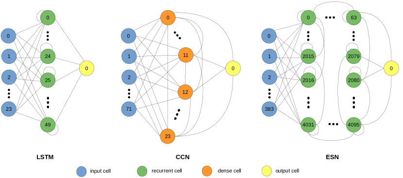
Figure 3: Flowchart Diagrams Depicting our Deep Learning Model Architecture Configurations for AQD.

3.5.2 HPC

Our model is developed with one hidden LSTM recurrent layer with 200 neurons. The second layer is fully connected with 200 neurons. Lastly, the direct forecast is produced by an output layer that outputs a vector with seven entries, as previously described. Our model is trained for 65 epochs with a batch size of 18, determined experimentally to be optimal.

The ESN uses a $28$ day wash-out interval. The CCN has seven neurons in the output layer, with cascading capped at $28$ layers.

The first three calendar years are used as training data and the final year for model evaluation purposes.

3.5.3 BSD

The LSTM is initialized with 100 neurons in the sole hidden recurrent layer, followed by an output layer that directly forecasts a vector with seven days worth of forecasts. We fit the model for $25$ epochs with a batch size of $32$.

The ESN uses a seven day wash-out interval. The CCN has $168$ neurons in the output layer, with cascading capped at $28$ layers.

3.5.4 BDS

We instantiate the LSTM with 100 neurons in the input layer, one hidden recurrent layer with 50 neurons, and an output layer comprised of 4 neurons. Our model is fit for 100 epochs with a batch size of 32.

The ESN is initialized with $48$ input units, $4$ output units, and $1,024$ internal network units in the dynamic reservoir. We use a $24$ hour wash-out interval.

The CCN is composed of $100$ neurons in the input layer and $4$ neurons in the output layer. The cascading is capped at $24$ layers.

3.5.5 YWB

The LSTM has 5 hidden layers with 4, 16, 48, 16, and 4 neurons, respectively. Our model is fit for 45 epochs with a batch size of 24.

The ESN uses a $3$ day wash-out interval. The CCN has $4$ neurons in the output layer, with cascading capped at $9$ layers.

3.5.6 Overall

In terms of AQD, we use holdout cross-validation, fitting each of the models on the first four years of data and testing with the remaining year. For all the other datasets, we use walk-forward validation for optimizing the hyper-parameters. For instance, with HPC, our models forecast a week ahead $\hat{y}_{t+1}$. After that, the actual observations from a week ahead $y_{t+1}$ are presented to the models, and are used in the set of observations $\ldots y_{t-2},y_{t-1},y_{t},y_{t+1}$ for the current iteration in the walk-forward validation process, before we forecast the subsequent week $\hat{y}_{t+2}$.

As an additional method to mitigate computational cost, the models are evaluated statically, i.e. they are trained on the historical observations and then iteratively forecast each step of the walk-forward validation.

For each architecture, we use the Mean Absolute Error (MAE, Sammut and Webb (2010)) loss function and the efficient Adam version of stochastic gradient descent Kingma and Ba (2014). Each configuration was selected over various others based on empirical studies of test RMSE reduction and configuration behaviour over time.

The input variables to VARMAX and SARIMAX are declared as exogenous.

After each model is fit, we forecast, replace the seasonality and trend components, invert the scaling, and compute an error score for each. The results follow in Section 4.1.

3.6 Evaluation

The LSTM is implemented using the LSTM and Dense class of the Keras API v2.1.5 (Chollet et al., 2015) for Python 3.7 using TensorFlow v1.15.0 framework as backend (Abadi et al., 2016). The code implementation for the CCN is written from scratch using Python 3.7, and ESN is implemented using PyTorch v0.3 (Paszke et al., 2017) for Python 3.7. The naïve or benchmark methods are implemented using the Statsmodels API Seabold and Perktold (2010) for Python 3.7. All models are trained on an Intel Core i7-9750H processor with an Nvidia GeForce GTX 1650 GPU.

3.7 Recurrent Layer Dropout

We compare the forecast accuracy at dropout rates of $15\%$, $30\%$, $45\%$, and $60\%$ to the standard LSTM fit above (i.e. with no dropout). Each dropout experiment is repeated $35$ times to mitigate the stochastic nature of the deep learning algorithms. Table 4, and the box and whisker plot in Figure 4, display the distributions of results for each configuration in the case of AQD as an illustrative example.

Table 4: Dropout RMSE Score Distributions.

	Dropout Rate
	0.0	0.15	0.3	0.45	0.6
count	35	35	35	35	35
mean	20.7746	21.8681	22.5086	23.7820	25.4886
std	0.0000	0.1283	0.1793	0.2436	0.2812
min	20.7746	21.5665	22.2587	23.4037	24.8913
25%	20.7746	21.8193	22.4969	23.5335	25.2295
50%	20.7746	21.8543	22.5990	23.7627	25.4671
75%	20.7746	21.9773	22.7260	23.8939	25.6549
max	20.7746	22.0783	22.9699	24.3575	25.8718

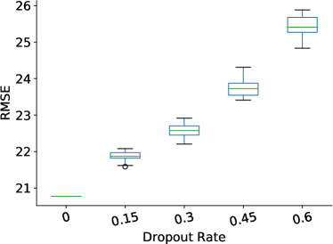
Figure 4: Dropout RMSE Score Distributions.

From Table 4, we note that the standard implementation (LSTM with no dropout) outperforms all the configurations with dropout. At $15\%$ the output has the tightest distribution (a desirable property for constructing prediction intervals). The $15\%$ dropout configuration has a competitive RMSE compared to the standard implementation. Because we drop out at such a low probability, this configuration retains a lot more information than the others. We thus use this configuration for prediction interval construction.

We run the chosen configuration $100,000$ times. In this case, the $15\%$ dropout probability. We forecast, and use the distribution of said forecast values to construct our prediction intervals. To compute the $(1-\alpha)\times 100\%$ prediction interval, we use the percentiles at

$$\left(\dfrac{\alpha}{2},\left(1-\alpha\right)+\left(\dfrac{\alpha}{2}\right)\right)$$

.

3.8 Bootstrap

We resample residuals in the following manner:

1. Once the model is fit, retain the values fitted, $y^{\prime}_{t}$, and residuals $\varepsilon_{t}=y_{t}-y^{\prime}_{t},t=1,\dots,m$, where $m\leq n$ our forecast horizon.

2. For each tuple, $\left(\vec{x}_{t},y_{t}\right)$, in which $\vec{x}_{t}$ is the multivariate explanatory variable, add the randomly resampled residual, $\varepsilon_{j}$, to the fitted value $y^{\prime}_{t}$, thus creating synthetic response variables $y^{*}_{t}=y^{\prime}_{t}+\varepsilon_{j}$ where $j$ is selected randomly from the list $\left(1,...,m\right)$ for every $t$.

3. Using the values $\left(\vec{x}_{t},y^{*}_{t}\right)$, forecast $\hat{y}$, then refit the model using synthetic response variables $y^{*}_{t}$, again retaining the residuals and forecasts.

4. Repeat steps 2 and 3, $100,000$ times.

We use the distribution of the forecast values to construct the prediction intervals using percentiles in the same manner described in Section 3.7 above. As in the case of the recurrent layer dropout, this technique is advantageous as it retains the explanatory variables’ information.

3.9 Anomaly Detection

Anomalies are labeled in YWB. BDS does not contain any golden labels. We synthesize anomalies by superimposing them on the other three datasets, as previously mentioned in Section 2.5 above. This step is undertaken in a stochastic manner, where a typical composition is given in Table 5.

Table 5: Anomaly Data Structure Summary.

Data	# Metrics	Type	Contamination
AQD	$10$	changepoint	$0.0133$
HPC	$7$	collective	$0.0142$
BSD	$17$	contextual	$0.0209$
BDS	$36$	changepoint	$0.0191$
YWB	$67$	contextual & collective	$0.0176$

If a new observation falls within our constructed prediction interval, it is classified as normal. If it falls outside the interval, we:

1. determine by which magnitude it falls outside the bounds. This measure is deducible using a variant of MIS defined earlier (Equation 3 in Section 3.4), i.e. the Interval Score (IS)

   $$\qquad\text{IS}_{\alpha} =\left(U_{t}-L_{t}\right)+\dfrac{2}{\alpha}\left(L_{t}-y_{t}\right)\mathbb{1}_{\left\{y_{t}<L_{t}\right\}}$$

   $$\qquad~{}+\dfrac{2}{\alpha}\left(y_{t}-U_{t}\right)\mathbb{1}_{\left\{y_{t}>U_{t}\right\}}$$

   If this measure is at least $33\%$ larger than that of the previous observation that fell outside bounds, then we

2. employ Chebyshev’s inequality Dixon and Massey (1968) which guarantees a useful property for a wide class of probability distributions, i.e. no more than a certain fraction of values can be more than a certain distance from the mean. A suitable threshold can be tuned to avoid many false alerts. In our case, we utilize this inequality to identify that $99\%$ of the values must lie within ten times the standard deviation.

If an out-of-sample observation falls outside the prediction interval bounds and falls beyond ten times the standard deviation of the observations (our dynamic threshold, $\leq 1\%$ of all observations), it is classified as anomalous.

Essentially, the anomaly detection procedure may be summarized in Algorithm 1, and the entire structure of our deep learning models and data flow process is presented graphically in Figure 5.

Algorithm 1 Anomaly Detection

  if $U_{t}\leq y_{t}\leq L_{t}$ then

     $y_{t}$ is normal

  else

     if $\text{IS}_{\alpha}\left(y_{t}\right)\geq 1.33\times\text{IS}_{\alpha}\left(y_{*}\right)$ and $y_{t}>10\times\text{std}{\left\{\dots,y_{t-3},y_{t-2},y_{t-1}\right\}}$ then

        $y_{t}$ is anomalous {where $y_{*}$ is the last anomalous observation}

     end if

  end if

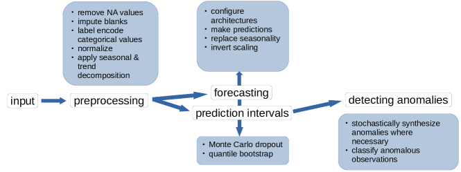
Figure 5: Flowchart Diagram Depicting our Deep Learning Model Architectures.

4 Results

4.1 Forecasting

A persistence model Coimbra and Pedro (2013) gives an RMSE score of $30$, $465$, $94$, $1.8$, and $301$ respectively for AQD, HPC, BSD, BDS and YWB. Those from the models under consideration, truncated to four decimals, are shown in Table 6.

Table 6: Model Error Scores.

Data AQD HPC BSD BDS YWB Statistical Benchmarks MLR 24.8791 415.8602 43.8581 1.5001 278.6595 SARIMAX 22.9377 377.8571 34.3472 1.3712 251.8902 VARMAX 23.1093 401.3319 39.2279 1.4879 266.0144 Deep Learning LSTM 20.1342 337.9452 31.8951 0.9588 213.8532 ESN 21.2357 349.1773 31.0451 1.0057 209.3517 CCN 22.9876 392.5459 35.6843 1.1421 227.1096

4.2 Prediction Intervals

For ease of interpretation, we modify the MIS to introduce a scaling factor, such that the best performing model has scaled Mean Interval Score (sMIS) equal to $1$, and the rest are larger than $1$. The worst performing model thus has the largest sMIS value. For each significance level $\alpha$ considered we have,

$$\text{sMIS}_{\alpha,i} =\dfrac{\text{MIS}_{\alpha,i}}{\min\limits_{i\in X}\text{MIS}_{\alpha,i}},$$ (6)

where $X$ comprises all algorithms considered (both statistical and deep learning). We further highlight the top two performers at each significance level.

Table 7: Prediction Interval Performance for Air Quality Data.

sMIS $\alpha$ CS $\alpha$ 0.1 0.05 0.01 0.1 0.05 0.01 MLR 1.1704 1.2105 1.2323 0.9031 0.9171 0.9305 SARIMAX Gray1.0778 1.2093 1.2167 Gray 0.9524 Gray 0.9668 Gray 0.9797 Statistical Bench- marks VARMAX 1.4141 1.2662 1.0881 0.9449 0.9621 0.9761 LSTM Gray 1.0000 1.1437 Gray 1.0000 Gray 0.9620 Gray 0.9810 Gray 0.9824 ESN 1.1859 Gray 1.1365 1.1367 0.9179 0.9308 0.9435 Deep Learning CCN 1.2103 Gray 1.0000 Gray 1.0655 0.9094 0.9285 0.9633

Table 8: Prediction Interval Performance for Bike Sharing Data.

sMIS $\alpha$ CS $\alpha$ 0.1 0.05 0.01 0.1 0.05 0.01 MLR 1.2131 1.1688 1.2072 0.9062 0.9169 0.9165 SARIMAX 1.0364 1.2052 1.2708 Gray0.9493 0.9501 Gray0.9553 Statistical Bench- marks VARMAX 1.1236 1.1796 1.1676 0.9075 0.9107 0.9194 LSTM 1.1727 1.0872 1.1662 0.9370 Gray0.9519 0.9422 ESN Gray1.0000 Gray1.0000 Gray1.0000 Gray0.9587 Gray0.9683 Gray0.9772 Deep Learning CCN Gray1.0186 Gray1.0388 Gray1.0409 0.9468 0.9472 0.9495

Table 9: Prediction Interval Performance for Household Power Consumption Data.

sMIS $\alpha$ CS $\alpha$ 0.1 0.05 0.01 0.1 0.05 0.01 MLR 1.2262 1.2123 1.1686 0.9081 0.9117 0.9144 SARIMAX 1.1081 Gray1.0181 1.1012 Gray0.9413 0.9514 0.9760 Statistical Bench- marks VARMAX 1.1764 1.1565 1.1148 0.9178 0.9262 0.9322 LSTM Gray1.0449 1.1005 Gray1.0211 Gray0.9507 Gray0.9594 Gray0.9767 ESN 1.0910 Gray1.0000 Gray1.0000 0.9372 Gray0.9516 Gray0.9895 Deep Learning CCN Gray1.0000 1.1452 1.0708 0.9157 0.9299 0.9571

Table 10: Prediction Interval Performance for Bearings Data.

sMIS $\alpha$ CS $\alpha$ 0.1 0.05 0.01 0.1 0.05 0.01 MLR 1.3562 1.2020 1.1549 0.9106 0.9134 0.9287 SARIMAX Gray1.0000 1.1254 1.1832 0.8957 0.9009 0.9071 Statistical Bench- marks VARMAX 1.1764 1.1565 1.2149 0.9075 0.9161 0.9193 LSTM Gray1.0541 1.1045 Gray1.0299 Gray0.9401 Gray0.9412 Gray0.9491 ESN 1.0910 Gray1.0000 Gray1.0000 0.9202 Gray0.9346 Gray0.9398 Deep Learning CCN 1.1081 Gray1.0181 1.1012 Gray0.9213 0.9277 0.9301

Table 11: Prediction Interval Performance for Webscope Benchmark Data.

sMIS $\alpha$ CS $\alpha$ 0.1 0.05 0.01 0.1 0.05 0.01 MLR 1.3054 1.112 1.1499 0.8878 0.8923 0.8971 SARIMAX 1.1081 Gray1.0169 1.1012 Gray0.9293 0.9313 0.9360 Statistical Bench- marks VARMAX 1.2262 1.2123 1.1686 0.8981 0.9108 0.9142 LSTM 1.0812 Gray1.0000 Gray1.0000 0.9271 Gray0.9360 Gray0.9494 ESN Gray1.0546 1.1050 Gray1.0233 Gray0.9307 Gray0.9394 Gray0.9464 Deep Learning CCN Gray1.0000 1.1452 1.0708 0.9157 0.9299 0.9309

Tables 7 to 11 detail the prediction interval results. We note that at least one deep learning algorithm is always in the top two performers. The interpretation is that deep learning algorithms outperform the traditional statistical methods, or at the very least, are competitive. This outperformance is also evidenced by the granular result for aggregated daily RMSE for HPC, as displayed in Figure 6. Figure 6 is supplementary to Table 9 as it gives a granular score at a daily level, which is consistent with the overall score detailed in the latter. Figure 7 illustrates the point forecasts and prediction intervals for ESN (best performer for BSD) at the last $120$ hours of our forecast horizon. Our results are consistent with the findings of Makridakis et al. (2020b), who noted that deep learning models produce better prediction intervals, albeit in the univariate case.

ESN is the best performing architecture for the BSD at the all prediction intervals considered. This result is consistent with the RMSE scores in Table 6.

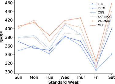
Figure 6: Overall Daily RMSE for Household Power Consumption Dataset.

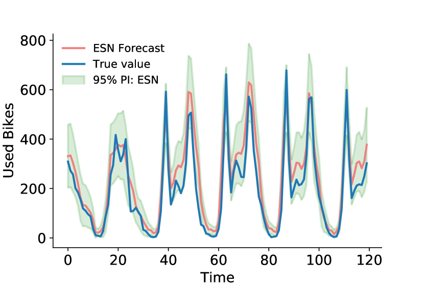
Figure 7: Point Forecasts and Prediction Intervals for Bike Sharing Dataset.

4.3 Anomaly Detection

Figures 8 and 9 detail the distributions for the $F_{1}$- and $Ed$-scores, respectively, for all the models applied to each dataset. We note the $F_{1}$-score is varied for each dataset, but the results indicate LSTM is the best performer, followed in every instance by either ESN or CCN. The worst performer is MLR across all datasets. Since the $F_{1}$-score is the harmonic average of Precision and Recall, where $1$ is the perfect score and $0$ is worst, we note that the deep learning models are better at learning the dynamic threshold.

Again, with the $Ed$-score, the statistical methods are outperformed by the deep learning models. This result follows as better dynamic threshold calibration leads to earlier detection of anomalies.

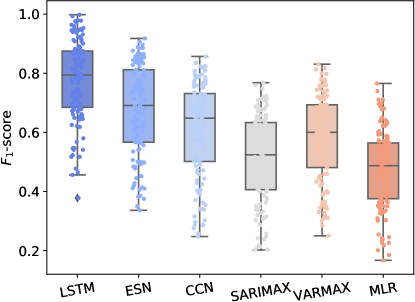
(a) $F_{1}$-Score for AQD.

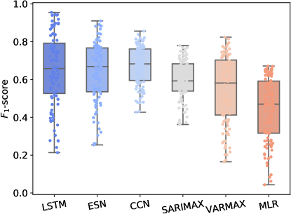
(b) $F_{1}$-Score for BSD.

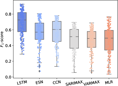
(c) $F_{1}$-Score for HPC.

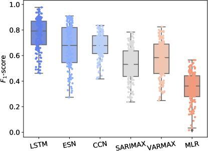
(d) $F_{1}$-Score for BDS.

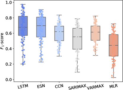
(e) $F_{1}$-Score for YWB.

Figure 8: $F_{1}$-Score distribution for each datasets and all the models.

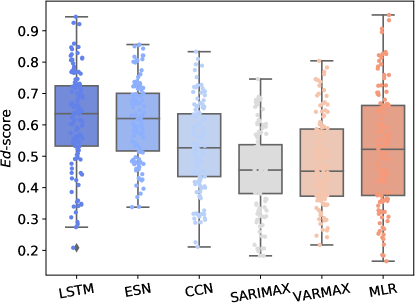
(a) $Ed$-Score for AQD.

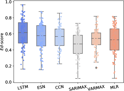
(b) $Ed$-Score for BSD.

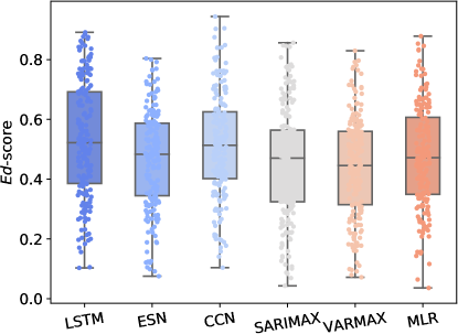
(c) $Ed$-Score for HPC.

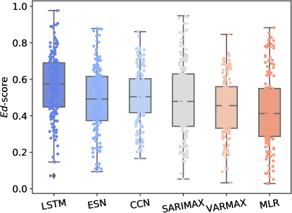
(d) $Ed$-Score for BDS.

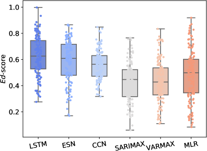
(e) $Ed$-Score for YWB.

Figure 9: $Ed$-Score distribution for each datasets and all the models.

5 Conclusion

Our point of departure is that $(i)$ deep learning models have been shown to outperform traditional statistical methods at forecasting, and $(ii)$ deep learning has been shown to produce superior uncertainty quantification. In this paper, we $(i)$ produce point forecasts, $(ii)$ produce their associated prediction intervals using computational means where no built-in probabilistic constructs exist, and $(iii)$ use said prediction intervals to detect anomalies on different multivariate datasets.

With the methodology presented, we note that better point forecast accuracy leads to the construction of better prediction intervals, which in turn leads to the main result presented: better prediction intervals lead to more accurate and faster anomaly detection. The improvement is as a result of better parameterized models being capable of more accurate forecasts. These models in turn are used in the interval construction process and subsequently multivariate anomaly detection.

The goal was not to prove that deep learning is far superior to statistical methods in this regard, but to show that when proper methodology is followed, it can be competitive in the worst case. This in an important result, as it opens the way for the wide-scale adoption of deep learning in other applications.

The computational cost of the deep learning algorithms is not discussed in this paper and this could be an avenue for further exploration. The algorithmic time complexity is known for each model, with ESN being the fastest deep learning architecture. Even at that, it is still not as fast as any of the statistical methods. In terms of the deep learning architectures, future work can consider techniques for improving upon the cost of computation, so that even in this aspect they become competitive to their statistical counterparts.

Finding techniques to address this last issue in particular, will enable researchers to study multivariate time series in more detail, and at a grander scale. There exists a need for conducting our kind of analysis on multivariate time series at the scale of, say, the M4 competition Makridakis et al. (2020b).

Conflict of Interest

The authors declare that they have no conflict of interest.

References

- Abadi et al. (2016) Martín Abadi, Paul Barham, Jianmin Chen, Zhifeng Chen, Andy Davis, Jeffrey Dean, Matthieu Devin, Sanjay Ghemawat, Geoffrey Irving, Michael Isard, Manjunath Kudlur, Josh Levenberg, Rajat Monga, Sherry Moore, Derek G. Murray, Benoit Steiner, Paul Tucker, Vijay Vasudevan, Pete Warden, Martin Wicke, Yuan Yu, and Xiaoqiang Zheng. Tensorflow: A system for large-scale machine learning. In Proceedings of the 12th USENIX Conference on Operating Systems Design and Implementation, OSDI’16, pages 265–283, Berkeley, CA, USA, 2016. USENIX Association. ISBN 978-1-931971-33-1. URL https://www.usenix.org/system/files/conference/osdi16/osdi16-abadi.pdf.
- Adewumi and Akinyelu (2016) Aderemi O. Adewumi and Andronicus A. Akinyelu. A survey of machine-learning and nature-inspired based credit card fraud detection techniques, international journal of system assurance engineering and management. International Journal of System Assurance Engineering and Management, 8(2):937–953, 2016. ISSN 0976-4348, 0975-6809. URL https://doi.org/10.1007/s13198-016-0551-y.
- Aggarwal (2013) Charu C. Aggarwal. Probabilistic and statistical models for outlier detection. In Outlier Analysis, chapter 2, pages 41–74. Springer, New York, NY, 2013. URL https://doi.org/10.1007/978-1-4614-6396-2_2.
- Arunraj et al. (2016) Nari Arunraj, Diane Ahrens, and Michael Fernandes. Application of SARIMAX model to forecast daily sales in food retail industry. International Journal of Operations Research and Information Systems, 7:1–21, 04 2016. URL https://doi.org/10.4018/IJORIS.2016040101.
- Brink et al. (2016) Henrik Brink, Joseph Richards, and Mark Fetherolf. Scaling machine-learning workflows. In Real-World Machine Learning, chapter 9. Manning Publications Co., New York, NY, 2016. URL https://livebook.manning.com/book/real-world-machine-learning/chapter-9/8.
- Buda et al. (2017) T. S. Buda, H. Assem, and L. Xu. Ade: An ensemble approach for early anomaly detection. In 2017 IFIP/IEEE Symposium on Integrated Network and Service Management (IM), pages 442–448, 2017. URL https://www.researchgate.net/publication/318664756_ADE_An_ensemble_approach_for_early_Anomaly_Detection.
- Carreńo et al. (2020) Ander Carreńo, Ińoaki Inza, and Jose Lozano. Analyzing rare event, anomaly, novelty and outlier detection terms under the supervised classification framework. Artificial Intelligence Review, 53:3575–3594, 06 2020. URL https://doi.org/10.1007/s10462-019-09771-y.
- Chauhan and Vig (2015) Sucheta Chauhan and Lovekesh Vig. Anomaly detection in ecg time signals via deep long short-term memory networks. pages 1–7, 10 2015. URL https://doi.org/10.1109/DSAA.2015.7344872.
- Chen (2014) Song Xi Chen. UCI machine learning repository Beijing PM2.5 data set. http://archive.ics.uci.edu/ml/datasets/Beijing+PM2.5+Data, 2014. [Online; accessed 12-February-2020].
- Chollet et al. (2015) François Chollet et al. Keras. https://keras.io, 2015.
- Claveria et al. (2015) Oscar Claveria, Enric Monte, and Salvador Torra. Effects of removing the trend and the seasonal component on the forecasting performance of artificial neural network techniques. Working Paper 2015/031/16, Research Institute of Applied Economics, Spain, 2015. URL https://doi.org/10.13140/RG.2.2.27306.21447.
- Cleveland et al. (1990) Robert B. Cleveland, William S. Cleveland, Jean E. McRae, and Irma Terpenning. STL: A seasonal-trend decomposition procedure based on LOESS (with discussion). Journal of Official Statistics, 6:3–73, 1990. URL http://www.ccpo.odu.edu/~klinck/Reprints/PaperWebPages/clevelandJOffStat1990.html.
- Coimbra and Pedro (2013) Carlos F.M. Coimbra and Hugo T.C. Pedro. Chapter 15 - Stochastic-learning Methods. In Jan Kleissl, editor, Solar Energy Forecasting and Resource Assessment, pages 383–406. Academic Press, Boston, 2013. ISBN 978-0-12-397177-7. URL https://doi.org/10.1016/B978-0-12-397177-7.00015-2.
- Davison and Hinkley (2013) A. C. Davison and D. V. Hinkley. Bootstrap Methods and Their Application. Cambridge University Press, USA, 2013. ISBN 0511802846. URL https://dl.acm.org/doi/book/10.5555/2556084.
- Dixon and Massey (1968) W. J. Dixon and Frank J. Massey. Introduction to statistical analysis. McGraw-Hill New York, 3d ed. edition, 1968. URL https://nla.gov.au/nla.cat-vn645066.
- Fahlman and Lebiere (1990) Scott E. Fahlman and Christian Lebiere. The cascade-correlation learning architecture. In Advances in Neural Information Processing Systems 2, pages 524–532. Morgan Kaufmann, 1990. URL https://doi.org/10.1007/978-1-4899-7687-1_33.
- Fanaee-T and Gama (2012) Hadi Fanaee-T and Joao Gama. UCI machine learning repository bike sharing data set. https://archive.ics.uci.edu/ml/datasets/bike+sharing+dataset, 2012. [Online; accessed 05-June-2020].
- Gal (2016) Yarin Gal. Uncertainty in Deep Learning. PhD thesis, University of Cambridge, 2016. URL https://mlg.eng.cam.ac.uk/yarin/thesis/thesis.pdf.
- Gal and Ghahramani (2016) Yarin Gal and Zoubin Ghahramani. Dropout as a Bayesian approximation: Representing model uncertainty in deep learning. In Proceedings of the 33rd International Conference on International Conference on Machine Learning, volume 48 of ICML’16, pages 1050–1059. JMLR.org, 2016. URL http://proceedings.mlr.press/v48/gal16.pdf.
- Gneiting and Raftery (2007) Tilmann Gneiting and Adrian E. Raftery. Strictly proper scoring rules, prediction, and estimation. Journal of the American Statistical Association, 102(477):359–378, 2007. URL https://doi.org/10.1198/016214506000001437.
- Hannan and Deistler (1992) E. J. Hannan and Manfred Deistler. The statistical theory of linear systems. Econometric Theory, 8(1):135–143, 1992. URL https://doi.org/10.1017/S026646660001080X.
- Hawkins (1980) D. M. Hawkins. Identification of outliers. Monographs on applied probability and statistics. Chapman and Hall, 1980. ISBN 041221900X. URL https://doi.org/10.1002/bimj.4710290215.
- Hebrail and Berard (2012) Georges Hebrail and Alice Berard. UCI machine learning repository individual household electric power consumption data set. https://archive.ics.uci.edu/ml/datasets/individual+household+electric+power+consumption, 2012. [Online; accessed 01-June-2020].
- Hesterberg (2014) Tim Hesterberg. What teachers should know about the bootstrap: Resampling in the undergraduate statistics curriculum, 2014. URL https://arxiv.org/abs/1411.5279.
- Hochreiter and Schmidhuber (1997) Sepp Hochreiter and Jürgen Schmidhuber. Long short-term memory. Neural computation, 9(8):1735–1780, 1997. URL https://doi.org/10.1162/neco.1997.9.8.1735.
- Jaeger (2001) Herbert Jaeger. The ”Echo State” approach to analysing and training recurrent neural networks. GMD Report 148, GMD - German National Research Institute for Computer Science, 2001. URL http://www.faculty.jacobs-university.de/hjaeger/pubs/EchoStatesTechRep.pdf.
- Kingma and Ba (2014) Diederik P. Kingma and Jimmy Ba. Adam: A method for stochastic optimization, 2014. URL http://arxiv.org/abs/1412.6980. 3rd International Conference for Learning Representations, San Diego, 2015.
- Kwon et al. (2019) Donghwoon Kwon, Hyunjoo Kim, Jinoh Kim, Sang Suh, Ikkyun Kim, and Kuinam Kim. A survey of deep learning-based network anomaly detection. Cluster Computing, 22, 01 2019. URL https://doi.org/10.1007/s10586-017-1117-8.
- Laptev and Amizadeh (2015) N Laptev and S Amizadeh. Yahoo webscope benchmark dataset. http://webscope.sandbox.yahoo.com/catalog.php, 2015. [Online; accessed 29-October-2020].
- Lee et al. (2007) J Lee, H Qiu, G Yu, J Lin, and Rexnord Technical Services. NASA Ames prognostics data repository. https://ti.arc.nasa.gov/tech/dash/groups/pcoe/prognostic-data-repository/#bearing, 2007. [Online; accessed 13-October-2020].
- Li et al. (2017) Jinbo Li, Witold Pedrycz, and Iqbal Jamal. Multivariate time series anomaly detection: A framework of hidden markov models. Applied Soft Computing, 60:229 – 240, 2017. ISSN 1568-4946. doi: https://doi.org/10.1016/j.asoc.2017.06.035. URL http://www.sciencedirect.com/science/article/pii/S1568494617303782.
- Makridakis et al. (2020a) Spyros Makridakis, Rob J. Hyndman, and Fotios Petropoulos. Forecasting in social settings: The state of the art. International Journal of Forecasting, 36(1):15 – 28, 2020a. ISSN 0169-2070. URL https://doi.org/10.1016/j.ijforecast.2019.05.011.
- Makridakis et al. (2020b) Spyros Makridakis, Evangelos Spiliotis, and Vassilios Assimakopoulos. The M4 Competition: 100,000 time series and 61 forecasting methods. International Journal of Forecasting, 36(1):54–74, 2020b. URL https://doi.org/10.1016/j.ijforecast.2019.04.014.
- Malhotra et al. (2015) Pankaj Malhotra, Lovekesh Vig, Gautam Shroff, and Puneet Agarwal. Long short term memory networks for anomaly detection in time series. In European Symposium on Artificial Neural Networks, Computational Intelligence and Machine Learning (ESANN), pages 89–94, 2015. URL https://www.elen.ucl.ac.be/Proceedings/esann/esannpdf/es2015-56.pdf.
- Malhotra et al. (2016) Pankaj Malhotra, Anusha Ramakrishnan, Gaurangi Anand, Lovekesh Vig, Puneet Agarwal, and Gautam Shroff. Lstm-based encoder-decoder for multi-sensor anomaly detection. CoRR, abs/1607.00148, 2016. URL http://arxiv.org/abs/1607.00148.
- Mathonsi and van Zyl (2020) T. Mathonsi and T. L. van Zyl. Prediction interval construction for multivariate point forecasts using deep learning. In 2020 7th International Conference on Soft Computing Machine Intelligence (ISCMI), pages 88–95, 2020. URL https://doi.org/10.1109/ISCMI51676.2020.9311603.
- Matthews (2005) David E. Matthews. Multiple Linear Regression, chapter 5, pages 119–133. American Cancer Society, 2005. ISBN 9780470011812. URL https://doi.org/10.1002/0470011815.b2a09033.
- Mullachery et al. (2018) Vikram Mullachery, Aniruddh Khera, and Amir Husain. Bayesian neural networks. CoRR, abs/1801.07710, 2018. URL http://arxiv.org/abs/1801.07710.
- Paszke et al. (2017) Adam Paszke, Sam Gross, Soumith Chintala, Gregory Chanan, Edward Yang, Zachary DeVito, Zeming Lin, Alban Desmaison, Luca Antiga, and Adam Lerer. Automatic differentiation in PyTorch. In NIPS 2017 Workshop Autodiff, 2017. URL https://openreview.net/pdf?id=BJJsrmfCZ.
- Pedregosa et al. (2011) F. Pedregosa, G. Varoquaux, A. Gramfort, V. Michel, B. Thirion, O. Grisel, M. Blondel, P. Prettenhofer, R. Weiss, V. Dubourg, J. Vanderplas, A. Passos, D. Cournapeau, M. Brucher, M. Perrot, and E. Duchesnay. Scikit-learn: Machine learning in Python. Journal of Machine Learning Research, 12:2825–2830, 2011. URL https://arxiv.org/pdf/1201.0490.pdf.
- Prosvirin et al. (2017) Alexander Prosvirin, M M Manjurul Islam, Cheolhong Kim, and Jongmyon Kim. Fault prediction of rolling element bearings using one class least squares SVM. In Proceedings of the Engineering and Arts Society in Korea, volume 15, pages 93–96, 12 2017. URL https://www.researchgate.net/publication/321906715_Fault_Prediction_of_Rolling_Element_Bearings_Using_One_Class_Least_Squares_SVM.
- Sammut and Webb (2010) Claude Sammut and Geoffrey I. Webb, editors. Mean Absolute Error, pages 652–652. Springer US, Boston, MA, 2010. ISBN 978-0-387-30164-8. URL https://doi.org/10.1007/978-0-387-30164-8_525.
- Schlegl et al. (2017) Thomas Schlegl, Philipp Seeböck, Sebastian M. Waldstein, Ursula Schmidt-Erfurth, and Georg Langs. Unsupervised anomaly detection with generative adversarial networks to guide marker discovery. CoRR, abs/1703.05921, 2017. URL http://arxiv.org/abs/1703.05921.
- Schölkopf et al. (1999) Bernhard Schölkopf, Robert Williamson, Alex Smola, John Shawe-Taylor, and John Platt. Support vector method for novelty detection. In Proceedings of the 12th International Conference on Neural Information Processing Systems, NIPS’99, pages 582–588, Cambridge, MA, USA, 1999. MIT Press. URL https://papers.nips.cc/paper/1999/file/8725fb777f25776ffa9076e44fcfd776-Paper.pdf.
- Seabold and Perktold (2010) Skipper Seabold and Josef Perktold. statsmodels: Econometric and statistical modeling with Python. In 9th Python in Science Conference, 2010. URL https://conference.scipy.org/proceedings/scipy2010/pdfs/seabold.pdf.
- Sivarajah et al. (2017) Uthayasankar Sivarajah, Muhammad Mustafa Kamal, Zahir Irani, and Vishanth Weerakkody. Critical analysis of big data challenges and analytical methods. Journal of Business Research, 70:263–286, 2017. ISSN 0148-2963. URL https://doi.org/10.1016/j.jbusres.2016.08.001.
- Smyl (2020) Slawek Smyl. A hybrid method of exponential smoothing and recurrent neural networks for time series forecasting. International Journal of Forecasting, 36(1):75–85, 2020. ISSN 0169-2070. doi: https://doi.org/10.1016/j.ijforecast.2019.03.017. URL https://www.sciencedirect.com/science/article/pii/S0169207019301153. M4 Competition.
- Thi et al. (2018) Nga Nguyen Thi, Van Loi Cao, and Nhien-An Le-Khac. One-class collective anomaly detection based on long short-term memory recurrent neural networks. CoRR, abs/1802.00324, 2018. URL http://arxiv.org/abs/1802.00324.
- Thill et al. (2017) M. Thill, W. Konen, and T. Bäck. Online anomaly detection on the webscope s5 dataset: A comparative study. In 2017 Evolving and Adaptive Intelligent Systems (EAIS), pages 1–8, 2017. URL https://ieeexplore.ieee.org/document/7954844.
- Thudumu et al. (2020) Srikanth Thudumu, Philip Branch, Jiong Jin, and Jugdutt Singh. A comprehensive survey of anomaly detection techniques for high dimensional big data. Journal of Big Data, 42:7–37, 2020. URL https://doi.org/10.1186/s40537-020-00320-x.
- Williams and Zipser (1989) Ronald J. Williams and David Zipser. A learning algorithm for continually running fully recurrent neural networks. Neural Computation, 1(2):270–280, 1989. ISSN 0899-7667. URL https://doi.org/10.1162/neco.1989.1.2.270.
- Zhu and Laptev (2017) Lingxue Zhu and Nikolay Laptev. Deep and Confident Prediction for Time Series at Uber. ArXiv e-prints, 2017. URL https://doi.org/10.1109/ICDMW.2017.19.