Limit of trees with fixed degree sequence

Abstract

We use a new stick-breaking construction, also introduced independently by Addario-Berry, Donderwinkel, Maazoun, and Martin in [28], to study uniform rooted trees with fixed degree sequence $\mathcal{D}$ ($\mathcal{D}$-trees). This construction allows us to prove, under natural conditions of convergence of the degree sequence, that $\mathcal{D}$-trees converge toward either $\mathcal{P}$-trees or ICRT. Alongside we provide an upper-bound for the height of $\mathcal{D}$-trees. We deduce similar results concerning $\mathcal{P}$-trees and ICRT. In passing we confirm a conjecture of Aldous, Miermont, and Pitman [7] stating that Lévy trees are ICRT with random parameters.

1 Introduction

1.1 Overview of the results

Let $\{V_{i}\}_{i\in\mathbb{N}}$ be a set of vertices. A rooted tree $T$ is said to have degree sequence $(d_{i})_{1\leq i\leq s}$ if $T$ has vertices $\{V_{i}\}_{1\leq i\leq s}$ and for every $1\leq i\leq s$, $V_{i}$ has $d_{i}$ children.

The aim of this paper is to study $\mathcal{D}$-trees: uniform rooted trees with fixed degree sequence $\mathcal{D}$. Notably we show, under natural conditions of convergence of the degree sequence, that $\mathcal{D}$-trees converge either toward $\mathcal{P}$-trees, or after normalisation by $s/\sqrt{\sum_{i=1}^{s}d_{i}(d_{i}-1)}$ toward ICRT, for the Gromov–Prokhorov (GP) topology. Furthermore we show, under a given tightness assumption, that $\mathcal{D}$-trees also converge toward ICRT for the Gromov–Hausdorff–Prokhorov (GHP) topology. Alongside we provide a near optimal upper bound for the height of $\mathcal{D}$-trees.

Those results are in direct continuity with the work of Aldous, Camarri, Pitman [8, 19], which proves that $\mathcal{P}$-trees converge toward ICRT for the GP topology. We also complete their results by considering the GHP topology, and by proving an upper bound for the height of $\mathcal{P}$-trees and ICRT.

When taken together, those results on $\mathcal{D}$-trees, $\mathcal{P}$-trees and ICRT can be used to study the different models of trees that are uniform when conditioned to their exact degree sequence (see the end of the introduction and Section 8.1 for more details).

Finally, this paper is simplified thanks to the results of a companion paper [12], which introduces and studies a new construction for ICRT. Notably, the probability measure introduced in [12] and the compactness of ICRT avoid us many computations and topological arguments.

1.2 Overview of the proof

Our approach relies on a new construction for $\mathcal{D}$-trees, which can be seen in three different ways: as a modification of Aldous–Broder algorithm, as a recursive construction of subtrees spanned by specific leaves, and as a stick-breaking construction. Our proof is strongly based on those points of view so let us recall them: (see also Figure 1 for a construction)

• (a) Aldous–Broder algorithm: Fix an arbitrary random walk $(A_{i})_{i}$. Start with a single vertex $A_{1}$, then recursively add the edge $\{A_{i-1},A_{i}\}$ when $A_{i}$ is "new", that is when $A_{i}\notin\{A_{j}\}_{j<i}$. It is well known, since its introduction in [4, 14], that this algorithm yields a random tree. Along the construction, we add an edge between $A_{i-1}$ and a new leaf when $A_{i}$ is not "new". By doing so, the number of children of a vertex equals the number of times it is visited. Moreover we show that if $(A_{i})_{i}$ is uniform among all $\mathcal{D}$-tuple, that is tuple such that for every $i\in\mathbb{N}$ $V_{i}$ appears $d_{i}$ times, then this algorithm constructs a $\mathcal{D}$-tree.

• (b) Subtrees spanned by specific leaves: Note that the last algorithm, when stopped at the $k^{th}$ repetition ($k^{th}$ index such that $A_{i}\in\{A_{j}\}_{j<i}$) constructs a subtree spanned by the root and $k$ leaves. In fact the labels of those $k$ leaves can be fixed in advance: In other words, the stopped algorithm constructs the subtree of a $\mathcal{D}$-tree spanned by the root and $k$ fixed leaves. This allows us to study the distance matrix between random leaves, and hence, by definition, the geometry of a $\mathcal{D}$-tree in a Gromov–Prokhorov sense.

• (c) Aggregation of paths / Stick breaking construction: Note that the previous random walk $(A_{i})_{i}$ starts at the root $A_{1}$ then follows the minimal path toward the first leaf, then "jumps" to follow the minimal path between a "repeated" vertex and the second leaf and so on… Hence, one can see the previous spanning tree between the root and the $k^{th}$ first leaves as an aggregation of $k$ minimal paths. A better way of understanding this aggregation of paths is through a stick-breaking construction: First consider $(A_{i})_{i}$ as a "line of distinct vertices". Then recall that there is no edges $\{A_{i-1},A_{i}\}$ when $A_{i}$ is not "new", so "cut" those edges. This gives you a collection of paths or "sticks". Finally identify the vertices which are equal, or equivalently "glue" the paths at the repeated vertices. So the previous aggregation is fully understood through the positions of the "cuts" and the positions of the "glue-points".

To sum up, we use a modification of Aldous–Broder algorithm to construct $\mathcal{D}$-trees from some random tuples. Through a study of repetitions in those tuples, we study this algorithm as a stick-breaking construction. In particular, we prove the convergence of the "cuts" and the "glue-points". We then use this convergence to prove the convergence of the subtrees spanned by specific leaves, which turns out to be exactly what is needed to prove the GP convergence of $\mathcal{D}$-trees.

The idea of using an Aldous–Broder algorithm to study the geometry of a random tree is not new and goes back to the very study of the CRT by Aldous [5]. It is also used by Aldous, Camarri, Pitman in [8, 19] to prove that $\mathcal{P}$-trees converge toward ICRT for the GP topology. Here such an approach is possible thanks to our new construction for $\mathcal{D}$-trees. Furthermore its strong similarity with $\mathcal{P}$-trees construction explains the similarity between $\mathcal{D}$-trees, $\mathcal{P}$-trees and ICRT.

Finally, we deduce the GHP convergence from the GP and GH convergence (see Lemma 4). To prove the GH convergence, we prove that, in addition of the convergence of the first branches, the whole tree is close from its first branches. To do so, we consider a sequence of trees $(T_{l})_{l\geq 0}$, corresponding to the different steps of our construction, and we upper bound for a well-chosen sequence $(l_{n})$, the sum $\sum_{n}d_{H}(T_{l_{n}},T_{l_{n+1}})$.

We deduce our upper bound for the height of $\mathcal{D}$-trees from the same estimates.

1.3 Historical motivations.

Since the pioneer work of Aldous [5], scaling limits of random discrete trees are at the center of many studies. The aim of such a study is to find an algorithm to construct a given model, and to show that, while the number of vertices diverges, the algorithm "converges" (in a suitable sense). By doing so, one can prove that the corresponding discrete tree converges, after proper scaling, toward a limit tree constructed from the limit algorithm, in order to study geometric properties (height, diameter,…) of the discrete tree from the limit tree.

The main strength of this approach is to give a universal point of view on several models at the same time. Indeed, if several models have the same limit, then they all share similar properties. This approach becomes even stronger when one considers that there may be several constructions for each model and that each construction may be a way to study all the connected models.

Hence, $\mathcal{D}$-trees, as essential "building blocks", are prime tools for the study of many other models. Let us briefly present some of the main models connected with $\mathcal{D}$-trees (see also Broutin, Marckert [17] for some detailed applications of $\mathcal{D}$-trees in the finite variance case).

$\bullet$ Galton–Watson trees and Lévy trees: Since Aldous [6], scaling limit of Galton–Watson trees have generated a large amount of literature due to the many connections with random walks, Lévy processes, superprocesses (see Le Gall [30, 29] for an introduction). The most important results are due to Duquesne Le Gall, [23, 22], who prove that Galton–Watson trees converge toward Lévy trees and study some geometric properties of Lévy trees (see also Le Gall, Le Jan [32, 31]).

Galton–Watson trees can be seen as $\mathcal{D}$-trees with random degree sequence $\mathcal{D}$. Hence, provided some preliminary estimates for the degree distribution, our results implies the convergence of many conditioned Galton–Watson trees (see Section 8.1). We do not prove such estimates, since they are already proved in most studies. However given the results of [30, 29], we can confirm the conjecture of Aldous, Miermont, Pitman [7] stating that Lévy trees are ICRT with random parameters. This explains why Lévy trees [30, 29] and ICRT [12] have similar geometries.

Finally our stick-breaking construction is a new tool for Galton–Watson trees. In particular, until now, there has been a strong interest in several random objects build from those trees. Such objects may often be built by following the same construction, hence providing a powerful tool for their studies. As an example, some forthcoming notes [11] will use our construction to study height process, Luckasiewikz walk and snake of $\mathcal{D}$-trees and ICRT. The study of those processes are motivated by random planar maps with fixed degree sequence (see Marzouk [34]).

$\bullet$ Additive coalescent: Coalescent processes arise naturally in many sciences (see Bertoin [10] or Berestycki [9]). A classical way of studying those processes is to embed them into genealogical trees. Sadly, in general, little is known on those trees and many questions remain open.

Still, there is one unique model, the additive coalescent, who is far more easier to study than every other coalescent due to his many properties. The corresponding trees, $\mathcal{P}$-trees (biased by the root), and their scaling limits, ICRT, are thoroughly studied in [8, 19, 12] and their geometries are already well understood thanks to their stick breaking constructions.

Despite $\mathcal{P}$-trees may be seen as $\mathcal{D}$-trees with random degree sequence $\mathcal{D}$, studying them as such makes little sense. Indeed $\mathcal{P}$-trees stick-breaking construction is easier to study than $\mathcal{D}$-trees. Instead, we provide a new description of $\mathcal{P}$-trees as "degenerate" $\mathcal{D}$-trees. This description gives a new and fresh point of view on many of the strong "combinatorial" properties of $\mathcal{P}$-trees and ICRT, and is a powerful tool to prove new ones (see for instance Section 8.2).

$\bullet$ Multiplicative graphs, and the configuration model: Recently, those models of graphs have interested many computer scientists as natural generalizations of Erdös Renyi graph, which seems closer to real life network thanks to the "inhomogeneity in their degree distribution" (see e.g. [35]).

Without entering in the details, those models are "graph versions" of $\mathcal{P}$-trees and $\mathcal{D}$-trees. Notably, one can construct and study those graphs from $\mathcal{D}$-trees and $\mathcal{P}$-trees (see e.g. [16, 15] on multiplicative graph, and [24, 21, 20] on configuration model). Hence, our results on $\mathcal{P}$-trees and $\mathcal{D}$-trees should help at improving the current understanding of those graphs, and in particular they should help at removing the arbitrary and omnipresent randomness in the degree sequence, which exists only to avoid some technical issues.

Moreover our upper bound for the height of $\mathcal{D}$-trees and $\mathcal{P}$-trees should help at proving upper bounds for the height of those graphs (see e.g. Safsafi thesis [36]). Such an upper bound has been one of the main missing ingredients for a precise study of Prim Algorithm in all generality (see e.g. Addario-Berry, Broutin, Goldschmidt, Miermont [27] for the "Erdös Renyi case").

Plan of the paper:

In Section 2, we present some constructions for $\mathcal{D}$-trees, $\mathcal{P}$-trees and ICRT. In Section 3 we introduce the different topologies that we are using in this paper (SB, GP, GHP). Our main results are stated in Section 4. The proof of the main results are carried in Section 5 (SB), Section 6 (GP), and Section 7 (GHP and height). Finally we discuss some applications of our main results in Section 8: we prove in Section 8.1 that Lévy trees are ICRT with random parameters, and we introduce in Section 8.2 a new computation tool for ICRT: the re-rooting principle.

Notations:

Throughout the paper, similar variables for $\mathcal{D}$-trees, $\mathcal{P}$-trees, $\Theta$-ICRT share similar notations. To avoid any ambiguity, the models that we are using and their parameters are indicated by superscripts ${\mathcal{D}_{n}}$, ${\mathcal{P}_{n}}$, ${\Theta_{n}}$. We often drop those superscripts when the context is clear.
We use the letter $d$ for both degrees and distances. From the context, it is always clear which one it refers to.

2 Models and algorithms

2.1 $\mathcal{D}$-trees: the new stick breaking construction

Recall that a sequence $(d_{1},\dots,d_{s})$ is a degree sequence of a tree if and only if $\sum_{i=1}^{s}d_{i}=s-1$, and by convention $d_{1}\geq d_{2}\dots\geq d_{s}$. Let $\Omega_{\mathcal{D}}$ be the set of such sequences.

Let us present our construction for $\mathcal{D}$-tree. For simplicity, we use the next conventions: For every graph $G=(V,E)$ and edge $e=\{v_{1},v_{2}\}$, $G\cup e$ denotes the graph $(V\cup\{v_{1},v_{2}\},E\cup\{e\})$. We say that a vertex $v\in G$ if $v\in V$. Also, for every $\mathcal{D}\in\Omega_{\mathcal{D}}$ we let $L^{\mathcal{D}}_{1}$, $L^{\mathcal{D}}_{2}$, …be the leaves (that is the vertices $V_{a_{1}},V_{a_{2}}\dots$ with $a_{1}\leq a_{2}\leq\dots$ and $d_{a_{1}}=d_{a_{2}}=\dots=0$).

Algorithm 1.

Stick-breaking construction of a $\mathcal{D}$-tree (see Figure 1).

• Let $A^{\mathcal{D}}=(A^{\mathcal{D}}_{i})_{1\leq i\leq s-1}$ be a uniform $\mathcal{D}$-tuple (tuple such that $\forall i\in\mathbb{N}$, $V_{i}$ appears $d_{i}$ times).

• Let $T^{\mathcal{D}}_{1}:=(\{A_{1}\},\emptyset)$ then for every $2\leq i\leq s$ let

  $$T^{\mathcal{D}}_{i}:=\begin{cases}T_{i-1}\cup\{A_{i-1},A_{i}\}&\text{if }A_{i}\notin T_{i-1}.\\ T_{i-1}\cup\{A_{i-1},L_{\inf\{k,L_{k}\notin T_{i-1}\}}\}&\text{if }A_{i}\in T_{i-1}\text{ or }i=s.\end{cases}$$

• Let $T^{\mathcal{D}}$ denotes the rooted tree $(T_{s},A_{1})$.

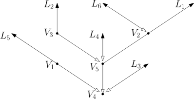
Figure 1: Stick breaking construction of a $\mathcal{D}$-tree with $\mathcal{D}=(1,2,1,3,3,0,0,\dots)$ and $(A^{\mathcal{D}}_{i})_{1\leq i\leq s-1}=(V_{4},V_{5},V_{2},V_{5},V_{3},V_{4},V_{5},V_{4},V_{1},V_{2})$. The exploration starts at $V_{4}$ then follows the white-black arrow toward $L_{1}$, then jumps at $V_{5}$ to follow the path toward $L_{2}$ and so on…

Proposition 1.

For every $\mathcal{D}\in\Omega_{\mathcal{D}}$, $T^{\mathcal{D}}$ is a $\mathcal{D}$-tree.

Proof.

See Appendix. ∎

Remarks.

(a) Addario-Berry, Donderwinkel, Maazoun, and Martin [28] independently found the same construction while I was writing the article.
(b) We introduce later a generalisation of Algorithm 1, Algorithm 6, which will be used to simplify many of our computations.
(c) One might prefer to consider "pure degree sequence": A tree $T$ is said have pure degree sequence $(d_{i})_{1\leq i\leq s}$ if $T$ have vertices $(V_{i})_{1\leq i\leq s}$, and for every $1\leq i\leq s$, $V_{i}$ have degree $d_{i}$ (not $d_{i}$ children). From a tree $T$ with pure degree sequence $(d_{1},\dots,d_{s})$ with $d_{s}=1$, one can construct a tree with degree sequence $(d_{1}-1,\dots,d_{s-1}-1)$ by rooting $T$ at the unique vertex adjacent to $V_{s}$ and then removing $V_{s}$. This is a well known bijection between tree with pure degree sequence $(d_{1},\dots,d_{s})$ and tree with degree sequence $(d_{1}-1,\dots,d_{s-1}-1)$. Since this bijection only removes one leaf, it does not change much the geometry of the tree. So our results on $\mathcal{D}$-trees easily adapt to uniform trees with fixed pure degree sequence.

As claimed in the introduction 1.2 (d), we are interested in the stick-breaking point of view to prove the convergence of $\mathcal{D}$-trees. To this end, let us formally define the cuts and the glue points. Note that there is $N:=\sum_{i=1}^{s}(d_{i}-1)\mathbf{1}_{d_{i}\geq 1}$ indexes $Y_{1}$, …$Y_{N}$ such that $A_{i}\in\{A_{1},\dots,A_{i-1}\}$. Also, for every $1\leq i\leq N$, let $Z_{i}$ denotes the smallest integer $z$ such that $A_{z}=A_{Y_{i}}$. We call $\{Y_{i}\}_{1\leq i\leq N}$ the cuts, and $\{Z_{i}\}_{1\leq i\leq N}$ the glue points.

Let us introduce some new tools to study those processes. First, note that the cuts and the glue points are encoded by "when" and "where" there are some "repetitions" in $A^{\mathcal{D}}$. Therefore, it is natural to look at the law of $A_{i}$ conditioned on $(A_{j})_{1\leq j<i}$. In particular, since $A^{\mathcal{D}}$ is a uniform $\mathcal{D}$-tuple, note that for every $1\leq i\leq s-1$ and $1\leq a\leq s$:

$$\mathbb{P}(A_{i}=V_{a}|(A_{j})_{1\leq j<i})=\frac{d_{a}-\#\{1\leq j<i:A_{j}=V_{a}\}}{s-i}.$$ (1)

Hence, we have for every $j<i\leq s-1$,

$$\mathbb{P}\left(\left.(i,j)\in\{(Y_{l},Z_{l})\}_{l\in\mathbb{N}}\right|(A_{k})_{1\leq k<i}\right)=\mathbf{1}_{A_{j}\notin\{A_{k}\}_{1\leq k<j}}\frac{d_{A_{j}}-\#\{1\leq k<i:A_{k}=A_{j}\}}{s-i}.$$ (2)

To fully understand the behavior of the cuts and the glue points, let us rewrite (2). Since we are mostly interested in the first cuts, note that typically $\#\{1\leq k<i:A_{k}=A_{j}\}=1$ and so we have the following informal approximation

$$\mathbb{P}\left(\left.(i,j)\in\{(Y_{l},Z_{l})\}_{l\in\mathbb{N}}\right|(A_{k})_{1\leq k<i}\right)\approx\frac{\mu(j)}{s-i},$$ (3)

where $\mu$ is the real measure defined by

$$\mu:=\sum_{j=1}^{s-1}\delta_{j}\mathbf{1}_{A_{j}\notin\{A_{k}\}_{1\leq k<j}}\left(d_{A_{j}}-1\right).$$ (4)

As a result, the cuts and glue points are mostly encoded by this measure $\mu$. Finally to understand the behavior of $\mu$, let us rewrite (4). Let for every $i\in\mathbb{N}$,

$$X_{i}:=\inf\{1\leq j\leq s,A_{j}=V_{i}\}.$$

(by convention $X_{i}=\infty$ and $\delta_{\infty}=0$ when there is no such index) and note that

$$\mu=\sum_{i=1}^{s}\delta_{X_{i}}(d_{i}-1).$$ (5)

So $\mu$ can be directly studied through $(X_{i})_{1\leq i\leq s}$.

Finally we need to rescale $\mathcal{D}$-trees. So let for $\mathcal{D}\in\Omega_{\mathcal{D}}$, $(\sigma^{\mathcal{D}})^{2}:=\sum_{i=1}^{s}d_{i}(d_{i}-1)$.

2.2 $\mathcal{P}$-trees: construction and connection with $\mathcal{D}$-trees

Fix $({\mathcal{D}_{n}})_{n\in\mathbb{N}}$ a sequence in $\Omega_{\mathcal{D}}$ and assume that for every $i\in\mathbb{N}$, $d^{{\mathcal{D}_{n}}}_{i}/s^{{\mathcal{D}_{n}}}\to p_{i}$ as $n\to\infty$. Note that $p_{\infty}:=1-\sum_{i=1}^{\infty}p_{i}\geq 0$. We suppose further that $p_{1}>0$ and let $\mathcal{P}:=(p_{i})_{i\in\mathbb{N}\cup\{\infty\}}$.

In this regime $(A^{{\mathcal{D}_{n}}})_{n\in\mathbb{N}}$ converges: Let $V_{\infty}$ be an additional vertex and put a metric on $\{V_{i}\}_{i\in\mathbb{N}\cup\{\infty\}}$ such that $V_{i}\to V_{\infty}$ as $i\to\infty$. One can easily check that $(A^{{\mathcal{D}_{n}}})_{n\in\mathbb{N}}$ converges weakly toward $(A_{i}^{\mathcal{P}})_{i\in\mathbb{N}}$ as $n\to\infty$ where $(A_{i}^{\mathcal{P}})_{i\in\mathbb{N}}$ is a family of i.i.d. random variables such that for every $i\in\mathbb{N}\cup\{\infty\}$, $\mathbb{P}(A^{\mathcal{P}}_{1}=V_{i})=p_{i}$.

Hence, intuitively, the steps of Algorithm 1, which are encoded by those tuples, "converge". Therefore ${\mathcal{D}_{n}}$-trees should converge toward the tree $T^{\mathcal{P}}$ defined by the "limit algorithm":

Let $\Omega_{\mathcal{P}}$ be the set of sequence $(p_{i})_{i\in\mathbb{N}\cup\{\infty\}}$ in $\mathbb{R}^{+}$ such that $\sum_{i=1}^{\infty}p_{i}+p_{\infty}=1$, $p_{1}>0$ and $p_{1}\geq p_{2}\geq\dots$. For every $\mathcal{P}\in\Omega_{\mathcal{P}}$, the $\mathcal{P}$-tree is the tree constructed as follow:

Algorithm 2.

Definition of the $\mathcal{P}$-tree for $\mathcal{P}\in\Omega_{\mathcal{P}}$.

• Let $(A^{\mathcal{P}}_{i})_{i\in\mathbb{N}}$ be a family of i.i.d. random variables such that for all $i\in\mathbb{N}$, $\mathbb{P}(A^{\mathcal{P}}_{1}=V_{i})=p_{i}$.

• For every $i\in\mathbb{N}$, let $B^{\mathcal{P}}_{i}=A_{i}$ if $A_{i}\in\mathbb{N}$, and let $B^{\mathcal{P}}_{i}=V_{\infty,i}$ otherwise.

• Let $T^{\mathcal{P}}_{1}:=(\{B_{1}\},\emptyset)$ then for every $i\geq 2$ let

  $$T^{\mathcal{P}}_{i}:=\begin{cases}T_{i-1}\cup\{B_{i-1},B_{i}\}&\text{if }B_{i}\notin T_{i-1}.\\ T_{i-1}&\text{if }B_{i}\in T_{i-1}.\end{cases}$$ (6)

• Let $T^{\mathcal{P}}$ denotes the rooted tree $(\bigcup_{n\in\mathbb{N}}T_{n},B_{1})$.

Remarks.

(a) We choose to delete the leaves $\{L_{i}\}_{i\in\mathbb{N}}$ of $T^{\mathcal{P}}$ in (6) to avoid measurability issue.
(b) Note that the infinite vertex $V_{\infty}$ is split into many others. Indeed this vertex "fills the gap" produced by vertices with small degree. The introduction of $V_{\infty}$ allows us to consider a slightly more general definition than the one introduced in [19] which requires $\sum_{i=1}^{+\infty}p_{i}=1$.

Finally let us introduce a list of notations similar to those for $\mathcal{D}$-trees. For every $\mathcal{P}\in\Omega_{\mathcal{P}}$:

• Let $p_{1}^{\mathcal{P}},\dots,p_{\infty}^{\mathcal{P}}\in\mathbb{R}^{+}$ be such that $\mathcal{P}=(p_{1}^{\mathcal{P}},\dots,p_{\infty}^{\mathcal{P}})$.

• Let $s^{\mathcal{P}}:=\max\{i\in\mathbb{N}\cup\{\infty\},p_{i}>0\}$ and let $(\sigma^{\mathcal{P}})^{2}=\sum_{i=1}^{\infty}(p_{i})^{2}$.

• Let $(Y^{\mathcal{P}}_{i})_{i\in\mathbb{N}}$ be the indexes of repetitions in $(B_{i})_{i\in\mathbb{N}}$.

• For $i\in\mathbb{N}$, let $Z_{i}^{\mathcal{P}}:=\inf\{z,B_{z}=B_{Y_{i}}\}$.

• For $i\in\mathbb{N}$, let $X_{i}^{\mathcal{P}}=\inf\{j\in\mathbb{N},A_{j}=i\}$. Then let $\mu^{\mathcal{P}}=\sum_{i=1}^{\infty}p_{i}\delta_{X_{i}}$.

2.3 ICRT: construction and connection with $\mathcal{D}$-trees

Fix $({\mathcal{D}_{n}})_{n\in\mathbb{N}}\in\Omega_{\mathcal{D}}^{\mathbb{N}}$ and assume that $d_{1}^{\mathcal{D}_{n}}/s^{\mathcal{D}_{n}}\to\infty$ and that $\forall i\in\mathbb{N}$, $d^{{\mathcal{D}_{n}}}_{i}/\sigma^{{\mathcal{D}_{n}}}\to\theta_{i}$ as $n\to\infty$. Note that $\sum_{i=1}^{\infty}\theta_{i}^{2}\leq 1$ and let $\theta_{0}:=1-\sum_{i=1}^{\infty}\theta_{i}^{2}$. Then let $\Theta:=(\theta_{i})_{i\in\{0\}\cup\mathbb{N}}$.

Let us briefly explain why ${\mathcal{D}_{n}}$-trees converge in this regime. We stay informal here, and details are done in Section 5.3. First some quick estimates show that $(X^{\mathcal{D}_{n}}_{i}/\sigma^{\mathcal{D}_{n}})_{i\in\mathbb{N}}$ converge weakly toward some exponential random variables $(X_{i}^{\Theta})_{i\in\mathbb{N}}$. By (5), this implies that after proper rescaling $(\mu^{\mathcal{D}_{n}})_{n\in\mathbb{N}}$ should converges weakly toward some random measure $\mu^{\Theta}$. Finally, by (3) the cuts and the glue points are "encoded" by $\mu^{\mathcal{D}_{n}}$, so they should also converge after rescaling.

Those estimates suggest that ${\mathcal{D}_{n}}$-trees should converge after rescaling toward some limit tree. If one pursue the computation further, then one notice that this tree is in fact the $\Theta$-ICRT.

We now construct the $\Theta$-ICRT. First let us introduce a generic stick breaking construction. It takes for input two sequences in $\mathbb{R}^{+}$ called cuts ${\textbf{y}}=(y_{i})_{i\in\mathbb{N}}$ and glue points ${\textbf{z}}=(z_{i})_{i\in\mathbb{N}}$, which satisfy

$$\forall i<j,\ \ y_{i}<y_{j}\qquad;\qquad y_{i}\operatorname*{\longrightarrow}\infty\qquad;\qquad\forall i\in\mathbb{N},\ \ z_{i}\leq y_{i},$$

and creates an $\mathbb{R}$-tree (loopless geodesic metric space) by recursively "gluing" segment $(y_{i},y_{i+1}]$ on position $z_{i}$ (see Figure 5), or rigorously, by constructing a consistent sequence of distances $(d_{n})_{n\in\mathbb{N}}$ on $([0,y_{n}])_{n\in\mathbb{N}}$.

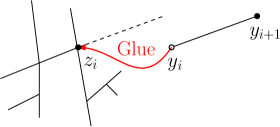
Figure 2: A typical step of the stick-breaking construction: the "gluing" of $(y_{i},y_{i+1}]$ at $z_{i}$.

Algorithm 3.

Generic stick-breaking construction of $\mathbb{R}$-tree.

• Let $d_{0}$ be the trivial metric on $[0,0]$.

• For each $i\geq 0$ define the metric $d_{i+1}$ on $[0,y_{i+1}]$ such that for each $x\leq y$:

  $$d_{i+1}(x,y):=\begin{cases}d_{i}(x,y)&\text{if }x,y\in[0,y_{i}]\\ d_{i}(x,z_{i})+|y-y_{i}|&\text{if }x\in[0,y_{i}],\,y\in(y_{i},y_{i+1}]\\ |x-y|&\text{if }x,y\in(y_{i},y_{i+1}],\end{cases}$$

  where by convention $y_{0}:=0$ and $z_{0}:=0$.

• Let $d$ be the unique metric on $\mathbb{R}^{+}$ which agrees with $d_{i}$ on $[0,y_{i}]$ for each $i\in\mathbb{N}$.

• Let $\operatorname*{SB}({\textbf{y}},{\textbf{z}})$ be the completion of $(\mathbb{R}^{+},d)$.

Now, let $\Omega_{\Theta}$ be the space of sequences $(\theta_{i})_{i\in\{0\}\cup\mathbb{N}}$ in $\mathbb{R}^{+}$ such that $\sum_{i=0}^{\infty}\theta_{i}^{2}=1$ and such that $\theta_{1}\geq\theta_{2}\geq\dots$. For every $\Theta\in\Omega_{\Theta}$, the $\Theta$-ICRT is the random $\mathbb{R}$-tree constructed as follow:

Algorithm 4.

Construction of $\Theta$-ICRT (from [12])

• Let $(X_{i})_{i\in\mathbb{N}}$ be a family of independent exponential random variables of parameter $(\theta_{i})_{i\in\mathbb{N}}$.

• Let $\mu$ be the measure on $\mathbb{R}^{+}$ defined by $\mu=\theta_{0}^{2}dx+\sum_{i=1}^{\infty}\delta_{X_{i}}\theta_{i}$.

• Let $(Y_{i},Z_{i})_{i\in\mathbb{N}}$ be a Poisson point process on $\{(y,z)\in\mathbb{R}^{+2}:y\geq z\}$ of intensity $dy\times d\mu$.

• The $\Theta$-ICRT is defined as $(\mathcal{T},d)=\operatorname*{SB}((Y_{i})_{i\in\mathbb{N}},(Z_{i})_{i\in\mathbb{N}})$. (see Algorithm 3)

Remarks.

(a) Although one usually excludes the ICRT with $\theta_{0}=0$ and $\sum_{i=1}^{\infty}\theta_{i}<\infty$, there are some $\mathcal{D}$-trees which converge toward such ICRT. Furthermore those ICRT may be seen as $\mathcal{P}$-trees with a modified distance (see section 5.2).
(b) The term $\theta_{0}^{2}dx$ in $\mu^{\theta}$ encompass the fact that some cuts may occur "because" of vertices with small degree. The case where $\theta_{0}=1$ corresponds to the Brownian CRT.

3 Notions of convergence

The reader may wish to simply skim this section on a first reading, referring back to it as needed.

3.1 Stick-breaking topology

Let $\mathbb{M}$ denotes the set of locally finite positive Borel measure on $\mathbb{R}^{+}$. Let $\mathbb{K}_{\text{SB}}:=(\mathbb{R}^{+})^{3\mathbb{N}}\times\mathbb{M}$. For every $\Lambda\in\Omega:=\Omega_{\mathcal{D}}\cup\Omega_{\mathcal{P}}\cup\Omega_{\Theta}$ let

$$\Upsilon^{\Lambda}:=((X_{i}^{\Lambda},Y_{i}^{\Lambda},Z_{i}^{\Lambda})_{i\in\mathbb{N}},\mu^{\Lambda})\in\mathbb{K}_{\text{SB}},$$

where by convention for $\mathcal{D}\in\Omega_{\mathcal{D}}$, and $i>N^{\mathcal{D}}$, $Y_{i}=Z_{i}=+\infty$.

We say that a sequence $(((X_{i}^{n},Y_{i}^{n},Z_{i}^{n})_{i\in\mathbb{N}},\mu^{n}))_{n\in\mathbb{N}}$ converges toward $((X_{i},Y_{i},Z_{i})_{i\in\mathbb{N}},\mu)$ for the stick-breaking (SB) topology if and only if

• For every $i\in\mathbb{N}$, $X_{i}^{n}\to X_{i}$, $Y_{i}^{n}\to Y_{i}$, $Z_{i}^{n}\to Z_{i}$.

• For every $i,j\in\mathbb{N}$ , $\mathbf{1}_{X_{i}^{n}=Z_{j}^{n}}\to\mathbf{1}_{X_{i}=Z_{j}}$.

• $\mu^{n}\to\mu$ for the Skorohod topology on $\mathbb{M}$ (that is $l\mapsto\mu^{n}[0,l]$ converges toward $l\mapsto\mu[0,l]$).

Note that the SB topology on $\mathbb{K}_{\text{SB}}$ is well defined and that $\mathbb{K}_{\text{SB}}$ equipped with the SB topology is a Polish space (separable complete metrisable space) as a product of Polish spaces.

Remark.

b) is here to "avoid fusion" between two branching points. Although (b) is not used in this paper, it is crucial for our study in [11]. The presence of $(X_{i})_{i\in\mathbb{N}}$ is also motivated by [11].

Finally let us introduce some notations to rescale our trees on $\mathbb{K}_{\text{SB}}$. For every $\lambda_{1},\lambda_{2}>0$, and $\mu\in\mathbb{M}$ let $(\lambda_{1},\lambda_{2})\mu\in\mathbb{M}$ such that for every Borel set $B$,

$$(\lambda_{1},\lambda_{2})\mu(B)=\lambda_{2}\mu\{\lambda_{1}x,x\in B\}.$$

For every $\lambda_{1},\lambda_{2}>0$ and $\Upsilon:=\{(X_{i},Y_{i},Z_{i})_{i\in\mathbb{N}},\mu\}\in\mathbb{K}_{\text{SB}}$ let

$$(\lambda_{1},\lambda_{2})\Upsilon:=((\lambda_{1}X_{i},\lambda_{1}Y_{i},\lambda_{1}Z_{i})_{i\in\mathbb{N}},(\lambda_{1},\lambda_{2})\mu).$$

Note that for every $\lambda_{1},\lambda_{2}>0$, the map $\Upsilon\mapsto(f,\lambda)\Upsilon$ is continuous and so measurable.

3.2 Gromov–Prokhorov (GP) topology

A measured metric space is a triple $(X,d,\mu)$ such that $(X,d)$ is a Polish space and $\mu$ is a Borel probability measure on $X$. Two such spaces $(X,d,\mu)$, $(X^{\prime},d^{\prime},\mu^{\prime})$ are called isometry-equivalent if and only if there exists an isometry $f:X\to X^{\prime}$ such that if $f_{\star}\mu$ is the image of $\mu$ by $f$ then $f_{\star}\mu=\mu^{\prime}$. Let $\mathbb{K}_{\text{GP}}$ be the set of isometry-equivalent classes of measured metric space. Given a measured metric space $(X,d,\mu)$, we write $[X,d,\mu]$ for the isometry-equivalence class of $(X,d,\mu)$ and frequently use the notation $X$ for either $(X,d,\mu)$ or $[X,d,\mu]$.

We now recall the definition of the Prokhorov’s distance. Consider a metric space $(X,d)$. For every $A\subset X$ and $\varepsilon>0$ let $A^{\varepsilon}:=\{x\in X,d(x,A)<\varepsilon\}$. Then given two (Borel) probability measures $\mu$, $\nu$ on $X$, the Prokhorov distance between $\mu$ and $\nu$ is defined by

$$d_{P}(\mu,\nu):=\inf\{\text{ $\varepsilon>0$: $\mu\{A\}\leq\nu\{A^{\varepsilon}\}$ and $\nu\{A\}\leq\mu\{A^{\varepsilon}\}$, for all Borel set $A\subset X$}\}.$$

The Gromov–Prokhorov (GP) distance is an extension of the Prokhorov’s distance: For every $(X,d,\mu),(X^{\prime},d^{\prime},\mu^{\prime})\in\mathbb{K}_{\text{GP}}$ the Gromov–Prokhorov distance between $X$ and $X^{\prime}$ is defined by

$$d_{\text{GP}}((X,d,\mu),(X^{\prime},d^{\prime},\mu^{\prime})):=\inf_{S,\phi,\phi^{\prime}}d_{P}(\phi_{\star}\mu,\phi^{\prime}_{\star}\mu^{\prime}),$$

where the infimum is taken over all metric spaces $S$ and isometric embeddings $\phi:X\to S$, $\phi^{\prime}:X^{\prime}\to S$. $d_{\text{GP}}$ is indeed a distance on $\mathbb{K}_{\text{GP}}$ and $(\mathbb{K}_{\text{GP}},d_{\text{GP}})$ is a Polish space (see e.g. [1]).

Remark.

For stick breaking construction a natural choice for $S$ is the completion of $(\mathbb{R}^{+\mathbb{N}},\|\|_{1})$ as one may simply use one direction for each branch (see Aldous [5] for more details).

We use another convenient characterization of the GP topology which relies on convergence of distance matrices: For every measured metric space $(X,d^{X},\mu^{X})$ let $(x_{i}^{X})_{i\in\mathbb{N}}$ be a sequence of i.i.d. random variables of common distribution $\mu^{X}$ and let $M^{X}:=(d^{X}(x_{i}^{X},x_{j}^{X}))_{(i,j)\in\mathbb{N}^{2}}$. We have the following result from [33],

Lemma 2.

Let $(X^{n})_{n\in\mathbb{N}}\in\mathbb{K}_{\text{GP}}^{\mathbb{N}}$ and let $X\in\mathbb{K}_{\text{GP}}$ then $X^{n}\operatorname*{\longrightarrow}^{\text{GP}}X$ as $n\to\infty$ if and only if $M^{X^{n}}$ converges in distribution toward $M^{X}$.

For convenience issue we use the following extension of Lemma 2.

Lemma 3.

Let $(X^{n})_{n\in\mathbb{N}}\in\mathbb{K}_{\text{GP}}^{\mathbb{N}}$ and let $X\in\mathbb{K}_{\text{GP}}$. Let $(y^{X}_{i})_{i\in\mathbb{N}}$ be a sequence of random variables on $X$ and let $N^{X}:=(d^{X}(y_{i}^{X},y_{j}^{X}))_{(i,j)\in\mathbb{N}^{2}}$. If

$$M^{X_{n}}\operatorname*{\longrightarrow}^{(d)}N^{X}\quad\text{and}\quad\frac{1}{n}\sum_{i=1}^{n}\delta_{y^{X}_{i}}\operatorname*{\longrightarrow}^{(d)}\mu^{X},$$

then $X^{n}\operatorname*{\longrightarrow}^{\text{GP}}X$ and thus $M^{X}$ and $N^{X}$ have the same distribution.

Proof.

Fix $k\leq m\in\mathbb{N}$. Let $(A_{1},\dots,A_{k})$ be a uniform tuple of $k$ different integers in $\{1,\dots,m\}$. Since $M^{X_{n}}\to^{(d)}N^{X}$, we have

$$\left(d^{X^{n}}\left(x_{i}^{X^{n}},x_{j}^{X^{n}}\right)\right)_{1\leq i,j\leq k}=^{(d)}\left(d^{X^{n}}\left(x_{A_{i}}^{X^{n}},x_{A_{j}}^{X^{n}}\right)\right)_{1\leq i,j\leq k}\operatorname*{\longrightarrow}^{(d)}\left(d^{X}\left(y_{A_{i}}^{X},y_{A_{j}}^{X}\right)\right)_{1\leq i,j\leq k}.$$

Now since as $m\to\infty$, $\frac{1}{m}\sum_{i=1}^{m}\delta_{y^{X}_{i}}\to\mu^{X}$, taking $m\to+\infty$ in the above equation yields

$$\left(d^{X^{n}}\left(x_{i}^{X^{n}},x_{j}^{X^{n}}\right)\right)_{1\leq i,j\leq k}\operatorname*{\longrightarrow}^{(d)}\left(d^{X}\left(x_{i}^{X},x_{j}^{X}\right)\right)_{1\leq i,j\leq k}.$$

Finally, since $k$ is arbitrary, Lemma 2 concludes the proof. ∎

3.3 Gromov–Hausdorff (GH) topology

Let $\mathbb{K}_{\text{GH}}$ be the set of isometry-equivalent classes of compact metric space. For every metric space $(X,d)$, we write $[X,d]$ for the isometry-equivalent class of (X,d), and frequently use the notation $X$ for either $(X,d)$ or $[X,d]$.

For every metric space $(X,d)$, the Hausdorff distance between $A,B\subset X$ is given by

$$d_{H}(A,B):=\inf\{\varepsilon>0,A\subset B^{\varepsilon},B\subset A^{\varepsilon}\}.$$

The Gromov–Hausdorff distance between $(X,d)$,$(X^{\prime},d^{\prime})\in\mathbb{K}_{\text{GH}}$ is given by

$$d_{\text{GH}}((X,d),(X^{\prime},d^{\prime})):=\inf_{S,\phi,\phi^{\prime}}\left(d_{H}(\phi(X),\phi^{\prime}(X^{\prime}))\right),$$

where the infimum is taken over all metric spaces $S$ and isometric embeddings $\phi:X\to S$, $\phi^{\prime}:X^{\prime}\to S$. $d_{\text{GH}}$ is indeed a distance on $\mathbb{K}_{\text{GH}}$ and $(\mathbb{K}_{\text{GH}},d_{\text{GH}})$ is a Polish space. (see e.g. [1])

3.4 Gromov–Hausdorff–Prokhorov (GHP) topology

Let $\mathbb{K}_{\text{GHP}}\subset\mathbb{K}_{\text{GP}}$ be the set of isometry-equivalent classes of compact measured metric space. The Gromov–Hausdorff–Prokhorov distance between $(X,d,\mu)$,$(X^{\prime},d^{\prime},\mu^{\prime})\in\mathbb{K}_{\text{GHP}}$ is given by

$$d_{\text{GHP}}((X,d,\mu),(X^{\prime},d^{\prime},\mu^{\prime})):=\inf_{S,\phi,\phi^{\prime}}\left(d_{P}(\phi_{\star}\mu,\phi^{\prime}_{\star}\mu^{\prime})+d_{H}(\phi(X),\phi^{\prime}(X^{\prime}))\right),$$

where the infimum is taken over all metric spaces $S$ and isometric embeddings $\phi:X\to S$, $\phi^{\prime}:X^{\prime}\to S$. $d_{\text{GHP}}$ is indeed a distance on $\mathbb{K}_{\text{GHP}}$ and $(\mathbb{K}_{\text{GHP}},d_{\text{GHP}})$ is a Polish space. (see [1])

Note that GHP convergence implies GP convergence, then that random variables GHP measurable are also GH measurable. For every $[X,d,p]\in\mathbb{K}_{\text{GHP}}$, let $[X,d]$ denote its natural projection on $\mathbb{K}_{\text{GH}}$. Note that GHP convergence implies GH convergence of the projections on $\mathbb{K}_{\text{GH}}$, then that the projection on $\mathbb{K}_{\text{GH}}$ is a measurable function. We will need the following statement.

Lemma 4.

Let $([X^{n},d^{n},p^{n}])_{n\in\mathbb{N}}$ and $[X,d,p]$ be GHP measurable random variables in $\mathbb{K}_{\text{GHP}}$. Assume that almost surely $[X,d,p]$ have full support. Assume that $([X^{n},d^{n},p^{n}])_{n\in\mathbb{N}}$ converges weakly toward $[X,d,p]$ in a GP sens, and that $([X^{n},d^{n}])_{n\in\mathbb{N}}$ converges weakly toward $[X,d]$ in a GH sens. Then $([X,d,p])_{n\in\mathbb{N}}$ converges weakly toward $[X,d,p]$ in a GHP sens.

Proof.

See Appendix ∎

3.5 Measurability

We briefly explain why $\mathcal{D}$-trees, $\mathcal{P}$-trees, and $\Theta$-ICRT are measurable for the SB, GP, and GHP topologies. First $\mathcal{D}$-trees are measurable as discrete random variables. Then, it is easy to prove from the definitions of $X,Y,Z,\mu$, that $\mathcal{P}$-trees and ICRT are SB measurable. Also, it is proved in [8, 19] that $\mathcal{P}$-trees and ICRT are GP measurable. Furthermore, $\mathcal{P}$-trees are GHP measurable, since we restrict to a finite discrete case.

The GHP measurability of compact $\Theta$-ICRT is harder to prove so let us give a sketch of proof. Let for every $l>0$, $\mu^{\Theta}_{l}$ be the restriction of $\mu^{\Theta}$ to $[0,l]$ and let $\mathcal{T}^{\Theta}_{l}:=([0,l],d^{\Theta},\mu^{\Theta}_{l}/\mu^{\Theta}[0,l])$. One can show that, for every $l>0$, $\mathcal{T}^{\Theta}_{l}$ is GHP measurable by proving the continuity of $\operatorname*{SB}$ (Algorithm 3) from $\mathbb{K}_{\text{SB}}$ to those subtrees. Then, by Theorems 3.1 and 3.3 of [12], almost surely $\{\mathcal{T}^{\Theta}_{l}\}_{l\in\mathbb{R}+}$ converges toward $\mathcal{T}^{\Theta}$ for the GHP topology so $\mathcal{T}^{\Theta}$ is GHP measurable.

4 Main results

In the whole section $({\mathcal{D}_{n}})_{n\in\mathbb{N}}$, $({\mathcal{P}_{n}})_{n\in\mathbb{N}}$, $({\Theta_{n}})_{n\in\mathbb{N}}$ are fixed sequences in $\Omega_{\mathcal{D}}$, $\Omega_{\mathcal{P}}$, $\Omega_{\Theta}$ respectively. Furthermore we always work under one of the following regimes:

Assumption 1 (${\mathcal{D}_{n}}\Rightarrow\mathcal{P}$).

For all $i\geq 1$, $d_{i}^{\mathcal{D}_{n}}/s^{\mathcal{D}_{n}}\to p^{\mathcal{P}}_{i}$ and $s^{\mathcal{D}_{n}}\to\infty$.

Assumption 2 (${\mathcal{D}_{n}}\Rightarrow\Theta$).

For all $i\geq 1$, $d_{i}^{\mathcal{D}_{n}}/\sigma^{\mathcal{D}_{n}}\to\theta^{\Theta}_{i}$ and $d_{1}^{\mathcal{D}_{n}}/s^{\mathcal{D}_{n}}\to 0$.

Assumption 3 (${\mathcal{P}_{n}}\Rightarrow\Theta$).

For all $i\geq 1$, $p_{i}^{\mathcal{P}_{n}}/\sigma^{\mathcal{P}_{n}}\to\theta^{\Theta}_{i}$ and $p_{1}^{\mathcal{P}_{n}}\to 0$.

Assumption 4 (${\Theta_{n}}\Rightarrow\Theta$).

For all $i\geq 1$, $\theta_{i}^{{\Theta_{n}}}\to\theta^{\Theta}_{i}$.

A few words on $\Rightarrow$.

In most of the paper $\Rightarrow$ is only used as a notation. However, one can put a topology on $\Omega:=\Omega_{\mathcal{D}}\cup\Omega_{\mathcal{P}}\cup\Omega_{\Theta}$ such that $\Rightarrow$ corresponds with the notion of convergence on $\Omega$. Let us briefly explain the main advantages of this approach (see Section 8.1 for more details).

First, one can check that $(\Omega,\Rightarrow)$ is a Polish space, so one can do probability on this space. Moreover, one can see our results as continuity results for the function which associate to a set of parameters a tree. Hence, our results can be used to study trees with random degree distributions.

Furthermore one can check that $\Omega_{\mathcal{D}}$ is dense, so our results on $\mathcal{D}$-trees implies all the others.

4.1 Convergence of the first branches

Intuitively, the following technical result on Algorithms 1, 2, 4 tells that the first branches converge. It is absolutely central for this paper (recall Introduction 1.2) and also for the forthcoming [11].

Theorem 5.

The following convergences hold weakly for the SB topology (see Section 3.1).

• Suppose that ${\mathcal{D}_{n}}\Rightarrow\mathcal{P}$, then $(1,1/s^{\mathcal{D}_{n}})\Upsilon^{\mathcal{D}_{n}}\to^{\text{WSB}}\Upsilon^{\mathcal{P}}$.

• Suppose that ${\mathcal{D}_{n}}\Rightarrow\Theta$, then $(\sigma^{\mathcal{D}_{n}}/s^{\mathcal{D}_{n}},1/\sigma^{\mathcal{D}_{n}})\Upsilon^{\mathcal{D}_{n}}\to^{\text{WSB}}\Upsilon^{\Theta}$.

• Suppose that ${\mathcal{P}_{n}}\Rightarrow\Theta$, then $(\sigma^{\mathcal{P}_{n}},1/\sigma^{\mathcal{P}_{n}})\Upsilon^{\mathcal{P}_{n}}\to^{\text{WSB}}\Upsilon^{\Theta}.$

• Suppose that ${\Theta_{n}}\Rightarrow\Theta$, then $\Upsilon^{\Theta_{n}}\to^{\text{WSB}}\Upsilon^{\Theta}.$

4.2 Gromov–Prokhorov convergence

First let us specify the measures that we consider. Let $\Omega_{\mathfrak{p}}$ be the set of measures on $\{V_{i}\}_{i\in\mathbb{N}}$. We say that a sequence $(\mathfrak{p}_{n})_{n\in\mathbb{N}}\in\Omega_{\mathfrak{p}}^{\mathbb{N}}$ converges toward $\mathfrak{p}\in\Omega_{\mathfrak{p}}$ iff $\max_{i\in\mathbb{N}}|\mathfrak{p}_{n}(V_{i})-{\mathfrak{p}}(V_{i})|\to 0$. In the whole paper, for every $\mathcal{D}\in\Omega_{\mathcal{D}}$, $\mathfrak{p}^{\mathcal{D}}$ is a fixed probability measure with support on $\mathcal{V}^{\mathcal{D}}:=\{V_{i},1\leq i\leq s^{\mathcal{D}}\}$. Similarly, for every $\mathcal{P}\in\Omega_{\mathcal{P}}$, $\mathfrak{p}^{\mathcal{P}}$ is a fixed probability measure with support on $\mathcal{V}^{\mathcal{P}}:=\{V^{\mathcal{P}}_{i}\}_{i:p_{i}>0}$. Also, we sometimes let $0$ denotes the null measure on $\{V_{i}\}_{i\in\mathbb{N}}$.

Then we recall the probability measure on ICRT introduced in [12]. To simplify our expressions, we write $\mu^{\Theta}=\infty$ when either $\theta^{\Theta}_{0}>0$ or $\sum_{i=1}^{\infty}\theta^{\Theta}_{i}=\infty$, (since $\mu^{\Theta}=\infty$ iff a.s. $\mu^{\Theta}[0,\infty]=\infty$).

Definition ([12] Theorem 3.1).

Let $\Theta\in\Omega_{\Theta}$ be such that $\mu^{\Theta}=\infty$. For every $l>0$, let $\mu^{\Theta}_{l}$ be the restriction of $\mu^{\Theta}$ on $[0,l]$ and let ${\mathfrak{p}}^{\Theta}_{l}:=\mu^{\Theta}_{l}/\mu^{\Theta}[0,l]$. Almost surely there exists a probability measure ${\mathfrak{p}}^{\Theta}$ on $\mathcal{T}^{\Theta}$ such that $({\mathfrak{p}}^{\Theta}_{l})_{l>0}$ converges weakly toward ${\mathfrak{p}}^{\Theta}$.

Let us now state the main result of this section. In what follows, $d^{\mathcal{D}}$ denotes the graph distance on $T^{\mathcal{D}}$ and similarly $d^{\mathcal{P}}$ denotes the graph distance on $T^{\mathcal{P}}$.

Theorem 6.

The following convergences hold weakly for the GP topology (see Section 3.2).

• If ${\mathcal{D}_{n}}\Rightarrow\mathcal{P}$ and $\mathfrak{p}^{\mathcal{D}_{n}}\to\mathfrak{p}^{\mathcal{P}}$ then

  $$\left(\mathcal{V}^{\mathcal{D}_{n}},d^{\mathcal{D}_{n}},\mathfrak{p}^{\mathcal{D}_{n}}\right)\operatorname*{\longrightarrow}^{\text{WGP}}(\mathcal{V}^{\mathcal{P}},d^{\mathcal{P}},\mathfrak{p}^{\mathcal{P}}).$$

• If ${\mathcal{D}_{n}}\Rightarrow\Theta$, $\mathfrak{p}^{\mathcal{D}_{n}}\to 0$, and $\mu^{\Theta}=\infty$ then

  $$\left(\mathcal{V}^{\mathcal{D}_{n}},(\sigma^{\mathcal{D}_{n}}/s^{\mathcal{D}_{n}})d^{\mathcal{D}_{n}},\mathfrak{p}^{\mathcal{D}_{n}}\right)\operatorname*{\longrightarrow}^{\text{WGP}}(\mathcal{T}^{\Theta},d^{\Theta},{\mathfrak{p}}^{\Theta}).$$

• If ${\mathcal{P}_{n}}\Rightarrow\Theta$, $\mathfrak{p}^{\mathcal{P}_{n}}\to 0$, and $\mu^{\Theta}=\infty$ then

  $$\left(\mathcal{V}^{\mathcal{P}_{n}},\sigma^{\mathcal{P}_{n}}d^{\mathcal{P}_{n}},\mathfrak{p}^{\mathcal{P}_{n}}\right)\operatorname*{\longrightarrow}^{\text{WGP}}(\mathcal{T}^{\Theta},d^{\Theta},{\mathfrak{p}}^{\Theta}).$$

• If ${\Theta_{n}}\Rightarrow\Theta$, and $\mu^{\Theta}=\infty$ then

  $$(\mathcal{T}^{\Theta_{n}},d^{\Theta_{n}},{\mathfrak{p}}^{\Theta_{n}})\operatorname*{\longrightarrow}^{\text{WGP}}(\mathcal{T}^{\Theta},d^{\Theta},{\mathfrak{p}}^{\Theta}).$$

Remarks.

$\bullet$ Theorem 6 (a) follows from Theorem 5 (a) since we are considering discrete trees.
$\bullet$ There are several canonical measures on trees: uniform on leaves, uniform on vertices…We use generic measures $\mathfrak{p}^{\mathcal{D}_{n}}$ so that Theorem 6 applies to such a variety of measures.
$\bullet$ If $\mathfrak{p}^{\mathcal{D}_{n}}$ denotes the uniform measure on the leaves of $T^{{\mathcal{D}_{n}}}$, then Theorem 6 (b) mostly follows from Theorem 5 (b), Lemma 3 and the weak convergence $\frac{1}{n}\sum_{i=1}^{n}\delta_{Y^{\Theta}_{i}}\to{\mathfrak{p}}^{\Theta}$([12] Proposition 3.2). To prove the convergence for general $\mathfrak{p}^{\mathcal{D}_{n}}$ we use a coupling between Algorithms 1 and 6.
$\bullet$ In passing, by Lemma 3, we reprove (see [8] Theorem 9) that cut points "are" uniform vertices: Let $\Theta\in\Omega_{\Theta}$ such that $\mu^{\Theta}=\infty$. Let $(A^{\Theta}_{i})$ be a family of i.i.d.random variables with law $p^{\Theta}$. Then

$$(d^{\Theta}(Y_{i}^{\Theta},Y_{j}^{\Theta}))_{i,j\in\mathbb{N}}=^{(d)}(d^{\Theta}(A_{i}^{\Theta},A_{j}^{\Theta}))_{i,j\in\mathbb{N}}.$$

$\bullet$ Results (c) and (d) are already mostly proved by Aldous, Camarri and Pitman in [8, 19]. Our only contribution to those results is the small extension of the $\mathcal{P}$-tree model.

4.3 Gromov–Hausdorff–Prokhrov convergence

We deduce (see Lemma 4) the GHP convergence, from the GP convergence given by Theorem 6, and the GH convergence. To prove the GH convergence, we use the convergence of the first branches, and prove that the whole trees are close from their first branches. We already estimated the distance between the ICRT and its first branches in [12], and we apply similar methods for $\mathcal{D}$-trees and $\mathcal{P}$-trees. From those estimates, we know when there is convergence, and so state assumptions to focus only on those cases.

Let us enter the details. We proved in [12] Section 6 the following approximation for ICRT:

$$d_{H}(\mathcal{T}^{\Theta}_{y},\mathcal{T}^{\Theta})\approx\int_{y}^{\infty}\frac{dl}{l\mathbb{E}[\mu^{\Theta}[0,l]]},$$ (7)

where for every $\Theta\in\Omega_{\Theta}$ and $y\in\mathbb{R}^{+}$, $\mathcal{T}^{\Theta}_{y}=([0,y],d^{\Theta},{\mathfrak{p}}^{\Theta}_{y})$. Hence, since we want the trees to be close from their first branches, we assume for ICRT that:

Assumption 5.

$$\lim_{y\to+\infty}\limsup_{n\to+\infty}\int_{y}^{+\infty}\frac{dl}{l\mathbb{E}[\mu^{\Theta_{n}}[0,l]]}=0.$$

Let us make a similar assumption for $\mathcal{P}$-trees. Here, the previous integral does not converge since $\mu^{\mathcal{P}}[0,\infty]=\sum_{i=1}^{\infty}p_{i}<\infty$. To solve this issue, we truncate the integral and rely on from the following generalisation of (7):

$$d_{H}(\mathcal{T}^{\Theta}_{y},\mathcal{T}_{y^{\prime}}^{\Theta})\approx\int_{y}^{y^{\prime}}\frac{dl}{l\mathbb{E}[\mu^{\Theta}[0,l]]}.$$ (8)

The main idea is then to take $y^{\prime}$ as large as possible such that the approximation (8) stays "optimal" and then to estimate $d_{H}(\mathcal{T}_{y^{\prime}},\mathcal{T})$. For this reason we assume for $\mathcal{P}$-trees that:

Assumption 6.

The two following assumptions hold:

• For every $\mathcal{P}\in\Omega_{\mathcal{P}}$, let $t^{\mathcal{P}}:=\inf\left\{l\in\mathbb{N},\,\mathbb{E}[\mu^{\mathcal{P}}[0,l]]\geq 1/2\right\}$ and let $\bar{\mu}^{\mathcal{P}}:=(\sigma^{\mathcal{P}},1/\sigma^{\mathcal{P}})\mu^{\mathcal{P}}$ (see Section 3.1 for definition of rescaled measure). We have,

  $$\lim_{y\to+\infty}\limsup_{n\to+\infty}\int^{\sigma^{\mathcal{P}_{n}}t^{\mathcal{P}_{n}}}_{y}\frac{dl}{l\mathbb{E}\left[\bar{\mu}^{\mathcal{P}_{n}}[0,l]\right]}=0.$$

• $\ln s^{\mathcal{P}_{n}}=o\left(1/\sigma^{\mathcal{P}_{n}}\right)$.

For $\mathcal{D}$-trees, we make similar assumptions with another one for vertices of degree 1. Those vertices have the particularity of "not adding mass" to $\mu$ while "adding length" to $T^{\mathcal{D}}$. This is an issue, since intuitively, as the construction goes on, adding vertices normally increases $\mu$ which results into having smaller branches.

Assumption 7.

The three following assumptions hold :

• Let for every $\mathcal{D}\in\Omega_{\mathcal{D}}$, $t^{\mathcal{D}}:=\inf\left\{l\in\mathbb{N},\,\mathbb{E}[\mu^{\mathcal{D}}[0,l]]\geq N^{\mathcal{D}}/2\right\}$ and $\bar{\mu}^{\mathcal{D}}:=(\sigma^{\mathcal{D}}/s^{\mathcal{D}},1/\sigma^{\mathcal{D}})\mu^{\mathcal{D}}$. We have,

  $$\lim_{y\to+\infty}\limsup_{n\to+\infty}\int_{y}^{\frac{\sigma^{\mathcal{D}_{n}}}{s^{\mathcal{D}_{n}}}t^{\mathcal{D}_{n}}}\frac{dl}{l\mathbb{E}\left[\bar{\mu}^{\mathcal{D}_{n}}[0,l]\right]}=0.$$

• $\ln\left(s^{\mathcal{D}_{n}}_{\geq 2}\right)\frac{s^{\mathcal{D}_{n}}}{N^{\mathcal{D}_{n}}}=o\left(\frac{s^{\mathcal{D}_{n}}}{\sigma^{\mathcal{D}_{n}}}\right)$ where for every $\mathcal{D}\in\Omega_{\mathcal{D}}$, $s^{\mathcal{D}}_{\geq 2}:=\#\{i\in\mathbb{N},d_{i}^{\mathcal{D}}\geq 2\}$.

• $\frac{\ln(N^{\mathcal{D}_{n}})}{\ln\left(s^{\mathcal{D}_{n}}/s_{1}^{\mathcal{D}_{n}}\right)}=o\left(\frac{s^{\mathcal{D}_{n}}}{\sigma^{\mathcal{D}_{n}}}\right)$ where for every $\mathcal{D}\in\Omega_{\mathcal{D}}$, $s^{\mathcal{D}}_{1}:=\#\{i\in\mathbb{N},d_{i}^{\mathcal{D}}=1\}$.

Remarks.

We discuss here the necessity of the different assumptions for the GHP convergence.
$\bullet$ First (i) corresponds to the compactness of ICRT. Although we do not prove it, we are conviced that (i) is necessary as one can adapt the argument of section 6.3 of [12] to prove that there is no possible convergence otherwise. In applications $t^{\mathcal{D}}$ and $t^{\mathcal{P}}$ are hard to compute, however since the integral "grows slowly" one can often choose much more convenient bounds for the integral.
$\bullet$ Although natural, Assumptions 6 (ii) and 7 (ii) are not necessary as Lemma 22 is sub-optimal.
$\bullet$ Assumption 7 (iii) is optimal: The right hand side is the typical distance between two vertices. The left hand side is the typical size of the longest paths that are composed of vertices of degree 1. Hence when those paths are too long ${\mathcal{D}_{n}}$-trees can not converge.
$\bullet$ Although (ii) and (iii) of Assumption 7 look similar, they are not equivalent. However, we have the following implications: If (ii) holds and either $s_{1}^{\mathcal{D}_{n}}=O(s_{\geq 2}^{\mathcal{D}_{n}})$ or $N^{\mathcal{D}_{n}}=O(s_{\geq 2}^{\mathcal{D}_{n}})$, then (iii) holds. If (iii) holds and $s_{\geq 2}^{\mathcal{D}_{n}}=O(s_{1}^{\mathcal{D}_{n}})$ then (ii) holds.

Theorem 7.

The following convergences hold weakly for the GHP-topology.

• If ${\mathcal{D}_{n}}\Rightarrow\Theta$, $\mathfrak{p}^{\mathcal{D}_{n}}\to 0$, and Assumption 7 is satisfied then

  $$\left(\mathcal{V}^{\mathcal{D}_{n}},(\sigma^{\mathcal{D}_{n}}/s^{\mathcal{D}_{n}})d^{\mathcal{D}_{n}},\mathfrak{p}^{\mathcal{D}_{n}}\right)\operatorname*{\longrightarrow}^{\text{WGHP}}(\mathcal{T}^{\Theta},d^{\Theta},{\mathfrak{p}}^{\Theta}).$$

• If ${\mathcal{P}_{n}}\Rightarrow\Theta$, $\mathfrak{p}^{\mathcal{P}_{n}}\to 0$, and Assumption 6 is satisfied then

  $$\left(\mathcal{V}^{\mathcal{P}_{n}},\sigma^{\mathcal{P}_{n}}d^{\mathcal{P}_{n}},\mathfrak{p}^{\mathcal{P}_{n}}\right)\operatorname*{\longrightarrow}^{\text{WGHP}}(\mathcal{T}^{\Theta},d^{\Theta},{\mathfrak{p}}^{\Theta}).$$

• If ${\Theta_{n}}\Rightarrow\Theta$, and Assumption 5 is satisfied then

  $$(\mathcal{T}^{\Theta_{n}},d^{\Theta_{n}},{\mathfrak{p}}^{\Theta_{n}})\operatorname*{\longrightarrow}^{\text{WGHP}}(\mathcal{T}^{\Theta},d^{\Theta},{\mathfrak{p}}^{\Theta}).$$

Our proof of Theorem 7 follows a method of Aldous [5]. The main idea is to upper bound for a suitable sequence $(k_{n})$, the sum $\sum_{n}d_{H}(\mathcal{T}_{Y_{k_{n}}},\mathcal{T}_{Y_{k_{n+1}}})$. To this end note that for every $n$,

$$d_{H}(\mathcal{T}_{Y_{k_{n}}},\mathcal{T}_{Y_{k_{n+1}}})=\max_{k_{n}<i\leq k_{n+1}}d(Y_{i},\mathcal{T}_{Y_{k_{n}}}),$$

and that for $i>k_{n}$,

$$d(Y_{i},\mathcal{T}_{Y_{k_{n}}})=^{(d)}d(Y_{k_{n}+1},\mathcal{T}_{Y_{k_{n}}})=Y_{k_{n}+1}-Y_{k_{n}}.$$

The rest of the proof is just a computation using large deviation inequalities and union bounds.

Remark.

This method was used in [5] to prove that the Brownian CRT is compact, and by taking the limit of those bounds one can give an alternative proof for the compactness of ICRT.

4.4 Height of $\mathcal{D}$-trees, $\mathcal{P}$-trees and ICRT

With the same method, we obtain some upper bounds for the height of $\mathcal{D}$-trees, $\mathcal{P}$-trees and ICRT:

Theorem 8.

There exists some constants $c,C>0$ such that:

• For every $\mathcal{D}\in\Omega_{\mathcal{D}}$ and $x\in\mathbb{R}^{+}$:

  $$\mathbb{P}\left(c\frac{\sigma^{\mathcal{D}}}{s^{\mathcal{D}}}H(T^{\mathcal{D}})>x+\int_{1}^{\frac{\sigma^{\mathcal{D}}}{s^{\mathcal{D}}}t^{\mathcal{D}}}\frac{dl}{l\mathbb{E}[\bar{\mu}^{\mathcal{D}}[0,l]]}+\frac{\ln(s^{\mathcal{D}}_{\geq 2})\sigma^{\mathcal{D}}}{N^{\mathcal{D}}}+\frac{\sigma^{\mathcal{D}}}{s^{\mathcal{D}}}\frac{\ln(N^{\mathcal{D}})}{\ln\left(\frac{s^{\mathcal{D}}}{s_{1}^{\mathcal{D}}}\right)}\right)\leq Ce^{-cx\mathbb{E}[\bar{\mu}^{\mathcal{D}}[0,x]]}.$$

• For every $\mathcal{P}\in\Omega_{\mathcal{P}}$ and $x\in\mathbb{R}^{+}$:

  $$\mathbb{P}\left(c\sigma^{\mathcal{P}}H(T^{\mathcal{P}})>x+\int_{1}^{\sigma^{\mathcal{P}}t^{\mathcal{P}}}\frac{dl}{l\mathbb{E}[\bar{\mu}^{\mathcal{P}}[0,l]]}+\sigma^{\mathcal{P}}\ln(s^{\mathcal{P}})\right)\leq Ce^{-cx\mathbb{E}[\bar{\mu}^{\mathcal{P}}[0,x]]}.$$

• For every $\Theta\in\Omega_{\Theta}$ and $x\in\mathbb{R}^{+}$:

  $$\mathbb{P}\left(cH(\mathcal{T}^{\Theta})>x+\int_{x}^{+\infty}\frac{dl}{l\mathbb{E}[\mu^{\Theta}[0,l]]}\right)\leq Ce^{-cx\mathbb{E}[\mu^{\Theta}[0,x]]}.$$

Remarks.

$\bullet$ There is a (non matching) lower bound in the case of the ICRT. Indeed, note that $H(\mathcal{T}^{\Theta})\geq Y_{1}^{\Theta}$ then that

$$\mathbb{P}(Y_{1}^{\Theta}\geq x|\mu^{\Theta})=e^{-\int_{0}^{x}\mu^{\Theta}[0,l]dl}\geq e^{-x\mu^{\Theta}[0,x]},$$

and then by convexity of $l\mapsto e^{l}$,

$$\mathbb{P}(Y_{1}^{\Theta}\geq x)\geq e^{-x\mathbb{E}[\mu^{\Theta}[0,x]]}.$$

Although we do not pursue in this direction, one can show similar bounds for $\mathcal{D}$-trees and $\mathcal{P}$-trees.
$\bullet$ The other terms are almost optimal as they correspond to Assumptions 5, 6, 7.
$\bullet$ Addario–Berry, Devroye, Janson [2] and Kortchemski [26] prove similar upper bounds for Galton–Watson trees and Lévy trees. Also Addario–Berry [3] prove a weaker result on $\mathcal{D}$-trees, which is similar to our result in the "small"-degree case and simpler to compute.

5 Convergence of the first branches of $\mathcal{D}$-trees

5.1 Convergence of $\mathcal{D}$-trees toward $\mathcal{P}$-trees: proof of Theorem 5 (a)

Recall Algorithms 1 and 2. Let $({\mathcal{D}_{n}})_{n\in\mathbb{N}}$ be a sequence in $\Omega_{\mathcal{D}}$ and let $\mathcal{P}\in\Omega_{\mathcal{P}}$ such that ${\mathcal{D}_{n}}\Rightarrow\mathcal{P}$. We saw in Section 2.2 that in this case $(A^{\mathcal{D}_{n}})_{n\in\mathbb{N}}$ converges weakly toward $A^{\mathcal{P}}$ as $n\to\infty$. Hence, we may assume that a.s. for every $i\in\mathbb{N}$, $A_{i}^{\mathcal{D}_{n}}\to A_{i}^{\mathcal{P}}$.

Our goal is to prove that $(1,1/s^{\mathcal{D}_{n}})\Upsilon^{\mathcal{D}_{n}}\to\Upsilon^{\mathcal{P}}$ for the SB topology defined in Section 3.1. Since we work with discrete random variables, note that it suffices to show that for every $i\in\mathbb{N}$, $X_{i}^{\mathcal{D}_{n}}\to X_{i}^{\mathcal{P}}$, $Y_{i}^{\mathcal{D}_{n}}\to Y_{i}^{\mathcal{P}}$, $Z_{i}^{\mathcal{D}_{n}}\to Z_{i}^{\mathcal{P}}$ and that $\mu^{\mathcal{D}_{n}}/s^{\mathcal{D}_{n}}\to\mu^{\mathcal{P}}$. First we have for every $i\in\mathbb{N}$,

$$X^{\mathcal{D}_{n}}_{i}=\inf\{j\in\mathbb{N},A^{\mathcal{D}_{n}}_{j}=V_{i}\}\operatorname*{\longrightarrow}\inf\{j\in\mathbb{N},A^{\mathcal{P}}_{j}=V_{i}\}=X_{i}^{\mathcal{P}}.$$

Then we have for the Skorohod topology: (There is no issue involved with the sum of diracs here since all atoms lie at integer point.)

$$\frac{1}{s^{\mathcal{D}_{n}}}\mu^{\mathcal{D}_{n}}=\sum_{i=1}^{s^{\mathcal{D}_{n}}}\delta_{X^{\mathcal{D}_{n}}_{i}}\frac{d^{\mathcal{D}_{n}}_{i}-1}{s^{\mathcal{D}_{n}}}\operatorname*{\longrightarrow}^{\operatorname*{sko}}\sum_{i=1}^{\infty}\delta_{X^{\mathcal{P}}_{i}}p^{\mathcal{P}}_{i}=\mu^{\mathcal{P}}.$$

We now study the cuts and the glue points which correspond to repetitions in $(A^{\mathcal{D}_{n}}_{i})_{1\leq i\leq s^{{\mathcal{D}_{n}}-1}}$. Here, some extra care is required since the vertex $V_{\infty}$ "is split" into many others in Algorithm 2. For every $i,j,k,n\in\mathbb{N}$, we have

$$\mathbb{P}\left(A^{\mathcal{D}_{n}}_{i}=A^{\mathcal{D}_{n}}_{j}\in\{V_{a}\}_{a>k}\right)=\sum_{a=k+1}^{+\infty}\frac{d^{\mathcal{D}_{n}}_{a}}{(s^{\mathcal{D}_{n}}-1)}\frac{(d^{\mathcal{D}_{n}}_{a}-1)}{(s^{\mathcal{D}_{n}}-2)}\leq\sum_{a=k+1}^{+\infty}\frac{1}{a^{2}}\operatorname*{\longrightarrow}_{k\to\infty}0.$$

So, we may also assume that for every $i,j\in\mathbb{N}$, there exists $k\in\mathbb{N}$ such that for every $n$ large enough we do not have $A^{\mathcal{D}_{n}}_{i}=A^{\mathcal{D}_{n}}_{j}\in\{V_{a}\}_{a>k}$. Or equivalently, for every $i,j\in\mathbb{N}$ such that $A_{i}^{\mathcal{P}}=A_{j}^{\mathcal{P}}=V_{\infty}$, for every $n$ large enough $A^{\mathcal{D}_{n}}_{i}\neq A^{\mathcal{D}_{n}}_{j}$. Also, for every $i,j\in\mathbb{N}$ such that $A_{i}^{\mathcal{P}}=A_{j}^{\mathcal{P}}\neq V_{\infty}$, for every $n$ large enough $A^{\mathcal{D}_{n}}_{i}=A^{\mathcal{D}_{n}}_{j}$. It directly follows that for every $i\in\mathbb{N}$, $Y_{i}^{\mathcal{D}_{n}}\to Y_{i}^{\mathcal{P}}$ and $Z_{i}^{\mathcal{D}_{n}}\to Z_{i}^{\mathcal{P}}$. This concludes the proof.

5.2 Preliminaries: $\mathcal{D}$-trees and $\mathcal{P}$-trees can be seen as modifications of ICRT

In this section, we give a rigorous meaning (Lemma 9) to the following informal statement: If one gives to each edge $e$ of a $\mathcal{P}$-tree a length $l_{e}$, such that $(l_{e})_{e\in T^{\mathcal{P}}}$ is a family of i.i.d. exponential random variables of mean $\sigma^{\mathcal{P}}$, then this $\mathcal{P}$-tree is quasi isometric to an ICRT. Also, although the connection between $\mathcal{D}$-trees and ICRT is not as simple, we prove a similar statement for $\mathcal{D}$-trees (Lemma 10), which is key in our proof of Theorem 5 (b).

First let us introduce "length change" on $\mathbb{K}^{\text{SB}}$ (recall Section 3.1). Let $\mathbb{F}$ be the set of increasing bijection from $\mathbb{R}^{+}$ to $\mathbb{R}^{+}$. For every $f\in\mathbb{F}$, $\lambda>0$ and $\Upsilon=((X_{i},Y_{i},Z_{i})_{i\in\mathbb{N}},\mu)\in\mathbb{K}_{\text{SB}}$, let

$$(f,\lambda)\Upsilon:=((f(X_{i}),f(Y_{i}),f(Z_{i}))_{i\in\mathbb{N}},\lambda f_{\star}\mu).$$

Note that for every $f\in\mathbb{F}$, $\lambda>0$, the map $\Upsilon\mapsto(f,\lambda)\Upsilon$ is continuous and so measurable.

Lemma 9.

Let $\mathcal{P}\in\Omega_{\mathcal{P}}$, let $\Theta=(0,p_{1}/\sigma,p_{2}/\sigma,\dots)$. Note that $\Theta\in\Omega_{\Theta}$. Let $\{l_{i}\}_{i\in\mathbb{N}}$ be a family of i.i.d. exponential random variables of mean $\sigma$. Let $f\in\mathbb{F}$ be such that for every $i\geq 0$, $f(\sigma i)=\sum_{k=1}^{i}l_{k}$. Then $(f,1/\sigma)\Upsilon^{\mathcal{P}}$ and $\Upsilon^{\Theta}$ have the same distribution.

Proof.

We omit the proof of Lemma 9 since it would be too similar to the proof of Lemma 10. (See also Camarri, Pitman [19] Section 4.1 who introduce a similar connection.) ∎

The connection between $\mathcal{D}$-trees and ICRT is not as simple. However we have the following construction which "replaces" ICRT.

Algorithm 5.

Definition of "the continuum $\mathcal{D}$-tree": $\tilde{\Upsilon}^{\mathcal{D}}$.

• Let $(\tilde{X}_{i})_{i\in\mathbb{N}}$ be a family of independent exponential random variables of parameter $(d_{i}/\sigma)_{i\in\mathbb{N}}$.

• Let $\tilde{\mu}$ be the measure on $\mathbb{R}^{+}$ defined by $\tilde{\mu}=\sum_{i=1}^{s}\delta_{\tilde{X}_{i}}\left(d_{i}-1\right)/\sigma$.

• Let $(\hat{Y}_{i},\hat{Z}_{i})_{i\in\mathbb{N}}$ be a Poisson point process on $\{(y,z)\in\mathbb{R}^{+2}:y\geq z\}$ of intensity $dy\times d\tilde{\mu}$.

• For every $i\in\mathbb{N}$ with $d_{i}\geq 1$, let $U_{X,i}$ be uniform in $\{1,\dots,d_{i}\}$.

• For every $j\in\mathbb{N}$, let $U_{j}$ be a uniform in $\{1,\dots,d_{i}\}\backslash\{U_{X,i}\}$ where $i$ is the unique index such that $\tilde{X}_{i}=\hat{Z}_{j}$. ($U_{j}$ is well defined since $\hat{Z}_{j}$ is in the support of $\tilde{\mu}$, which is $\{\tilde{X}_{i}\}_{i:d_{i}>0}$.)

• Let $k_{1}<\dots<k_{N}$ be the indexes such that $(Z_{k},U_{k})\notin\{(Z_{j},U_{j}),j<k\}$. (There is a.s. $N$ such indexes since $N=\sum_{i:d_{i}>0}d_{i}-1=\#\{(i,u)\in\mathbb{N}^{2}:\,d_{i}>0,1\leq u\leq d_{i},u\neq U_{X,i}\}$.)

• For every $1\leq i\leq N$, let $\tilde{Y}_{i}=\bar{Y}_{k_{i}}$ and let $\tilde{Z}_{i}=\bar{Z}_{k_{i}}$. For every $i>N$, let $\tilde{Y}_{i}=\tilde{Z}_{i}=+\infty$.

• Let $\tilde{\Upsilon}^{\mathcal{D}}=((\tilde{X}_{i},\tilde{Y}_{i},\tilde{Z}_{i})_{i\in\mathbb{N}},\tilde{\mu})$.

The following result is the analog of Lemma 9 for $\mathcal{D}$-trees.

Lemma 10.

Let $\mathcal{D}\in\Omega_{\mathcal{D}}$. Let $(E^{\mathcal{D}}_{i})_{1\leq i\leq s^{\mathcal{D}}-1}$ be a family of independent exponential random variables of mean $(\sigma^{\mathcal{D}}/(s^{\mathcal{D}}-i))_{1\leq i\leq s^{\mathcal{D}}-1}$ and let $f^{\mathcal{D}}\in\mathbb{F}$ such that for every $1\leq i\leq s^{\mathcal{D}}-1$, $f^{\mathcal{D}}(i)=\sum_{k=1}^{i}E^{\mathcal{D}}_{k}$. Then $(f^{\mathcal{D}},1/\sigma^{\mathcal{D}})\Upsilon^{\mathcal{D}}$ and $\tilde{\Upsilon}^{\mathcal{D}}$ have the same distribution.

Proof.

Note that it suffices to construct a coupling between Algorithms 1 and 5 such that a.s. $(f(X_{i}),f(Y_{i}),f(Z_{i}))_{i\in\mathbb{N}}=(\tilde{X}_{i},\tilde{Y}_{i},\tilde{Z}_{i})_{i\in\mathbb{N}}$. To this end we use the same "starting randomness" for both algorithms:

First let $I:=\{(i,j)\in\mathbb{N}^{2},1\leq i\leq s,1\leq j\leq d_{i}\}.$ For every $(i,j)\in I$, let $P_{i,j}$ be a Poisson point process on $\mathbb{R}^{+}$ with rate $1/\sigma$ and let $E_{i,j}=\min P_{i,j}$. For every $i\in\mathbb{N}$ such that $d_{i}\geq 1$ let $k_{i}=\operatorname*{argmin}\{E_{i,j},1\leq j\leq d_{i}\}$. Finally let $I_{2}=I\backslash\{i,k_{i}\}_{1\leq i\leq s}$.

Toward Algorithm 1, sort $\{(E_{i,j},V_{i},j)\}_{(i,j)\in I}$ by the first coordinate as $(t_{i},B_{i},K_{i})_{1\leq i\leq s-1}$. One can easily check, that $(t_{i})_{1\leq i\leq s-1}$ is independent of $(B_{i},k_{i})_{1\leq i\leq s-1}$, that $(t_{i})_{i\in\mathbb{N}}$ have the same distribution as $(f(i))_{1\leq i\leq s-1}$, and that $(B_{i},k_{i})_{1\leq i\leq s-1}$ is a uniform permutation of $I$. We omit the trivial details. As a result, $(t_{i},B_{i})_{1\leq i\leq s-1}$ have the same distribution as $(f(i),A_{i})_{1\leq i\leq s-1}$. Therefore we may assume that for every $1\leq i\leq s-1$, $(t_{i},B_{i})=(f(i),A_{i})$. It directly follows that for every $i\in\mathbb{N}$ such that $d_{i}\geq 1$,

$$f(X_{i})=f(\min\{j\in\mathbb{N},A_{j}=V_{i}\})=\min\{f(j),A_{j}=V_{i}\}=\min\{E_{i,k},1\leq k\leq d_{i}\}=E_{i,k_{i}}.$$ (9)

Then by a similar argument,

$$\{f(Y_{i}),f(Z_{i})\}_{1\leq i\leq N}=\{E_{i,j},E_{i,k_{i}}\}_{(i,j)\in I_{2}}.$$ (10)

Toward Algorithm 5, note that $E_{i,k_{i}}$ is an exponential random variable of mean $d_{i}/\sigma$ and that $k_{i}$ is uniform in $\{1,\dots,d_{i}\}$, hence we may assume that

$$\tilde{X}_{i}=E_{i,k_{i}}\quad;\quad U_{X,i}=k_{i}.$$ (11)

Then, note that conditionally on $(k_{i})_{1\leq i\leq s}$ and on $(E_{i,k_{i}})_{1\leq i\leq s}$, $\bigcup_{(i,j)\in I_{2}}P_{i,j}\times\{E_{i,k_{i}}\}\times\{j\}$ is a Poisson point process on $\mathbb{R}^{+3}$ of intensity

$$\sum_{(i,j)\in I_{2}}\mathbf{1}_{E_{i,k_{i}}\leq x}dx\times\delta_{E_{i,k_{i}}}\times\delta_{j}.$$ (12)

Also note that conditionally on $(\tilde{X}_{i})_{1\leq i\leq s}$ and on $(U_{X,i})_{1\leq i\leq s}$, $\{\hat{Y}_{i},\hat{Z}_{i},U_{Z,i}\}_{i\in\mathbb{N}}$ is also a Poisson point process with the same intensity as in (12). So we may assume that

$$\{\hat{Y}_{i},\hat{Z}_{i},U_{Z,i}\}_{i\in\mathbb{N}}=\bigcup_{(i,j)\in I_{2}}P_{i,j}\times\{E_{i,k_{i}}\}\times\{j\}.$$ (13)

Therefore, by "keeping" the first point of each line $\{y,z,u\}_{y\in\mathbb{R}^{+}}$ in both side and by "deleting" the last coordinate, we have,

$$\{\tilde{Y}_{i},\tilde{Z}_{i}\}_{1\leq i\leq N}=\{E_{i,j},E_{i,k_{i}}\}_{(i,j)\in I_{2}}.$$ (14)

Finally by (9) and (11) we have $(f(X_{i}))_{i\in\mathbb{N}}=(\tilde{X}_{i})_{i\in\mathbb{N}}$. Also by (10), (14), and by monotony of $(Y_{i})_{i\in\mathbb{N}}$ and $(\tilde{Y}_{i})_{i\in\mathbb{N}}$ we have $(f(Y_{i}),f(Z_{i}))_{i\in\mathbb{N}}=(\tilde{Y}_{i},\tilde{Z}_{i})_{i\in\mathbb{N}}$.∎

5.3 Convergence of $\mathcal{D}$-trees toward ICRT: proof of Theorem 5 (b)

Fix $({\mathcal{D}_{n}})_{n\in\mathbb{N}}\in\Omega_{\mathcal{D}}^{\mathbb{N}}$ and $\Theta\in\Omega_{\Theta}$. We assume that $\mathcal{D}_{n}\Rightarrow\Theta$, that is $d_{1}^{\mathcal{D}_{n}}/s^{\mathcal{D}_{n}}\to 0$ and $\forall i\in\mathbb{N}$, $d_{i}^{\mathcal{D}_{n}}/\sigma^{\mathcal{D}_{n}}\to\theta^{\Theta}_{i}$, and we prove that $(\sigma^{\mathcal{D}_{n}}/s^{\mathcal{D}_{n}},1/\sigma^{\mathcal{D}_{n}})\Upsilon^{\mathcal{D}_{n}}\to\Upsilon^{\Theta}$ weakly for the SB topology. To this end, we follow the steps of Algorithm 5 and concludes by using Lemma 10.

Lemma 11.

If ${\mathcal{D}_{n}}\Rightarrow\Theta$ then jointly in distribution for every $i\in\mathbb{N}$, $\tilde{X}^{\mathcal{D}_{n}}_{i}\to X^{\Theta}_{i}$ and $\tilde{\mu}^{\mathcal{D}_{n}}\to\mu$.

Proof.

The convergence of the variables $(\tilde{X}_{i}^{\mathcal{D}_{n}})_{i\in\mathbb{N}}$ is immediate from their definitions. Hence by the Skorohod representation theorem we may assume that almost surely for every $i\in\mathbb{N}$, $\tilde{X}^{\mathcal{D}_{n}}_{i}\operatorname*{\longrightarrow}X^{\Theta}_{i}$.

We now prove that jointly with the previous convergence, $\tilde{\mu}^{\mathcal{D}_{n}}\to\mu^{\Theta}$ weakly for the Skorohod topology. To this end, for every $\mathcal{D}\in\Omega_{\mathcal{D}}$ and $k\in\mathbb{N}$ we split $x\mapsto\tilde{\mu}^{\mathcal{D}}[0,x]$ into

$$F^{\mathcal{D},\leq k}:x\mapsto\sum_{i=1}^{k}\mathbf{1}_{\tilde{X}^{\mathcal{D}}_{i}\leq x}(d^{\mathcal{D}}_{i}-1)/\sigma^{\mathcal{D}}\quad\text{and}\quad F^{\mathcal{D},>k}:x\mapsto\sum_{i=k+1}^{\infty}\mathbf{1}_{\tilde{X}^{\mathcal{D}}_{i}\leq x}(d^{\mathcal{D}}_{i}-1)/\sigma^{\mathcal{D}}.$$

And we show that if $(k_{n})_{n\in\mathbb{N}}$ is a sequence increasing sufficiently slowly to $+\infty$ then for every $x>0$ (a) almost surely $F^{{\mathcal{D}_{n}},\leq k_{n}}(x)\to\sum_{i=1}^{\infty}\mathbf{1}_{X^{\Theta}_{i}\leq x}\theta_{i}$ and (b) $F^{{\mathcal{D}_{n}},>k_{n}}(x)\to\theta_{0}^{2}x$ in probability. Note that provided (c) $(\tilde{\mu}^{\mathcal{D}_{n}})^{n\in\mathbb{N}}$ is tight for the Skorohod topology, a sum of (a) and (b) yields the desired result.

Toward (a), recall that for every $i\in\mathbb{N}$, a.s. $\tilde{X}^{\mathcal{D}_{n}}_{i}\to X^{\Theta}_{i}$, and that ${\mathcal{D}_{n}}\Rightarrow\Theta$. So if $(k_{n})_{n\in\mathbb{N}}$ increases sufficiently slowly to $+\infty$ then by bounded convergence for every $x\in\mathbb{R}^{+}$ a.s.

$$F^{{\mathcal{D}_{n}},\leq k_{n}}(x)=\sum_{i=1}^{k_{n}}\mathbf{1}_{\tilde{X}^{\mathcal{D}_{n}}_{i}\leq x}(d^{\mathcal{D}_{n}}_{i}-1)/\sigma^{\mathcal{D}_{n}}\operatorname*{\longrightarrow}_{n\to\infty}\sum_{i=1}^{\infty}\mathbf{1}_{X^{\Theta}_{i}\leq x}\theta^{\Theta}_{i}.$$

To prove (b) we use a second moment method. We have for every $x\geq 0$,

$$\mathbb{E}\left[F^{{\mathcal{D}_{n}},>k_{n}}(x)\right]=\sum_{i=k_{n}+1}^{\infty}\frac{d^{\mathcal{D}_{n}}_{i}-1}{\sigma^{\mathcal{D}_{n}}}\mathbb{P}\left(\tilde{X}^{\mathcal{D}_{n}}_{i}\leq x\right)=\sum_{i=k_{n}+1}^{\infty}\frac{d^{\mathcal{D}_{n}}_{i}-1}{\sigma^{\mathcal{D}_{n}}}\left(1-\exp\left(x\frac{d^{\mathcal{D}_{n}}_{i}}{\sigma^{\mathcal{D}_{n}}}\right)\right).$$

Then, since $k_{n}\to\infty$ and since ${\mathcal{D}_{n}}\Rightarrow\Theta$,

$$\mathbb{E}\left[F^{{\mathcal{D}_{n}},>k_{n}}(x)\right]\sim\sum_{i=k_{n}+1}^{\infty}x\frac{d^{\mathcal{D}_{n}}_{i}-1}{\sigma^{\mathcal{D}_{n}}}\frac{d^{\mathcal{D}_{n}}_{i}}{\sigma^{\mathcal{D}_{n}}}=x-x\sum_{i=1}^{k_{n}}\frac{d_{i}^{\mathcal{D}_{n}}(d_{i}^{\mathcal{D}_{n}}-1)}{(\sigma^{\mathcal{D}_{n}})^{2}}\to x-x\sum_{i=1}^{+\infty}\theta_{i}^{2}=x\theta_{0}^{2},$$

where the last convergence holds by bounded convergence when $(k_{n})_{n\in\mathbb{N}}$ increases sufficiently slowly to $+\infty$. Also similarly for every $x\geq 0$,

$$\mathbb{V}\left[F^{{\mathcal{D}_{n}},>k_{n}}(x)\right]\leq\sum_{i=k_{n}+1}^{+\infty}\left(\frac{d^{\mathcal{D}_{n}}_{i}-1}{\sigma^{\mathcal{D}_{n}}}\right)^{2}\mathbb{P}\left(\tilde{X}^{\mathcal{D}_{n}}_{i}\leq x\right)\leq\frac{d^{\mathcal{D}_{n}}_{k_{n}+1}}{\sigma^{\mathcal{D}_{n}}}\mathbb{E}\left[F^{{\mathcal{D}_{n}},>k_{n}}(x)\right]=o(1).$$

And (b) follows.

Toward (c), for every $0\leq x\leq y\leq z$, and $n\in\mathbb{N}$ we have,

$$\Delta^{n}(x,y,z) :=\mathbb{E}\left[|\tilde{\mu}^{{\mathcal{D}_{n}}}(y)-\tilde{\mu}^{{\mathcal{D}_{n}}}(x)||\tilde{\mu}^{{\mathcal{D}_{n}}}(z)-\tilde{\mu}^{{\mathcal{D}_{n}}}(y)|\right]$$

$$=\mathbb{E}\left[\sum_{i=1}^{\infty}\mathbf{1}_{x<\tilde{X}^{\mathcal{D}_{n}}_{i}\leq y}\frac{d^{\mathcal{D}_{n}}_{i}-1}{\sigma^{\mathcal{D}_{n}}}\sum_{i=1}^{\infty}\mathbf{1}_{y<\tilde{X}^{\mathcal{D}_{n}}_{i}\leq z}\frac{d^{\mathcal{D}_{n}}_{i}-1}{\sigma^{\mathcal{D}_{n}}}\right]$$

$$=\sum_{i\neq j}\mathbb{P}\left(x<\tilde{X}^{\mathcal{D}_{n}}_{i}\leq y\right)\frac{d^{\mathcal{D}_{n}}_{i}-1}{\sigma^{\mathcal{D}_{n}}}\mathbb{P}\left(y<\tilde{X}^{\mathcal{D}_{n}}_{j}\leq z\right)\frac{d^{\mathcal{D}_{n}}_{j}-1}{\sigma^{\mathcal{D}_{n}}}$$

$$\leq\left(\sum_{i=1}^{\infty}\mathbb{P}\left(x<\tilde{X}^{\mathcal{D}_{n}}_{i}\leq z\right)\frac{d^{\mathcal{D}_{n}}_{i}-1}{\sigma^{\mathcal{D}_{n}}}\right)^{2}.$$ (15)

Then by definition of $(\tilde{X}_{i}^{\mathcal{D}_{n}})_{i\in\mathbb{N}}$ and by convexity of $x\mapsto e^{x}$,

$$\mathbb{P}(x<\tilde{X}^{\mathcal{D}_{n}}_{i}\leq z)=e^{-d_{i}^{\mathcal{D}_{n}}/\sigma^{\mathcal{D}_{n}}z}-e^{-d_{i}^{\mathcal{D}_{n}}/\sigma^{\mathcal{D}_{n}}x}\leq d_{i}^{\mathcal{D}_{n}}/\sigma^{\mathcal{D}_{n}}(z-x).$$

Hence, by (15) and definition of $\sigma^{\mathcal{D}_{n}}$,

$$\Delta^{n}(x,y,z)\leq\left(\sum_{i,\theta_{i}=1}^{\infty}\frac{d_{i}^{\mathcal{D}_{n}}}{\sigma^{\mathcal{D}_{n}}}(z-x)\frac{d^{\mathcal{D}_{n}}_{i}-1}{\sigma^{\mathcal{D}_{n}}}\right)^{2}=(z-x)^{2}.$$

Finally since $x,y,z$ are arbitrary (c) follows. ∎

It directly follows from Lemma 11, and the definition of $(\hat{Y}_{i}^{\mathcal{D}_{n}},\hat{Z}_{i}^{\mathcal{D}_{n}})$ (see Algorithm 5), that

$$\hat{\Upsilon}^{\mathcal{D}_{n}}:=((\tilde{X}_{i}^{\mathcal{D}_{n}},\hat{Y}_{i}^{\mathcal{D}_{n}},\hat{Z}_{i}^{\mathcal{D}_{n}})_{i\in\mathbb{N}},\tilde{\mu}^{\mathcal{D}})\operatorname*{\longrightarrow}^{\text{WSB}}_{n\to\infty}\Upsilon^{\Theta}.$$ (16)

We omit the trivial details, and refer for instance to Lemma 4.24 (ii’) of Kallenberg [25] for more precision on convergence of Poisson point process.

The following lemma implies that we can "replace" in (16) $(\hat{Y}_{i}^{\mathcal{D}_{n}},\hat{Z}_{i}^{\mathcal{D}_{n}})_{i\in\mathbb{N}}$ by $(\tilde{Y}_{i}^{\mathcal{D}_{n}},\tilde{Z}_{i}^{\mathcal{D}_{n}})_{i\in\mathbb{N}}$.

Lemma 12.

Assume that ${\mathcal{D}_{n}}\Rightarrow\Theta$ then for every $i\in\mathbb{N}$,

$$\mathbb{P}\left(\hat{Y}^{\mathcal{D}_{n}}_{i}=\tilde{Y}^{\mathcal{D}_{n}}_{i}\text{ and }\hat{Z}^{\mathcal{D}_{n}}_{i}=\tilde{Z}^{\mathcal{D}_{n}}_{i}\right)\operatorname*{\longrightarrow}_{n\to\infty}1.$$

Proof.

Let for $\mathcal{D}\in\Omega_{\mathcal{D}}$, $m^{\mathcal{D}}:=\inf((\tilde{Y}^{\mathcal{D}}_{i})_{i\in\mathbb{N}}\backslash(\hat{Y}^{\mathcal{D}}_{i})_{1\leq i\leq N})$. Note that it is enough to show that for every $l\in\mathbb{R}^{+}$, $\mathbb{P}(m^{\mathcal{D}_{n}}>l)\to 1$. To this end, we lower bound $\mathbb{P}(m^{\mathcal{D}}>l)$ for $\mathcal{D}$ and $l$ fixed.

First let us recall some notations introduced in the proof of Lemma 10. Let $I:=\{(i,j)\in\mathbb{N}^{2},1\leq i\leq s,1\leq j\leq d_{i}\}.$ For every $(i,j)\in I$, let $P_{i,j}$ be a Poisson point process on $\mathbb{R}^{+}$ with rate $1/\sigma$ and let $E_{i,j}=\min P_{i,j}$. For every $i$ such that $d_{i}\geq 1$ let $k_{i}=\operatorname*{argmin}\{E_{i,j},1\leq j\leq d_{i}\}$. Then let $I_{2}=I\backslash\{i,k_{i}\}_{1\leq i\leq s}$.

Now, recall that $\{\tilde{Y}_{i}\}_{i\in\mathbb{N}}\backslash\{\hat{Y}_{i}\}_{i\in\mathbb{N}}=\bigcup_{(i,j)\in I_{2}}\{P_{i,j}\backslash\{E_{i,j}\}\}$. So that by the union bound,

$$\mathbb{P}(m>l)\leq\sum_{i=1}^{s}\mathbb{P}\Big{(}\exists 1\leq j\leq d_{i}:(i,j)\in I_{2},\#(P_{i,j}\cap[0,l])\geq 2\Big{)}.$$ (17)

To simplify the notation, let $\sum_{1\leq i\leq s}S_{i}$ denote the sum above. We split this sum in two according to "whether $d_{i}$ is small or large", and we upper bound each part.

On the one hand, note that if there exists $1\leq j\leq d_{i}$ such that $(i,j)\in I_{2}$ and $\#(P_{i,j}\cap[0,l])\geq 2$ then $\#(\bigcup_{1\leq j\leq d_{i}}P_{i,j}\cap[0,l])\geq 3$ and $d_{i}\geq 2$. So that for every $1\leq i\leq s$,

$$S_{i}\leq\mathbb{P}\left(\#\left(\bigcup_{1\leq j\leq d_{i}}P_{i,j}\cap[0,l]\right)\geq 3\right)=1-e^{-ld_{i}/\sigma}\left(1+\frac{ld_{i}}{\sigma}+\frac{l^{2}d^{2}_{i}}{2\sigma^{2}}\right)\leq\left(l\frac{d_{i}}{\sigma}\right)^{3},$$

where the last inequality comes from the fact that for every $x\geq 0$, $1-e^{-x}(1+x+x^{2}/2)\leq x^{3}$. Then for every $\varepsilon>0$,

$$\sum_{i,d_{i}\leq\varepsilon\sigma}S_{i}\leq\sum_{i,d_{i}\leq\varepsilon\sigma}\mathbf{1}_{d_{i}\geq 2}\left(l\frac{d_{i}}{\sigma}\right)^{3}\leq 2l^{3}\varepsilon\sum_{i,d_{i}\leq\varepsilon\sigma}\frac{d_{i}(d_{i}-1)}{\sigma^{2}}\leq 2l^{3}\varepsilon.$$ (18)

On the other hand, we have by a similar argument,

$$S_{i}\leq d_{i}\mathbb{P}\left(\#(P_{i,1}\cap[0,l])\geq 2\right)\leq d_{i}l^{2}/\sigma^{2},$$

and when $\varepsilon\sigma>1$,

$$\sum_{i,d_{i}>\varepsilon\sigma}P_{i}\leq\sum_{i,d_{i}>\varepsilon\sigma}l^{2}\frac{d_{i}}{\sigma^{2}}\leq\sum_{i,d_{i}>\varepsilon\sigma}\frac{l^{2}}{\varepsilon\sigma-1}\frac{d_{i}(d_{i}-1)}{\sigma^{2}}\leq\frac{l^{2}}{\varepsilon\sigma-1}.$$ (19)

Therefore, summing (18) and (19), we have for every $n\in\mathbb{N}$,

$$\mathbb{P}(m^{\mathcal{D}_{n}}>l)\leq 2l^{3}\varepsilon+\frac{l^{2}}{\varepsilon\sigma^{\mathcal{D}_{n}}-1}.$$ (20)

Then as $n\to+\infty$, ${\mathcal{D}_{n}}\Rightarrow\Theta$ so $\sigma^{\mathcal{D}_{n}}\to\infty$ and the right hand term in (20) converges to $2\varepsilon$. Since $\varepsilon$ is arbitrary, $\mathbb{P}(m^{\mathcal{D}_{n}}>l)\to 0$. Since $l$ is arbitrary, this concludes the proof. ∎

Proof of Theorem 5 (b).

Recall for $\mathcal{D}\in\Omega_{\mathcal{D}}$ the definitions of $f^{\mathcal{D}}$ and $\{E_{i}^{\mathcal{D}}\}_{1\leq i<s^{\mathcal{D}}}$ introduced in Lemma 10. First it directly follows from Lemma 12 and equation (16) that weakly for the SB topology $\tilde{\Upsilon}^{\mathcal{D}_{n}}\to\Upsilon^{\Theta}$ as $n\to\infty$. Furthermore by Lemma 10, $(f^{\mathcal{D}_{n}},1/\sigma^{\mathcal{D}_{n}})\Upsilon^{\mathcal{D}_{n}}$ and $\tilde{\Upsilon}^{\mathcal{D}_{n}}$ have the same distribution. So, by Skorohod representation theorem we may assume that both the convergence and the equality holds almost surely, hence almost surely

$$(f^{\mathcal{D}_{n}},1/\sigma^{\mathcal{D}_{n}})\Upsilon^{\mathcal{D}_{n}}\to\Upsilon^{\Theta}.$$ (21)

Let for $n\in\mathbb{N}$, $\lambda_{n}:=s^{\mathcal{D}_{n}}/\sigma^{\mathcal{D}_{n}}$. For every $x\in\mathbb{R}^{+}$ and $n\in\mathbb{N}$, we have by definition of $f^{\mathcal{D}_{n}}$ and $\{E_{i}^{\mathcal{D}_{n}}\}_{1\leq i<s^{\mathcal{D}_{n}}}$,

$$\mathbb{E}\left[f^{\mathcal{D}_{n}}\left(\left\lfloor\lambda_{n}x\right\rfloor\right)\right]=\sum_{i=1}^{\lfloor\lambda_{n}x\rfloor}\mathbb{E}[E^{\mathcal{D}_{n}}_{i}]=\sum_{i=1}^{\lfloor\lambda_{n}x\rfloor}\frac{\sigma^{\mathcal{D}_{n}}}{s^{\mathcal{D}_{n}}-i}=\lfloor\lambda_{n}x\rfloor\frac{\sigma^{\mathcal{D}_{n}}}{s^{\mathcal{D}_{n}}-O(\lambda_{n})}\operatorname*{\longrightarrow}_{n\to\infty}x.$$

Similarly,

$$\mathbb{V}[f^{\mathcal{D}_{n}}(\lfloor\lambda_{n}x\rfloor)]=\sum_{i=1}^{\lfloor\lambda_{n}x\rfloor}\mathbb{V}[E_{i}]=\sum_{i=1}^{\lfloor\lambda_{n}x\rfloor}\left(\frac{\sigma^{\mathcal{D}}}{s^{\mathcal{D}}-i}\right)^{2}\operatorname*{\longrightarrow}0.$$

Therefore $x\mapsto f^{\mathcal{D}_{n}}(\lambda_{n}x)$ converges in distribution for $\|\cdot\|_{\infty}$ toward the identity on any interval. Then by Skorohod representation theorem we may assume that this convergence holds almost surely. The convergence $(1/\lambda_{n},1/\sigma^{\mathcal{D}_{n}})\Upsilon^{\mathcal{D}_{n}}\to^{\text{SB}}\Upsilon^{\Theta}$ then follows from (21) and a deterministic topological verification.∎

6 Gromov–Prokhorov convergence of $\mathcal{D}$-trees

6.1 Preliminary: vertices with small degree behaves like leaves

Recall that, by Lemma 3, to prove the GP convergence, it suffices to prove that the distance matrix between random vertices converges. To do so, we introduce a generalisation of Algorithm 1 which constructs sequentially the subtree spanned by the root and $W_{1},\dots,W_{i}$ where $W=\{W_{i}\}_{1\leq i\leq s^{\mathcal{D}}}$ is an arbitrary permutation of $\mathcal{V}^{\mathcal{D}}$. Then, we couple it with Algorithm 1 to show that whenever $W_{1},W_{2},\dots$ have "small" degree, then those subtrees are close from the subtrees spanned by the first leaves (see Lemma 14). This agrees with the intuition that vertices with small degree behave like leaves. Naturally, this is also true for random vertices, which typically are distinct and have small degree.

Algorithm 6.

General stick-breaking construction of $\mathcal{D}$-tree.

• Let $A^{\mathcal{D}}=(A_{1},\dots,A_{s-1})$ be a uniform $\mathcal{D}$-tuple.

• Let $T^{\mathcal{D},W}_{1}:=(\{A_{1}\},\emptyset)$ then for every $2\leq i\leq s$ let

  $$T^{\mathcal{D},W}_{i}:=\begin{cases}T_{i-1}\cup\{A_{i-1},A_{i}\}&\text{if }A_{i}\notin T_{i-1},\\ T_{i-1}\cup\{A_{i-1},W_{\inf\{k,W_{k}\notin T_{i-1}\}}\}&\text{if }A_{i}\in T_{i-1}\text{ or }i=s.\end{cases}$$

• Let $T^{\mathcal{D},W}$ denotes the rooted tree $(T_{s},A_{1})$.

Remark.

If for every $1\leq i\leq N+1$, $W_{i}=L_{i}$ then Algorithm 1 and Algorithm 6 follow the exact same steps, hence $T^{\mathcal{D},W}=T^{\mathcal{D}}$.

Proposition 13.

For every $\mathcal{D}\in\Omega_{\mathcal{D}}$, and $W$ permutation of $\mathcal{V}^{\mathcal{D}}$, $T^{\mathcal{D},W}$ is a $\mathcal{D}$-tree.

Proof.

See Appendix. ∎

Before stating the main result of this section, let us define the relabelling operation. For every graph $G=(V,E)$ and bijection $f:V\to V^{\prime}$, let $f(G):=(V^{\prime},\{\{f(x),f(y)\}\}_{\{x,y\}\in E})$.

Lemma 14.

Let $\mathcal{D}\in\Omega_{\mathcal{D}}$ and $W=\{W_{i}\}_{1\leq i\leq s^{\mathcal{D}}}$ be a permutation of $\mathcal{V}^{\mathcal{D}}$. Let $1\leq k\leq N^{\mathcal{D}}$ and let $f_{k}:\mathcal{V}^{\mathcal{D}}\to\mathcal{V}^{\mathcal{D}}$ be a bijection such that:

$$\forall 1\leq i\leq k\quad f_{k}(W_{i})=L_{i}\quad;\quad\forall V\notin\{W_{i}\}_{1\leq i\leq k}\cup\{L_{i}\}_{1\leq i\leq k}\quad f_{k}(V)=V.$$

Then for every $1\leq l\leq s^{\mathcal{D}}$, (where by convention for $i\in\mathbb{N}$, $d^{\mathcal{D}}_{V_{i}}:=d^{\mathcal{D}}_{i}$)

$$\mathbb{P}\left(f_{k}\left(T^{\mathcal{D},W}_{Y^{\mathcal{D}}_{k}}\right)\neq T^{\mathcal{D}}_{Y^{\mathcal{D}}_{k}}\right)\leq\mathbb{P}(Y^{\mathcal{D}}_{k}>l)+l\left(d^{\mathcal{D}}_{W_{1}}+\dots d^{\mathcal{D}}_{W_{k}}\right)/(s^{\mathcal{D}}-1).$$

Proof.

Note that $f_{k}(T^{W}_{Y_{k}})=T_{Y_{k}}$ whenever $\{W_{i}\}_{1\leq i\leq k}\cap\{A_{1},\dots,A_{Y_{k}}\}=\emptyset$, since in this case, up to relabelling, Algorithm 1 and Algorithm 6 follow the exact same steps. Therefore:

$$\mathbb{P}\left(f_{k}(T^{W}_{Y_{k}})\neq T_{Y_{k}}\right) \leq\mathbb{P}(Y_{k}>l)+\mathbb{P}(\{W_{i}\}_{1\leq i\leq k}\cap\{A_{1},\dots,A_{l}\}\neq\emptyset),$$

$$\leq\mathbb{P}(Y_{k}>l)+\sum_{i=1}^{l}\sum_{j=1}^{k}\mathbb{P}(A_{i}=W_{j}),$$

$$=\mathbb{P}(Y_{k}>l)+l\left(d_{W_{1}}+\dots d_{W_{k}}\right)/(s-1).\qed$$

6.2 Convergence of $\mathcal{D}$-trees toward ICRT: proof of Theorem 6 (b)

To simplify the notations we write for $\mathcal{D}\in\Omega_{\mathcal{D}}$, $\lambda^{\mathcal{D}}:=s^{\mathcal{D}}/\sigma^{\mathcal{D}}$.

First recall the assumptions of Theorem 6 (b): ${\mathcal{D}_{n}}\Rightarrow\Theta$, $\mathfrak{p}^{\mathcal{D}_{n}}\to 0$, and $\mu^{\Theta}=\infty$. In this case we have by Theorem 5 (b) the following joint convergence in distribution,

$$((Y_{i}^{\mathcal{D}_{n}}/\lambda^{\mathcal{D}_{n}})_{i\in\mathbb{N}},(Z_{i}^{\mathcal{D}_{n}}/\lambda^{\mathcal{D}_{n}})_{i\in\mathbb{N}})\operatorname*{\longrightarrow}^{\text{W}}((Y_{i}^{\Theta})_{i\in\mathbb{N}},(Z_{i}^{\Theta})_{i\in\mathbb{N}}).$$ (22)

Moreover, note that the distance between the leaves of a tree constructed by stick breaking is "entirely determined" by the positions of the cuts and the glue points. More precisely, for every $i<j\in\mathbb{N}$, there exists a measurable function $g_{i,j}:\mathbb{R}^{+2j}\mapsto\mathbb{R}^{+}$ such that for every $n\in\mathbb{N}$ large enough (such that there is at least $j$ leaves) and $\Theta\in\Omega_{\Theta}$:

$$(d^{\mathcal{D}_{n}}/\lambda^{\mathcal{D}_{n}})(L^{\mathcal{D}_{n}}_{i},L^{\mathcal{D}_{n}}_{j})=g_{i,j}((Y^{\mathcal{D}_{n}}_{k}/\lambda^{\mathcal{D}_{n}})_{1\leq k\leq j},(Z^{\mathcal{D}_{n}}_{k}/\lambda^{\mathcal{D}_{n}})_{1\leq k\leq j}),$$

and

$$d^{\Theta}(Y^{\Theta}_{i},Y^{\Theta}_{j})=g_{i,j}((Y^{\Theta}_{k})_{1\leq k\leq j},(Z^{\Theta}_{k})_{1\leq k\leq j}).$$

Therefore, by (22) we have the following joint convergence in distribution:

$$((d^{\mathcal{D}_{n}}/\lambda^{\mathcal{D}_{n}})(L_{i}^{{\mathcal{D}_{n}}},L_{j}^{{\mathcal{D}_{n}}}))_{i,j\in\mathbb{N}}\operatorname*{\longrightarrow}^{W}(d^{\Theta}(Y_{i}^{\Theta},Y_{j}^{\Theta})_{i,j\in\mathbb{N}}).$$ (23)

Now for every $n\in\mathbb{N}$ let $(W^{\mathcal{D}_{n}}_{i})_{i\in\mathbb{N}}$ be a family of i.i.d. random variables with law $\mathfrak{p}^{\mathcal{D}_{n}}$. Recall by Lemma 2 and by [12] Proposition 3.2 (see Section 4.2) that it suffices to prove that

$$((d^{\mathcal{D}_{n}}/\lambda^{\mathcal{D}_{n}})(W_{i}^{{\mathcal{D}_{n}}},W_{j}^{{\mathcal{D}_{n}}}))_{i,j\in\mathbb{N}}\operatorname*{\longrightarrow}^{W}(d^{\Theta}(Y_{i}^{\Theta},Y_{j}^{\Theta}))_{i,j\in\mathbb{N}}.$$ (24)

To this end we use the coupling introduced in Section 6.1 to derive (24) from (23).

Beforehand, note that for every $n\in\mathbb{N}$, $(W^{\mathcal{D}_{n}}_{i})_{i\in\mathbb{N}}$ is not a permutation of $\mathcal{V}^{\mathcal{D}_{n}}$ so we can not directly apply Lemma 14. However, since $\mathfrak{p}^{\mathcal{D}_{n}}\to 0$ we have for every $i,j\in\mathbb{N}$, $\mathbb{P}(W_{i}=W_{j})\to 0$. Hence, there exists a family $(\tilde{W}^{\mathcal{D}_{n}})_{n\in\mathbb{N}}=((\tilde{W}^{\mathcal{D}_{n}}_{i})_{1\leq i\leq s^{\mathcal{D}_{n}}})_{n\in\mathbb{N}}$ of random permutations of $\mathcal{V}^{\mathcal{D}_{n}}$ such that for every $i\in\mathbb{N}$, $\mathbb{P}(W^{\mathcal{D}_{n}}_{i}=\tilde{W}^{\mathcal{D}_{n}}_{i})\to 0$.

We now apply Lemma 14 to those permutations: We have for every $n,k\in\mathbb{N}$ and $l\in\mathbb{R}^{+}$,

$$\mathbb{P}\left(f^{\mathcal{D}_{n}}_{k}\left(T^{{\mathcal{D}_{n}},\tilde{W}^{\mathcal{D}_{n}}}_{Y^{\mathcal{D}_{n}}_{k}}\right)\neq T^{\mathcal{D}_{n}}_{Y^{\mathcal{D}_{n}}_{k}}\right)\leq\mathbb{P}\left(Y^{\mathcal{D}_{n}}_{k}>\lambda^{\mathcal{D}_{n}}l\right)+\mathbb{E}\left[\frac{\lambda^{\mathcal{D}_{n}}l}{s^{\mathcal{D}_{n}}-1}\left(d^{\mathcal{D}_{n}}_{\tilde{W}^{\mathcal{D}_{n}}_{1}}+\dots+d^{\mathcal{D}_{n}}_{\tilde{W}^{\mathcal{D}_{n}}_{k}}\right)\right],$$

where $f^{\mathcal{D}_{n}}_{k}$ is the relabelling function defined in Lemma 14. Moreover note that the last term converges to $0$. Indeed since $\mathfrak{p}^{\mathcal{D}_{n}}\to 0$, for every $i\in\mathbb{N}$, $d^{\mathcal{D}_{n}}_{\tilde{W}^{\mathcal{D}_{n}}_{i}}/\sigma^{\mathcal{D}_{n}}\to 0$ in probability. And by bounded convergence the last also convergence holds in expectation since $d^{\mathcal{D}_{n}}_{1}/\sigma^{\mathcal{D}_{n}}\to\theta_{1}<\infty$. Therefore for every $k,l$ fixed,

$$\limsup_{n\to\infty}\mathbb{P}\left(f^{\mathcal{D}_{n}}_{k}\left(T^{{\mathcal{D}_{n}},\tilde{W}^{\mathcal{D}_{n}}}_{Y^{\mathcal{D}_{n}}_{k}}\right)\neq T^{\mathcal{D}_{n}}_{Y^{\mathcal{D}_{n}}_{k}}\right)\leq\limsup_{n\to\infty}\mathbb{P}\left(Y^{\mathcal{D}_{n}}_{k}>\lambda^{\mathcal{D}_{n}}l\right).$$

Therefore, since $l$ is arbitrary and since by Theorem 5 (b) $\lambda^{\mathcal{D}_{n}}Y^{\mathcal{D}_{n}}_{k}\to Y^{\Theta}_{k}$ weakly as $n\to\infty$,

$$\limsup_{n\to\infty}\mathbb{P}\left(f^{\mathcal{D}_{n}}_{k}\left(T^{{\mathcal{D}_{n}},\tilde{W}^{\mathcal{D}_{n}}}_{Y^{\mathcal{D}_{n}}_{k}}\right)\neq T^{\mathcal{D}_{n}}_{Y^{\mathcal{D}_{n}}_{k}}\right)=0.$$ (25)

Finally, since relabelling does not change the distance in the tree,

$$d_{TV}\left((d^{\mathcal{D}_{n}}(L_{i}^{{\mathcal{D}_{n}}},L_{j}^{{\mathcal{D}_{n}}}))_{i,j\leq k},(d^{\mathcal{D}_{n}}(\tilde{W}_{i}^{{\mathcal{D}_{n}}},\tilde{W}_{j}^{{\mathcal{D}_{n}}}))_{i,j\leq k}\right)\to 0,$$

where $d_{TV}$ stands for the total variation distance. Therefore since $\forall i\in\mathbb{N}$, $\mathbb{P}(W^{\mathcal{D}_{n}}_{i}=\tilde{W}^{\mathcal{D}_{n}}_{i})\to 0$,

$$d_{TV}\left((d^{\mathcal{D}_{n}}(L_{i}^{{\mathcal{D}_{n}}},L_{j}^{{\mathcal{D}_{n}}}))_{i,j\leq k},(d^{\mathcal{D}_{n}}(W_{i}^{{\mathcal{D}_{n}}},W_{j}^{{\mathcal{D}_{n}}}))_{i,j\leq k}\right)\to 0.$$ (26)

And finally, (24) directly follows from (23) and (26). This concludes the proof.

7 Gromov–Hausdorff–Prokhorov convergence and height of $\mathcal{D}$-trees

7.1 Preliminaries: purely technical results on $\mu$ and $\tilde{\mu}$

The reader can safely skim this section on a first reading and refer back to it when needed.

We want to estimate $\mu$ since it "dictates" the stick breaking construction. However $\mu$ is hard to estimate as a sum of dependent random variables. For this reason, we estimate instead $\tilde{\mu}$ introduced in Algorithm 5, and we use in the next sections Lemma 10 to "replace" $\mu$ by $\tilde{\mu}$ when needed.

Lemma 15.

For every $\mathcal{D}\in\Omega_{\mathcal{D}}$ and $l\in\mathbb{R}^{+}$,

$$\mathbb{P}\left(\tilde{\mu}^{\mathcal{D}}[0,l]\leq\mathbb{E}[\tilde{\mu}^{\mathcal{D}}[0,l]]/2\right)\leq e^{-l\mathbb{E}[\tilde{\mu}^{\mathcal{D}}[0,l]]/4}.$$

Proof.

Recall that $(\tilde{X}_{i})_{i\in\mathbb{N}}$ is a family of independent exponential random variables of parameter $(d_{i}/\sigma)_{i\in\mathbb{N}}$, and that $\tilde{\mu}=\sum_{i=1}^{s}\delta_{\tilde{X}_{i}}\left(d_{i}-1\right)/\sigma$. So for every $1\leq i\leq s$, $\mathbb{P}(\tilde{X}_{i}\leq l)=1-e^{-ld_{i}/\sigma}$, and hence $\tilde{\mu}[0,l]-\mathbb{E}[\tilde{\mu}[0,l]]$ can be written as a sum of independent centered random variables:

$$\tilde{\mu}[0,l]-\mathbb{E}[\tilde{\mu}[0,l]]=\sum_{i=1}^{s}M_{i}\quad\text{where for $1\leq i\leq s$}\quad M_{i}:=\left(\mathbf{1}_{\tilde{X}_{i}\leq l}-1+e^{-ld_{i}/\sigma}\right)(d_{i}-1)/\sigma.$$

We now compute some exponential moments. First for every $i$ such that $d_{i}\geq 2$,

$$\mathbb{E}\left[\exp\left(-l\frac{d_{i}}{d_{i}-1}M_{i}\right)\right] =\exp\left(-(ld_{i}/\sigma)e^{-ld_{i}/\sigma}\right)\left(\mathbb{P}(\tilde{X}_{i}\leq l)+\mathbb{P}(\tilde{X}_{i}>l)e^{ld_{i}/\sigma}\right)$$

$$=\exp\left(-(ld_{i}/\sigma)e^{-ld_{i}/\sigma}\right)\left(1-e^{-ld_{i}/\sigma}+e^{-ld_{i}/\sigma}e^{ld_{i}/\sigma}\right)$$

$$=\exp\left(-(ld_{i}/\sigma)e^{-ld_{i}/\sigma}+\log\left(2-e^{-ld_{i}/\sigma}\right)\right).$$

Then since for every $x\geq 0$, $-xe^{-x}+\log(2-e^{-x})\leq x(1-e^{-x})/4$,

$$\mathbb{E}\left[\exp\left(-l\frac{d_{i}}{d_{i}-1}M_{i}\right)\right]\leq\exp\left((ld_{i}/\sigma)(1-e^{-ld_{i}/\sigma})/4\right).$$

So by concavity of $t\to t^{(d_{i}-1)/d_{i}}$ on $\mathbb{R}^{+}$,

$$\mathbb{E}\left[\exp\left(-lM_{i}\right)\right]\leq\exp\left(l\frac{d_{i}-1}{\sigma}(1-e^{-ld_{i}/\sigma})/4\right).$$

Therefore, since $M_{i}=0$ when $d_{i}\leq 1$, multiplying over all $i$ such that $d_{i}\geq 2$ we get,

$$\mathbb{E}\left[\exp\left(-l\left(\tilde{\mu}[0,l]-\mathbb{E}\left[\tilde{\mu}[0,l]\right]\right)\right)\right]\leq\exp\left(l\mathbb{E}\left[\tilde{\mu}[0,l]\right]/4\right).$$

Finally the desired result follows from a simple application of Markov’s inequality. ∎

We now upper bound some "numbers of cuts". More precisely, for every $0\leq m\leq N/\sigma$ let

$$\mathcal{X}_{m}:=\inf\{l\in\mathbb{R}^{+},\mathbb{E}[\tilde{\mu}[0,l]]\leq m\}\quad\text{and let}\quad\xi_{m}:=\min\{i\in\mathbb{N},\tilde{\mu}[0,\tilde{Y}_{i}]>m\}.$$ (27)

It is easy to check that $l\to\mathbb{E}[\tilde{\mu}[0,m]]$ is a continuous and strictly increasing function of $m$ so that for every $0\leq m\leq N/\sigma$, $\mathbb{E}[\tilde{\mu}[0,\mathcal{X}_{m}]]=m$. Moreover, we have the following upper bound on $\xi_{m}$:

Lemma 16.

For every $0\leq m\leq N/(2\sigma)$,

$$\mathbb{P}\left(\xi_{m}\geq 3\mathcal{X}_{2m}m+1\right)\leq 2e^{-\mathcal{X}_{2m}m/2}.$$

Proof.

First by Lemma 15 $\tilde{\mu}[0,\mathcal{X}_{2m}]\leq m$ with probability at most $e^{-\mathcal{X}_{2m}m/2}$. In the following we work conditionally on $\tilde{\mu}$ and assume that this event does not hold.

Note that $\xi_{m}-1=\max\{i,\tilde{\mu}[0,\tilde{Y}_{i}]\leq m\}\leq\max\{i,\tilde{\mu}[0,\hat{Y}_{i}]\leq m\}$. Also since conditionally on $\tilde{\mu}$, $\{\hat{Y}_{i}\}_{i\in\mathbb{N}}$ is a Poisson point process on $\mathbb{R}^{+}$ with intensity $\tilde{\mu}[0,l]dl$, $\max\{i,\mu[0,\hat{Y}_{i}]\leq l\sigma\}$ is a Poisson random variable with mean $\int_{0}^{\alpha}\tilde{\mu}[0,t]dt$ where $\alpha:=\max\{a\in\mathbb{R}^{+},\tilde{\mu}[0,a]\leq m\}$. Therefore since by our assumption $\alpha\leq\mathcal{X}_{2m}$ and since $\tilde{\mu}[0,\alpha)\leq m$, $\xi_{m}-1$ is bounded by a Poisson random variable of mean $\mathcal{X}_{2m}m$. Finally the result follows from some basic concentration inequalities for Poisson random variables (see e.g. [13] p.23). ∎

Lemma 17.

The following assertions holds:

• For every $0\leq m\leq N/(16\sigma)$, $\mathcal{X}_{2m}\leq\sigma/8.$

• For every $x\geq 0$, $\mathbb{E}[\tilde{\mu}[0,x]]\leq x$. Hence, for every $0\leq m<N/\sigma$, $m\leq\mathcal{X}_{m}$.

• For every $x\geq 1/2$, $\mathbb{E}[\tilde{\mu}[0,x]]\geq 1/6$.

Proof.

Toward (a), simply note that $x\mapsto\mathbb{E}[\tilde{\mu}[0,x]]$ is increasing and that

$$\mathbb{E}\left[\tilde{\mu}\left[0,\frac{\sigma}{8}\right]\right]=\sum_{i=1}^{s}\frac{d_{i}-1}{\sigma}\left(1-e^{-\frac{d_{i}}{8}}\right)\geq\left(1-e^{-\frac{2}{8}}\right)\sum_{i=1}^{s}\frac{d_{i}-1}{\sigma}\mathbf{1}_{d_{i}\geq 2}=\left(1-e^{-\frac{2}{8}}\right)\frac{N}{\sigma}\geq 2m.$$

Similarly for (b), note that

$$\mathbb{E}[\tilde{\mu}[0,x]]=\sum_{i=1}^{s}\frac{d_{i}-1}{\sigma}\left(1-e^{-d_{i}\frac{x}{\sigma}}\right)\leq\sum_{i=1}^{s}\frac{(d_{i}-1)(d_{i})x}{\sigma^{2}}=x.$$

Finally for (c), since for every $0\leq x\leq 1$, $1-e^{-x}\geq x/3$, note that

$$\mathbb{E}[\tilde{\mu}[0,1/2]]=\sum_{i=1}^{s}\frac{d_{i}-1}{\sigma}\left(1-e^{-\frac{d_{i}}{2\sigma}}\right)\geq\sum_{i=1}^{s}\frac{(d_{i}-1)(d_{i})}{6\sigma^{2}}=\frac{1}{6}.\qed$$

Lemma 18.

Recall that $\bar{\mu}$ is the real measure on $\mathbb{R}^{+}$ such that for every $l>0$, $\frac{\mu^{\mathcal{D}}}{\sigma^{\mathcal{D}}}\left[0,\frac{s^{\mathcal{D}}}{\sigma^{\mathcal{D}}}l\right]$. For every $l\in\mathbb{R}^{+}$, we have $\mathbb{E}[\bar{\mu}[0,l]]\leq 2\mathbb{E}[\tilde{\mu}[0,l]]$.

Proof.

Fix $l\in\mathbb{R}^{+}$. Since $\mu=\sum_{i=1}^{s}\delta_{X_{i}}(d_{i}-1)=\sum_{i=1}^{s}\delta_{\inf\{1\leq j\leq s,A_{j}=V_{i}\}}(d_{i}-1)$ and since $\tilde{\mu}=\sum_{i=1}^{s}\delta_{\tilde{X}_{i}}\left(d_{i}-1\right)/\sigma$, we have by (1) and linearity of the expectation,

$$\mathbb{E}[\bar{\mu}[0,l]]=\sum_{i=1}^{s}\left(1-\mathbb{P}\left(A_{1},\dots,A_{\lfloor\frac{sl}{\sigma}\rfloor}\neq V_{i}\right)\right)\frac{d_{i}-1}{\sigma}=\sum_{i=1}^{s}\left(1-\prod_{j=1}^{\lfloor\frac{sl}{\sigma}\rfloor}\left(1-\frac{d_{i}}{s-j}\right)\right)\frac{d_{i}-1}{\sigma},$$

and

$$\mathbb{E}[\tilde{\mu}[0,l]]=\sum_{i=1}^{s}\left(1-e^{-l\frac{d_{i}}{\sigma}}\right)\frac{d_{i}-1}{\sigma}.$$

On the one hand, if $l>\sigma/2$ then:

$$\mathbb{E}[\tilde{\mu}[0,l]]=\sum_{i=1}^{s}\left(1-e^{-l\frac{d_{i}}{\sigma}}\right)\frac{d_{i}-1}{\sigma}\geq\sum_{i=1}^{s}\left(1-e^{-1/2}\right)\frac{d_{i}-1}{\sigma}\geq\frac{1}{2}\sum_{i=1}^{s}\frac{d_{i}-1}{\sigma}\geq\frac{1}{2}\mathbb{E}[\bar{\mu}[0,l]].$$

On the other hand, if $l\leq\sigma/2$ then, by convexity of $x\mapsto e^{x}$, for every $1\leq i\leq s$:

$$1-\prod_{i=1}^{\lfloor\frac{sl}{\sigma}\rfloor}\left(1-\frac{d_{i}}{s-j}\right)\leq 1-\left(1-2\frac{d_{i}}{s}\right)^{\lfloor sl/\sigma\rfloor}\leq 1-e^{2d_{i}l/\sigma}\leq 2(1-e^{-d_{i}l/\sigma}).$$

Hence by summing over all $1\leq i\leq\sigma$, we get $\mathbb{E}[\bar{\mu}[0,l]]\leq 2\mathbb{E}[\tilde{\mu}[0,l]]$. ∎

We now prove several results that will be used to prove Theorem 7 (a).

Lemma 19.

Let $({\mathcal{D}_{n}})_{n\in\mathbb{N}}\in\Omega_{\mathcal{D}}^{\mathbb{N}}$ and $\Theta\in\Omega_{\Theta}$. We have the following assertions:

• If ${\mathcal{D}_{n}}\Rightarrow\Theta$, then for every $x\in\mathbb{R}^{+}$, $\mathbb{E}[\tilde{\mu}^{\mathcal{D}_{n}}[0,x]]\to\mathbb{E}[\mu^{\Theta}[0,x]]$.

• If ${\mathcal{D}_{n}}\Rightarrow\Theta$ and Assumption 7 is satisfied, then $\mu^{\Theta}=\infty$.

• If ${\mathcal{D}_{n}}\Rightarrow\Theta$ and Assumption 7 is satisfied, then the $\Theta$-ICRT is almost surely compact.

Proof.

Toward (a), we have have by bounded convergence, provided some justifications,

$$\mathbb{E}[\tilde{\mu}^{\mathcal{D}_{n}}[0,x]] =x+\sum_{i=1}^{s}\frac{d^{\mathcal{D}_{n}}_{i}-1}{\sigma^{\mathcal{D}_{n}}}\left(1-e^{-xd^{\mathcal{D}_{n}}_{i}/\sigma^{\mathcal{D}_{n}}}-x\frac{d^{\mathcal{D}_{n}}_{i}}{\sigma^{\mathcal{D}_{n}}}\right),$$

$$\to x+\sum_{i=1}^{\infty}\theta_{i}(1-e^{-x\theta_{i}}-x\theta_{i})=\mathbb{E}[\mu^{\Theta}[0,x]].$$ (28)

So it remains to justify (28). We have for every $n\in\mathbb{N}$ and $i\in\mathbb{N}$ such that $d_{i}^{\mathcal{D}_{n}}\geq 2$,

$$\left(\frac{d_{i}^{\mathcal{D}_{n}}}{\sigma^{\mathcal{D}_{n}}}\right)^{2}\leq 2\frac{d_{i}^{\mathcal{D}_{n}}(d_{i}^{\mathcal{D}_{n}}-1)}{(\sigma^{\mathcal{D}_{n}})^{2}}\leq 2\frac{\frac{1}{i}\sum_{j=1}^{i}d_{j}^{\mathcal{D}_{n}}(d_{j}^{\mathcal{D}_{n}}-1)}{(\sigma^{\mathcal{D}_{n}})^{2}}\leq\frac{2}{i}.$$

So for every $n\in\mathbb{N}$ and $i\in\mathbb{N}$, since for every $0\leq y\leq\sqrt{2}$, $e^{y}-1-x\leq y^{2}$,

$$\frac{d^{\mathcal{D}_{n}}_{i}-1}{\sigma^{\mathcal{D}_{n}}}\left(1-e^{-xd^{\mathcal{D}_{n}}_{i}/\sigma^{\mathcal{D}_{n}}}-x\frac{d^{\mathcal{D}_{n}}_{i}}{\sigma^{\mathcal{D}_{n}}}\right)\leq\frac{d_{i}^{\mathcal{D}_{n}}-1}{\sigma^{\mathcal{D}_{n}}}\left(\frac{d_{i}^{\mathcal{D}_{n}}}{\sigma^{\mathcal{D}_{n}}}\right)^{2}\leq\frac{2^{3/2}}{i^{3/2}}.$$

And the convergence in (28) follows.

We now prove (b) and (c). First by Assumption 7 (ii), $\sigma^{\mathcal{D}_{n}}=o(N^{\mathcal{D}_{n}})$. Then, by Lemmas 18 and 17 (b), for every $n\in\mathbb{N}$, $x\geq 0$,

$$\mathbb{E}\left[\mu^{\mathcal{D}_{n}}\left[0,(s^{\mathcal{D}_{n}}/\sigma^{\mathcal{D}_{n}})x\right]\right]=\sigma^{\mathcal{D}_{n}}\mathbb{E}\left[\bar{\mu}^{\mathcal{D}_{n}}\left[0,x\right]\right]\leq 2x\sigma^{\mathcal{D}_{n}}=o(N^{\mathcal{D}_{n}}).$$

So, writing for every $\mathcal{D}\in\Omega_{\mathcal{D}}$, $t^{\mathcal{D}}:=\inf\left\{l\in\mathbb{N},\,\mathbb{E}[\mu^{\mathcal{D}}[0,l]]\geq N^{\mathcal{D}}/2\right\}$, we have for every $x>0$ and $n\in\mathbb{N}$ large enough,

$$\mathbb{E}[\mu^{\mathcal{D}_{n}}[0,t^{\mathcal{D}_{n}}]]>\mathbb{E}\left[\mu^{\mathcal{D}_{n}}\left[0,(s^{\mathcal{D}_{n}}/\sigma^{\mathcal{D}_{n}})x\right]\right].$$

Thus, $(\sigma^{\mathcal{D}_{n}}/s^{\mathcal{D}_{n}})t^{\mathcal{D}_{n}}\to\infty$.

Moreover, since for every $n\in\mathbb{N}$, $x\mapsto\mathbb{E}[\tilde{\mu}^{\mathcal{D}_{n}}[0,x]]$ is increasing, we have by (a) and by bounded convergence, for every $0\leq x\leq y$,

$$\int_{x}^{y}\frac{dl}{l\mathbb{E}\left[\tilde{\mu}^{\mathcal{D}_{n}}[0,l]\right]}\to\int_{x}^{y}\frac{dl}{l\mathbb{E}\left[\mu^{\Theta}[0,l]\right]}.$$

Hence, by Lemma 18 and since $(\sigma^{\mathcal{D}_{n}}/s^{\mathcal{D}_{n}})t^{\mathcal{D}_{n}}\to\infty$, we have for every $x\geq 0$,

$$\liminf_{n\to\infty}\int_{x}^{\frac{\sigma^{\mathcal{D}_{n}}}{s^{\mathcal{D}_{n}}}t^{\mathcal{D}_{n}}}\frac{dl}{l\mathbb{E}\left[\bar{\mu}^{\mathcal{D}_{n}}[0,l]\right]}\geq\liminf_{n\to\infty}\int_{x}^{\frac{\sigma^{\mathcal{D}_{n}}}{s^{\mathcal{D}_{n}}}t^{\mathcal{D}_{n}}}\frac{dl}{2l\mathbb{E}\left[\tilde{\mu}^{\mathcal{D}_{n}}[0,l]\right]}\geq\frac{1}{2}\int_{x}^{\infty}\frac{dl}{l\mathbb{E}\left[\mu^{\Theta}[0,l]\right]}.$$

It directly follows from Assumption 7 (i) that $\int^{\infty}\frac{dl}{l\mathbb{E}\left[\mu^{\Theta}[0,l]\right]}<\infty$. Therefore, $\mu^{\Theta}=\infty$, and by [12] Theorem 3.3 the $\Theta$-ICRT is a.s. compact. ∎

7.2 Height of $\mathcal{D}$-trees: Proof of Theorem 8 (a)

Fix $\mathcal{D}\in\Omega_{\mathcal{D}}$ and $x\in\mathbb{R}^{+}$. Our proof of Theorem 8 (a) is based on the following inequality

$$H(T)\leq H(T_{Y_{j_{0}}})+\sum_{j=0}^{K-1}d_{H}(T_{Y_{j_{i}}},T_{Y_{j_{i+1}}})+d_{H}(T_{Y_{j_{K}}},T),$$ (29)

where $0\leq j_{0}\leq\dots\leq j_{K}\leq N$ and $K\in\mathbb{N}$ are well chosen. We will detail this choice later.

Beforehand, let us introduce some notations that will simplify many expressions. First let for every $i\leq j\in\mathbb{N}$,

$$\Delta(i,j):=d_{H}(T_{Y_{i}},T_{Y_{j}}).$$ (30)

Then for every $i\in\mathbb{N}$, let:

$$\Delta(0,i):=H(T_{Y_{i}})\,\,;\,\,\Delta(i,2^{\geq}):=\max_{1\leq a\leq s,d_{i}\geq 2}d(T_{Y_{i}},V_{a})\,\,;\,\,\Delta(2^{\geq},\infty):=\max_{1\leq b\leq s}d(\{V_{a}\}_{1\leq a\leq s,d_{a}\geq 2},V_{b}).$$

So (29) can be rewritten with those notations, and by splitting the last term in two, as:

$$H(T)\leq\Delta(0,j_{0})+\sum_{j=0}^{K-1}\Delta(j_{i},j_{i+1})+\Delta(j_{K},2^{\geq})+\Delta(2^{\geq},\infty).$$ (31)

Also recall from (27) the definitions of $\mathcal{X}_{m}$ and $\xi_{m}$. Define $(E_{i})_{1\leq i\leq s-1}$ and $f$ as in Lemma 10. By Lemma 10 we may assume and will for the rest of the section that a.s. $(f^{\mathcal{D}},1/\sigma^{\mathcal{D}})\Upsilon^{\mathcal{D}}=\tilde{\Upsilon}^{\mathcal{D}}$. In particular, for every $0\leq m\leq N/\sigma$,

$$\xi_{m}=\min\{i\in\mathbb{N},\mu[0,Y_{i}]>\sigma m\}.$$ (32)

The rest of the section is organized as follows: We upper bound each of the four terms of (31) then we sum the upper bounds to prove Theorem 8 (a).

First we have the following upper bound on $\Delta(0,i)\leq Y_{i}$:

Lemma 20.

For every $0\leq m\leq N/(2\sigma)$ such that $\mathcal{X}_{2m}\leq\sigma/8$,

$$\mathbb{P}\left(Y_{\xi_{m}}>3\frac{s}{\sigma}\mathcal{X}_{2m}+2\right)\leq 5e^{-m\mathcal{X}_{2m}/2}.$$

Proof.

Let $\alpha:=\inf\{i\in\mathbb{N},\mu[0,i]>\sigma m\}$. Let us upper bound $\alpha$ and then $Y_{\xi_{m}}-\alpha$. First since $(f^{\mathcal{D}},1/\sigma^{\mathcal{D}})\Upsilon^{\mathcal{D}}=\tilde{\Upsilon}^{\mathcal{D}}$ we have $\alpha=\inf\{i\in\mathbb{N},\tilde{\mu}[0,f(i)]>m\}$. So by monotony of $x\mapsto\tilde{\mu}[0,x]$ and by Lemma 15,

$$\mathbb{P}(\mathcal{X}_{2m}\leq f(\alpha_{m}-1))\leq\mathbb{P}(\tilde{\mu}[0,\mathcal{X}_{2m}]\leq m)\leq e^{-m\mathcal{X}_{2m}/2}.$$ (33)

Then, by definition $f$ is increasing and for every $1\leq i\leq s$, $f(i)=\sum_{k=1}^{i}E^{\mathcal{D}}_{k}$ so,

$$\mathbb{P}\left((f(\alpha-1)<\mathcal{X}_{2m})\cap\left(\alpha\geq 2(s/\sigma)\mathcal{X}_{2m}+2\right)\right) \leq\mathbb{P}\left(f\left(2(s/\sigma)\mathcal{X}_{2m}+1\right)<\mathcal{X}_{2m}\right)$$

$$\leq\mathbb{P}\Bigg{(}\sum_{i=1}^{\lceil 2(s/\sigma)\mathcal{X}_{2m}\rceil}E_{i}<\mathcal{X}_{2m}\Bigg{)}.$$ (34)

Furthermore, since $\{E_{i}\}$ is a family of independent exponential random variables of mean greater than $\sigma/s$, we have by classical results on the Gamma distributions (see e.g. [13] Section 2.4),

$$\mathbb{P}\Bigg{(}\sum_{i=1}^{\lceil 2(s/\sigma)\mathcal{X}_{2m}\rceil}E_{i}<\mathcal{X}_{2m}\Bigg{)}\leq e^{-\left(s/(2\sigma)\mathcal{X}_{2m}\right)}.$$

Therefore, since $m\leq N/(8\sigma)\leq s/(8\sigma)$ we have by (33) and (34),

$$\mathbb{P}\left(\alpha\geq 2(s/\sigma)\mathcal{X}_{2m}+2\right)\leq 2e^{-m\mathcal{X}_{2m}/2}.$$ (35)

Now let us upper bound $Y_{\xi_{m}}-\alpha$. Note from (32) that $Y_{\xi_{m}}$ is the first index of repetition in $\{A_{i}\}_{1\leq i\leq s-1}$ after $\alpha$, and that $\alpha$ is a stopping time for $\{A_{i}\}_{1\leq i\leq s-1}$. So by (1), conditionally on $\{A_{i}\}_{1\leq i\leq\alpha}$, $Y_{\xi_{m}}-\alpha$ is bounded by a geometric random variable of parameter $(\mu[0,\alpha]-\xi_{m}+1)/s$. Hence,

$$\mathbb{P}\left(\left.Y_{\xi_{m}}-\alpha\geq(s/\sigma)\mathcal{X}_{2m}\right|\{A_{i}\}_{1\leq i\leq\alpha}\right)\leq\exp\left(-\mathcal{X}_{2m}(\mu[0,\alpha]-\xi_{m}+1)/\sigma\right).$$ (36)

Furthermore by definition of $\alpha$, by $\mathcal{X}_{2m}\leq\sigma/8$, and by Lemma 16,

$$\mathbb{P}\left(\mu[0,\alpha]-\xi_{m}+1\leq\sigma m/2\right)\leq\mathbb{P}\left(\xi_{m}\geq\sigma m/2+1\right)\leq\mathbb{P}\left(\xi_{m}\geq 3m\mathcal{X}_{m}+1\right)\leq 2e^{-m\mathcal{X}_{2m}/2}.$$

So by (36),

$$\mathbb{P}\left(Y_{\xi_{m}}-\alpha\geq(s/\sigma)\mathcal{X}_{2m}\right)\leq\mathbb{P}\left(\mu[0,\alpha]-\xi_{m}-1\leq\sigma m/2\right)+e^{-m\mathcal{X}_{2m}/2}\leq 3e^{-m\mathcal{X}_{2m}/2}.$$

Finally summing the above equation with (35) yields the desired inequality. ∎

Lemma 21.

We have the following upper bounds on $\Delta(j,k)$:

• For every $1\leq j<k\leq N$, and $t>0$,

  $$\mathbb{P}\left(\left.\Delta(j,k)\geq t\right|\{A_{i}\}_{1\leq i\leq Y_{j}}\right)\leq(k-j)e^{-t(\mu[0,j]-j)/s}.$$

• For every $0\leq m\leq N/(2\sigma)$ such that $\mathcal{X}_{2m}\leq\sigma/8$ and $t>0$,

  $$\mathbb{P}\left(\Delta(\xi_{m/2},\xi_{m})>t\right)\leq 2e^{-\mathcal{X}_{2m}m/2}+3\mathcal{X}_{2m}me^{-t(\sigma m)/(8s)}.$$

Proof.

Toward (a), note that $\Delta(j,k)=\max_{j<i\leq k}d(L_{i},T_{Y_{j}})$ where $(L_{i})_{1\leq i\leq N}$ are the different leaves in $\mathcal{V}^{\mathcal{D}}$ that are used in Algorithm 1. Also by symmetry of the leaves, for every $j<i\leq k$

$$d(L_{i},\mathcal{T}_{Y_{j}})=^{(d)}d(L_{i+1},\mathcal{T}_{Y_{j}})=Y_{j+1}-Y_{j}.$$ (37)

Hence, for every $t\in\mathbb{R}^{+}$

$$\mathbb{P}\left(\left.\Delta(j,k)\geq t\right|\{A_{i}\}_{1\leq i\leq Y_{j}}\right)\leq(k-j)\mathbb{P}(Y_{j+1}-Y_{j}\geq t).$$

On the other hand, $Y_{j+1}$ is by definition the first repetition in $\{A_{i}\}_{1\leq i\leq s-1}$ after $Y_{i}$, so by (2) $Y_{j+1}-Y_{j}$ is bounded by a geometric random variable of parameter $(\mu[0,j]-j)/s$ and (a) follows.

Toward (b), note that $\Delta(\xi_{m/2},\xi_{m})=0$ if $\xi_{m/2}=\xi_{m}$. So, by union bound, and by Lemma 16,

$$\mathbb{P}\left(\Delta(\xi_{m/2},\xi_{m})>t\right) \leq\mathbb{P}\left(\xi_{m}\geq 3\mathcal{X}_{2m}m+1\right)+\mathbb{P}\left((\Delta(\xi_{m/2},3\mathcal{X}_{2m}m+1)>t)\cap(\xi_{m/2}\leq 3\mathcal{X}_{2m}m)\right)$$

$$\leq 2e^{-\mathcal{X}_{2m}m/2}+\mathbb{P}\left((\Delta(\xi_{m/2},3\mathcal{X}_{2m}m+1)>t)\cap(\xi_{m/2}\leq 3\mathcal{X}_{2m}m)\right).$$

Furthermore by (a), since $\xi_{m/2}$ is a stopping time for $(A_{i})_{1\leq i\leq\sigma}$,

$$\mathbb{P}\left((\Delta(\xi_{m/2},3\mathcal{X}_{2m}m+1)>t)\cap(\xi_{m/2}\leq 3\mathcal{X}_{2m}m)\right)\leq 3\mathcal{X}_{2m}m\mathbb{E}\left[\exp\left(-t\frac{\mu[0,Y_{\xi_{m/2}}]-3\mathcal{X}_{2m}m}{s}\right)\right].$$

So, since by (32) a.s. $\mu[0,Y_{\xi_{m/2}}]\geq\sigma m/2$, and since $\mathcal{X}_{2m}\leq\sigma/8$,

$$\mathbb{P}\left((\Delta(\xi_{m/2},3\mathcal{X}_{2m}m+1)>t)\cap(\xi_{m/2}\leq 3\mathcal{X}_{2m}m)\right)\leq 3\mathcal{X}_{2m}me^{-t(\sigma m)/(8s)}.$$

This concludes the proof. ∎

Lemma 22.

We have the following upper bounds on $\Delta(j,2^{\geq})$:

• For every $1\leq j\leq N$ and $t>0$,

  $$\mathbb{P}\left(\Delta(j,2^{\geq})>t\right)\leq s_{\geq 2}e^{-t(\mu[0,Y_{j}]-j)/s}.$$

• For every $0\leq m\leq N/(2\sigma)$ such that $\mathcal{X}_{2m}\leq\sigma/8$ and $t>0$,

  $$\mathbb{P}\left(\Delta(\xi_{m},2^{\geq})>t\right)\leq 2e^{-\mathcal{X}_{2m}m/2}+s_{\geq 2}e^{-t(\sigma m)/(8s)}.$$

Proof.

Toward (a), it is enough to prove that for every $a$ such that $d_{a}\geq 2$ and $1\leq j\leq N$,

$$\mathbb{P}\left(\left.d\left(V_{a},T_{Y_{j}}\right)>t\right|\{A_{i}\}_{1\leq i\leq Y_{j}}\right)\leq e^{-t(\mu[0,Y_{j}]-j)/s}.$$ (38)

To this end, let us use Algorithm 6. Let $W=(W_{i})_{1\leq i\leq s}$ be any permutation of $\mathcal{V}^{\mathcal{D}}$ such that for every $1\leq i\leq j$, $W_{i}=L_{i}$ and such that $W_{j+1}=V_{a}$. Note that Algorithm 1 and Algorithm 6 follow the exact same steps until $Y_{j}$ so a.s. $T_{Y_{j}}=T^{W}_{Y_{j}}$. Thus since $T$ and $T^{W}$ are both $\mathcal{D}$-trees,

$$d(V_{a},T_{Y_{j}})=^{(d)}d^{W}(V_{a},T^{W}_{Y_{j}}).$$

Also note that

$$d^{W}(V_{a},T^{W}_{Y_{j}})\leq(Y_{j+1}-Y_{j})$$ (39)

since one of the two following cases must happen:

• Either $V_{a}\notin(A_{i})_{1\leq i\leq Y_{j+1}}$ and then Algorithm 1 and Algorithm 6 follow the exact same steps until $Y_{j+1}-1$. And at the next step $L_{j+1}$ is "relabelled" $V_{a}$. So $d^{W}(V_{a},T^{W}_{Y_{j}})=(Y_{j+1}-Y_{j})$.

• Or $V_{a}\in(A_{i})_{1\leq i\leq Y_{j+1}}$, and then Algorithm 1 and Algorithm 6 follow the exact same steps until $i:=\inf\{k\in\mathbb{N},A_{k}=V_{a}\}\leq Y_{j+1}$. So $d^{W}(V_{a},T^{W}_{Y_{j}})=\max(i-Y_{j},0)\leq Y_{j+1}-Y_{j}$.

Therefore (39) holds, and (38) follows from Lemma 21.

The proof of (b) is similar to the proof of Lemma 21 (b). We omit the details. ∎

Lemma 23.

If $s\geq 2$ then for every $t\geq 0$,

$$\mathbb{P}\left(\Delta(2^{\geq},\infty)>3+t\frac{s}{\sigma}+\frac{\ln(N)}{\ln\left((s-1)/s_{1}\right)}\right)\leq e^{-tN/\sigma}.$$

Proof.

First, note that $\Delta(2^{\geq},\infty)$ corresponds to the length of the largest path whose vertices have degree 0 or 1. Furthermore, since those paths cannot contain any glue point,

$$\Delta(2^{\geq},\infty)\leq 2+\max\{(j-i),1\leq i\leq j\leq s-1,(V_{A_{i+1}},V_{A_{i+2}},\dots,V_{A_{j}})\subset\mathcal{V}_{1}\}.$$

where $\mathcal{V}_{1}$ is the set of vertices with $d_{i}=1$. Then by a simple union bound, for every $t\in\mathbb{N}$,

$$\mathbb{P}\left(\Delta(2^{\geq},\infty)\geq 2+t\right) \leq\sum_{i=1}^{s-t-1}\mathbb{P}\left(V_{A_{i}}\notin\mathcal{V}_{1},V_{i+1},\dots,V_{i+t}\in\mathcal{V}_{1}\right)$$

$$=\sum_{i=1}^{s-t-1}\frac{s-1-s_{1}}{s-1}\frac{s_{1}}{s-2}\frac{s_{1}-1}{s-3}\dots\frac{s_{1}-t+1}{s-t-1}$$

$$=(s-1-s_{1})\frac{s_{1}}{s-1}\frac{s_{1}-1}{s-2}\dots\frac{s_{1}-t+1}{s-t}\leq 2N\left(\frac{s_{1}}{s-1}\right)^{t},$$

where we use for the last inequality the fact that $(s-1-s_{1})=N+s_{\geq 2}\leq 2N$ and $s_{1}\leq s-1$. Thus, by monotony of $t\mapsto\mathbb{P}(\Delta(2^{\geq},\infty)\geq t)$, we have for every $t>0$,

$$\mathbb{P}\left(\Delta(2^{\geq},\infty)>3+t\right)\leq 2N\left(\frac{s_{1}}{s-1}\right)^{t}.$$

Therefore,

$$P:=\mathbb{P}\left(\Delta(2^{\geq},\infty)>3+t\frac{s}{\sigma}+\frac{\ln(N)}{\ln\left((s-1)/s_{1}\right)}\right)\leq 2\left(\frac{s_{1}}{s-1}\right)^{t(s/\sigma)}.$$

Finally, since for every $x,y\geq 0$, $x^{y}\leq e^{-(1-x)y}$, and since $s=(N+1)+s_{1}+s_{\geq 2}$,

$$P\leq 2e^{-t(s/\sigma)(1-s_{1}/(s-1))}\leq 2e^{-t(s/\sigma)(N/(s-1))}\leq 2e^{-tN/\sigma}.\qed$$

Proof of Theorem 8 (a).

Fix $x\geq 0$. Recall that we want to use (31) to upper bound $H(T)$.

Beforehand, let us make some assumptions to exclude some trivial but annoying cases: Since $C$ can be chosen arbitrary large in Theorem 8 (a), we may assume, without loss of generality, that $x\mathbb{E}[\bar{\mu}[0,x]]\geq 200$. This assumption together with Lemmas 17 (b), and 18 imply that $x\geq 10$. Similarly, we may assume $s\geq 10$. Also we may assume $N\geq 2$, since otherwise $\sigma=0$ and the result is trivial in this case. Finally we may assume $x\leq\sigma/8$, since otherwise the result is trivial with $c=1/8$ because $H(T)\leq s$.

We now treat the general case. Let $m:=\frac{1}{2}\mathbb{E}[\tilde{\mu}[0,x]]$ then let $K:=\inf\{k\in\mathbb{N},2^{k+1}m>\frac{N}{8\sigma}\}$. To simplify the forthcoming computations, let for every $i\in\mathbb{N}$, $\alpha_{i}:=2^{i}m\mathcal{X}_{2^{i+1}m}$. Note that $\mathcal{X}_{2m}=x\leq\sigma/8$ and that for every $1\leq i\leq K$, $2^{i}m\leq\frac{N}{8\sigma}$ so by Lemma 17 (a) $\mathcal{X}_{2^{i+1}m}\leq\sigma/8$. Hence, we have by Lemmas 20, 21 (b), 22 (b), 23 respectively, for every $0\leq i<K$:

$$\mathbb{P}\left(\Delta(0,\xi_{m})>3\frac{s}{\sigma}x+1\right)\leq 5e^{-\alpha_{0}/2},$$ (40)

$$\mathbb{P}\left(\Delta(\xi_{2^{i}m},\xi_{2^{i+1}m})>\frac{s}{\sigma}\left(2\frac{\ln(24\alpha_{i})}{2^{i}m}+\frac{x}{2^{i/2}}\right)\right)\leq 2e^{-\alpha_{i}/2}+e^{-2^{i/2-4}xm},$$ (41)

$$\mathbb{P}\left(\Delta(\xi_{2^{K}m},2^{\geq})>\frac{s}{\sigma}\left(2\frac{\ln(s_{\geq 2})}{2^{K}m}+\frac{x}{2^{K/2}}\right)\right)\leq 2e^{-\alpha_{K}/2}+e^{-2^{K/2-4}xm},$$ (42)

$$\mathbb{P}\left(\Delta(2^{\geq},\infty)>3+\frac{s}{\sigma}x+\frac{\ln(N)}{\ln\left((s-1)/s_{1}\right)}\right)\leq e^{-xN/\sigma}.$$ (43)

Now let

$$A:=3\frac{s}{\sigma}x+1+\sum_{i=0}^{K-1}\frac{s}{\sigma}\left(2\frac{\ln(24\alpha_{i})}{2^{i}m}+\frac{x}{2^{i/2}}\right)+\frac{s}{\sigma}\left(2\frac{\ln(s_{\geq 2})}{2^{K}m}+\frac{x}{2^{K/2}}\right)+3+\frac{s}{\sigma}x+\frac{\ln(N)}{\ln\left((s-1)/s_{1}\right)},$$

and let

$$B:=5e^{-\alpha_{0}/2}+\sum_{i=0}^{K}\left(2e^{-\alpha_{i}/2}+e^{-2^{i/2-4}xm}\right)+e^{-xN/\sigma}.$$

So that by (31), and (40)+(41)+(42)+(43),

$$\mathbb{P}(H(T)\geq A)\leq B,$$ (44)

and it only remains to upper bound $A$ and $B$.

Toward upper bounding $B$, note that $x\mapsto\mathbb{E}[\tilde{\mu}[0,x]]$ is increasing, so $x\mapsto\mathcal{X}_{x}$ is increasing, and thus for every $0\leq i\leq K-1$,

$$\alpha_{i}=2^{i}m\mathcal{X}_{2^{i+1}m}\geq 2^{i}(m\mathcal{X}_{2m})=2^{i}\alpha_{0}.$$

Then by definition of $m$, $xm=\mathcal{X}_{2m}m=\alpha_{0}$, and by assumption, $x\mathbb{E}[\bar{\mu}[0,x]]\geq 200$, so by Lemma 18, $\alpha_{0}=x\mathbb{E}[\tilde{\mu}[0,x]]/2\geq 50$. Hence, by standard comparisons with geometric sums,

$$\sum_{i=0}^{K}\left(2e^{-\alpha_{i}/2}+e^{-2^{i/2-4}xm}\right)\leq\sum_{i=0}^{K}\frac{1}{2^{i}}\left(2e^{-\alpha_{0}/2}+e^{-\alpha_{0}/16}\right)\leq 90e^{-\alpha_{0}/16}.$$

Furthermore note that, $\alpha_{0}=x\mathbb{E}[\tilde{\mu}[0,x]]/2\leq x\mathbb{E}[\tilde{\mu}[0,\infty]]/2=xN/(2\sigma)$. So $e^{-xN/\sigma}\leq e^{-\alpha_{0}/16}$ and

$$B=5e^{-\alpha_{0}/2}+\sum_{i=0}^{K}\left(2e^{-\alpha_{i}/2}+e^{-2^{i/2-4}xm}\right)+e^{-xN/\sigma}\leq 100e^{-\alpha_{0}/16}.$$

Therefore, by Lemma 18,

$$B\leq 100e^{-x\mathbb{E}[\bar{\mu}[0,x]]/32}.$$ (45)

We now upper bound $A$. First, some straightforward inequalities using $x\geq 10$, $s\leq\sigma$, $s\geq s_{1}+2$ (by $N\geq 2$), $2^{K+1}m>N/(8\sigma)$ and $s\geq 10$ gives:

$$A\leq 100\frac{s}{\sigma}\left(x+\frac{\sigma}{s}\frac{\ln(N)}{\ln\left(s/s_{1}\right)}+\frac{\sigma}{N}\ln(s_{\geq 2})\right)+2\frac{s}{\sigma}\sum_{i=0}^{K-1}\frac{\ln(24\alpha_{i})}{2^{i}m}.$$ (46)

Then it remains to upper bound $\sum_{i=0}^{K-1}\frac{\ln(48\alpha_{i})}{2^{i}m}$. To this end, we may assume that $K\geq 1$ since otherwise the sum is null. It directly follows that $2^{K}m\leq N/(8\sigma)$. Moreover, we have by Lemma 17 (b) and since for every $1\leq i\leq s$, $\alpha_{i}\geq 50$,

$$\sum_{i=0}^{K-1}\frac{\ln(48\alpha_{i})}{2^{i}m}\leq 2\sum_{i=0}^{K-1}\frac{\ln(\alpha_{i})}{2^{i}m}=2\sum_{i=0}^{K-1}\frac{\ln(\mathcal{X}_{2^{i+1}m}2^{i}m)}{2^{i}m}\leq 4\sum_{i=0}^{K-1}\frac{\ln(\mathcal{X}_{2^{i+1}m})}{2^{i}m}.$$ (47)

Next, we compare the last sum with the integral that appears in Theorem 8 (a):

$$\int_{\mathcal{X}_{2m}}^{\mathcal{X}_{m2^{K}}}\frac{dl}{l\mathbb{E}[\tilde{\mu}[0,l]]} =\sum_{i=1}^{K-1}\int_{\mathcal{X}_{m2^{i}}}^{\mathcal{X}_{m2^{i+1}}}\frac{dl}{l\mathbb{E}[\tilde{\mu}[0,l]]}$$

$$\geq\sum_{i=1}^{K-1}\int_{\mathcal{X}_{m2^{i}}}^{\mathcal{X}_{m2^{i+1}}}\frac{dl}{lm2^{i+1}}$$

$$=\sum_{i=1}^{K-1}\frac{\ln(\mathcal{X}_{2^{i+1}m})-\ln(\mathcal{X}_{2^{i}m})}{2^{i+1}m}$$

$$\geq\sum_{i=1}^{K-1}\frac{\ln(\mathcal{X}_{2^{i+1}m})}{2^{i+2}m}-\frac{\ln(\mathcal{X}_{2m})}{m}.$$

So by (47), and since $x=\mathcal{X}_{2m}\geq 10$ and $m\geq 1/6$ (by Lemma 17 (c)),

$$\sum_{i=0}^{K-1}\frac{\ln(48\alpha_{i})}{2^{i}m}\leq 16\int_{x}^{\mathcal{X}_{m2^{K}}}\frac{dl}{l\mathbb{E}[\tilde{\mu}[0,l]]}+4\frac{\ln(x)}{m}\leq 16\int_{x}^{\mathcal{X}_{m2^{K}}}\frac{dl}{l\mathbb{E}[\tilde{\mu}[0,l]]}+24x.$$

Hence, by Lemma 18,

$$\sum_{i=0}^{K-1}\frac{\ln(48\alpha_{i})}{2^{i}m}\leq 32\int_{x}^{\mathcal{X}_{m2^{K}}}\frac{dl}{l\mathbb{E}[\bar{\mu}[0,l]]}+24x.$$ (48)

Now let $t:=\inf\left\{l\in\mathbb{N},\,\mathbb{E}[\mu[0,l]]\geq N/2\right\}$. Note that $t\geq(s/\sigma)\mathcal{X}_{m2^{K}}\geq 1$, since $2^{K}m\leq\frac{N}{8\sigma}$ and since by Lemma 18,

$$\mathbb{E}\left[\mu\left[0,\frac{s}{\sigma}\mathcal{X}_{m2^{K}}\right]\right]=\sigma\mathbb{E}[\bar{\mu}[0,\mathcal{X}_{m2^{K}}]]\leq 2\sigma\mathbb{E}[\tilde{\mu}[0,\mathcal{X}_{m2^{K}}]]=m2^{K+1}\leq N/4.$$

Therefore by (48) and $x\geq 1$,

$$\sum_{i=0}^{K-1}\frac{\ln(48\alpha_{i})}{2^{i}m}\leq 32\int_{1}^{t\sigma/s}\frac{dl}{l\mathbb{E}[\bar{\mu}[0,l]]}+24x.$$ (49)

Finally (46) and (49) gives,

$$A\leq 200\frac{s}{\sigma}\left(x+\frac{\sigma}{N}\ln(s_{\geq 2})+\int_{1}^{t\sigma/s}\frac{dl}{l\mathbb{E}[\bar{\mu}[0,l]]}+\frac{\sigma}{N}\frac{\ln(N)}{\ln\left(s/s_{1}\right)}\right),$$ (50)

To sum up, (50), (45) and (44) yield together the desired inequality. ∎

7.3 GHP convergence of $\mathcal{D}$-trees: Proof of Theorem 7 (a)

Recall the assumptions of Theorem 7 (a): ${\mathcal{D}_{n}}\Rightarrow\Theta$, $\mathfrak{p}^{\mathcal{D}_{n}}\to 0$, and Assumption 7. Note from Lemma 19 (b) that $\mu^{\Theta}=\infty$. Recall that in this case by Theorem 6 (b), the following convergence holds weakly in a GP sens:

$$\left(\mathcal{V}^{\mathcal{D}_{n}},(\sigma^{\mathcal{D}_{n}}/s^{\mathcal{D}_{n}})d^{\mathcal{D}_{n}},\mathfrak{p}^{\mathcal{D}_{n}}\right)\operatorname*{\longrightarrow}(\mathcal{T}^{\Theta},d^{\Theta},{\mathfrak{p}}^{\Theta}).$$ (51)

We need to prove that (51) also holds in a GHP sens. To do so, by Lemma 4, and since ${\mathfrak{p}}^{\Theta}$ have a.s. support $T^{\Theta}$ (see [12] Theorem 3.1), it is enough to prove that (51) holds in a GH sens. To this end, the main idea is to show that (i) the first branches of ${\mathcal{D}_{n}}$-trees converge in a GH sens, and that (ii) ${\mathcal{D}_{n}}$-trees are close from their first branches.

Toward (i), it is straightforward to check from Theorem 5 (b) that we have for every $k\in\mathbb{N}$,

$$\left(T_{Y_{k}^{\mathcal{D}_{n}}}^{\mathcal{D}_{n}},(\sigma^{\mathcal{D}_{n}}/s^{\mathcal{D}_{n}})d^{\mathcal{D}_{n}},\mathfrak{p}^{\mathcal{D}_{n}}\right)\operatorname*{\longrightarrow}^{\text{WGH}}\left(\mathcal{T}_{Y_{k}^{\Theta}}^{\Theta},d^{\Theta},{\mathfrak{p}}^{\Theta}\right).$$ (52)

Indeed, one can construct both $\mathcal{D}$-trees and ICRT in $(\mathbb{R}^{+})^{\mathbb{N}}$ using a dimension for each branches (see Aldous [5]), and since by Theorem 5 (b) the cuts and glue points converge, it directly follows that the subtrees obtained from the first branches converge. We omit the straightforward details.

Toward (ii), we adapt the proof of Theorem 8 (a) to prove the following lemma:

Lemma 24.

For every $\varepsilon>0$,

$$\lim_{k\to\infty}\limsup_{n\to+\infty}\mathbb{P}\left(\frac{\sigma^{\mathcal{D}_{n}}}{s^{\mathcal{D}_{n}}}d_{H}\left(T^{\mathcal{D}_{n}}_{Y_{k}^{\mathcal{D}_{n}}s^{\mathcal{D}_{n}}/\sigma^{\mathcal{D}_{n}}},T^{\mathcal{D}_{n}}\right)>\varepsilon\right)=0.$$

Before proving Lemma 24, let us explain why it implies together with (52), Theorem 7 (a).

Proof of Theorem 7 (a)..

Fix $\varepsilon>0$. Let $k\in\mathbb{N}$. By the Skorohod representation theorem, we may assume that the convergence (52) holds a.s. for the GH topology.

Then, by Lemma 24, if $k\in\mathbb{N}$ is large enough, we have for every $n\in\mathbb{N}$ large enough,

$$\mathbb{P}\left(\frac{\sigma^{\mathcal{D}_{n}}}{s^{\mathcal{D}_{n}}}d_{H}\left(T^{\mathcal{D}_{n}}_{Y_{k}^{\mathcal{D}_{n}}s^{\mathcal{D}_{n}}/\sigma^{\mathcal{D}_{n}}},T^{\mathcal{D}_{n}}\right)>\varepsilon\right)\leq\varepsilon.$$

Also, since by Lemma 19 (c) the $\Theta$-ICRT is a.s. compact, if $k\in\mathbb{N}$ is large enough,

$$\mathbb{P}\left(d_{H}\left(\mathcal{T}^{\Theta}_{Y_{k}^{\Theta}},\mathcal{T}^{\Theta}\right)>\varepsilon\right)\leq\varepsilon.$$

Thus, given the a.s. GH convergence in (52), if $k\in\mathbb{N}$ is large enough, we have for every $n\in\mathbb{N}$ large enough,

$$\mathbb{P}\left(d_{\text{GH}}\left(\left(T^{\mathcal{D}_{n}},(\sigma^{\mathcal{D}_{n}}/s^{\mathcal{D}_{n}})d^{\mathcal{D}_{n}},\mathfrak{p}^{\mathcal{D}_{n}}\right),\left(\mathcal{T}^{\Theta},d^{\Theta},{\mathfrak{p}}^{\Theta}\right)\right)>2\varepsilon\right)\leq 2\varepsilon.$$

Finally, since $\varepsilon>0$ is arbitrary, Theorem 7 (a) follows. ∎

Our goal for the rest of the section is to prove Lemma 24. First, let us introduce some notations. For every $\mathcal{D}\in\Omega_{\mathcal{D}}$ let

$$\divideontimes^{\mathcal{D}}:=\frac{\sigma^{\mathcal{D}}}{N^{\mathcal{D}}}\ln(s^{\mathcal{D}}_{\geq 2})+\int_{1}^{t^{\mathcal{D}}\sigma^{\mathcal{D}}/s^{\mathcal{D}}}\frac{dl}{l\mathbb{E}[\bar{\mu}^{\mathcal{D}}[0,l]]}+\frac{\sigma^{\mathcal{D}}}{N^{\mathcal{D}}}\frac{\ln(N^{\mathcal{D}})}{\ln\left(s^{\mathcal{D}}/s^{\mathcal{D}}_{1}\right)}.$$

And for every $\mathcal{D}\in\Omega_{\mathcal{D}}$, $x>0$ let

$$\mathcal{L}_{x}^{\mathcal{D}}:=Y^{\mathcal{D}}_{i}\quad\text{where}\quad i:=\min\{j\in\mathbb{N},\mu[0,Y_{j}]>\sigma\mathbb{E}[\tilde{\mu}[0,x]]/2\}.$$ (53)

By adapting the proof of Theorem 8 (a) we get the following result.

Lemma 25.

Fix $\mathcal{D}\in\Omega_{\mathcal{D}}$. Let $x\geq t>0$. If $x\geq 10$, $s\geq 10$, $N\geq 2$, $x\leq\sigma/8$, and $t\mathbb{E}[\tilde{\mu}[0,x]]>200$ then

$$\mathbb{P}\left(d_{H}(T_{\mathcal{L}_{x}},T)>3+200\frac{s}{\sigma}\left(t+\divideontimes\right)\right)\leq 200e^{-t\mathbb{E}[\tilde{\mu}[0,x]]/32}+e^{-tN/\sigma}.$$

Proof.

We keep the same notations as in the proof of Theorem 8 (a). Notably, $d_{H}(T_{L_{x}},T)=\Delta(\xi_{m},\infty)$. First by Lemmas, 21 (b), 22 (b), 23 respectively, we have for every $0\leq i\leq K-1$,

$$\mathbb{P}\left(\Delta(\xi_{2^{i}m},\xi_{2^{i+1}m})>\frac{s}{\sigma}\left(2\frac{\ln(24\alpha_{i})}{2^{i}m}+\frac{t}{2^{i/2}}\right)\right)\leq 2e^{-\alpha_{i}/2}+e^{-2^{i/2-4}tm}.$$

$$\mathbb{P}\left(\Delta(\xi_{2^{K}m},2^{\geq})>\frac{s}{\sigma}\left(2\frac{\ln(s_{\geq 2})}{2^{K}m}+\frac{t}{2^{K/2}}\right)\right)\leq 2e^{-\alpha_{K}/2}+e^{-2^{K/2-4}tm}.$$

$$\mathbb{P}\left(\Delta(2^{\geq},\infty)>3+\frac{s}{\sigma}t+\frac{\ln(N)}{\ln\left((s-1)/s_{1}\right)}\right)\leq e^{-tN/\sigma}.$$

Then note that

$$d_{H}(T_{\mathcal{L}_{x}},T)=\Delta(\xi_{m},\infty)\leq\sum_{i=0}^{K-1}\Delta(\xi_{2^{i}m},\xi_{2^{i+1}m})+\Delta(\xi_{2^{K}m},2^{\geq})+\Delta(2^{\geq},\infty),$$

so we can upper bound and conclude as in the proof of Theorem 8 (a). We omit the details. ∎

We then deduce Lemma 24 from Lemma 25.

Proof of Lemma 24:.

Fix $t>0$. Fix $x\in\mathbb{R}^{+}$ such that $x\geq 10$, $x\geq t$ and $t\mathbb{E}[\mu^{\Theta}[0,x]]>200$. Note that for every $n$ large enough, $s^{\mathcal{D}_{n}}\geq 10$, $N^{\mathcal{D}_{n}}\geq 2$, and $x\leq\sigma^{\mathcal{D}_{n}}/8$. By Lemma 19 (a), we have we have for every $n$ large enough $t\tilde{\mu}^{\mathcal{D}_{n}}[0,x]>200$. Therefore, by Lemma 25, for every $n$ large enough,

$$\mathbb{P}\left(d_{H}\left(T^{\mathcal{D}_{n}}_{\mathcal{L}^{\mathcal{D}_{n}}_{x}},T^{\mathcal{D}_{n}}\right)>3+200\frac{s^{\mathcal{D}_{n}}}{\sigma^{\mathcal{D}_{n}}}\left(t+\divideontimes^{\mathcal{D}_{n}}\right)\right)\leq 200e^{-t\mathbb{E}[\tilde{\mu}^{\mathcal{D}_{n}}[0,x]]/32}+e^{-tN^{\mathcal{D}_{n}}/\sigma^{\mathcal{D}_{n}}}.$$ (54)

Then by Assumption 7, we have $\divideontimes^{\mathcal{D}_{n}}\to 0$. Also since ${\mathcal{D}_{n}}\Rightarrow\Theta$, we have $s^{\mathcal{D}_{n}}/\sigma^{\mathcal{D}_{n}}\to\infty$ and by Assumption 7 (b), we have $N^{\mathcal{D}_{n}}/\sigma^{\mathcal{D}_{n}}\to\infty$. So by (54) and Lemma 19 (a),

$$\limsup_{n\to\infty}\mathbb{P}\left(d_{H}\left(T^{\mathcal{D}_{n}}_{\mathcal{L}^{\mathcal{D}_{n}}_{x}},T^{\mathcal{D}_{n}}\right)>300\frac{s^{\mathcal{D}_{n}}}{\sigma^{\mathcal{D}_{n}}}t\right)\leq 200e^{-t\mathbb{E}[\mu^{\Theta}[0,x]]/32}.$$ (55)

Furthermore it directly follows from Theorem 5 (b) that $(\frac{\sigma^{\mathcal{D}_{n}}}{s^{\mathcal{D}_{n}}}\mathcal{L}^{\mathcal{D}_{n}}_{x})_{n\in\mathbb{N}}$ converges weakly, and that for every $k\in\mathbb{N}$ $\frac{\sigma^{\mathcal{D}_{n}}}{s^{\mathcal{D}_{n}}}Y_{k}^{\mathcal{D}_{n}}\to Y_{k}^{\mathcal{D}_{n}}$ weakly as $n\to\infty$. Thus, since a.s. $Y_{k}^{\Theta}\to\infty$ (see [12]),

$$\lim_{k\to\infty}\limsup_{n\to\infty}\mathbb{P}(\mathcal{L}^{\mathcal{D}_{n}}<Y_{k}^{\mathcal{D}_{n}})=0.$$ (56)

Thus, by (55) and (56),

$$\lim_{k\to\infty}\limsup_{n\to\infty}\mathbb{P}\left(d_{H}\left(T^{\mathcal{D}_{n}}_{Y_{k}s^{\mathcal{D}_{n}}/\sigma^{\mathcal{D}_{n}}},T^{\mathcal{D}_{n}}\right)>300\frac{s^{\mathcal{D}_{n}}}{\sigma^{\mathcal{D}_{n}}}t\right)\leq 200e^{-t\mathbb{E}[\mu^{\Theta}[0,x]]/32}.$$

Finally, since $\mathbb{E}[\mu^{\Theta}[0,\infty]]=\infty$, taking $x\to\infty$ in (7.3) yields the desired results. ∎

8 Additional remarks

8.1 The space $\Omega:=\Omega_{\mathcal{D}}\cup\Omega_{\mathcal{P}}\cup\Omega_{\Theta}$, its topology and applications

The aim of this section is twofold: explain why our main results on $\mathcal{D}$-trees imply our main results on $\mathcal{P}$-trees and ICRT, and prove that Lévy trees are ICRT with random parameters.

To this end, let us define on $\Omega$ a topology coherent with Assumptions 1, 2, 3, 4. For every $\mathcal{D}\in\Omega_{\mathcal{D}}$ and $i\in\mathbb{N}$, let $\theta_{i}^{\mathcal{D}}:=d_{i}^{\mathcal{D}}/\sigma^{\mathcal{D}}$ and let $m^{\mathcal{D}}:=\sigma^{\mathcal{D}}/s^{\mathcal{D}}$. For every $\mathcal{P}\in\Omega_{\mathcal{P}}$ and $i\in\mathbb{N}$, let $\theta_{i}^{\mathcal{P}}:=p_{i}^{\mathcal{P}}/\sigma^{\mathcal{P}}$, $N^{\mathcal{P}}:=\infty$ and let $m^{\mathcal{P}}:=\sigma^{\mathcal{P}}$. For every $\Theta\in\Omega_{\Theta}$, let $N^{\Theta}:=\infty$ and let $m^{\Theta}:=0$. For every sequence $\{\Lambda_{n}\}_{n\in\mathbb{N}}$ in $\Omega$ and $\Lambda\in\Omega$, we say that $\Lambda_{n}\to^{\Omega}\Lambda$ if and only if $N^{\Lambda_{n}}\to\infty$, $m^{\Lambda_{n}}\to m^{\Lambda}$, and for every $i\in\mathbb{N}$, $\theta_{i}^{\Lambda_{n}}\to\theta_{i}^{\Lambda}$.

Lemma 26.

For every $({\mathcal{D}_{n}})\in\Omega_{\mathcal{D}}^{\mathbb{N}}$, $({\mathcal{P}_{n}})\in\Omega_{\mathcal{P}}^{\mathbb{N}}$, $(\Theta_{n})\in\Omega_{\Theta}^{\mathbb{N}}$, $\mathcal{P}\in\Omega_{\mathcal{P}}$, $\Theta\in\Omega_{\Theta}$, we have:

• $\mathcal{D}_{n}\Rightarrow\mathcal{P}\iff\mathcal{D}_{n}\to^{\Omega}\mathcal{P}$.

• $\mathcal{D}_{n}\Rightarrow\Theta\iff\mathcal{D}_{n}\to^{\Omega}\Theta$.

• $\mathcal{P}_{n}\Rightarrow\Theta\iff\mathcal{P}_{n}\to^{\Omega}\Theta$.

• $\Theta_{n}\Rightarrow\Theta\iff\Theta_{n}\to^{\Omega}\Theta$.

• $\Omega_{\mathcal{D}}$ is dense on $\Omega$.

Proof.

Toward (a), if $\mathcal{D}_{n}\to^{\Omega}\mathcal{P}$ then for every $i\in\mathbb{N}$, $d_{i}^{\mathcal{D}_{n}}/s^{\mathcal{D}_{n}}=\theta_{i}^{\mathcal{D}_{n}}m^{\mathcal{D}_{n}}\to\theta_{i}^{\mathcal{P}}m^{\mathcal{P}}=p_{i}$. Also, since $N^{\mathcal{D}_{n}}\to\infty$, $s^{\mathcal{D}_{n}}\to\infty$. Hence, $D_{n}\Rightarrow\mathcal{P}$.

On the other hand, if $\mathcal{D}_{n}\Rightarrow\mathcal{P}$, then it directly follows from Fubini’s Theorem that

$$(m^{\mathcal{D}})^{2}=(\sigma^{\mathcal{D}}/s^{\mathcal{D}})^{2}=\sum_{i=1}^{\infty}\frac{(d^{\mathcal{D}_{n}}_{i})(d^{\mathcal{D}_{n}}_{i}-1)}{(s^{\mathcal{D}_{n}})^{2}}\operatorname*{\longrightarrow}\sum_{i=1}^{\infty}p_{i}^{2}=(\sigma^{\mathcal{P}})^{2}=(m^{\mathcal{P}})^{2}.$$

It then follows that for every $i\in\mathbb{N}$,

$$\theta_{i}^{\mathcal{D}_{n}}=(d_{i}^{\mathcal{D}_{n}}/s^{\mathcal{D}_{n}})/m^{\mathcal{D}_{n}}\operatorname*{\longrightarrow}(p_{i}^{\mathcal{P}})/m^{\mathcal{P}}=\theta_{i}^{\mathcal{P}}.$$

Also since $d_{1}^{\mathcal{D}_{n}}\to\infty$, we have $N^{\mathcal{D}_{n}}\to\infty$. So $\mathcal{D}_{n}\to^{\Omega}\mathcal{P}$.

The proof of (b), (c), (d) is similar. We omit the details.

Toward (e). Let us show that $\Omega_{\mathcal{P}}$ is included in $\bar{\Omega}_{D}$, the adherence of $\Omega_{\mathcal{D}}$. Fix $\mathcal{P}\in\Omega_{\mathcal{P}}$. Let $({\mathcal{D}_{n}})_{n\in\mathbb{N}}\in\Omega_{\mathcal{D}}^{\mathbb{N}}$ such that $s^{\mathcal{D}_{n}}\sim n$ and such that for every $i\in\mathbb{N}$ and $n\in\mathbb{N}$ large enough, $d_{i}=\lfloor p_{i}n\rfloor$. Note that ${\mathcal{D}_{n}}\Rightarrow\mathcal{P}$. Hence, since $\mathcal{P}$ is arbitrary $\Omega_{\mathcal{P}}\subset\bar{\Omega}_{D}$. Similarly, $\Omega_{\Theta}\subset\bar{\Omega}_{D}$. ∎

Let us rewrite Theorem 5 using $\to^{\Omega}$, to deduce Theorem 5 (c) (d) from Theorem 5 (a) (b). First, for every $\mathcal{D}\in\Omega_{\mathcal{D}}$, let $\mathbb{P}^{\mathcal{D}}_{\text{SB}}$ denotes the distribution of $(\sigma^{\mathcal{D}}/s^{\mathcal{D}},1/\sigma^{\mathcal{D}})\Upsilon^{\mathcal{D}}$ in $\mathbb{K}_{\text{SB}}$ (see Section 3.1). For every $\mathcal{P}\in\Omega_{\mathcal{P}}$, let $\mathbb{P}^{\mathcal{P}}_{\text{SB}}$ denotes the distribution of $(\sigma^{\mathcal{P}},1/\sigma^{\mathcal{P}})\Upsilon^{\mathcal{P}}$. For every $\Theta\in\Omega_{\Theta}$, let $\mathbb{P}^{\Theta}_{\text{SB}}$ denotes the distribution of $\Upsilon^{\Theta}$. Theorem 5 is equivalent to the following lemma.

Lemma 27 (Theorem 5).

The map $\Lambda\to\mathbb{P}^{\Lambda}_{\text{SB}}$ is continuous for the weak SB topology.

Proof.

The result directly follows from the density of $\Omega_{\mathcal{D}}$ and Theorem 5 (a), (b). ∎

Similarly let us rewrite Theorem 6. Let $\Omega_{\mathcal{D},\mathfrak{p}}$ be the set of couple $(\mathcal{D},\mathfrak{p})$ such that $\mathcal{D}\in\Omega_{\mathcal{D}}$ and $\mathfrak{p}$ is a probability measure with support on $\mathcal{V}^{\mathcal{D}}$. Let $\Omega_{\mathcal{P},\mathfrak{p}}$ be the set of couple $(\mathcal{P},\mathfrak{p})$ such that $\mathcal{P}\in\Omega_{\mathcal{P}}$ and $\mathfrak{p}$ is a probability measure with support on $\mathcal{V}^{\mathcal{P}}$. Let $\Omega_{\Theta,\mathfrak{p}}$ be the set of couples $(\Theta,\mathfrak{p})$ such that $\Theta\in\Omega_{\Theta}$, $\mu^{\Theta}=\infty$ and $\mathfrak{p}$ is the null measure on $\{V_{i}\}_{i\in\mathbb{N}}$. Let $\Omega_{\Lambda,\mathfrak{p}}:=\Omega_{\mathcal{D},\mathfrak{p}}\cup\Omega_{\mathcal{P},\mathfrak{p}}\cup\Omega_{\Theta,\mathfrak{p}}$. Recall that $\Omega_{\mathfrak{p}}$ denotes the set of probability measure on $\{V_{i}\}_{i\in\mathbb{N}}$, and note that $\Omega_{\Lambda,\mathfrak{p}}\subset\Omega\times\Omega_{\mathfrak{p}}$. So we may equip $\Omega_{\Lambda,\mathfrak{p}}$ with the product topology.

Then, for every $(\mathcal{D},\mathfrak{p})\in\Omega_{\mathcal{D},\mathfrak{p}}$, let $\mathbb{P}^{\mathcal{D},\mathfrak{p}}_{\text{GP}}$ denotes the distribution of $(\mathcal{V}^{\mathcal{D}},(\sigma^{\mathcal{D}}/s^{\mathcal{D}})d^{\mathcal{D}},\mathfrak{p})$ in $\Omega_{\Lambda,\mathfrak{p}}$. For every $(\mathcal{P},\mathfrak{p})\in\Omega_{\mathcal{P},\mathfrak{p}}$, let $\mathbb{P}^{\mathcal{P},\mathfrak{p}}_{\text{GP}}$ denotes the distribution of $(\{B^{\mathcal{P}}_{i}\}_{i\in\mathbb{N}},\sigma^{\mathcal{P}}d^{\mathcal{P}},\mathfrak{p})$. For every $(\Theta,\mathfrak{p})\in\Omega_{\Theta,\mathfrak{p}}$, let $\mathbb{P}^{\Theta,\mathfrak{p}}_{\text{GP}}$ denotes the distribution of $(\mathcal{T}^{\Theta},d^{\Theta},{\mathfrak{p}}^{\Theta})$.

Theorem 6 is equivalent to the following lemma.

Lemma 28 (Theorem 6).

The map $(\Lambda,\mathfrak{p})\to\mathbb{P}^{\Lambda,\mathfrak{p}}_{\text{GP}}$ is continuous for the weak GP topology.

Proof.

First, since $\Omega_{\mathcal{D}}$ is dense on $\Omega$, it is straightforward to check that $\Omega_{\mathcal{D},\mathfrak{p}}$ is dense on $\Omega_{\Lambda,\mathfrak{p}}$. The result then follows from Theorem 6 (a), (b). ∎

We now provides some direct applications of our main results to trees with random degree sequence, and notably Galton-Watson trees. First, note that Lemma 26 implies that $\Omega$ is a Polish space. Similarly note that, $\Omega_{\Lambda,{\mathfrak{p}}}$ is also a Polish space. Then, by classical results on Polish spaces, and by Lemmas 26, 27, 28 we have the following lemma.

Lemma 29.

Let $\Omega^{\mathbb{P}}$ be the set of random variables on $(\Omega,\to^{\Omega})$, and let $\Omega_{\Lambda,\mathfrak{p}}^{\mathbb{P}}$ be the set of random variables on $\Omega_{\Gamma,\mathfrak{p}}$. We have the following assertions:

• If $(X^{n})_{n\in\mathbb{N}}$ is a sequence in $(\Omega^{\mathbb{P}})$ which converges weakly toward $X\in\Omega^{\mathbb{P}}$ then $\mathbb{P}^{X^{n}}_{\text{SB}}$ converges weakly toward $\mathbb{P}^{X}_{\text{SB}}$ for the SB topology.

• If $(X^{n},\mathfrak{p}^{n})_{n\in\mathbb{N}}$ is a sequence in $(\Omega_{\Lambda,\mathfrak{p}}^{\mathbb{P}})$ which converges weakly toward $(X,\mathfrak{p})\in\Omega^{\mathbb{P}}_{\Lambda,\mathfrak{p}}$ then $\mathbb{P}^{X^{n},\mathfrak{p}}_{\text{GP}}$ converges weakly toward $\mathbb{P}^{X,\mathfrak{p}}_{\text{GP}}$ for the GP topology.

Proof.

Since $\Omega$ and $\Omega_{\Lambda,{\mathfrak{p}}}$ are Polish spaces, (a) directly from Lemma 27, and (b) directly follows from Lemma 28. We omit the straightforward details. ∎

Remarks.

$\bullet$ Le Gall and Duquesne [23, 22] prove that in some specific cases the degree distribution of Galton-Watson converge (in order to study their Luckasiewickz walk). In those cases, by Lemma 29 (a), (b), Galton-Watson trees converge toward a "mix" of ICRT.
$\bullet$ Furthermore, Le Gall and Duquesne [23, 22] also proves that Lévy trees appears as GP limits of Galton-Watson trees. Thus, by unicity of the limits, and by Lemma 29 (b), this proves that Lévy trees "are" ICRT with random parameters.
$\bullet$ Finally, although the GP topology is far more popular than the new SB topology, (a) can be used to study Galton-Watson trees in the condensation cases, in which there is no GP convergence.

To conclude the section, we briefly explain how to adapt the proof of Theorem 7 (a) and Theorem 8 (a) to prove Theorem 7 (b) (c) and Theorem 8 (b) (c). Those results cannot be proved directly by the topological argument introduced in this section. However, they can be proved by adapting the proof in Section 7 by using Algorithm 4 instead of using Algorithm 5. The proof goes the same way with several simplifications, up to two arguments. To avoid doing the same work twice, let us briefly focus on those argument and omit the details for the rest of the proof.

The first one lies in the proof of Lemma 21 (a) where we explicitly used the symmetry of the leaves of $\mathcal{D}$-trees to prove (37). The second lies in the proof of Lemma 22 (a) where we used the Algorithm 6 to prove (38). Instead of using such arguments for $\mathcal{P}$-trees and ICRT, one can use the density of $\Omega_{\mathcal{D}}$ on $\Omega$ and take the limits of (37) and (38) by using Theorem 5 to prove similar equations.

8.2 Re-rooting principle for ICRT

We present here the foundations of a powerful computation tool for ICRT: the re-rooting principle. Although, it is not used in this paper, it will be extensively used in a forthcoming paper [11]. It is suitably explained here since it requires a slight modification of Theorem 5 (b) and of its proof.

The main idea is that the ICRT is "invariant under re-rooting". To be more precise, for every $k\in\mathbb{N}$, let the ICRT rooted at $X_{k}$ be the ICRT "conditioned" on having $X_{k}=0$. More rigorously, let the ICRT rooted at $X_{k}$ be the tree defined by letting $X_{k}=0$ in the first line of Algorithm 4 instead of its normal value, and then by defining every other variables the same way. By "invariance under re-rooting of the ICRT", we mean every equality in distribution between the ICRT and the re-rooted ICRT. To prove such an equality, a natural approach is to simply use invariance under re-rooting in the discrete setting and then to take the limit.

To this end, we can not use our previous results on $\mathcal{D}$-trees as $\mathcal{D}$-trees are not invariant under re-rooting. Indeed, the "graph structure" of a $\mathcal{D}$-tree conditioned on its roots depends on its root. For this reason, let us briefly adapt some of our main results to trees with pure degree sequence.

Recall that a tree $T$ have pure degree sequence $(d_{i})_{1\leq i\leq s}$ if and only if $T$ have vertices $(V_{i})_{1\leq i\leq s}$, and for every $1\leq i\leq s$, $V_{i}$ have degree $d_{i}$ (not $d_{i}$ children). For every $\mathcal{D}\in\Omega_{\mathcal{D}}$, a pure $\mathcal{D}$-tree is a uniform tree with pure degree sequence $(d^{\mathcal{D}}_{1}+1,\dots,d^{\mathcal{D}}_{s^{\mathcal{D}}}+1,1)$. We have the following construction for pure $\mathcal{D}$-tree:

Algorithm 7.

Stick-breaking construction of a pure $\mathcal{D}$-tree rooted at $V_{k}$.

• Let $A^{\mathcal{D},k}=(A_{i}^{\mathcal{D},k})_{0\leq i\leq s-1}:=(V_{k},A_{1}^{\mathcal{D}},A_{2}^{\mathcal{D}},\dots A_{s-1}^{\mathcal{D}})$.

• Let $T^{\mathcal{D}}_{0}:=(\{A_{0}\},\emptyset)$ then for every $1\leq i\leq s$ let

  $$T^{\mathcal{D}}_{i}:=\begin{cases}T_{i-1}\cup\{A_{i-1},A_{i}\}&\text{if }A_{i}\notin T_{i-1}.\\ T_{i-1}\cup\{A_{i-1},L_{\inf\{k,L_{k}\notin T_{i-1}\}}\}&\text{if }A_{i}\in T_{i-1}\text{ or }i=s.\end{cases}$$

• Let $T^{\mathcal{D},k}$ denotes the rooted tree $(T_{s},V_{k})$.

Lemma 30.

For every $\mathcal{D}\in\Omega_{\mathcal{D}}$ and $1\leq k\leq s$, $T^{\mathcal{D},k}$ is a pure $\mathcal{D}$-tree rooted at $V_{k}$.

Proof.

Note that a pure $\mathcal{D}$-tree rooted at $V_{k}$ is a $(d_{1},\dots,d_{k-1},d_{k}+1,d_{k+1},\dots,d_{s},1)=\mathcal{D}^{\prime}$-tree conditioned on having root $V_{k}$. The result then follows from Algorithm 1 and Proposition 1. ∎

Let us define a list of notations for pure $\mathcal{D}$-tree rooted at $V_{k}$ similar to those for $\mathcal{D}$-trees: For every $1\leq i\leq s$ let $(X^{\mathcal{D},k}_{i})=\inf\{0\leq j\leq s-1,A^{D,k}_{j}=V_{i}\}$. Then let $\mu^{\mathcal{D},k}=\sum_{i=1}^{s}\delta_{X_{i}}(d_{i}-1)$. Let $(Y^{\mathcal{D},k}_{i})_{1\leq i\leq N^{\mathcal{D}}+1}$ be the indexes of repetitions in $(A^{D,k})_{0\leq k\leq s-1}$. Then for $1\leq i\leq N^{\mathcal{D}}+1$, let $Z^{\mathcal{D},k}_{i}$ denotes the smallest integer $z$ such that $A^{\mathcal{D},k}_{z}=A_{Y^{\mathcal{D},k}_{i}}$. By convention, for $i>N^{\mathcal{D}}+1$ let $Y^{\mathcal{D},k}_{i}=Z^{\mathcal{D},k}_{i}=+\infty$. And finally let $\Upsilon^{\mathcal{D},k}_{i}=((X_{i}^{\mathcal{D},k},Y_{i}^{\mathcal{D},k},Z_{i}^{\mathcal{D},k})_{i\in\mathbb{N}},\mu^{\mathcal{D},k})$.

We use the superscript $\mathcal{D},k$ to indicate that we work with pure $\mathcal{D}$-tree rooted at $V_{k}$. Also, to distinguish re-rooted ICRT from ICRT, we use the superscript $\Theta,k$ for the variables defined for the $\Theta$-ICRT "conditioned" on having $X_{k}=0$.

We have the following generalisation of Theorem 5 (b) for pure $\mathcal{D}$-tree rooted at $V_{k}$.

Proposition 31.

Let $({\mathcal{D}_{n}})_{n\in\mathbb{N}}\in\Omega_{\mathcal{D}}^{\mathbb{N}}$ and let $(k_{n})_{n\in\mathbb{N}}\in\mathbb{N}^{\mathbb{N}}$ such that for every $n\in\mathbb{N}$, $k_{n}\leq s^{\mathcal{D}_{n}}$. The following convergences hold weakly for the SB topology (see Section 3.1)

• If ${\mathcal{D}_{n}}\Rightarrow\Theta$ and $k_{n}\to\infty$, then $(\sigma^{\mathcal{D}_{n}}/s^{\mathcal{D}_{n}},1/\sigma^{\mathcal{D}_{n}})\Upsilon^{{\mathcal{D}_{n}},k_{n}}\to^{\text{WSB}}\Upsilon^{\Theta}$.

• If ${\mathcal{D}_{n}}\Rightarrow\Theta$ and $k_{n}\to k$, then $(\sigma^{\mathcal{D}_{n}}/s^{\mathcal{D}_{n}},1/\sigma^{\mathcal{D}_{n}})\Upsilon^{{\mathcal{D}_{n}},k_{n}}\to^{\text{WSB}}\Upsilon^{\Theta,k}$.

Proof.

One can directly adapt the proof of Theorem 5 (b) by letting in Algorithm 5 $\tilde{X}_{k_{n}}:=0$ instead of its normal value. We omit the details as nothing else fundamentally changes. ∎

Let us now give a quick example of the re-rooting principle using Proposition 31.

Lemma 32.

Let $\Theta\in\Omega_{\Theta}$ such that $\mu^{\Theta}=\infty$, and let $k\in\mathbb{N}$. Assume that a.s. there exists a probability measure $p^{\mathcal{D},k}$ on $\mathcal{T}^{\Theta,k}$ such that $\frac{1}{n}\sum_{i=1}^{n}\delta_{Y^{\Theta,k}_{i}}\to p^{\Theta,k}$, then we have the following equality in distribution for the Gromov–Prokhorov topology:

$$(\mathcal{T}^{\Theta},d^{\Theta},{\mathfrak{p}}^{\Theta})=^{(d)}(\mathcal{T}^{\Theta,k},d^{\Theta,k},{\mathfrak{p}}^{\Theta,k}).$$

Proof.

First by Lemma 26 there exists $({\mathcal{D}_{n}})_{n\in\mathbb{N}}\in\Omega_{\mathcal{D}}^{\mathbb{N}}$ such that ${\mathcal{D}_{n}}\Rightarrow\Theta$. We may furthermore assume that that for every $n\in\mathbb{N}$, $s^{\mathcal{D}_{n}}\geq k$. Then recall that for every $\mathcal{D}\in\Omega_{\mathcal{D}}$, $(L^{\mathcal{D}}_{i})_{i\leq N^{\mathcal{D}}}$ denotes the leaves of $\mathcal{V}^{\mathcal{D}}$. Also for every $\mathcal{D}\in\Omega_{\mathcal{D}}$ and $i\leq s^{\mathcal{D}}$ let $d^{\mathcal{D},i}$ denotes the graph distance on $T^{\mathcal{D},i}$.

Now, by Proposition 31 (a) we have the following convergence in distribution (see e.g. Section 6.2 where we detail this implication for $\mathcal{D}$-trees),

$$(d^{\mathcal{D}_{n},s^{\mathcal{D}_{n}}}(L^{{\mathcal{D}_{n}}}_{i},L^{{\mathcal{D}_{n}}}_{j}))_{i,j\in\mathbb{N}}\operatorname*{\longrightarrow}^{(d)}(d^{\Theta}(Y^{\Theta}_{i},Y^{\Theta}_{j}))_{i,j\in\mathbb{N}}.$$

Similarly by Proposition 31 (b),

$$(d^{{\mathcal{D}_{n}},k}(L^{{\mathcal{D}_{n}}}_{i},L^{{\mathcal{D}_{n}}}_{j}))_{i,j\in\mathbb{N}}\operatorname*{\longrightarrow}^{(d)}(d^{\Theta,k}(Y^{\Theta,k}_{i},Y^{\Theta,k}_{j}))_{i,j\in\mathbb{N}}.$$

Then, since the matrix distance is invariant under re-rooting, we have for every $n\in\mathbb{N}$,

$$(d^{\mathcal{D}_{n},s^{\mathcal{D}_{n}}}(L^{{\mathcal{D}_{n}}}_{i},L^{{\mathcal{D}_{n}}}_{j}))_{i,j\leq N^{\mathcal{D}_{n}}}=^{(d)}(d^{{\mathcal{D}_{n}},k}(L^{{\mathcal{D}_{n}}}_{i},L^{{\mathcal{D}_{n}}}_{j}))_{i,j\leq N^{\mathcal{D}_{n}}}.$$

Therefore,

$$(d^{\Theta}(Y^{\Theta}_{i},Y^{\Theta}_{j}))_{i,j\in\mathbb{N}}=^{(d)}(d^{\Theta,k}(Y^{\Theta,k}_{i},Y^{\Theta,k}_{j}))_{i,j\in\mathbb{N}}.$$ (57)

Finally the assumption of the lemma together with Lemma 3 yield the desired result. ∎

Remark.

The assumption of Lemma 32 can be proved by adapting the proof Theorem 3.1 and Proposition 3.2 of [12]. However, it would require far too much work to be done here properly.

Acknowledgment

Thanks are due to Nicolas Broutin for many interesting conversations and advices on this paper, and notably for having asking for an upper bound for the height of $\mathcal{D}$-trees.

Appendix A Appendix

A.1 Proof that Algorithm 1 and Algorithm 6 sample $\mathcal{D}$-trees

Proof of Proposition 1.

Fix $\mathcal{D}\in\Omega_{\mathcal{D}}$. For every $\mathcal{D}$-tuple $A$ let $(T_{i}^{A})_{1\leq i\leq s}$ and $T^{A}$ be the graphs constructed by Algorithm 1 from entry $(\mathcal{D},A)$. We prove that $A\mapsto T^{A}$ is a bijection between $\mathcal{D}$-tuple and tree with degree sequence $\mathcal{D}$.

First, for every $\mathcal{D}$-tuple $A$, note by induction that for every $1\leq i\leq s$, $T_{i}^{A}$ is connected. Furthermore a quick enumeration shows that for every $1\leq i\leq s$, $V_{i}$ have $d_{i}$ children in $T^{A}$. Hence, $T^{A}$ is a tree with degree sequence $\mathcal{D}$.

Next it is well known that there are $\frac{s!}{d_{1}!\dots d_{s}!}$ trees with degree sequence $\mathcal{D}$ and that there are also $\frac{s!}{d_{1}!\dots d_{s}!}$ $\mathcal{D}$-tuples. Hence, it is enough to prove that the map $A\mapsto T^{A}$ is injective.

Let $A$ be a $\mathcal{D}$-tuple. Then for every $1\leq i<s^{D}-1$ let $k_{i}:=\inf\{k\in\mathbb{N},L_{k}\notin T_{i}^{A}\}$. Note that $A_{1}$ is the root of $T^{A}$, and that for every $1\leq i<s^{\mathcal{D}}-1$ the following assertions hold:

• If $L_{k_{i}}$ is not a child of $A_{i}$ then $A_{i+1}$ is a child of $A_{i}$ and the edge $(A_{i},A_{i+1})$ "disconnects" the root from $L_{k_{i}}$.

• If $L_{k_{i}}$ is a child of $A_{i}$ then $A_{i+1}$ is the vertex in $\{A_{1},\dots,A_{i}\}$ which is the closest to $L_{k_{i}+1}$.

As a result given $T^{A}$ and $(A_{1},\dots,A_{i})$, the vertex $A_{i+1}$ is entirely determined. Hence, the map $A\mapsto T^{A}$ is injective. ∎

Proof of Proposition 13.

The proof is similar to the proof of Proposition 1. So we keep similar notations and skip some details to focus on the points which really differ.

Fix $\mathcal{D}\in\Omega_{\mathcal{D}}$, and fix $W=\{W_{i}\}_{1\leq i\leq s^{\mathcal{D}}}$ an arbitrary permutation of $\mathcal{V}^{\mathcal{D}}$. For every $\mathcal{D}$-tuple $A$, let $(T_{i}^{A})_{1\leq i\leq s}$ and $T^{A}$ be the graphs constructed by Algorithm 6 from entry $(\mathcal{D},W,A)$. We prove that $A\mapsto T^{A}$ is a bijection between $\mathcal{D}$-tuple and tree with degree sequence $\mathcal{D}$.

First for similar reasons, for every $\mathcal{D}$-tuple $A$, $T^{A}$ is a tree with degree sequence $\mathcal{D}$. So it is enough to prove that the map $A\mapsto T^{A}$ is injective.

Let $A$ be a $\mathcal{D}$-tuple. Then for every $1\leq i<s^{D}-1$ let $k_{i}:=\inf\{k\in\mathbb{N},W_{k}\notin T_{i}^{A}\}$. Note that $A_{1}$ is the root of $T^{A}$, and that for every $1\leq i<s^{\mathcal{D}}-1$ the following assertions holds.

• If $W_{k_{i}}$ is not a child of $A_{i}$ then $A_{i+1}$ is a child of $A_{i}$ and the edge $(A_{i},A_{i+1})$ "disconnects" the root from $W_{k_{i}}$.

• If $W_{k_{i}}$ is a child of $A_{i}$ then either $A_{i+1}=W_{k_{i}}$ or $A_{i+1}\in T_{i}^{A}$. In both cases, $A_{i+1}$ is the vertex in $T_{i}^{A}\cup\{W_{k_{i}}\}$ which is the closest to $W_{k_{i+1}}$.

In the second assertion, note that $k_{i+1}=\inf\{k\in\mathbb{N},W_{k}\notin T_{i}^{A}\cup\{W_{i}\}\}$ does not depend on the choice of $A_{i+1}$. As a result given $T^{A}$ and $(A_{1},\dots,A_{i})$, the vertex $A_{i+1}$ is entirely determined. Hence, the map $A\mapsto T^{A}$ is injective. ∎

A.2 GP and GH convergence imply GHP convergence: Proof of Lemma 4

Beforehand, let us introduce the covering numbers. For every metric space $(X,d)$, and $\varepsilon>0$ let $\mathcal{N}_{\varepsilon}(X,d)$ be the minimal number of closed balls of radius $\varepsilon$ to cover $X$. Note that if $(X,d)$ and $(X^{\prime},d^{\prime})$ are isometric spaces then for every $\varepsilon>0$, $\mathcal{N}_{\varepsilon}(X,d)=\mathcal{N}_{\varepsilon}(X^{\prime},d^{\prime})$, hence for every $\varepsilon>0$, $\mathcal{N}_{\varepsilon}$ is well defined on $\mathbb{K}_{\text{GH}}$. Furthermore, for every $\varepsilon>0$ $\mathcal{N}_{\varepsilon}$ is a measurable function on $\mathbb{K}_{\text{GH}}$.

Now, let $((X^{n},d^{n},p^{n}))_{n\in\mathbb{N}}$ and $(X,d,p)$ be random measured metric spaces defined as in Lemma 4. That is, $([X^{n},d^{n},p^{n}])_{n\in\mathbb{N}}$ and $[X,d,p]$ are GHP measurable, $[X^{n},d^{n},p^{n}]\to^{\text{WGP}}[X,d,p]$, $[X^{n},d^{n},p^{n}]\to^{\text{WGH}}[X,d]$, and $p$ have a.s. support $X$. It directly follows from the GH convergence that:

• The diameter of $[X^{n},d^{n}]$ converges weakly as $n\to\infty$ toward the diameter of $[X,d]$.

• For every $\varepsilon>0$, $(\mathcal{N}_{\varepsilon}[X^{n},d^{n}])_{n\in\mathbb{N}}$ is tight (see Burago Burago Ivanov [18] Section 7.4).

Hence, by [1] Theorem 2.4, $([X^{n},d^{n},p^{n}])_{n\in\mathbb{N}}$ is tight in a GHP sens.

Now, let $[X^{\prime},d^{\prime},p^{\prime}]$ be a GHP subsequential limit of $([X^{n},d^{n},p^{n}])_{n\in\mathbb{N}}$. It is enough to show that necessarily $[X,d,p]=^{(d,\text{GHP})}[X^{\prime},d^{\prime},p^{\prime}]$.

On the one hand, since $[X^{n},d^{n}]\to^{\text{WGH}}[X,d,p]$ and $[X^{n},d^{n},p^{n}]\to^{\text{WGHP}}[X,d,p]$ along a suitable sequence, we have $[X,d]=^{(d,\text{GH})}[X^{\prime},d^{\prime}]$. Hence, we have

$$\forall\varepsilon>0,\quad\mathcal{N}_{\varepsilon}([X,d])=^{(d)}\mathcal{N}_{\varepsilon}([X^{\prime},d^{\prime}]).$$ (58)

On the other hand, since $[X^{n},d^{n},p^{n}]\to^{\text{WGP}}[X,d,p]$ and $[X^{n},d^{n},p^{n}]\to^{\text{WGHP}}[X,d,p]$ along a suitable sequence, we have $[X,d,p]=^{(d,\text{GP})}[X^{\prime},d^{\prime},p^{\prime}]$. So, we may assume that a.s. $d_{\text{GP}}([X,d,p],[X^{\prime},d^{\prime},p^{\prime}])=0$. So, by definition of the GP topology, a.s. there exists a metric space $S$ and isometric embeddings $\phi:X\to S$, $\phi^{\prime}:X^{\prime}\to S^{\prime}$ such that $d_{P}(\phi_{\star}p,\phi^{\prime}_{\star}p^{\prime})=0$, and thus $\phi_{\star}p=\phi^{\prime}_{\star}p^{\prime}$. Hence, if $\operatorname*{supp}$ denotes the support of a measure, a.s. $\phi(\operatorname*{supp}(p))=\phi^{\prime}(\operatorname*{supp}(p^{\prime}))$. Therefore, since a.s. $\operatorname*{supp}(p)=X$, we have a.s.

$$\forall\varepsilon>0,\quad\mathcal{N}_{\varepsilon}(X)=\mathcal{N}_{\varepsilon}(\operatorname*{supp}(p))=\mathcal{N}_{\varepsilon}(\operatorname*{supp}(p^{\prime}))\leq\mathcal{N}_{\varepsilon}(X^{\prime}).$$ (59)

Finally, note that (58) and (59) implies together that a.s. $\operatorname*{supp}(p^{\prime})=X^{\prime}$. Thus, since a.s. $X=\operatorname*{supp}(p)$ and $\phi(p)=\phi(p^{\prime})$, we have a.s. $\phi(X)=\phi^{\prime}(X^{\prime})$. Thus, since a.s. $\phi(p)=\phi(p^{\prime})$ and $\phi(X)=\phi^{\prime}(X^{\prime})$, we have a.s. $d_{\text{GHP}}(X,X^{\prime})=0$.

References

- [1] R. Abraham, J.-F. Delmas, and P. Hoscheit. A note on gromov-hausdorff-prokhorov distance between (locally) compact measure spaces. Electron. J. Probab., 18(14, 21.), 2013.
- [2] Addario-Berry, L.Devroye, and S. Janson. Sub-gaussian tail bounds for the width and height of conditioned galton-watson trees. Ann. Probab, 41:1072–187, 2013.
- [3] L. Addario-Berry. Tails bounds for the height and width of a random tree with a given degree sequence. Random structures and Algorithms, 41:253–261, 2012.
- [4] D. Aldous. The random walk construction of uniform spanning trees and uniform labelled trees. Siam J. Discrete Math., 3(4):450–465, 1990.
- [5] D. Aldous. The continuum random tree I. Ann. Probab, 19:1–28, 1991.
- [6] D. Aldous. The continuum random tree III. Ann. Probab, 21:248–289, 1993.
- [7] D. Aldous, G. Miermont, and J. Pitman. The exploration process of inhomogeneous continuum random trees, and an extension of Jeulin’s local time identity. Probab. Theory Related Fields, 129(2):182–218, 2004.
- [8] D. Aldous and J. Pitman. Inhomogeneous continuum random trees and the entrance boundary of the additive coalescent. Probab. Theory Related Fields, 118(4):455–482, 2000.
- [9] N. Berestycki. Recent progress in coalescent theory. Ensaios Matematicos, Volume 16, 1-193, 2009.
- [10] J. Bertoin. Random fragmentation and coagulation processes. Cambridge University Press, Cambridge, 2006.
- [11] A. Blanc-Renaudie. A few notes on icrt excursion. (In preparation).
- [12] A. Blanc-Renaudie. Compactness and fractal dimension of inhomogeneous continuum random trees. https://arxiv.org/pdf/2012.13058.pdf, 2020.
- [13] S. Boucheron, G. Lugosi, and P. Massart. Concentration Inequalities. A Nonasymptotic Theory of Independence. Oxford university press, 2013.
- [14] A. Broder. Generating random spanning trees. In Proc. 30’th IEEE Symp. Found. Comp. Sci, pages 442–447, 1989.
- [15] N. Broutin, T. Duquesne, and M. Wang. Limits of multiplicative inhomogeneous random graphs and Lévy trees: The continuum graphs. Ann. Appl. Probab. (to appear) https://arxiv.org/pdf/1804.05871.pdf.
- [16] N. Broutin, T. Duquesne, and M. Wang. Limits of multiplicative inhomogeneous random graphs and Lévy trees: Limit theorems. PTRF, 2021.
- [17] N. Broutin and J-F. Marckert. Asymptotics of trees with a prescribed degree sequence. Random structures and Algorithms, 44:290–316, 2014.
- [18] D. Burago, Y. Burago, and S. Ivanov. A Course in Metric Geometry, volume 33 of Graduate Studies in Mathematics. American Mathematical Society, Providence, RI, 2001.
- [19] M. Camarri and J. Pitman. Limit distributions and random trees derived from the birthday problem with unequal probabilities. Electron. J. Probab., 5(2), 2000.
- [20] G. Conchon-Kerjan and C. Goldschmidt. The stable graph: the metric space of a critical random graph with i.i.d power-law degrees. https://arxiv.org/pdf/2002.04954.pdf.
- [21] Souvik Dhara, Remco van der Hofstad, Johan S.H. van Leeuwaarden, and Sanchayan Sen. Heavy-tailed configuration models at criticality. Ann. Inst. H. Poincaré Probab. Statist., 56(3):1515 – 1558, August 2020.
- [22] T. Duquesne and J-F. Le Gall. Random trees, Lévy processes and spatial branching processes. Asterisque, 281, 2002.
- [23] T. Duquesne and J-F. Le Gall. Probabilistic and fractal aspects of Lévy trees. Probab. Theory Relat. Fields, 131:553–603, 2005.
- [24] C. Goldschmidt, B. Haas, and D. Sénizergues. Stable graphs: distributions and line-breaking construction. https://arxiv.org/pdf/1811.06940.pdf.
- [25] Olav Kallenberg. Random Measures, Theory and Applications. Springer, 2010.
- [26] I. Kortchemski. Sub-exponential tail bounds for conditioned stable bienaymé–galton–watson trees. Probab. Theory Relat. Fields, 168:1–40, 2017.
- [27] C. Goldschmidt L. Addario-Berry, N. Broutin and G. Miermont. The scaling limit of the minimum spanning tree of the complete graph. Ann. Probab, 45(5):3075–3144, 2017.
- [28] M. Maazoun L. Addario-Berry, S. Donderwinkel and J. Martin. A new proof of Cayley’s formula. https://arxiv.org/pdf/2107.09726.pdf, 2021.
- [29] J-F. Le Gall. Spacial branching processes, random snakes and partial differential equations. In Lectures in Mathematics ETH Zürich., Birkh"auser, Boston., 1999.
- [30] J-F. Le Gall. Random trees and applications. Probability Surveys, 2:245–311, 2005.
- [31] J-F. Le Gall and J-F. Le Jan. Branching processes in levy processes: Laplace functionals of snakes and superprocesses. Ann. Probab, 26:1407–1432, 1998.
- [32] J-F. Le Gall and J-F. Le Jan. Branching processes in levy processes: The exploration process. Ann. Probab, 26:213–252, 1998.
- [33] W. Löhr. Equivalence of gromov-prokhorov and gromov’s -metric on the space of metric measure spaces. Electron. C. Probab., 26(1):213–252, 2013.
- [34] C. Marzouk. Scaling limits of random bipartite planar maps with a prescribed degree sequence. Random structures and Algorithms, 3:448–503, 2018.
- [35] M. Newman. The structure and function of complex networks. SIAM review, 45:167–256, 2003.
- [36] O. Safsafi. Arbres couvrants minimums aléatoires inhomogènes, propriétés et limite. PhD thesis, LPSM, March 2021.