GΒ―m​s​tsubscriptΒ―πΊπ‘šπ‘ π‘‘\bar{G}_{mst}:An Unbiased Stratified Statistic and a Fast Gradient Optimization Algorithm Based on It. 111Research supported by Chinese National Office for Philosophy and Social Sciences(19FTJB003),National Bureau of Statistics of China($2016LY64$), Natural Science Foundation of Guangdong Province (10451032001006140,2015A030313623).

Aixiang(Andy) Chen Institute of Artificial Intelligence and Deep Learning, Guangdong University of Finance and Economics, Guangzhou 510320,China
Abstract

The fluctuation effect of gradient expectation and variance caused by parameter update between consecutive iterations is neglected or confusing by current mainstream gradient optimization algorithms. The work in this paper remedy this issue by introducing a novel unbiased stratified statistic Β GΒ―m​s​tsubscriptΒ―πΊπ‘šπ‘ π‘‘\bar{G}_{mst}Β , a sufficient condition of fast convergence for Β GΒ―m​s​tsubscriptΒ―πΊπ‘šπ‘ π‘‘\bar{G}_{mst}Β  also is established. A novel algorithm named MSSG designed based on Β GΒ―m​s​tsubscriptΒ―πΊπ‘šπ‘ π‘‘\bar{G}_{mst}Β  outperforms other sgd-like algorithms. Theoretical conclusions and experimental evidence strongly suggest to employ MSSG when training deep model.

keywords:
Stochastic Gradient Method, Convergence, unbiased statistics , variance reduction , Stratified Sampling
MSC:
[2010] 00-01, 99-00

1 Introduction

In recent years, by optimizing a deep and big model, machines have achieved capabilities comparable to or even surpassing humans in many fields such as image processing and visual recognition[1, 2, 3, 4, 5], speech recognition[6, 7, 8], machine translation and natural language understanding[9]. The gradient method (SGD-like Algorithms) developed based on the work of Robbins and Monro[10] is still the mainstream and competitive algorithm for training deep models.

It is difficult to optimize a giant model with deep and wider layers. Similar to most optimization algorithms, training a deep model with gradient method (SGD-like Algorithms) has disadvantages such as easy to fall into local minima or saddle point and slow convergence speed. There have been a lot of researches on the improvement of the gradient method, and a considerable part of these researches focus on how to refine the search direction while keeping the iteration cost as low as possible to accelerate the convergence of the algorithm[10, 11, 12, 13, 14, 15, 16].

These improvements for the search direction are roughly divided into two categories. One is the momentum method[11] based on the principles of physics and the corresponding improved algorithms[12, 20, 21], the momentum method avoids excessive swing amplitude of the search track by retaining part of the potential energy of the original track to accelerate the convergence.

The other is various algorithms based on the idea of variance reduction[23, 24, 13, 14, 15, 16]. In the variance reduction method, except batch stochastic gradient and full gradient, other methods involve the use of historical gradient information to reduce the orbital variance, which is essentially the same as the momentum method.

Whether it is the momentum method or the variance reduction method, the theoretical research is still insufficient. For example, although literature [11] discusses the relationship between the momentum coefficient Β p𝑝pΒ  and the rate of convergence in detail, how to determine the value of the momentum coefficient Β p𝑝pΒ  to ensure that the parameter update direction is an unbiased estimator of the global minimum of the cost function. There is no clear Theoretical results. For another example, variance reduction by averaging is a commonly used strategy, but how to set the range of averaging (or the window width for averaging)appropriately, the existing research has not given a clear answer to this. The consequence of these deficiencies is that the specific effects of the improvement strategy rely on experimental observations on a limited data set, and it is difficult to achieve universal and convincing improvement effects in practice.

This paper proposes a new strategy called memory-type stochastic stratification gradient. TheΒ GΒ―m​s​tsubscriptΒ―πΊπ‘šπ‘ π‘‘\bar{G}_{mst}Β designed around this strategy can be regarded as the general case of momentum method and variance reduction method. Based on theΒ GΒ―m​s​tsubscriptΒ―πΊπ‘šπ‘ π‘‘\bar{G}_{mst}Β statistic, we establishes sufficient conditions to make Β GΒ―m​s​tsubscriptΒ―πΊπ‘šπ‘ π‘‘\bar{G}_{mst}Β  unbiased and its variance to decay quickly, which provides a theoretical basis for the setting of the momentum coefficient and the range of average.

This paper tests the results on several random artificial datasets and benchmark dataset MNIST. The experimental results show that Β GΒ―m​s​tsubscriptΒ―πΊπ‘šπ‘ π‘‘\bar{G}_{mst}Β  can provide a more stable and accurate search direction, and improve the test accuracy of the model, thereby improving the generalization ability of the model.

2 GΒ―m​s​tsubscriptΒ―πΊπ‘šπ‘ π‘‘\bar{G}_{mst}Β Statistics

Generally, given training data set $(X,Y)$, the object function to be optimized for a deep model is a finite sum of loss functions $J_{i}$ as follows.

$$\arg\min_{W\in R^{p}}J(W,b)=\frac{1}{N}\sum_{i=1}^{N}J(W,b;x^{(i)},y^{(i)})=\frac{1}{N}\sum_{i=1}^{N}J_{i}$$ (1)

where $(W,b)$ are optimized parameters, $J_{i}=J(W,b;x_{i},y_{i})$ is the loss function on the $j^{th}$ sample in $(X,Y)$, the number $N$ is the size of the training data. For example, when the optimized model is a three layers of neural network with $S_{1}$ input nodes, $S_{2}$ hidden nodes and $S_{3}$ output nodes, the model can be expressed in the form of $W\in R^{S_{1}\times S_{2}\times S_{3}}$.

Similar to the SGD-like Algorithms, Β GΒ―m​s​tsubscriptΒ―πΊπ‘šπ‘ π‘‘\bar{G}_{mst}Β  in this article is a statistic designed to optimize the cost function in the form of formulae Β 1Β , and the algorithm MSSG(algorpithm Β 1Β ) designed around Β GΒ―m​s​tsubscriptΒ―πΊπ‘šπ‘ π‘‘\bar{G}_{mst}Β  is well-suited for solving a classification problem withΒ C𝐢CΒ (Β Cβ‰₯2𝐢2C\geq 2Β )categories. MSSG uses iterations of the form to perform parameter update:

Wk+1=Wkβˆ’h​GΒ―m​s​tk=Wkβˆ’hβ€‹βˆ‘j=1Cwjβ‹…Gjksuperscriptπ‘Šπ‘˜1superscriptπ‘Šπ‘˜β„ŽsubscriptsuperscriptΒ―πΊπ‘˜π‘šπ‘ π‘‘superscriptπ‘Šπ‘˜β„Žsuperscriptsubscript𝑗1𝐢⋅subscriptw𝑗superscriptsubscriptπΊπ‘—π‘˜W^{k+1}=W^{k}-h\bar{G}^{k}_{mst}=W^{k}-h\sum\limits_{j=1}^{C}\textit{w}_{j}\cdot G_{j}^{k} (2)

where the statistics GΒ―m​s​tsubscriptΒ―πΊπ‘šπ‘ π‘‘\bar{G}_{mst}Β is the mean of a $C$-dimensions vector $G$ by component, the superscripts on the variables are used to denote the index of iteration,the $h$ is step size of learning algorithm, the italic $\textit{w}_{j}$ is weight for class $j=c(1\leq c\leq C)$,determined by the ratio of sample to total in number.

The auxiliary vector $G$ in formulae 2 tracks the gradient signal ever used, this is the origin of $MSSAG$ being renamed the memory algorithm. the $k^{th}$ iteration a random indexΒ ΞΎjsubscriptπœ‰π‘—\xi_{j}Β for each $j=c\in 1\leq c\leq C$Β is selected and we set

$$G_{j}^{k}=\begin{aligned} p_{j}^{k}\cdot G_{j}^{k-1}+q_{j}^{k}\cdot g(W^{k},\xi_{j})&\ for\ each\ \begin{subarray}{c}j\in\{1,\cdots,C\},\\ k\in\{1,2,\cdots,\}\end{subarray}\end{aligned}$$ (3)

where $\xi_{j}$ is a random index of sample in category $j=c_{k}$,the $g(W^{k},\xi_{j})$ is random gradient generated by network $W^{k}$ inputting this sample.

If we know the value of Β pj,qjsubscript𝑝𝑗subscriptπ‘žπ‘—p_{j},q_{j}Β in formulae 2Β , MSSG algorithm based on Β GΒ―m​s​tksuperscriptsubscriptΒ―πΊπ‘šπ‘ π‘‘π‘˜\bar{G}_{mst}^{k}Β produce a gradient sequence Β GΒ―m​s​tk(k=1,2,β‹―,)\bar{G}_{mst}^{k}(k=1,2,\cdots,)Β as iteration proceeds. Inappropriate values of Β pj,qjsubscript𝑝𝑗subscriptπ‘žπ‘—p_{j},q_{j}Β  will destroy the unbiasedness of Β GΒ―m​s​tksuperscriptsubscriptΒ―πΊπ‘šπ‘ π‘‘π‘˜\bar{G}_{mst}^{k}Β . The conditions for making Β GΒ―m​s​tksuperscriptsubscriptΒ―πΊπ‘šπ‘ π‘‘π‘˜\bar{G}_{mst}^{k}Β  unbiased estimation of the overall gradient mean Β GΒ―ksuperscriptΒ―πΊπ‘˜\bar{G}^{k}Β  will be discussed below.

2.1 Β p,qπ‘π‘žp,qΒ conditions to ensure Β GΒ―m​s​tksuperscriptsubscriptΒ―πΊπ‘šπ‘ π‘‘π‘˜\bar{G}_{mst}^{k}Β an unbiased estimation

The basic idea to ensure Β GΒ―m​s​tksuperscriptsubscriptΒ―πΊπ‘šπ‘ π‘‘π‘˜\bar{G}_{mst}^{k}Β  an unbiased estimation is to convert the gradient signal of the previous iteration to the current iteration in an appropriate proportion. This result is given in the form of theorem below.

Theorem 1.

$G(W^{k-1},\xi_{j}),G(W^{k},\xi_{j})(j=1,\cdots,C)$Β  denote random gradients of networkΒ Wkβˆ’1,Wksuperscriptπ‘Šπ‘˜1superscriptπ‘Šπ‘˜W^{k-1},W^{k}Β  when inputting a random sample Β ΞΎjsubscriptπœ‰π‘—\xi_{j}Β  from Β jt​hsuperscriptπ‘—π‘‘β„Žj^{th}Β class(that is, the random gradients are produced in two consecutive iterations),Β Ejkβˆ’1,EjksubscriptsuperscriptπΈπ‘˜1𝑗subscriptsuperscriptπΈπ‘˜π‘—E^{k-1}_{j},E^{k}_{j}Β are their expectations respectively. IfΒ pjk1βˆ’qjk=EjkEjkβˆ’1superscriptsubscriptπ‘π‘—π‘˜1superscriptsubscriptπ‘žπ‘—π‘˜subscriptsuperscriptπΈπ‘˜π‘—subscriptsuperscriptπΈπ‘˜1𝑗\frac{p_{j}^{k}}{1-q_{j}^{k}}=\frac{E^{k}_{j}}{E^{k-1}_{j}}Β , thenΒ GΒ―m​s​tksuperscriptsubscriptΒ―πΊπ‘šπ‘ π‘‘π‘˜\bar{G}_{mst}^{k}Β is an unbiased estimation of population mean Β G¯¯𝐺\bar{G}Β , that is Β E​(GΒ―m​s​tk)=GΒ―k𝐸superscriptsubscriptΒ―πΊπ‘šπ‘ π‘‘π‘˜superscriptΒ―πΊπ‘˜E(\bar{G}_{mst}^{k})=\bar{G}^{k}.

Proof.

In order to ensure that the starting point Β GΒ―m​s​t1superscriptsubscriptΒ―πΊπ‘šπ‘ π‘‘1\bar{G}_{mst}^{1}Β  of the sequence Β {GΒ―m​s​tk}superscriptsubscriptΒ―πΊπ‘šπ‘ π‘‘π‘˜\{\bar{G}_{mst}^{k}\}Β  is also an unbiased estimate of Β GΒ―1superscript¯𝐺1\bar{G}^{1}Β , without loss of generality, we randomly select a sample from each category $j\in\{1,2,\cdots C\}$ in advance, calculate its gradient, fill the Β G𝐺GΒ  vector and calculate Β GΒ―m​s​t1superscriptsubscriptΒ―πΊπ‘šπ‘ π‘‘1\bar{G}_{mst}^{1}Β  accordingly as the starting point of the sequence Β {GΒ―m​s​tk}superscriptsubscriptΒ―πΊπ‘šπ‘ π‘‘π‘˜\{\bar{G}_{mst}^{k}\}Β . Therefore,at starting point, we have Β GΒ―m​s​t1=GΒ―s​t1=βˆ‘j=1Cwj​Gj1superscriptsubscriptΒ―πΊπ‘šπ‘ π‘‘1superscriptsubscript¯𝐺𝑠𝑑1superscriptsubscript𝑗1𝐢subscriptw𝑗superscriptsubscript𝐺𝑗1\bar{G}_{mst}^{1}=\bar{G}_{st}^{1}=\sum\limits_{j=1}^{C}\textit{w}_{j}G_{j}^{1}Β .

Taking an expectation of Β GΒ―m​s​t1superscriptsubscriptΒ―πΊπ‘šπ‘ π‘‘1\bar{G}_{mst}^{1}Β  will leads to Β E​(GΒ―m​s​t1)=E​(GΒ―s​t1)=E​(βˆ‘j=1Cwj​Gj1)=βˆ‘j=1Cwj​E​(Gj1)=GΒ―1𝐸superscriptsubscriptΒ―πΊπ‘šπ‘ π‘‘1𝐸superscriptsubscript¯𝐺𝑠𝑑1𝐸superscriptsubscript𝑗1𝐢subscriptw𝑗superscriptsubscript𝐺𝑗1superscriptsubscript𝑗1𝐢subscriptw𝑗𝐸superscriptsubscript𝐺𝑗1superscript¯𝐺1E(\bar{G}_{mst}^{1})=E(\bar{G}_{st}^{1})=E(\sum\limits_{j=1}^{C}\textit{w}_{j}G_{j}^{1})=\sum\limits_{j=1}^{C}\textit{w}_{j}E(G_{j}^{1})=\bar{G}^{1}Β , The unbiasedness of the starting point of the gradient sequence is established.

Similarly, for Β kt​hsuperscriptπ‘˜π‘‘β„Žk^{th}Β iteration, we have:

E​(GΒ―m​s​tk)=E​(βˆ‘j=1Cwj​Gjk)=βˆ‘j=1Cwj​E​(Gjk)=βˆ‘j=1Cwj​E​[pjk​Gjkβˆ’1+qjk​G​(Wk,ΞΎj)]=βˆ‘j=1Cwj​[pjk​E​(Gjkβˆ’1)+qjk​E​(G​(Wk,ΞΎj))]=βˆ‘j=1Cwj​[pjk​Ejkβˆ’1+qjk​Ejk]=βˆ‘j=1Cwj​[(1βˆ’qjk)​Ejk+qjk​Ejk]=βˆ‘j=1Cwj​Ejk=GΒ―k𝐸superscriptsubscriptΒ―πΊπ‘šπ‘ π‘‘π‘˜absent𝐸superscriptsubscript𝑗1𝐢subscriptw𝑗superscriptsubscriptπΊπ‘—π‘˜superscriptsubscript𝑗1𝐢subscriptw𝑗𝐸superscriptsubscriptπΊπ‘—π‘˜superscriptsubscript𝑗1𝐢subscriptw𝑗𝐸delimited-[]superscriptsubscriptπ‘π‘—π‘˜superscriptsubscriptπΊπ‘—π‘˜1superscriptsubscriptπ‘žπ‘—π‘˜πΊsuperscriptπ‘Šπ‘˜subscriptπœ‰π‘—superscriptsubscript𝑗1𝐢subscriptw𝑗delimited-[]superscriptsubscriptπ‘π‘—π‘˜πΈsuperscriptsubscriptπΊπ‘—π‘˜1superscriptsubscriptπ‘žπ‘—π‘˜πΈπΊsuperscriptπ‘Šπ‘˜subscriptπœ‰π‘—superscriptsubscript𝑗1𝐢subscriptw𝑗delimited-[]superscriptsubscriptπ‘π‘—π‘˜superscriptsubscriptπΈπ‘—π‘˜1superscriptsubscriptπ‘žπ‘—π‘˜superscriptsubscriptπΈπ‘—π‘˜superscriptsubscript𝑗1𝐢subscriptw𝑗delimited-[]1superscriptsubscriptπ‘žπ‘—π‘˜superscriptsubscriptπΈπ‘—π‘˜superscriptsubscriptπ‘žπ‘—π‘˜superscriptsubscriptπΈπ‘—π‘˜superscriptsubscript𝑗1𝐢subscriptw𝑗superscriptsubscriptπΈπ‘—π‘˜superscriptΒ―πΊπ‘˜\begin{array}[]{rl}E(\bar{G}_{mst}^{k})=&E(\sum\limits_{j=1}^{C}\textit{w}_{j}G_{j}^{k})=\sum\limits_{j=1}^{C}\textit{w}_{j}E(G_{j}^{k})\\ =&\sum\limits_{j=1}^{C}\textit{w}_{j}E[p_{j}^{k}G_{j}^{k-1}+q_{j}^{k}G(W^{k},\xi_{j})]\\ =&\sum\limits_{j=1}^{C}\textit{w}_{j}[p_{j}^{k}E(G_{j}^{k-1})+q_{j}^{k}E(G(W^{k},\xi_{j}))]\\ =&\sum\limits_{j=1}^{C}\textit{w}_{j}[p_{j}^{k}E_{j}^{k-1}+q_{j}^{k}E_{j}^{k}]\\ =&\sum\limits_{j=1}^{C}\textit{w}_{j}[(1-q_{j}^{k})E_{j}^{k}+q_{j}^{k}E_{j}^{k}]\\ =&\sum\limits_{j=1}^{C}\textit{w}_{j}E_{j}^{k}=\bar{G}^{k}\end{array}

This conclude the proof. ∎

2.2 Discussion on variance of unbiased statistics Β GΒ―m​s​tksuperscriptsubscriptΒ―πΊπ‘šπ‘ π‘‘π‘˜\bar{G}_{mst}^{k}Β 

In this section, the following lemma is first given below. We then discuss the properties of the variance of Β GΒ―m​s​tksuperscriptsubscriptΒ―πΊπ‘šπ‘ π‘‘π‘˜\bar{G}_{mst}^{k}Β on the basis of this lemma.

Lemma 1.

Let Β Ejkβˆ’1,EjksuperscriptsubscriptπΈπ‘—π‘˜1superscriptsubscriptπΈπ‘—π‘˜E_{j}^{k-1},E_{j}^{k}Β be the mean of Β jt​hsuperscriptπ‘—π‘‘β„Žj^{th}Β sub-population of networkΒ Wkβˆ’1,Wksuperscriptπ‘Šπ‘˜1superscriptπ‘Šπ‘˜W^{k-1},W^{k}Β  , Β Vjkβˆ’1=V​(Gjkβˆ’1),Vjk=V​(Gjk)formulae-sequencesuperscriptsubscriptπ‘‰π‘—π‘˜1𝑉superscriptsubscriptπΊπ‘—π‘˜1superscriptsubscriptπ‘‰π‘—π‘˜π‘‰superscriptsubscriptπΊπ‘—π‘˜V_{j}^{k-1}=V(G_{j}^{k-1}),V_{j}^{k}=V(G_{j}^{k})Β be the variance of Β jt​hsuperscriptπ‘—π‘‘β„Žj^{th}Β sub-population of networkΒ Wkβˆ’1,Wksuperscriptπ‘Šπ‘˜1superscriptπ‘Šπ‘˜W^{k-1},W^{k}Β  respectively. the variance of Β GΒ―m​s​tksuperscriptsubscriptΒ―πΊπ‘šπ‘ π‘‘π‘˜\bar{G}_{mst}^{k}Β is given by:

Vs​p​(GΒ―m​s​tk)=βˆ‘jC[wj2​(Ejk)2​Vjkβˆ’1β‹…Vjk(Ejk)2​Vjkβˆ’1+(Ejkβˆ’1)2​Vjk]subscript𝑉𝑠𝑝superscriptsubscriptΒ―πΊπ‘šπ‘ π‘‘π‘˜superscriptsubscript𝑗𝐢delimited-[]superscriptsubscriptw𝑗2β‹…superscriptsuperscriptsubscriptπΈπ‘—π‘˜2superscriptsubscriptπ‘‰π‘—π‘˜1superscriptsubscriptπ‘‰π‘—π‘˜superscriptsuperscriptsubscriptπΈπ‘—π‘˜2superscriptsubscriptπ‘‰π‘—π‘˜1superscriptsuperscriptsubscriptπΈπ‘—π‘˜12superscriptsubscriptπ‘‰π‘—π‘˜V_{sp}(\bar{G}_{mst}^{k})=\sum\limits_{j}^{C}[\textit{w}_{j}^{2}\frac{(E_{j}^{k})^{2}V_{j}^{k-1}\cdot V_{j}^{k}}{(E_{j}^{k})^{2}V_{j}^{k-1}+(E_{j}^{k-1})^{2}V_{j}^{k}}] (4)

when

$$p_{j}^{k}=\frac{E_{j}^{k}E_{j}^{k-1}V_{j}^{k}}{(E_{j}^{k})^{2}V_{j}^{k-1}+(E_{j}^{k-1})^{2}V_{j}^{k}},q_{j}^{k}=\frac{(E_{j}^{k})^{2}V_{j}^{k-1}}{(E_{j}^{k})^{2}V_{j}^{k-1}+(E_{j}^{k-1})^{2}V_{j}^{k}}$$ (5)
Proof.

We knowΒ GΒ―m​s​tk=βˆ‘jCwj​Gjk=βˆ‘jC[wj​(pjk​Gjkβˆ’1+qjk​G​(Wk,ΞΎ))]superscriptsubscriptΒ―πΊπ‘šπ‘ π‘‘π‘˜superscriptsubscript𝑗𝐢subscriptw𝑗superscriptsubscriptπΊπ‘—π‘˜superscriptsubscript𝑗𝐢delimited-[]subscriptw𝑗superscriptsubscriptπ‘π‘—π‘˜superscriptsubscriptπΊπ‘—π‘˜1superscriptsubscriptπ‘žπ‘—π‘˜πΊsuperscriptπ‘Šπ‘˜πœ‰\bar{G}_{mst}^{k}=\sum\limits_{j}^{C}\textit{w}_{j}G_{j}^{k}=\sum\limits_{j}^{C}[\textit{w}_{j}(p_{j}^{k}G_{j}^{k-1}+q_{j}^{k}G(W^{k},\xi))]Β , the variance of Β GΒ―m​s​tksuperscriptsubscriptΒ―πΊπ‘šπ‘ π‘‘π‘˜\bar{G}_{mst}^{k}Β is:

V​(GΒ―m​s​tk)=βˆ‘jC[wj2​((pjk)2​Vjkβˆ’1+(qjk)2​V​(G​(Wk,ΞΎ)))]=βˆ‘jC[wj2​((pjk)2​Vjkβˆ’1+(qjk)2​Vjk)]𝑉superscriptsubscriptΒ―πΊπ‘šπ‘ π‘‘π‘˜absentsuperscriptsubscript𝑗𝐢delimited-[]superscriptsubscriptw𝑗2superscriptsuperscriptsubscriptπ‘π‘—π‘˜2superscriptsubscriptπ‘‰π‘—π‘˜1superscriptsuperscriptsubscriptπ‘žπ‘—π‘˜2𝑉𝐺superscriptπ‘Šπ‘˜πœ‰superscriptsubscript𝑗𝐢delimited-[]superscriptsubscriptw𝑗2superscriptsuperscriptsubscriptπ‘π‘—π‘˜2superscriptsubscriptπ‘‰π‘—π‘˜1superscriptsuperscriptsubscriptπ‘žπ‘—π‘˜2superscriptsubscriptπ‘‰π‘—π‘˜\begin{array}[]{rl}V(\bar{G}_{mst}^{k})=&\sum\limits_{j}^{C}[\textit{w}_{j}^{2}((p_{j}^{k})^{2}V_{j}^{k-1}+(q_{j}^{k})^{2}V(G(W^{k},\xi)))]\\ =&\sum\limits_{j}^{C}[\textit{w}_{j}^{2}((p_{j}^{k})^{2}V_{j}^{k-1}+(q_{j}^{k})^{2}V_{j}^{k})]\end{array} (6)

Since Β GΒ―m​s​tksuperscriptsubscriptΒ―πΊπ‘šπ‘ π‘‘π‘˜\bar{G}_{mst}^{k}Β is an unbiased estimator, Substituting the unbiased condition Β pj1βˆ’qj=EjkEjkβˆ’1subscript𝑝𝑗1subscriptπ‘žπ‘—superscriptsubscriptπΈπ‘—π‘˜superscriptsubscriptπΈπ‘—π‘˜1\frac{p_{j}}{1-q_{j}}=\frac{E_{j}^{k}}{E_{j}^{k-1}}Β in theorem 1Β into formulaeΒ 6Β  leads to:

$$\begin{array}[]{rl}z_{j}^{k}=&(1-q_{j}^{k})^{2}(\frac{E_{j}^{k}}{E_{j}^{k-1}})^{2}V_{j}^{k-1}+(q_{j}^{k})^{2}V_{j}^{k}\end{array}$$ (7)

Obviously, when Β pjk,qjksuperscriptsubscriptπ‘π‘—π‘˜superscriptsubscriptπ‘žπ‘—π‘˜p_{j}^{k},q_{j}^{k}Β take the values according to formulaeΒ 5Β , $z_{j}^{k}$ in formulaeΒ 7Β equalΒ (Ejk)2​Vjkβˆ’1β‹…Vjk(Ejk)2​Vjkβˆ’1+(Ejkβˆ’1)2​Vjkβ‹…superscriptsuperscriptsubscriptπΈπ‘—π‘˜2superscriptsubscriptπ‘‰π‘—π‘˜1superscriptsubscriptπ‘‰π‘—π‘˜superscriptsuperscriptsubscriptπΈπ‘—π‘˜2superscriptsubscriptπ‘‰π‘—π‘˜1superscriptsuperscriptsubscriptπΈπ‘—π‘˜12superscriptsubscriptπ‘‰π‘—π‘˜\frac{(E_{j}^{k})^{2}V_{j}^{k-1}\cdot V_{j}^{k}}{(E_{j}^{k})^{2}V_{j}^{k-1}+(E_{j}^{k-1})^{2}V_{j}^{k}}Β ,Substituting it back into Equation Β 6Β  can get the final variance expression in the form of Equation Β 4Β . We conclude the proof. ∎

According to Equation Β 5Β , Β qjksuperscriptsubscriptπ‘žπ‘—π‘˜q_{j}^{k}Β can be guaranteed to be less than Β 111Β due to Β Vjkβ‰ 0superscriptsubscriptπ‘‰π‘—π‘˜0V_{j}^{k}\neq 0Β . However, the parameterΒ pjksuperscriptsubscriptπ‘π‘—π‘˜p_{j}^{k}Β may be great thanΒ 111Β  without additional restrictions, the following theorem 2Β gives a sufficient condition to make Β pjk<1superscriptsubscriptπ‘π‘—π‘˜1p_{j}^{k}<1Β .

2.3 Design effect of statistics Β GΒ―m​s​tksuperscriptsubscriptΒ―πΊπ‘šπ‘ π‘‘π‘˜\bar{G}_{mst}^{k}

The aforementioned general results are not easy to see the effect of the new statistic Β GΒ―m​s​tksuperscriptsubscriptΒ―πΊπ‘šπ‘ π‘‘π‘˜\bar{G}_{mst}^{k}Β  on variance reduction. In fact, the variance of the layer (category) samples is left in each component of the vector of memory Β G𝐺GΒ  by Β GΒ―m​s​tksuperscriptsubscriptΒ―πΊπ‘šπ‘ π‘‘π‘˜\bar{G}_{mst}^{k}Β  in different proportions Β pjk(j∈{1,β‹―,C},k∈{1,2,β‹―,})p_{j}^{k}(j\in\{1,\cdots,C\},k\in\{1,2,\cdots,\})Β , and is rapidly attenuated as the iteration proceeds. Therefore, the variance of the statistic Β GΒ―m​s​tksuperscriptsubscriptΒ―πΊπ‘šπ‘ π‘‘π‘˜\bar{G}_{mst}^{k}Β (memory type) is smaller than that of the traditional stratified sampling statistic Β GΒ―s​tksuperscriptsubscriptΒ―πΊπ‘ π‘‘π‘˜\bar{G}_{st}^{k}Β  (memoryless type), and the variance remaining in the memory part will be rapidly attenuated as the iteration progresses.

Corollary 1.

GΒ―m​s​tksuperscriptsubscriptΒ―πΊπ‘šπ‘ π‘‘π‘˜\bar{G}_{mst}^{k}Β have the following properties:

  1. 1.

    Vs​p​(GΒ―m​s​tk)<V​(GΒ―s​tk)subscript𝑉𝑠𝑝superscriptsubscriptΒ―πΊπ‘šπ‘ π‘‘π‘˜π‘‰superscriptsubscriptΒ―πΊπ‘ π‘‘π‘˜V_{sp}(\bar{G}_{mst}^{k})<V(\bar{G}_{st}^{k})

  2. 2.

    Vs​p​(GΒ―m​s​tk+t)≀p2​t​V​(GΒ―m​s​tk)+βˆ‘i=1tp2​(tβˆ’i)​q2​V​(GΒ―s​tk+i),0<p,q<1formulae-sequencesubscript𝑉𝑠𝑝superscriptsubscriptΒ―πΊπ‘šπ‘ π‘‘π‘˜π‘‘superscript𝑝2𝑑𝑉superscriptsubscriptΒ―πΊπ‘šπ‘ π‘‘π‘˜superscriptsubscript𝑖1𝑑superscript𝑝2𝑑𝑖superscriptπ‘ž2𝑉superscriptsubscriptΒ―πΊπ‘ π‘‘π‘˜π‘–formulae-sequence0π‘π‘ž1V_{sp}(\bar{G}_{mst}^{k+t})\leq p^{2t}V(\bar{G}_{mst}^{k})+\sum\limits_{i=1}^{t}p^{2(t-i)}q^{2}V(\bar{G}_{st}^{k+i}),0<p,q<1

Proof.

Property (1) is easy to deduce from the equivalent transformation of Equation Β 4Β . Dividing the numerator and denominator of the fraction in Formula Β 4Β  by Β (Ejkβˆ’1)2​Vjkβˆ’1superscriptsuperscriptsubscriptπΈπ‘—π‘˜12superscriptsubscriptπ‘‰π‘—π‘˜1(E_{j}^{k-1})^{2}V_{j}^{k-1}Β , set  $\rho_{j}=\frac{(E_{j}^{k}/E_{j}^{k-1})^{2}}{(E_{j}^{k}/E_{j}^{k-1})^{2}+V_{j}^{k}/V_{j}^{k-1}}<1$Β , and take  $\rho=\max\limits_{j}\rho_{j},j\in\{1,\cdots,C\}$Β , then the following inequality holds:

Vs​p​(GΒ―m​s​tk)=βˆ‘jC[wj2​(Ejk)2​Vjkβˆ’1β‹…Vjk(Ejk)2​Vjkβˆ’1+(Ejkβˆ’1)2​Vjk]=βˆ‘jC[wj2​(Ejk/Ejkβˆ’1)2β‹…Vjk(Ejk/Ejkβˆ’1)2+Vjk/Vjkβˆ’1]=βˆ‘jC[wj2​ρj​Vjk]<Οβ€‹βˆ‘jC[wj2​Vjk]=ρ​V​(GΒ―s​tk)<V​(GΒ―s​tk)subscript𝑉𝑠𝑝superscriptsubscriptΒ―πΊπ‘šπ‘ π‘‘π‘˜absentsuperscriptsubscript𝑗𝐢delimited-[]superscriptsubscriptw𝑗2β‹…superscriptsuperscriptsubscriptπΈπ‘—π‘˜2superscriptsubscriptπ‘‰π‘—π‘˜1superscriptsubscriptπ‘‰π‘—π‘˜superscriptsuperscriptsubscriptπΈπ‘—π‘˜2superscriptsubscriptπ‘‰π‘—π‘˜1superscriptsuperscriptsubscriptπΈπ‘—π‘˜12superscriptsubscriptπ‘‰π‘—π‘˜superscriptsubscript𝑗𝐢delimited-[]superscriptsubscriptw𝑗2β‹…superscriptsuperscriptsubscriptπΈπ‘—π‘˜superscriptsubscriptπΈπ‘—π‘˜12superscriptsubscriptπ‘‰π‘—π‘˜superscriptsuperscriptsubscriptπΈπ‘—π‘˜superscriptsubscriptπΈπ‘—π‘˜12superscriptsubscriptπ‘‰π‘—π‘˜superscriptsubscriptπ‘‰π‘—π‘˜1superscriptsubscript𝑗𝐢delimited-[]superscriptsubscriptw𝑗2subscriptπœŒπ‘—superscriptsubscriptπ‘‰π‘—π‘˜πœŒsuperscriptsubscript𝑗𝐢delimited-[]superscriptsubscriptw𝑗2superscriptsubscriptπ‘‰π‘—π‘˜πœŒπ‘‰superscriptsubscriptΒ―πΊπ‘ π‘‘π‘˜π‘‰superscriptsubscriptΒ―πΊπ‘ π‘‘π‘˜\begin{array}[]{rl}V_{sp}(\bar{G}_{mst}^{k})=&\sum\limits_{j}^{C}[\textit{w}_{j}^{2}\frac{(E_{j}^{k})^{2}V_{j}^{k-1}\cdot V_{j}^{k}}{(E_{j}^{k})^{2}V_{j}^{k-1}+(E_{j}^{k-1})^{2}V_{j}^{k}}]\\ =&\sum\limits_{j}^{C}[\textit{w}_{j}^{2}\frac{(E_{j}^{k}/E_{j}^{k-1})^{2}\cdot V_{j}^{k}}{(E_{j}^{k}/E_{j}^{k-1})^{2}+V_{j}^{k}/V_{j}^{k-1}}]\\ =&\sum\limits_{j}^{C}[\textit{w}_{j}^{2}\rho_{j}V_{j}^{k}]\\ <&\rho\sum\limits_{j}^{C}[\textit{w}_{j}^{2}V_{j}^{k}]=\rho V(\bar{G}_{st}^{k})\\ <&V(\bar{G}_{st}^{k})\end{array}

Therefore, property (1) holds.

The following is a proof of property (2) by induction. First, assume that the maximum values of all possible Β pjk,qjksuperscriptsubscriptπ‘π‘—π‘˜superscriptsubscriptπ‘žπ‘—π‘˜p_{j}^{k},q_{j}^{k}Β  generated in the iteration are Β p,qπ‘π‘žp,qΒ  respectively, that is, Β p=maxj∈{1,β‹―,C},k∈{1,2,β‹―,}⁑pjk,q=maxj∈{1,β‹―,C},k∈{1,2,β‹―,}⁑qjkp=\max\limits_{\begin{subarray}{c}j\in\{1,\cdots,C\},\\ k\in\{1,2,\cdots,\}\end{subarray}}p_{j}^{k},q=\max\limits_{\begin{subarray}{c}j\in\{1,\cdots,C\},\\ k\in\{1,2,\cdots,\}\end{subarray}}q_{j}^{k}Β . When Β k=1π‘˜1k=1Β , Β GΒ―m​s​t1=GΒ―s​t1superscriptsubscriptΒ―πΊπ‘šπ‘ π‘‘1superscriptsubscript¯𝐺𝑠𝑑1\bar{G}_{mst}^{1}=\bar{G}_{st}^{1}Β  is known according to the aforementioned Theorem Β 1Β . According to formulaΒ 2Β ,we know:

GΒ―m​s​t2=βˆ‘j=1Cwj​(pj2β‹…Gj1+qj2β‹…g​(W2,ΞΎj))=βˆ‘j=1Cwj​(pj2β‹…Gj1)+βˆ‘j=1Cwj​(qj2β‹…g​(W2,ΞΎj))≀pβ‹…βˆ‘j=1Cwj​Gj1+qβ‹…βˆ‘j=1Cwj​g​(W2,ΞΎj)=pβ‹…GΒ―m​s​t1+qβ‹…GΒ―s​t2superscriptsubscriptΒ―πΊπ‘šπ‘ π‘‘2absentsuperscriptsubscript𝑗1𝐢subscriptw𝑗⋅superscriptsubscript𝑝𝑗2superscriptsubscript𝐺𝑗1β‹…superscriptsubscriptπ‘žπ‘—2𝑔superscriptπ‘Š2subscriptπœ‰π‘—superscriptsubscript𝑗1𝐢subscriptw𝑗⋅superscriptsubscript𝑝𝑗2superscriptsubscript𝐺𝑗1superscriptsubscript𝑗1𝐢subscriptw𝑗⋅superscriptsubscriptπ‘žπ‘—2𝑔superscriptπ‘Š2subscriptπœ‰π‘—β‹…π‘superscriptsubscript𝑗1𝐢subscriptw𝑗superscriptsubscript𝐺𝑗1β‹…π‘žsuperscriptsubscript𝑗1𝐢subscriptw𝑗𝑔superscriptπ‘Š2subscriptπœ‰π‘—β‹…π‘superscriptsubscriptΒ―πΊπ‘šπ‘ π‘‘1β‹…π‘žsuperscriptsubscript¯𝐺𝑠𝑑2\begin{array}[]{rl}\bar{G}_{mst}^{2}=&\sum\limits_{j=1}^{C}\textit{w}_{j}(p_{j}^{2}\cdot G_{j}^{1}+q_{j}^{2}\cdot g(W^{2},\xi_{j}))\\ =&\sum\limits_{j=1}^{C}\textit{w}_{j}(p_{j}^{2}\cdot G_{j}^{1})+\sum\limits_{j=1}^{C}\textit{w}_{j}(q_{j}^{2}\cdot g(W^{2},\xi_{j}))\\ \leq&p\cdot\sum\limits_{j=1}^{C}\textit{w}_{j}G_{j}^{1}+q\cdot\sum\limits_{j=1}^{C}\textit{w}_{j}g(W^{2},\xi_{j})\\ =&p\cdot\bar{G}_{mst}^{1}+q\cdot\bar{G}_{st}^{2}\end{array} (8)

Taking the variance on both sides of inequality Β 8Β , we can get Β Vs​p​(GΒ―m​s​t2)≀p2​V​(GΒ―m​s​t1)+q2​V​(GΒ―s​t2)subscript𝑉𝑠𝑝superscriptsubscriptΒ―πΊπ‘šπ‘ π‘‘2superscript𝑝2𝑉superscriptsubscriptΒ―πΊπ‘šπ‘ π‘‘1superscriptπ‘ž2𝑉superscriptsubscript¯𝐺𝑠𝑑2V_{sp}(\bar{G}_{mst}^{2})\leq p^{2}V(\bar{G}_{mst}^{1})+q^{2}V(\bar{G}_{st}^{2})Β , which is the situation when Β k=1,t=1formulae-sequenceπ‘˜1𝑑1k=1,t=1Β  in property (2). Therefore, the inequality in property (2) holds when Β k=1,t=1formulae-sequenceπ‘˜1𝑑1k=1,t=1Β .

It is not difficult to verify that the inequality Β V​(GΒ―m​s​tk+1)≀p2​V​(GΒ―m​s​tk)+q2​V​(GΒ―s​tk+1)𝑉superscriptsubscriptΒ―πΊπ‘šπ‘ π‘‘π‘˜1superscript𝑝2𝑉superscriptsubscriptΒ―πΊπ‘šπ‘ π‘‘π‘˜superscriptπ‘ž2𝑉superscriptsubscriptΒ―πΊπ‘ π‘‘π‘˜1V(\bar{G}_{mst}^{k+1})\leq p^{2}V(\bar{G}_{mst}^{k})+q^{2}V(\bar{G}_{st}^{k+1})Β  is also valid, that is, only when Β t=1𝑑1t=1Β  and $k$Β takes any value, the inequality in property (2) is valid.

Vs​p​(GΒ―m​s​tk+n+1)≀p2β‹…V​(GΒ―m​s​tk+n)+q2β‹…V​(GΒ―s​tk+n+1)≀p2β‹…[p2​n​V​(GΒ―m​s​tk)+βˆ‘i=1np2​(nβˆ’i)​q2​V​(GΒ―s​tk+i)]+q2β‹…V​(GΒ―s​tk+n+1)=p2​(n+1)​V​(GΒ―m​s​tk)+p2β€‹βˆ‘i=1np2​(nβˆ’i)​q2​V​(GΒ―s​tk+i)+q2β‹…V​(GΒ―s​tk+n+1)=p2​(n+1)​V​(GΒ―m​s​tk)+βˆ‘i=1n+1p2​(n+1βˆ’i)​q2​V​(GΒ―s​tk+i)subscript𝑉𝑠𝑝superscriptsubscriptΒ―πΊπ‘šπ‘ π‘‘π‘˜π‘›1absentβ‹…superscript𝑝2𝑉superscriptsubscriptΒ―πΊπ‘šπ‘ π‘‘π‘˜π‘›β‹…superscriptπ‘ž2𝑉superscriptsubscriptΒ―πΊπ‘ π‘‘π‘˜π‘›1β‹…superscript𝑝2delimited-[]superscript𝑝2𝑛𝑉superscriptsubscriptΒ―πΊπ‘šπ‘ π‘‘π‘˜superscriptsubscript𝑖1𝑛superscript𝑝2𝑛𝑖superscriptπ‘ž2𝑉superscriptsubscriptΒ―πΊπ‘ π‘‘π‘˜π‘–β‹…superscriptπ‘ž2𝑉superscriptsubscriptΒ―πΊπ‘ π‘‘π‘˜π‘›1superscript𝑝2𝑛1𝑉superscriptsubscriptΒ―πΊπ‘šπ‘ π‘‘π‘˜superscript𝑝2superscriptsubscript𝑖1𝑛superscript𝑝2𝑛𝑖superscriptπ‘ž2𝑉superscriptsubscriptΒ―πΊπ‘ π‘‘π‘˜π‘–β‹…superscriptπ‘ž2𝑉superscriptsubscriptΒ―πΊπ‘ π‘‘π‘˜π‘›1superscript𝑝2𝑛1𝑉superscriptsubscriptΒ―πΊπ‘šπ‘ π‘‘π‘˜superscriptsubscript𝑖1𝑛1superscript𝑝2𝑛1𝑖superscriptπ‘ž2𝑉superscriptsubscriptΒ―πΊπ‘ π‘‘π‘˜π‘–\begin{array}[]{rl}V_{sp}(\bar{G}_{mst}^{k+n+1})\leq&p^{2}\cdot V(\bar{G}_{mst}^{k+n})+q^{2}\cdot V(\bar{G}_{st}^{k+n+1})\\ \leq&p^{2}\cdot[p^{2n}V(\bar{G}_{mst}^{k})+\sum\limits_{i=1}^{n}p^{2(n-i)}q^{2}V(\bar{G}_{st}^{k+i})]+q^{2}\cdot V(\bar{G}_{st}^{k+n+1})\\ =&p^{2(n+1)}V(\bar{G}_{mst}^{k})+p^{2}\sum\limits_{i=1}^{n}p^{2(n-i)}q^{2}V(\bar{G}_{st}^{k+i})+q^{2}\cdot V(\bar{G}_{st}^{k+n+1})\\ =&p^{2(n+1)}V(\bar{G}_{mst}^{k})+\sum\limits_{i=1}^{n+1}p^{2(n+1-i)}q^{2}V(\bar{G}_{st}^{k+i})\end{array} (9)

Assuming that Β t=n𝑑𝑛t=nΒ and $k$Β takes an arbitrary value, the inequality in property (2) holds. The derivation process of Equation Β 9Β  shows that when Β t=n+1𝑑𝑛1t=n+1Β  and Β kπ‘˜kΒ  takes any value, the inequality in property (2) still holds.

In summary, the inequality in property (2) holds for any k and t. The proof is complete. ∎

The property (1) in Corollary Β 1Β  shows that the memory-type statistic Β GΒ―m​s​tksuperscriptsubscriptΒ―πΊπ‘šπ‘ π‘‘π‘˜\bar{G}_{mst}^{k}Β  has a smaller design effect (smaller variance) than the stratified sampling statistic Β GΒ―s​tksuperscriptsubscriptΒ―πΊπ‘ π‘‘π‘˜\bar{G}_{st}^{k}

The property (2) in Corollary Β 1Β  shows that the expansion or contraction of Β Vs​p​(GΒ―m​s​tk+t)subscript𝑉𝑠𝑝superscriptsubscriptΒ―πΊπ‘šπ‘ π‘‘π‘˜π‘‘V_{sp}(\bar{G}_{mst}^{k+t})Β  mainly depends on the value of the parameter Β p𝑝pΒ . The following Theorem Β 2Β  gives sufficient conditions to ensure that Β Vs​p​(GΒ―m​s​tk+t)subscript𝑉𝑠𝑝superscriptsubscriptΒ―πΊπ‘šπ‘ π‘‘π‘˜π‘‘V_{sp}(\bar{G}_{mst}^{k+t})Β  decays rapidly with the number of iteration steps.

Theorem 2.

Let Β p=maxj∈{1,β‹―,C},k∈{1,2,β‹―,}⁑pjkp=\max\limits_{\begin{subarray}{c}j\in\{1,\cdots,C\},\\ k\in\{1,2,\cdots,\}\end{subarray}}p_{j}^{k}Β ,where Β pjksuperscriptsubscriptπ‘π‘—π‘˜p_{j}^{k}Β  is given by equation Β 5Β . if Β Ejk=Ejkβˆ’1superscriptsubscriptπΈπ‘—π‘˜superscriptsubscriptπΈπ‘—π‘˜1E_{j}^{k}=E_{j}^{k-1}Β , then Β Vs​p​(GΒ―m​s​tk+t)subscript𝑉𝑠𝑝superscriptsubscriptΒ―πΊπ‘šπ‘ π‘‘π‘˜π‘‘V_{sp}(\bar{G}_{mst}^{k+t})Β  decay at the rate of Β p2​tsuperscript𝑝2𝑑p^{2t}

Proof.

According to Equation Β 5Β , when Β Ejk=Ejkβˆ’1superscriptsubscriptπΈπ‘—π‘˜superscriptsubscriptπΈπ‘—π‘˜1E_{j}^{k}=E_{j}^{k-1}Β , under the fact that Β (Ejk)2​Vjkβˆ’1β‰₯0superscriptsuperscriptsubscriptπΈπ‘—π‘˜2superscriptsubscriptπ‘‰π‘—π‘˜10(E_{j}^{k})^{2}V_{j}^{k-1}\geq 0Β , Β pjk≀1superscriptsubscriptπ‘π‘—π‘˜1p_{j}^{k}\leq 1Β , so Β p≀1𝑝1p\leq 1Β .

Furthermore, Let Β 00=1001\frac{0}{0}=1Β , when Β Ejk=Ejkβˆ’1=0,Vjkβ‰ 0formulae-sequencesuperscriptsubscriptπΈπ‘—π‘˜superscriptsubscriptπΈπ‘—π‘˜10superscriptsubscriptπ‘‰π‘—π‘˜0E_{j}^{k}=E_{j}^{k-1}=0,V_{j}^{k}\neq 0Β , Β pjk=EjkEjkβˆ’1​Vjk(EjkEjkβˆ’1)2​Vjkβˆ’1+Vjk=VjkVjkβˆ’1+Vjk<1superscriptsubscriptπ‘π‘—π‘˜superscriptsubscriptπΈπ‘—π‘˜superscriptsubscriptπΈπ‘—π‘˜1superscriptsubscriptπ‘‰π‘—π‘˜superscriptsuperscriptsubscriptπΈπ‘—π‘˜superscriptsubscriptπΈπ‘—π‘˜12superscriptsubscriptπ‘‰π‘—π‘˜1superscriptsubscriptπ‘‰π‘—π‘˜superscriptsubscriptπ‘‰π‘—π‘˜superscriptsubscriptπ‘‰π‘—π‘˜1superscriptsubscriptπ‘‰π‘—π‘˜1p_{j}^{k}=\frac{\frac{E_{j}^{k}}{E_{j}^{k-1}}V_{j}^{k}}{(\frac{E_{j}^{k}}{E_{j}^{k-1}})^{2}V_{j}^{k-1}+V_{j}^{k}}=\frac{V_{j}^{k}}{V_{j}^{k-1}+V_{j}^{k}}<1Β , so Β p<1𝑝1p<1Β .

Under the condition of Β p<1𝑝1p<1Β , according to property (2) in Corollary Β 1Β , the variance of Β Vs​p​(GΒ―m​s​tk+t)subscript𝑉𝑠𝑝superscriptsubscriptΒ―πΊπ‘šπ‘ π‘‘π‘˜π‘‘V_{sp}(\bar{G}_{mst}^{k+t})Β  remaining in the memory will decay at a rate of Β p2​tsuperscript𝑝2𝑑p^{2t}Β . ∎

3 MSSG algorithm based on Β GΒ―m​s​tsubscriptΒ―πΊπ‘šπ‘ π‘‘\bar{G}_{mst}Β 

The update direction of MSSG is determined by calculating the mean value of $G$ by component, which means it needs to maintain a $C$-dimensions vector $G$ during iterations. At each iteration MSSG calculates a mini-batch gradient mean $G_{j}$ of samples of the $j^{th}$ class, and then the $j^{th}$ component in $G$ is updated by the new $G_{j}$ for each class $j^{th}\in\{0,1,\cdots C\}$.

The implementation pseudo code of MSSG is described in algorithm 1, which is designed according to TheoremΒ Β 2Β  to ensure convergence.

Algorithm 1 Memory-type Stochastic Stratified Gradient(MSSG) for minimizing $\frac{1}{N}\sum_{i=1}^{N}J_{i}(W)$ with step size h
1:Β Β Parameters:Step size $h$, Batch size $B$ ,Training data size $N$, the total number of class $C$, the $j^{th}$ class size $N_{j}$
2:Β Β Inputs:training data $\small{(x^{(1)},y^{(1)}),(x^{(2)},y^{(2)}),\cdots,(x^{(N)},y^{(N)})}$
3:Β Β set $G_{j}=0$ for $j=c\in\{1,2,\cdots,C\}$,cnt=0
4:Β Β whileΒ  cnt$\leq$iter_num Β do
5:Β Β Β Β Β forΒ c=0,1,⋯​C𝑐01⋯𝐢c=0,1,\cdots C Β do
6:Β Β Β Β Β Β Β Β calculate sample mean $E_{j}$ and sample variance $V_{j}$ of $\frac{B}{N}$ samples from the $j^{th}$ class data
7:Β Β Β Β Β Β Β Β calculate $p_{j},q_{j}$ according to equation 5
8:Β Β Β Β Β Β Β Β update $j^{th}$ component of G,$G_{j}\leftarrow p_{j}\times G_{j}+q_{j}\times(E_{j}-g(W^{k},x_{\xi}))$, where $x_{\xi}$ is a random sample from $j^{th}$ class
9:Β Β Β Β Β endΒ for
10:Β Β Β Β Β Wk+1=Wkβˆ’hCβ‹…βˆ‘j=1CNjNΓ—(Gj+Ej)superscriptπ‘Šπ‘˜1superscriptπ‘Šπ‘˜β‹…β„ŽπΆsuperscriptsubscript𝑗1𝐢subscript𝑁𝑗𝑁subscript𝐺𝑗subscript𝐸𝑗W^{k+1}=W^{k}-\frac{h}{C}\cdot\sum\limits_{j=1}^{C}\frac{N_{j}}{N}\times(G_{j}+E_{j})
11:Β Β Β Β Β cnt+=1
12:Β Β endΒ while

4 Experimental results

In order to verify that Β GΒ―m​s​tsubscriptΒ―πΊπ‘šπ‘ π‘‘\bar{G}_{mst}Β  has a higher estimation accuracy than that of Β GΒ―s​tsubscript¯𝐺𝑠𝑑\bar{G}_{st}Β ,Β S​G​D𝑆𝐺𝐷SGDΒ , andΒ B​a​t​c​hπ΅π‘Žπ‘‘π‘β„ŽBatchΒ , a form of Β 40Γ—10401040\times 10Β  random matrix(that is 40 random numbers in each round,10 rounds successively ) be generated as an artificial data set for testing the performance of different algorithms. The artificial data is divided into four categories:increasing mean, decreasing mean, increasing variance, and decreasing variance. For each round of 40 data, we divide them into 4 sub-populations in the order of Β 1∼10,11∼20,21∼30,31∼40formulae-sequencesimilar-to110formulae-sequencesimilar-to1120formulae-sequencesimilar-to2130similar-to31401\sim 10,11\sim 20,21\sim 30,31\sim 40Β , as a layered simulation. In the experiment, we focus on the square of the deviation between the estimated value generated by the estimator and the overall mean (true value) to evaluate the accuracy of the search direction provided by the estimator.

Based on fair and comparable considerations,the number of samples for all methods is Β 444Β , except for Β S​G​D𝑆𝐺𝐷SGDΒ  which uses a single sample.Β GΒ―m​s​t,GΒ―s​tsubscriptΒ―πΊπ‘šπ‘ π‘‘subscript¯𝐺𝑠𝑑\bar{G}_{mst},\bar{G}_{st}Β  randomly select a sample from each of the Β 444Β  subpopulations, and Β B​a​t​c​hπ΅π‘Žπ‘‘π‘β„ŽBatchΒ  randomly select Β 444Β  samples from Β 404040Β  populations.

The parameters Β pjk,qjksuperscriptsubscriptπ‘π‘—π‘˜superscriptsubscriptπ‘žπ‘—π‘˜p_{j}^{k},q_{j}^{k}Β  in Β GΒ―m​s​tsubscriptΒ―πΊπ‘šπ‘ π‘‘\bar{G}_{mst}Β  are calculated according to formulae Β 5Β , and the Β Ej,Vjsubscript𝐸𝑗subscript𝑉𝑗E_{j},V_{j}Β  involved in formulae Β 5Β  are respectively substituted with the mean and variance of the sub-populations in the random data set for calculation.

4.1 Results on a uniformly random data set

The first data uses a set of uniformly distributed random numbers from Β 101010Β  intervals Β [8,12],[8,10],[6,9],[5,8],[4,7],[3,6],[3,5],[2,4],[2,3],[0,3]8128106958473635242303[8,12],[8,10],[6,9],[5,8],[4,7],[3,6],[3,5],[2,4],[2,3],[0,3]Β  (decreasing mean) respectively,to form a random data set with a specification of Β 40Γ—10401040\times 10Β  as the data population.

Refer to caption
Figure 1: the error curve and its description statistics(Dec$\_$udata)
Refer to caption
Figure 2: the error curve and its description statistics(Inc$\_$udata)

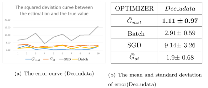
The error in this paper is uniformly expressed by the square of the deviation between the estimator and the true value. Figure Β 2Β  (a) and (b) are the error curve of each estimator and the corresponding error descriptive statistics. As can be seen in Figure 1 (a), the blue curve corresponding to the Β GΒ―m​s​tsubscriptΒ―πΊπ‘šπ‘ π‘‘\bar{G}_{mst}Β  is located at the bottom of all other curves, indicating that the estimated value provided by the Β GΒ―m​s​tsubscriptΒ―πΊπ‘šπ‘ π‘‘\bar{G}_{mst}Β  statistic is the closest to the true value. Figure Β 2Β (b) shows that the error of Β GΒ―m​s​tsubscriptΒ―πΊπ‘šπ‘ π‘‘\bar{G}_{mst}Β  has the smallest mean and standard deviation, indicating that the estimated value provided by Β GΒ―m​s​tsubscriptΒ―πΊπ‘šπ‘ π‘‘\bar{G}_{mst}Β  is more accurate and more stable.

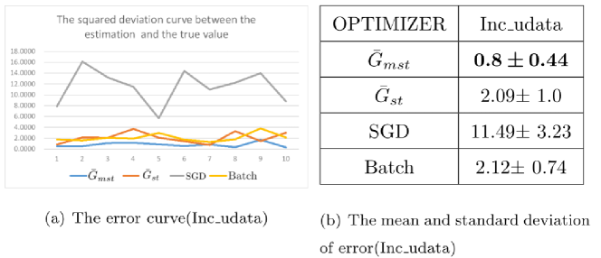
The previous random data set comes from populations with decreasing mean. The second random data is a set of uniformly distributed random numbers from another Β 101010Β  intervalsΒ [0,3],[2,3],[2,4],[3,5],[3,6],[4,7],[5,8],[6,9],[8,10],[8,12]0323243536475869810812[0,3],[2,3],[2,4],[3,5],[3,6],[4,7],[5,8],[6,9],[8,10],[8,12]Β (increasing mean), also be formatted into aΒ 40Γ—10401040\times 10Β matrix as the data population.

It can be seen from FigureΒ 2Β  that on the mean increasing data set, the search direction provided by Β GΒ―m​s​tsubscriptΒ―πΊπ‘šπ‘ π‘‘\bar{G}_{mst}Β  is also satisfactory. For the increasing mean data set, in FigureΒ 2Β  (a), the blue curve corresponding to Β GΒ―m​s​tsubscriptΒ―πΊπ‘šπ‘ π‘‘\bar{G}_{mst}Β  is also located at the bottom of all other curves. In FigureΒ 2Β  (b), the error of Β GΒ―m​s​tsubscriptΒ―πΊπ‘šπ‘ π‘‘\bar{G}_{mst}Β  also has the smallest mean and standard deviation, so the estimated value provided by Β GΒ―m​s​tsubscriptΒ―πΊπ‘šπ‘ π‘‘\bar{G}_{mst}Β is more accurate and more stable.

4.2 Results on normal random data set

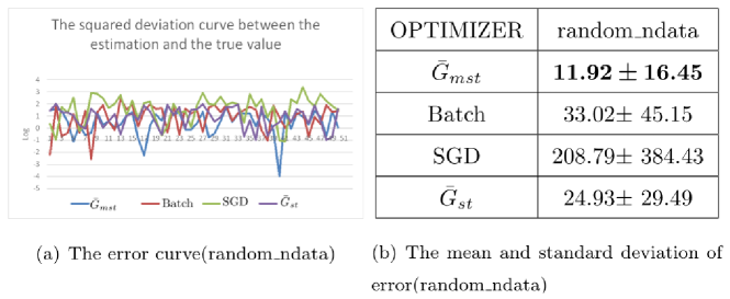
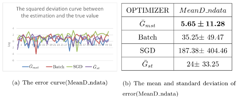
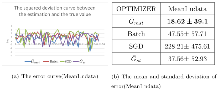
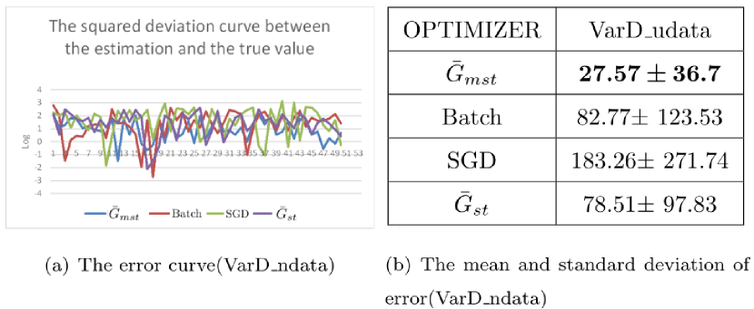
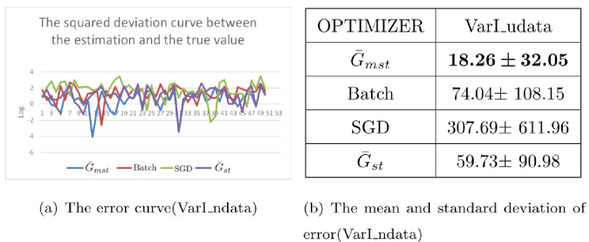
In order to further investigate the performance of the algorithm on other random data sets, this paper generated a set of Β 40Γ—10401040\times 10Β  random numbers from the normal population Β N​(ΞΌ,Οƒ)π‘πœ‡πœŽN(\mu,\sigma)Β  as experimental data. According to the different methods of taking the normal population parameters Β ΞΌ,Οƒπœ‡πœŽ\mu,\sigmaΒ ,five different types of data sets are generated: Β random$\_$ndataΒ (Β ΞΌ,Οƒπœ‡πœŽ\mu,\sigmaΒ are both uniformly distributed random numbers in the interval of [1,20]), Β MeanD$\_$ndataΒ (random data set with decreasing mean), Β MeanI$\_$ndataΒ (random data set with increasing mean), Β VarD$\_$ndataΒ (random data set with decreasing variance), Β VarI$\_$ndataΒ (random data set with increasing variance).

It can be seen from Figure Β 3$\sim$7Β  that whether it is a uniformly distributed random normal data set, or a decreasing mean, increasing mean, decreasing variance, and increasing variance data sets, the gradient estimation value generated by the statistic Β GΒ―m​s​tsubscriptΒ―πΊπ‘šπ‘ π‘‘\bar{G}_{mst}Β  mentioned in this article has the smallest error, and its standard deviation is also the smallest. This shows that the statistic Β GΒ―m​s​tsubscriptΒ―πΊπ‘šπ‘ π‘‘\bar{G}_{mst}Β  can more accurately and stably approximate the gradient mean (true value) of population.

Refer to caption
Figure 3: the error curve and its description statistics(random$\_$ndata)
Refer to caption
Figure 4: the error curve and its description statistics(MeanD$\_$ndata)
Refer to caption
Figure 5: the error curve and its description statistics(MeanI$\_$udata)
Refer to caption
Figure 6: the error curve and its description statistics(VarD$\_$udata)
Refer to caption
Figure 7: the error curve and its description statistics(VarI$\_$udata)

4.3 Results on the MNIST dataset

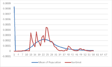
In order to compare the performance differences of different algorithms on the MNIST data set, we use the full gradient method to train a 5-layer forward network with a structure of [784,500, 500,200,10] with a training set of 60,000 scale, with Β Ξ±=0.2𝛼0.2\alpha=0.2Β (step size),$\lambda=0.001$(weight decay coefficient)Β . After 60 iterations, the network achieves 87.73% accuracy on the 10,000-scale test set. We recorded the weight w between the first neuron in the output layer and the first neuron in the penultimate layer, forming the gradient information about 60,000 training samples in 60 iterations, forming a gradient matrix with a scale of Β 60,000Γ—60600006060,000\times 60Β . The average value of each column of the gradient matrix is the true gradient direction of the parameter update.

On the Β 60,000Γ—60600006060,000\times 60Β  gradient matrix, we calculate the expected Β Ejsubscript𝐸𝑗E_{j}Β  and variance Β Vjsubscript𝑉𝑗V_{j}Β  of each category Β j𝑗jΒ  from Β 0∼9similar-to090\sim 9Β , then calculate the Β pj,qjsubscript𝑝𝑗subscriptπ‘žπ‘—p_{j},q_{j}Β of each category according to formulae Β 5Β . Finally, the value of the Β GΒ―m​s​tsubscriptΒ―πΊπ‘šπ‘ π‘‘\bar{G}_{mst}Β  can be calculated using these parameter values.

In order to enhance comparability, except that SGD is a single sample, the sample sizes of Β B​a​t​c​h,GΒ―m​s​t,GΒ―s​tπ΅π‘Žπ‘‘π‘β„ŽsubscriptΒ―πΊπ‘šπ‘ π‘‘subscript¯𝐺𝑠𝑑Batch,\bar{G}_{mst},\bar{G}_{st}Β  are all set to 10. Among them, Β GΒ―m​s​t,GΒ―s​tsubscriptΒ―πΊπ‘šπ‘ π‘‘subscript¯𝐺𝑠𝑑\bar{G}_{mst},\bar{G}_{st}Β  randomly selects a single sample from each of the 10 categories when sampling, and Batch randomly selects 10 samples from 60,000 samples.

The blue curve in Figure Β 8Β  represents the true gradient direction(referred to by Pop in Figure Β 8Β ), which is the average gradient sequence generated by the full gradient method after 60 iterations. The red curve is the curve formed by the gradient sequence generated by 60 iterations of different algorithms. The four sub-graphs show the subtle differences in tracking the direction of the blue curve by the gradient curves generated by different methods.

Refer to caption
(a) GΒ―m​s​tsubscriptΒ―πΊπ‘šπ‘ π‘‘\bar{G}_{mst} VS. Pop.
Refer to caption
(b) $\bar{G}_{st}$ VS. Pop.
Refer to caption
(c) Batch VS. Pop.
Refer to caption
(d) SGD VS. Pop.
Figure 8: Tracing curves of four different estimators to true values

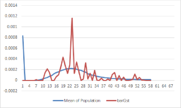
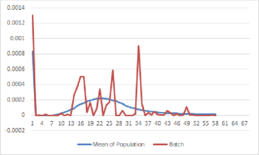
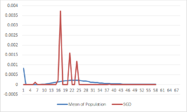
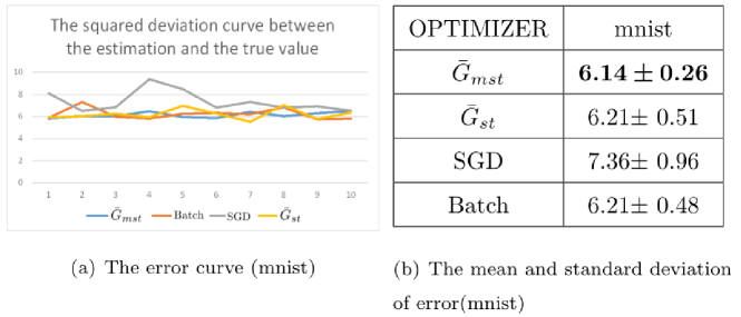
In order to further investigate the accuracy difference of the four methods of Β B​a​t​c​h,S​G​D,GΒ―m​s​t,GΒ―s​tπ΅π‘Žπ‘‘π‘β„Žπ‘†πΊπ·subscriptΒ―πΊπ‘šπ‘ π‘‘subscript¯𝐺𝑠𝑑Batch,SGD,\bar{G}_{mst},\bar{G}_{st}Β , we calculate and record the deviation square of the random gradient direction generated by the four methods and the true gradient direction. Thus, each method obtains 60 such deviation squares, and the average and standard deviation of these 60 deviation squares are used to measure the advantages and disadvantages of the algorithm.

Each algorithm is run repeatedly for 10 times, and the deviation square values generated are recorded. It can be seen from Figure Β 9Β  that even in the case of a small sampling ratio Β f=1060000𝑓1060000f=\frac{10}{60000}Β , the search direction provided by Β GΒ―m​s​tsubscriptΒ―πΊπ‘šπ‘ π‘‘\bar{G}_{mst}Β  is closer to the true value than other methods (the mean and standard deviation of the deviation square are the smallest).

Refer to caption
Figure 9: the error curve and its description statistics(mnist)

we further compare the performance of the four algorithms Β B​a​t​c​h,S​G​D,GΒ―m​s​t,GΒ―s​tπ΅π‘Žπ‘‘π‘β„Žπ‘†πΊπ·subscriptΒ―πΊπ‘šπ‘ π‘‘subscript¯𝐺𝑠𝑑Batch,SGD,\bar{G}_{mst},\bar{G}_{st}Β in optimizing a 5-layer forward network [784,500, 500,200,10]. The data used is still the 60,000-scale MNIST training set and the 10,000-scale MNIST test set. But to be fair, we first implement a grid search procedure for the optimal hyperparameters in the range of alpha=[0.01,1,0.001], lambda=[0.001,0.0001],then examine the training and test accuracy differences of the four algorithms after 1, 2, 3, 4, 5, 6, 7, 8, 9, and 10 thousand iterations under their respective optimal hyperparameters.

TableΒ 1Β  shows the training and testing accuracy achieved by the four algorithms Β B​a​t​c​h,S​G​D,GΒ―m​s​t,GΒ―s​tπ΅π‘Žπ‘‘π‘β„Žπ‘†πΊπ·subscriptΒ―πΊπ‘šπ‘ π‘‘subscript¯𝐺𝑠𝑑Batch,SGD,\bar{G}_{mst},\bar{G}_{st}Β  under their respective optimal hyperparameters. As can be seen from Table Β 1Β , except for 7 and 9 thousand iterations, the training and the test accuracy of Β GΒ―m​s​tsubscriptΒ―πΊπ‘šπ‘ π‘‘\bar{G}_{mst}Β  are the best, outperform than the other four algorithms.

Table 1: Add caption
Iterations SGD(%) GΒ―m​s​tsubscriptΒ―πΊπ‘šπ‘ π‘‘\bar{G}_{mst}(%) Batch(%) $\bar{G}_{st}$(%)
($10^{3}$) test accu train accu test accu train accu test accu train accu test accu train accu
1(SGD:$\times$20) 91.48 91.39 94.46 94.56 93.31 93.38 94.12 94.28
2(SGD:$\times$20) 92.87 92.94 96.05 96.37 95.52 95.88 95.92 96.18
3(SGD:$\times$20) 93.83 94.08 96.53 96.93 96.35 96.86 96.17 96.42
4(SGD:$\times$20) 94.57 94.76 96.74 97.39 96.61 97.25 96.44 96.78
5(SGD:$\times$20) 94.7 94.79 97.17 97.98 97.12 97.81 96.65 97.18
6(SGD:$\times$20) 95.26 95.8 97.3 98.11 97.16 97.91 96.94 97.39
7(SGD:$\times$20) 95.05 95.7 97.13 98.19 97.23 97.89 96.64 97.22
8(SGD:$\times$20) 95.55 95.82 97.65 98.4 97.43 98.33 96.62 97.09
9(SGD:$\times$20) 95.66 96.24 97.41 98.41 97.72 98.49 96.92 97.42
10(SGD:$\times$20) 95.44 95.9 97.63 98.81 97.4 98.45 97.31 97.81

5 Related work

From the update formula Β Ο…t=γ​υtβˆ’1+Ξ·β€‹βˆ‡ΞΈJ​(ΞΈ),ΞΈ=ΞΈβˆ’Ο…tformulae-sequencesubscriptπœπ‘‘π›Ύsubscriptπœπ‘‘1πœ‚subscriptβˆ‡πœƒπ½πœƒπœƒπœƒsubscriptπœπ‘‘\upsilon_{t}=\gamma\upsilon_{t-1}+\eta\nabla_{\theta}J(\theta),\theta=\theta-\upsilon_{t}Β  of the Momentum optimizationΒ [11], the gradient direction required for parameter update in the Momentum optimization is obtained by the weighted summation of the current gradient Β βˆ‡ΞΈJ​(ΞΈ)subscriptβˆ‡πœƒπ½πœƒ\nabla_{\theta}J(\theta) and the historical gradient information stored in Β Ο…tβˆ’1subscriptπœπ‘‘1\upsilon_{t-1}Β  with the weights Β Ξ·,Ξ³πœ‚π›Ύ\eta,\gammaΒ . Here, Β Ξ·,Ξ³πœ‚π›Ύ\eta,\gammaΒ  are similar to that of the parameters q and p, The role of Β Ο…tsubscriptπœπ‘‘\upsilon_{t}Β  is equivalent to the auxiliary variable G in this article. However, the Momentum optimization does not discuss the unbiasedness of Β Ο…tsubscriptπœπ‘‘\upsilon_{t}Β . The results of this paper show that if Β Ξ·,Ξ³πœ‚π›Ύ\eta,\gammaΒ satisfy the Β q,pπ‘žπ‘q,pΒ  conditions in formula Β 5Β , the search direction provided by the Momentum optimization satisfies unbiasedness.

The widely popular Adam algorithmΒ [20]Β  for training deep models,its gradient update formula is Β mt=Ξ²1​mtβˆ’1+(1βˆ’Ξ²1)​gt,m^t=mt1βˆ’Ξ²1formulae-sequencesubscriptπ‘šπ‘‘subscript𝛽1subscriptπ‘šπ‘‘11subscript𝛽1subscript𝑔𝑑subscript^π‘šπ‘‘subscriptπ‘šπ‘‘1subscript𝛽1m_{t}=\beta_{1}m_{t-1}+(1-\beta_{1})g_{t},\hat{m}_{t}=\frac{m_{t}}{1-\beta_{1}}. The parameters Β Ξ²1,(1βˆ’Ξ²1)subscript𝛽11subscript𝛽1\beta_{1},(1-\beta_{1})Β therein are respectively equivalent to the Β p,qπ‘π‘žp,qΒ  parameters in this article. Obviously, according to the results of this article, one of the prerequisites for the effectiveness of Adam’s coefficients Β Ξ²1,(1βˆ’Ξ²1)subscript𝛽11subscript𝛽1\beta_{1},(1-\beta_{1})Β of Β mtβˆ’1,gtsubscriptπ‘šπ‘‘1subscript𝑔𝑑m_{t-1},g_{t}Β  is to ensure that the mean value of the gradients before and after the iterations are equal. Generally, if without additional restrictions, the equal-mean properties of the gradient before and after the iteration are generally not satisfied. Therefore, the author of the Adam algorithm made a so-called unbiased correction Β m^t=mt1βˆ’Ξ²1subscript^π‘šπ‘‘subscriptπ‘šπ‘‘1subscript𝛽1\hat{m}_{t}=\frac{m_{t}}{1-\beta_{1}}Β  on Β mtsubscriptπ‘šπ‘‘m_{t}Β . Obviously, this is an empirical correction formulae, the theoretical basis behind the correction is not fully understood by the authors. In fact, the revised estimator must be a biased estimator, which is contrary to the original intention of the proponent.

The SAG algorithmΒ [13]Β that claims to achieve a linear convergence rate under the condition of strong convexity of the optimization target, the gradient Β fi′​(xk)subscriptsuperscript𝑓′𝑖superscriptπ‘₯π‘˜f^{\prime}_{i}(x^{k})Β  of the current random sample has a proportion of Β 1n1𝑛\frac{1}{n}Β  in the parameter update direction (where n is the total number of training samples), and the remaining ratios are averaged Divided into the gradient of different random samples in different iterations. Here the weight of Β 1n1𝑛\frac{1}{n}Β  is equivalent to the parameter q in this paper. However, SAG roughly assumes that changes in network parameters, such as changes from Β xkβˆ’1superscriptπ‘₯π‘˜1x^{k-1}Β  to Β xksuperscriptπ‘₯π‘˜x^{k}Β , or other forms of change, will not cause fluctuations in the gradient expectations, that is, Β E​(fi′​(xk))=E​(fi′​(xkβˆ’1))𝐸subscriptsuperscript𝑓′𝑖superscriptπ‘₯π‘˜πΈsubscriptsuperscript𝑓′𝑖superscriptπ‘₯π‘˜1E(f^{\prime}_{i}(x^{k}))=E(f^{\prime}_{i}(x^{k-1})). Obviously, the theoretical convergence results obtained on the basis of such assumptions are not firm. Other algorithms such as SAGAΒ [14]Β  and SVRGΒ [15]Β  also explicitly or implicitly acknowledge similar assumptions.

Other variance reduction methods that perform k-step averaging on historical trajectories are equivalent to taking p and q in this article as Β kβˆ’1k,1kπ‘˜1π‘˜1π‘˜\frac{k-1}{k},\frac{1}{k}Β respectively. However, if this approach does not have an additional strategy to limit the gradient to ensure equal gradient mean between different iterations, then the unbiasedness of this approach cannot be satisfied, and the effect of the algorithm will be difficult to guarantee.

References

References

  • [1] Aixiang chen. Deep learning. Tsinghua University press.2020
  • [2] LeCun Y,Bottou L, Bengio Y and Haffner P. Gradient-Based Learning Applied to Document Recognition[J]. Proceedings of IEEE, 1998, 86(11):2278-2324.
  • [3] Ciresan D C,Meier U,Gambardella L M,Schmidhuber J.Deep, big, simple neural nets for handwritten digit recognition[J]. Neural Computation,2010. 22(12): 3207-3220
  • [4] Ciresan D C,Meier U,Masci J,Schmidhuber J.Multi-column deep neural network for traffic sign classification[J]. Neural Networks,2012. 32:333-338.
  • [5] Krizhevsky A,Sutskever I,Hinton G E.ImageNet classification with deep convolutional neural networks[C].Proceedings of International Conference on Neural Information Processing Systems,Lake Tahoe,Nevada,United States,December 3-6,2012:1106–1114.
  • [6] Graves A,FernΓ‘ndez S,Gomez F.Connectionist temporal classification:labelling unsegmented sequence data with recurrent neural networks[C].Proceedings of the 23rd International Conference on Machine Learning,Pittsburgh,PA,USA,2006:369–376.
  • [7] Graves A,Mohamed A,Hinton G E.Speech recognition with deep recurrent neural networks[C].Proceedings of IEEE International Conference on Acoustics, Speech and Signal Processing,Vancouver,BC,Canada,May 26-31,2013:6645-6649.
  • [8] Shillingford B,Assael Y,Hoffman M W,et al.Large-scale visual speech recognition[J].arXiv:1807.05162.
  • [9] Yonghui W,Schuster M, Zhifeng C,et al.Google’s neural machine translation system:bridging the gap between human and machine translation[J].arXiv:1609.08144.
  • [10] Herbert Robbins,Sutton Monro. A Stochastic Approximation Method. Annals of Mathematical Statistics,22(3): 400-407,1951.
  • [11] Ning Qian. On the momentum term in gradient descent learning algorithms.Neural networks.the official journal of the International Neural Network Society, 12(1):145–151, 1999.
  • [12] Yurii Nesterov. A method for unconstrained convex minimization problem with the rate ofconvergence o(1/k2).Doklady ANSSSR (translated as Soviet.Math.Docl.), 269:543–547
  • [13] N. Le Roux, M. Schmidt, and F. Bach. A Stochastic Gradient Method with an Exponential Convergence Rate for Finite Training Sets.Advances in Neural Information Processing System25, pages 2672-2680, 2012.
  • [14] Aaron Defazio, Francis Bach, Simon Lacoste-Julien.SAGA: A Fast Incremental Gradient Method With Support for Non-Strongly Convex Composite Objectives.NIPS, 2014.
  • [15] R. Johnson and T. Zhang. Accelerating stochastic gradient descent using predictive variancereduction.Advances in Neural Information Processing System 26, pages 315-323, 2013
  • [16] Aixiang(Andy) Chen, Xiaolong Chai, Bingchuan Chen, Rui Bian, Qingliang Chen.A novel stochastic stratified average gradient method: Convergence rate and its complexity.in Proceedings of International Joint Conference of Neural Networks(IJCNN),July 2018(arxiv:1710.07783V3).
  • [17] John Duchi, Elad Hazan, and Yoram Singer. Adaptive Subgradient Methods for Online Learning and Stochastic Optimization.Journal of Machine Learning Research, 12:2121–2159, 2011
  • [18] Matthew D. Zeiler.ADADELTA: An Adaptive Learning Rate Method.arXiv preprint arXiv:1212.5701,2012
  • [19] Tijmen Tieleman and Geoffrey Hinton. 2012. Lecture 6.5-rmsprop: Divide the gradient by a running average of its recent magnitude. COURSERA: Neural networks for machine learning, 4(2):26–31.
  • [20] Diederik P. Kingma and Jimmy Lei Ba. Adam: a Method for Stochastic Optimization.International Conference on Learning Representations, pages 1–13, 2015.
  • [21] Timothy Dozat. Incorporating Nesterov Momentum into Adam.ICLR Workshop, (1):2013–2016,2016.
  • [22] Sashank J. Reddi, Satyen Kale, and Sanjiv Kumar. On the convergence of adam and beyond. In Proceedings of International Conference on Learning Representations.2018
  • [23] B. T. Polyak and A. Juditsky. Acceleration of stochastic approximation by averaging.SIAM Journalon Control and Optimization, 30:838–855, 1992.
  • [24] Yu. Nesterov. Primal-dual subgradient methods for convex problems.Mathematical Programming,120(1):221–259, 2009. Appeared early as CORE discussion paper 2005/67, Catholic Universityof Louvain, Center for Operations Research and Econometrics.