Universal Approximation Under Constraints is Possible with Transformers

Abstract

Many practical problems need the output of a machine learning model to satisfy a set of constraints, $K$. There are, however, no known guarantees that classical neural networks can exactly encode constraints while simultaneously achieving universality. We provide a quantitative constrained universal approximation theorem which guarantees that for any convex or non-convex compact set $K$ and any continuous function $f:\mathbb{R}^{n}\rightarrow K$, there is a probabilistic transformer $\hat{F}$ whose randomized outputs all lie in $K$ and whose expected output uniformly approximates $f$. Our second main result is a “deep neural version” of Berge (1963)’s Maximum Theorem. The result guarantees that given an objective function $L$, a constraint set $K$, and a family of soft constraint sets, there is a probabilistic transformer $\hat{F}$ that approximately minimizes $L$ and whose outputs belong to $K$; moreover, $\hat{F}$ approximately satisfies the soft constraints. Our results imply the first universal approximation theorem for classical transformers with exact convex constraint satisfaction, and a chart-free universal approximation theorem for Riemannian manifold-valued functions subject to geodesically-convex constraints.

Keywords: Constrained Universal Approximation, Probabilistic Attention, Transformer Networks, Geometric Deep Learning, Measurable Maximum Theorem, Non-Affine Random Projections.

1 Introduction

In supervised learning, we select a parameterized model $\hat{f}:{\mathbb{R}}^{n}\rightarrow{\mathbb{R}}^{m}$ by optimizing a real-valued loss function$L$ over training data from an input-output domain $\mathcal{X}\times\mathcal{Y}\subseteq{\mathbb{R}}^{n}\times{\mathbb{R}}^{m}$. A necessary property for a model class to produce asymptotically optimal results, for any continuous loss $L$, is the universal approximation property. However, often more structure (beyond vectorial ${\mathbb{R}}^{m}$) is present in a learning problem and this structure must be encoded into the trained model $\hat{f}$ to obtain meaningful or feasible predictions. This additional structure is typically described by a constraint set $K\subseteq{\mathbb{R}}^{m}$ and the condition $\hat{f}(\mathcal{X})\subseteq K$. For example, in classification $K=\{y\in[0,1]^{m}:\,\sum_{i=1}^{m}y_{i}=1\}$ (Shalev-Shwartz & Ben-David, 2014), in Stackelberg games (Holters et al., 2018; Jin et al., 2020; Li et al., 2021) $K$ is the set of utility-maximizing actions of an opponent, in integer programming $K$ is the integer lattice ${\mathbb{Z}}^{m}$ (Conforti et al., 2014), in financial risk-management $K$ is a set of positions meeting the minimum solvency requirements imposed by international regularity bodies (Basel Committee on Banking Supervision, 2015; 2019; McNeil et al., 2015), in covariance matrix prediction $K\subseteq{\mathbb{R}}^{m\times m}$ is the set of $m\times m$ matrices which are symmetric and positive semi-definite (Bonnabel et al., 2013; Bonnabel & Sepulchre, 2009; Baes et al., 2021), in geometric deep learning $K$ is typically a manifold (e.g. a pose manifold in computer vision and robotics (Ding & Fan, 2014) or a manifold of distance matrices (Dokmanic et al., 2015)), a graph, or an orbit of a group action (Bronstein et al., 2017; 2021; Kratsios & Bilokopytov, 2020). Therefore, we ask:

Is exact constraint satisfaction possible with universal deep learning models?

The answer to this question begins by examining the classical universal approximation theorems for deep feedforward networks. If $L$ and $K$ are mildly regular, the universal approximation theorems of Hornik et al. (1989); Cybenko (1989); Pinkus (1999); Gühring et al. (2020); Kidger & Lyons (2020); Park et al. (2021) guarantee that for any “good activation function $\sigma$” and for every tolerance level $\epsilon>0$, there is a deep feedforward network with activation function $\sigma$, such that $\inf_{y\in K}\,L(x,y)$ and $L(x,\hat{f}(x))$ are uniformly at most $\epsilon$ apart. Written in terms of the optimality set,

$$\sup_{x\in\mathcal{X}}\|\hat{f}(x)-\underset{{\color[rgb]{0.0,0.2,0.13}{y\in K}}}{\operatorname{argmin}}\,L(x,y)\|{\color[rgb]{0.03,0.27,0.49}{\leq\epsilon}},$$ (1)

where the distance of a point $y\in{\mathbb{R}}^{m}$ to a set $A\subseteq{\mathbb{R}}^{m}$ is defined by $\|y-A\|\triangleq\inf_{a\in A}\|y-a\|$. Since $\operatorname{argmin}_{y\in K}L(x,y)\subseteq K$, then (1) only implies that $\|\hat{f}(x)-K\|\leq\epsilon$ and there is no reason to believe that the constraint $\hat{f}(x)\in K$ is exactly satisfied, for every $x\in\mathcal{X}$.

This kind of approximate constraint satisfaction is not always appropriate. In the following examples constraint violation causes either practical or theoretical concerns:

1. In post-financial crisis risk management, international regulatory bodies mandate that any financial actor should maintain solubility proportional to the risk of their investments (Basel Committee on Banking Supervision, 2015; 2019). To prevent future financial crises, any violation of these risk constraints, no matter the size, incurs large and immediate fines.

2. In geometric deep learning, we often need to encode complicated non-vectorial structure present in a dataset, by viewing it as a $K$ valued function (Fletcher, 2013; Bonnabel & Sepulchre, 2009; Baes et al., 2021). However, if $K$ is non-convex then Motzkin (1935) confirms that there is no unique way to map predictions $\hat{f}(x)\not\in K$ to a closest point in $K$. Thus, we are faced with the dilemma: either make an ad-hoc choice of a $k$ in $K$ with $k\approx\hat{f}(x)$ (ex.: an arbitrary choice scheme when $K={\mathbb{Z}}^{m}$) or have meaningless predictions (ex: non-integer values to integer programs, or symmetry breaking (Weinberg, 1976)).

Constrained learning was recognized as an effective framework for fairness and robustness by Chamon & Ribeiro (2020) who study empirical risk minimization under constraints. Many emerging topics in machine learning lead to constrained learning formulations. A case in point is model-based domain generalization (Robey et al., 2021). Despite the importance of (deep) learning with constraints, there are no related approximation-theoretic results to the best of our knowledge.

In this paper, we bridge this theoretical gap by showing that universal approximation with exact constraint satisfaction is always possible for deep (probabilistic) transformer networks with a single attention mechanism as output layer. Our contribution is three-fold:

1. We derive the first universal approximation theorem with exact constraint satisfaction;

2. Our transformer network’s encoder and decoder adapt to the dimension of the constraint set and thus beat the curse of dimensionality for low-dimensional constraints;

3. Our models leverage a probabilistic attention mechanism that can encode non-convex constraints. This probabilistic approach is key to bypass the topological obstructions to non-Euclidean universal approximation (Kratsios & Papon, 2021).

Our analysis provides perspective on the empirical success of attention and adds to the recent line of work on approximation theory for transformer networks, (Yun et al., 2020a; b), which roughly considers the unconstrained case (with $K$ in (1) replaced by ${\mathbb{R}}^{m}$) in the special case of $L(x,y)=\|f(x)-y\|$ for a suitable target function $f:{\mathbb{R}}^{n}\rightarrow{\mathbb{R}}^{m}$. Our probabilistic perspective on transformer networks fits with the representations of Vuckovic et al. (2021) and of Kratsios (2021).

Our results can be regarded as an approximation-theoretic counterpart to the constrained statistical learning theory of Chamon & Ribeiro (2020). Further, they put forward a perspective on randomness in neural networks that is complementary to the work of Louart et al. (2018); Gonon et al. (2020a; b). We look at the same problem focusing on constraint satisfaction instead of training efficiency. Finally, our proof methods are novel, and build on contemporary tools from metric geometry (Ambrosio & Puglisi, 2020; Bruè et al., 2021).

1.1 The Probabilistic Attention Mechanism

We now give a high-level explanation of our results; the detailed formulations are in Section 2.

Introduced in (Bahdanau et al., 2015) and later used to define the transformer architecture (Vaswani et al., 2017), in the NLP context, attention maps a matrix of queries $Q$, a matrix of keys $K$, and a matrix of values $V$ to the quantity $\operatorname{Softmax}(QK^{\top})V$, where the softmax function (defined below) is applied row-wise to $QK^{\top}$. Just as the authors of (Petersen & Voigtlaender, 2020; Zhou, 2020) focus on the simplified versions of practically implementable ConvNets in the study of approximation theory of deep ConvNets (e.g. omitting pooling layers), we find it sufficient to study the following simplified attention mechanism to obtain universal approximation results:

$$\operatorname{Attention}\left(w,Y\right)\triangleq\operatorname{Softmax}_{N}\left(w\right)^{\top}Y=\sum_{n=1}^{N}[\operatorname{Softmax}_{N}(w)_{n}]Y_{n},$$ (2)

where $w\in{\mathbb{R}}^{N}$, $\operatorname{Softmax}_{N}:{\mathbb{R}}^{N}\ni w\mapsto(\frac{e^{w_{k}}}{\sum_{j=1}^{N}e^{w_{j}}})_{k=1}^{N}$, and $Y$ is an $N\times m$ matrix. The attention mechanism (2) can be interpreted as “paying attention” to a set of particles $Y_{1},\dots,Y_{N}\in{\mathbb{R}}^{m}$ defined by $Y$’s rows. This simplified form of attention is sufficient to demonstrate that transformer networks can approximate a function while respecting a constraint set, $K$, whether convex or non-convex.

Informal Theorem 1.1 (Deep Maximum Theorem for Transformers).

If $K$ is convex and the quantities defining (1) are regular then, for any $\epsilon\in(0,1]$, there is a feedforward network $\hat{f}$, an ${\mathcal{X}_{\epsilon}}\subset{\mathbb{R}}^{n}$ of probability $1\mbox{-}\epsilon$, and a matrix $Y$ such that the transformer $\operatorname{Attention}(\hat{f}(x),Y)$ satisfies:

1. Exact Constraint Satisfaction: For each $x\in{\mathbb{R}}^{n}$, $\operatorname{Attention}(\hat{f}(x),Y){\color[rgb]{0.0,0.2,0.13}{\in K}}$,

2. Universal Approximation: $\sup_{x\in\mathcal{X}_{\epsilon}}\,\|\operatorname{Attention}(\hat{f}(x),Y)-\underset{{\color[rgb]{0.0,0.2,0.13}{y^{\star}\in K}}}{\operatorname{argmin}}\,L(x,y^{\star})\|{\color[rgb]{0.03,0.27,0.49}{\leq\epsilon}}$

Informal Theorem 1.1 guarantees that simple transformer networks can minimize any loss function while exactly satisfying the set of convex constraints. As illustrated by Figure 1 and Figure 2, $K$’s convexity is critical here, since without it the transformer’s prediction may fail to lie in $K$. This is because any transformer network’s output is a convex combinations of the particles $Y_{1},Y_{2},Y_{3}$; thus, any transformer network’s predictions must belong to these particles’ convex hull.

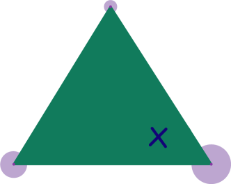
Figure 1: Convex Constraints

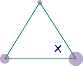
Figure 2: Non-Convex Constraints

In Figures 1 and 2, $Y$’s columns, i.e. the particles $Y_{1},Y_{2}$, and $Y_{3}$, are each illustrated by a $\bullet$ at the constraint set ($K$) vertices. The bubble around each each $Y_{i}$ illustrates the predicted probability, for a given input, that $f(x)$ is nearest to that $Y_{i}$. The $\bm{\times}$ is the transformer’s prediction which is, by construction, a convex combination of the $Y_{i}$ weighted by the aforementioned probabilities and therefore they lie in the $K$ if it is convex (Figure 1) but not if $K$ is non-convex (Figure 2).

Naturally, we arrive at the question: How can (i) and (ii) simultaneously hold when $K$ is non-convex?

Returning to Vaswani et al. (2017) and using the introduced terminology, we note that the role of the $\operatorname{Softmax}_{N}$ layer is to rank the importance of the particles $\{Y_{n}\}_{n=1}^{N}$ when optimizing $L$, at any given input: the weights $[\operatorname{Softmax}_{N}(w)]_{n}$ in (2) can be interpreted as charging their respective point masses $\{\delta_{Y_{n}}\}_{n=1}^{N}$ with probabilities of being optimal for $L$ (relative to the other particles). This suggests the following probabilistic reinterpretation of attention (which we denote by p-attention):

$$\operatorname{P-attention}(w,Y)\triangleq\sum_{n=1}^{N}[\operatorname{Softmax}_{N}(w)]_{n}\delta_{Y_{n}}.$$ (3)

Crudely put, $\operatorname{P-attention}(\cdot,Y)$ “pays relative attention to the particles” $Y_{1},\dots,Y_{n}\in{\mathbb{R}}^{m}$.

A simple computation shows that the mean prediction of our probabilistic attention mechanism, exactly implements “classical” $\operatorname{Attention}$ of Vaswani et al. (2017), as defined in (2),

$$\operatorname{Attention}(w,Y)=\mathbb{E}_{X\sim\operatorname{P-attention}(w,Y)}[X],$$ (4)

where $\mathbb{E}_{X\sim\operatorname{P-attention}(w,Y)}[X]$ denotes the (vector-valued) expectation of a random-vector $X$ distributed according to $\operatorname{P-attention}(w,Y)$. Hence, (3) is no less general than (2). The advantage of (3) is that, if each particle $Y_{n}$ belongs to $K$ (even if $K$ is non-convex) then, any sample drawn from the probability measure $\operatorname{P-attention}(w,Y)$ necessarily belongs to $K$.

1.2 Qualitative Results: Deep Maximum Theorem

Probabilistic attention (3) yields the following non-convex generalization of Informal Theorem 1.1. The result is a qualitative universal approximation theorem as well as a deep neural version of the Maximum Theorem (Berge, 1963), which states that under mild regularity conditions, given any well-behaved family of input dependent “soft constraint sets” $\{C_{x}\}_{x\in{\mathbb{R}}^{n}}$ compatible with $K$, there is a measurable function mapping each $x\in{\mathbb{R}}^{n}$ to a minimizer of $L(x,y)$ on $K\cap C_{x}$.

We use ${\mathscr{W}}_{1}$ to denote the Wasserstein-1 distance between probability measures on $K$. The results also give the flexibility to the user to enforce an input-dependent family of “soft constraints” $\{C_{x}\}_{x\in{\mathbb{R}}^{n}}$ which only need to hold approximately; definitions are provided in Section 1.4.

Informal Theorem 1.2 (Deep Maximum Theorem: Non-Convex Case).

If the quantities defining 1 are regular, $K$ is a compact set of “exact constraints”, and $\{C_{x}\}_{x\in{\mathbb{R}}^{n}}$ a set of “soft constraints”, then, for any approximation quality $0<\epsilon\leq 1$, there is a deep feedforward network $\hat{f}$ and a matrix $Y$ satisfying:

1. Exact Constraint Satisfaction: For each $x\in{\mathbb{R}}^{n}$, $\operatorname{P-attention}(\hat{f}(x),Y)$ is supported in $K$,

2. Universal Approximation: ${\mathbb{P}}({\mathscr{W}}_{1}(\operatorname{P-attention}(\hat{f}(x),Y),\underset{{y^{\star}\in C_{x}\cap K}}{\operatorname{argmin}}\,L(x,y^{\star}))\leq\epsilon)\geq 1-\epsilon;$

where for a probability measure ${\mathbb{P}}$ on ${\mathbb{R}}^{m}$ and a $B\subseteq{\mathbb{R}}^{m}$ we define ${\mathscr{W}}_{1}({\mathbb{P}},B)\triangleq\inf_{b\in B}\,{\mathscr{W}}_{1}({\mathbb{P}},\delta_{b})$.

Example 1.3 (Reduction to Classical Point-to-Set Distance).

In particular, when ${\mathbb{P}}$ is a point-mass ${\mathbb{P}}=\delta_{y}$ for some $y\in{\mathbb{R}}^{m}$, then one recovers the familiar Euclidean distance to the set $B$ via:

$${\mathscr{W}}_{1}(\delta_{y},B)\overset{\operatorname{(def)}}{=}\inf_{b\in B}\,{\mathscr{W}}_{1}(\delta_{y},\delta_{b})=\inf_{b\in B}\,\|y-b\|\overset{\operatorname{(def)}}{=}\|y-B\|;$$

where the first and second equality follows from (Villani, 2009, (5) - page 99), and the last equality is the definition of $\|y-B\|$ (as in (Aubin & Frankowska, 2009, Definition 1.1.1)).

Another important class of non-convex constraints arising from geometric deep learning where $K$ is a non-Euclidean ball in a Riemannian submanifold of ${\mathbb{R}}^{m}$. In this broad case, we may extract mean predictions from $\operatorname{P-attention}(\hat{f},Y)$, by applying the Fréchet mean introduced in Fréchet (1948). Such “geometric means” are well-understood theoretically (Bhattacharya & Patrangenaru, 2003) and easily handled numerically Miolane et al. (2020); Lou et al. (2020).

1.3 Quantitative Results: Constrained Universal Approximation Theorem

In its current form, the objective function $L$ is too general to derive quantitative approximation rates. Nevertheless, as with most universal approximation theorems (Hornik et al., 1989; Pinkus, 1999; Kidger & Lyons, 2020), if each soft constraint $C_{x}$ is set to ${\mathbb{R}}^{m}$ and $L$ quantifies the uniform distance to an unknown continuous function $f:{\mathbb{R}}^{n}\rightarrow K$ in the Euclidean sense,

$$L(x,y)\triangleq\|f(x)-y\|,$$

then, Informal Theorem 1.2 reduces to a (qualitative) universal approximation for transformer networks with exact constraint satisfaction. In fact, this additional structure is enough for us to derive quantitative versions of the aforementioned results. We permit ourselves the general situation, where $K$ is contained in an unknown $d$-dimensional submanifold (where $d\in\Theta(m^{\frac{1}{s}})$ for some $s>0$). Our approximation rates scale favourably in the ratio $s\approx\frac{\log(m)}{\log(d)}$; i.e., we avoid the curse of dimensionality for low-dimensional constraint sets. This additional structure translates into the familiar encoder-decoder structure deployed in most transformer network implementations.

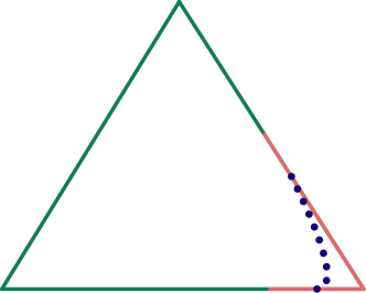
Figure 3: Encoder : $\approx$ $f$

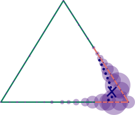
Figure 4: Decoder : $\approx$ Random Projection to $K$

Figure 3 illustrates the encoder network $\hat{\mathcal{E}}:{\mathbb{R}}^{n}\rightarrow{\mathbb{R}}^{m}$, whose role is to perform a (classical) unconstrained approximation of the target function, $f$. Since $\hat{\mathcal{E}}$ is a classical feedforward network then its approximation of the target function can be arbitrarily close to the constraint set $K$ but it need not lie in it. The next step is to “map the encoder network’s output onto $K$ with low distortion.”

The role of the decoder network $\hat{\mathcal{D}}$ is to correct any constraint violation made by encoder network by “projecting them back on to $K$”. However, such a projection does not exist if $K$ is not convex since there must be more than one closest point in $K$ to some $y\in{\mathbb{R}}^{m}$ (Motzkin, 1935). Nevertheless, if the “projection” were capable of mapping any $y\in{\mathbb{R}}^{m}$ to multiple points on $K$, ranked by their proximity to $y$, then there would be no trouble. The decoder network accomplishes precisely this, as illustrated in Figure 4, where the bubbles illustrate the probability of any particle in $K$ being closest to ${\color[rgb]{0,0,1}{y}}$, illustrated by the size of the bubbles in Figure 4. Mathematically, $\hat{\mathcal{D}}:{\mathbb{R}}^{m}\rightarrow\mathcal{P}_{1}(K)$ approximates a (non-affine) random projection, in the sense of Ohta (2009); Ambrosio & Puglisi (2020); Bruè et al. (2021); i.e.: a $1$-Lipschitz map $\Pi:{\mathbb{R}}^{m}\rightarrow\mathcal{P}_{1}(K)$ satisfying the random projection property: for all $y\in K$

$$\Pi_{y}=\delta_{y}.$$

Thus, $\Pi$’s random projection property means that it fixes any output already satisfying the constraint $K$, and its Lipschitz regularity implies that it is stable. Thus, sampling from $\Pi(y_{1})$ is similar to sampling from $\Pi(y_{2})$ whenever the points $y_{1},y_{2}\in{\mathbb{R}}^{m}$ are near to one another.

Remark 1.4.

Random projections are closely tied to the (random) partitions of unity of Lee & Naor (2005) (see (Ambrosio & Puglisi, 2020, Theorem 2.8)). These random projections generalize the random projections of Johnson & Lindenstrauss (1984), beyond the case where $K$ is affine.

Remark 1.5.

The special case of random projections onto affine spaces has recently been used when constructing universal neural models (Cuchiero et al., 2021; Puthawala et al., 2020).

We record the complexity of both the decoder and encoder networks constructed in our quantitative results in Table 1. Here $A,B,C,D\geq 0$ are constants independent of $\epsilon$ and $k$, where $k\in{\mathbb{N}}_{+}$ is the number of continuous derivatives which $f$ admits (when viewed as a function into ${\mathbb{R}}^{m}$).

Network	$\hat{\mathcal{E}}$	$\hat{\mathcal{D}}$
Depth	$\mathscr{O}(m^{\frac{1}{s}}(1+\epsilon^{\frac{2n}{3(kn+1)}-\frac{2n}{kn+1}}))$	$\mathscr{O}\left((N^{\frac{3}{2}}(A+2\epsilon)(4-\epsilon^{-1})^{2})^{\frac{2m}{s}}\right)$
Width	$m^{\frac{1}{s}}(4n+10)$	$m^{\frac{1}{s}}+N+2$
$N$	-	$\mathscr{O}\left((\epsilon^{-1}A+B)^{\frac{m}{2}}\right)$
$Q$	-	$\mathscr{O}\left(\epsilon^{\frac{-m}{s}}\right)$

Table 1: Complexity of simple transformer network $\hat{f}=\hat{\mathcal{D}}\circ\hat{\mathcal{E}}$ approximating $f$.

From Table 1, we see that if $m^{\frac{1}{s}}\ll m$ then, $s>0$ is large; hence, $\epsilon^{\frac{m}{s}}$, $(1-4\epsilon^{-1})^{\frac{2m}{s}}$, and $N^{\frac{m}{s}}$ are small.

1.4 Notation and Background

Optimal Transportd

Given any non-empty subset $K\subseteq{\mathbb{R}}^{m}$, the set of all Borel probability measures ${\mathbb{P}}$ on $K$ with a finite mean; i.e.: $\mathbb{E}_{X\sim{\mathbb{P}}}[\|X\|]<\infty$, is denoted by $\mathcal{P}_{1}(K)$. Wasserstein distance ${\mathscr{W}}_{1}$ is defined for any ${\mathbb{P}},{\mathbb{Q}}\in\mathcal{P}_{1}(K)$ by the minimal energy needed to transport all mass from ${\mathbb{P}}$ to ${\mathbb{Q}}$. Following Villani (2009), ${\mathscr{W}}_{1}({\mathbb{P}},{\mathbb{Q}})$ is defined by:

$${\mathscr{W}}_{1}({\mathbb{P}},{\mathbb{Q}})\triangleq\inf_{\pi}\mathbb{E}_{(X_{1},X_{2})\sim\pi}[\|X_{1}-X_{2}\|],$$

where the infimum is taken over all Borel probability measures $\pi$ on $K^{2}$ with marginals ${\mathbb{P}}$ and ${\mathbb{Q}}$. The metric space $(\mathcal{P}_{1}\left({K}\right),{\mathscr{W}}_{1})$ is named the Wasserstein space over $K$; we abbreviate it by $\mathcal{P}_{1}\left({K}\right)$.

Smooth Function Spaces

The set of real-valued continuous functions on ${\mathbb{R}}^{n}$ is denoted by $C({\mathbb{R}}^{n})$. Let $k\in{\mathbb{N}}_{+}$ and $\mathcal{X}\subseteq[0,1]^{n}$ be non-empty. The set of functions $f:\mathcal{X}\rightarrow K$ for which there is a $k$-times continuously differentiable $\bm{f}:{\mathbb{R}}^{n}\rightarrow{\mathbb{R}}^{m}$ extending $f$; i.e.: $\bm{f}|_{\mathcal{X}}=f$, is denoted by $C_{tr}^{k}(\mathcal{X},K)$. Our interest in $C_{tr}^{k}(\mathcal{X},K)$ does not stem from the fact that it contains all smooth functions mapping $[0,1]^{n}$ to $K$, but rather that it allows us to speak about the uniform approximation of discontinuous $K$-valued functions on regions in $[0,1]^{n}$ where they are “regular”. This is noteworthy for pathological constraint sets, such as integer constraints. For details on $C_{tr}^{k}(\mathcal{X},K)$, see (Brudnyi & Brudnyi, 2012a; b) and the extension theorems of Whitney (1934); Fefferman (2005).

Neural Networks

It has recently been observed that deep feedforward networks with multiple activation functions, or more generally parametric families of activation functions, achieved significantly more efficient approximation rates than classical feedforward networks with a single activation function (Yarotsky & Zhevnerchuk, 2020; Yarotsky, 2021; Shen et al., 2021a; b). Practically deployed examples of parametric activation functions are the PReLU activation function of He et al. (2015), the Sigmoid-weighted Linear Unit (SiLU) of Elfwing et al. (2018), and the Swish activation function of Ramachandran et al. (2018). We also observe a similar phenomenon, and therefore our quantitative results consider deep feedforward networks whose activation functions belongs to a $1$-parameter family $\sigma_{\star}\triangleq\{\sigma_{t}\}_{t\in[0,1]}\subseteq C({\mathbb{R}})$. The set of all such networks is denoted by $\mathcal{NN}_{n,N}^{\sigma_{\star}}$ and it includes all $\hat{f}:{\mathbb{R}}^{n}\rightarrow{\mathbb{R}}^{N}$ with iterative representation:

$$\hat{f}(x)\triangleq A^{(J)}x^{(J)},\qquad x^{(j+1)}_{i_{j}}\triangleq\sigma_{t_{i_{j}}}((A^{(j)}x)_{i_{j}}+b^{(j)}_{i_{j}}),\qquad x^{(0)}\triangleq x,$$ (5)

where $x\in{\mathbb{R}}^{n}$, $j=1,\dots,J-1$, each $A^{(j)}$ is a $d_{j}\times d_{j+1}$-matrix, each $b^{(j)}\in{\mathbb{R}}^{d_{j+1}}$, $d_{J+1}=N$, $d_{1}=0$, $t_{1,1},\dots,t_{J,N_{J}}\in[0,1]$, for each $j$. The integer $J$ is $\hat{f}$’s depth and $\underset{j=1,\dots,{J+1}}{\max}d_{j}$ is $\hat{f}$’s width.

Example 1.6 (Networks with Untrainable Nonlinearity).

Denote $\sigma\triangleq\sigma_{0}$. The subset of classical feedforward networks consisting of all $\hat{f}\in\mathcal{NN}_{n,N}^{\sigma_{\star}}$ with each $\sigma_{t_{i_{j}}}=\sigma$ in (5) is denoted $\mathcal{NN}_{n,N}^{\sigma}$.

It is approximation theoretically advantageous to generalize the proposed definition of probabilistic attention in the introduction (3) by replacing $Y$ with a $3$-dimensional array (elementary $3$-tensor).

Definition 1.7 (Probabilistic Attention).

Let $N,Q,m\in{\mathbb{N}}_{+}$, and $Y$ be an $N\times Q\times m$-array with $Y_{n,q}\in K$ for $n=1,\dots,N$, $q=1,\dots,Q$. Probabilistic attention is the function:

$${\mathbb{R}}^{n}\ni w\mapsto\operatorname{P-attention}(w,Y)\triangleq\frac{1}{Q}\sum_{n=1}^{N}\sum_{q=1}^{Q}\operatorname{Softmax}_{N}(w)_{n}\delta_{Y_{n,q}}\in\mathcal{P}_{1}\left({K}\right).$$

If $Y$ is an $N\times m$-matrix, as in (3), then we identify $Y$ as the $N\times m\times 1$-array in the obvious manner.

Set-Valued Analysis:

A family of non-empty subsets $\{C_{x}\}_{x\in{\mathbb{R}}^{n}}$ of $K$ is said to be a weakly measurable correspondence, denoted $C:{\mathbb{R}}^{n}\rightrightarrows{\mathbb{R}}^{m}$, if for every open subset$U\subseteq K$, $\{x\in{\mathbb{R}}^{n}:\,C_{x}\cap U\neq\emptyset\}$ is a non-empty Borel subset of ${\mathbb{R}}^{n}$ (Aliprantis & Border, 2006, pages 557, 592).

2 Main Results

We now present our main results in detail. All proofs are relegated to the paper’s appendix.

2.1 Qualitative Approximation: Deep Maximum Theorem

Our main qualitative result is the following deep neural version of Berge (1963)’s Maximum Theorem where, the measurable selector is approximately implemented by a probabilistic transformer network. We first present the general qualitative result which gives a concrete description of a measurable selector of (1), with high-probability, which has the key property that all its predictions satisfy the required constraints defined by $K$.

Assumption 2.1 (Kidger & Lyons (2020)).

$\sigma:{\mathbb{R}}\rightarrow{\mathbb{R}}$ is continuous, $\sigma$ is differentiable at some $x_{0}\in{\mathbb{R}}$, and its derivative satisfies $\sigma^{\prime}(x_{0})\neq 0$.

Theorem 2.2 (Deep Maximum Theorem).

Let $\sigma$ satisfy Assumption 2.1. Let $K\subseteq{\mathbb{R}}^{n}$ be a non-empty compact set, $C:{\mathbb{R}}^{n}\rightrightarrows{\mathbb{R}}^{m}$ be a weakly-measurable correspondence with closed values such that $C_{x}\cap K\neq\emptyset$ for each $x\in{\mathbb{R}}^{n}$, $L\in C({\mathbb{R}}^{m})$, and $\mathbb{P}$ be a Borel probability measure on ${\mathbb{R}}^{n}$. For each $0<\epsilon\leq 1$, there is an $N\in{\mathbb{N}}_{+}$, an $\hat{f}\in\mathcal{NN}_{n,N}^{\sigma}$ of width at most $2+n+N$, and an $N\times m$-matrix $Y$ such that:

$$\smash{\hat{F}:\mathbb{R}^{n}\ni x\mapsto\operatorname{P-attention}\left(\hat{f}(x),Y\right)\in\mathcal{P}_{1}({\mathbb{R}}^{m}),}$$ (6)

satisfies the following:

1. Exact Constrain Satisfaction: $\cup_{x\in{\mathbb{R}}^{n}}\,\operatorname{supp}(\hat{F}(x))\subseteq K$,

2. Probably Approximately Optimality: There is a compact ${\mathcal{X}_{\epsilon}}\subseteq{\mathbb{R}}^{n}$ satisfying:

   1. $\underset{x\in{\mathcal{X}_{\epsilon}}}{\max}\,{\mathscr{W}}_{1}(\hat{F}(x),\underset{{y\in C_{x}\cap K}}{\operatorname{argmin}}\,L(x,y))\leq\epsilon,$

   2. $1-{\mathbb{P}}({\mathcal{X}_{\epsilon}})\leq\epsilon.$

Theorem 2.2 implies that for any random field $(Y^{x})_{x\in{{{\mathbb{R}}^{n}}}}$ on ${{{\mathbb{R}}^{m}}}$ (i.e. a family of ${{{\mathbb{R}}^{m}}}$-valued random vectors indexed by ${\mathbb{R}}^{n}$) with $Y^{x}\sim\hat{F}(x)$: 1. samples drawn from $Y^{x}$ are in $K$ (by (i)) and 2. samples drawn from each $Y^{x}$ are near to the optimality set $\operatorname{argmin}_{y\in C_{x}\cap K}L(x,y)$ (by (ii)).

Corollary 2.3 ($\hat{F}$’s Mean Prediction).

Assume the setting of Theorem 2.2. Let $\{Y^{x}\}_{x\in{\mathbb{R}}^{n}}$ be a $K$-valued random field with $Y^{x}\sim\hat{F}(x)$ for each $x\in{\mathbb{R}}^{n}$ then, $1-{\mathbb{P}}({\mathcal{X}_{\epsilon}})\leq\epsilon$ and

$$\underset{x\in{\mathcal{X}_{\epsilon}}}{\max}\,\mathbb{E}[\|Y^{x}-\underset{{y^{\star}\in C_{x}\cap K}}{\operatorname{argmin}}\,L(x,y^{\star})\|]\leq\epsilon.$$

Appendix 8 contains additional consequences of the Deep Maximum Theorem, such as the special case of classical transformers when $K$ is convex. Next, we complement our qualitative results by their quantitative analogues, within the context of universal approximation under constraints.

2.2 Quantitative Approximation: Constrained Universal Approximation

In order to derive a quantitative constrained universal approximation theorem, we require the loss function to be tied to the Euclidean norm in the following manner.

Assumption 2.4 (Norm-Controllable Loss).

There is a continuous $f:{\mathbb{R}}^{n}\rightarrow{\mathbb{R}}^{m}$ with $f({\mathbb{R}}^{n})\subseteq K$ and a continuous $l:[0,\infty)\rightarrow[0,\infty)$ with $l(0)=0$, satisfying: $L(x,y)\leq l(\|f(x)-y\|).$

Just as with transformer networks, our “constrained universal approximation theorem” approximates a suitably regular function $f:{\mathbb{R}}^{n}\rightarrow K\subseteq{\mathbb{R}}^{m}$ while exactly respecting the constraints $K$ by implementing an encoder-decoder network architecture. Thus, our model is a composition of an encoder network $\hat{\mathcal{E}}:{\mathbb{R}}^{n}\rightarrow{\mathbb{R}}^{d}$ whose role is to approximate $f$ in a classical “unconstrained fashion” and a decoder network (with probabilistic attention layers at its output) $\hat{\mathcal{D}}:{\mathbb{R}}^{d}\rightarrow\mathcal{P}_{1}(K)$ whose role is to enforce the constraints $K$ while preserving the approximation performed by $\hat{\mathcal{E}}$, where $d\lll m$.

To take advantage of the encoder-decoder framework present in most transformer networks, we formalize what is often called a “latent low-dimensional manifold” hypothesis. Briefly, this means that, the hard constraints in set $K$ are contained in a “low dimensional” subspace.

Assumption 2.5 (Low-Dimensional Manifold).

There is an $0<s$ and a smooth bijection $\Phi$ from ${\mathbb{R}}^{n}$ to itself with smooth inverse, such that $\Phi(K)\subseteq{\mathbb{R}}^{d}$; where $2\leq d$ and $d\in\Theta(m^{\frac{1}{s}})$.

Assumption 2.5 does not postulate that $K$ is itself a single-chart low-dimensional manifold, or even a manifold. Rather, $K$ need only be contained in a low-dimensional manifold. For the fast rates we use activation functions generalizing the swish function (Ramachandran et al., 2018) as follows.

Assumption 2.6 (Swish-Like Activation Function).

The map $\sigma:[0,1]\times{\mathbb{R}}\ni(\alpha,t)\mapsto\sigma_{\alpha}(t)\in{\mathbb{R}}$ is continuous; $\sigma_{0}$ is non-affine and piecewise-linear, and $\sigma_{1}$ is smooth and non-polynomial.

Theorem 2.7 (Constrained Universal Approximation).

Let $k\in{\mathbb{N}}_{+}$ and $\mathcal{X}\subseteq[0,1]^{n}$ be non-empty. Suppose that $\sigma$ satisfies 2.6, $L$ satisfies Assumption 2.4, $K\subseteq{\mathbb{R}}^{n}$ is non-empty, compact and satisfies Assumption 2.5. For any $f\in C_{tr}^{k}(\mathcal{X},K)$, every constraining quality $\epsilon_{K}>0$, and every approximation error $\epsilon_{f}>0$, there exist $N,Q\in{\mathbb{N}}_{+}$, an encoder $\hat{\mathcal{E}}\in\mathcal{NN}_{n,d}^{\sigma}$, and a decoder:

$$\hat{\mathcal{D}}:{\mathbb{R}}^{d}\ni x\mapsto\sum_{k=1}^{N}\operatorname{P-attention}\left(\hat{D}(x),Y\right)\in\mathcal{P}_{1}(K)$$ (7)

where $\hat{D}\in\mathcal{NN}_{d,N}^{\sigma}$ and $Y$ is an $N\times Q\times m$-array with $Y_{1,1},\dots,Y_{N,Q}\in K$ such that:

1. Exact Constrain Satisfaction: For each $x\in{\mathbb{R}}^{n}$: $\operatorname{supp}(\hat{\mathcal{D}}\circ\hat{\mathcal{E}}(x))\subseteq K,$

2. Universal Approximation: The estimate holds :

   $$\sup_{x\in[0,1]^{n}}\,{\mathscr{W}}_{1}(\hat{\mathcal{D}}\circ\hat{\mathcal{E}}(x),\underset{y\in K}{\operatorname{argmin}}\,L(x,y))\leq\epsilon_{K}+k\operatorname{Lip}(\Phi^{-1})d\epsilon_{f};$$

   where, $0<k$ is an absolute constant independent of $n$, $m$, $d$, $f$, and of $\epsilon$ and $\operatorname{Lip}(\Phi^{-1})$ denotes the Lipschitz constant of $\Phi^{-1}$ on the compact set $\{z\in{\mathbb{R}}^{d}:\,\|z-\Phi(K)\|\leq\epsilon_{f}\}$.

Furthermore, the “complexities” of $\hat{\mathcal{D}}$ and $\hat{\mathcal{E}}$ are recorded in Table  1 for $\frac{\epsilon}{2}=\epsilon_{k}=\epsilon_{f}$.

In practice, we can only sample from each measure $\hat{\mathcal{D}}\circ\hat{\mathcal{E}}(x)$. In this case, we may ask how the typical sample drawn from a random-vector $Y^{x}$ distributed according to our learned measure $\hat{\mathcal{D}}\circ\hat{\mathcal{E}}(x)$ performs when minimizing $L(x,y)$. The next result relates the estimates in Theorem 2.7 (ii) to the typical (in $Y^{x}$) worst-case (in $x$) gap between a sample from $Y^{x}$ and $f(x)$, as quantified by $L(x,\cdot)$.

Corollary 2.8 (Average Worst-Case Loss).

Assume the setting of Theorem 2.7 and suppose that the “modulus” $l$ in Assumption 2.4 is strictly increasing and concave. Let $\hat{\mathcal{D}}$ and $\hat{\mathcal{E}}$ be as in Theorem 2.7 and let $\{Y^{x}\}_{x\in\mathcal{X}}$ be an ${\mathbb{R}}^{m}$-valued random field with $Y^{x}\sim\hat{\mathcal{D}}\circ\hat{\mathcal{E}}(x)$, for each $x\in{\mathbb{R}}^{n}$. Then:

$$\underset{x\in\mathcal{X}}{\max}\,\mathbb{E}_{Y^{x}\sim\hat{\mathcal{D}}\circ\hat{\mathcal{E}}(x)}\left[L(x,Y^{x})\right]\leq l\left(\epsilon_{K}+k\operatorname{Lip}(\Phi^{-1})d\epsilon_{f}\right).$$

Corollary 2.8 quantifies the expected performance of a sample from our probabilistic transformer model, as expressed by $L$, whereas Theorem 2.7 (ii) quantifies the difference from the transformer’s prediction to the optimal prediction value. Next, we consider implications of our main results.

2.3 Applications

We apply our theory to obtain a universal approximation theorem for classical transformer networks with exact convex constraint satisfaction and to derive a version of the non-Euclidean universal approximation theorems of Kratsios & Bilokopytov (2020); Kratsios & Papon (2021) for Riemannian-manifold valued functions which does not need explicit charts. As with most quantitative (uniform) universal approximation theorems (Gühring et al., 2020; Kidger & Lyons, 2020; Shen et al., 2021a), we henceforth consider $L(x,y)=\|f(x)-y\|$. We also fix $f\in C_{tr}^{k}([0,1]^{n},K)$.

2.3.1 Transformers are Convex-Constrained Universal Approximators

We return to the familiar transformer networks of Vaswani et al. (2017). The next result shows that transformer networks can balance universal approximation and exact convex constraint satisfaction. This is because when $K$ is convex, then the mean of the random field $\{Y^{x}\}_{x\in{\mathbb{R}}^{n}}$ of Corollary 2.3 must belong to $K$. Consequently, the identity (4) implies that $\operatorname{Attention}(\hat{\mathcal{D}}\circ\hat{\mathcal{E}}(\cdot),Y)\approx f$.

Corollary 2.9 (Constrained Universal Approximation: Convex Constraints).

Consider the setting and notation of Corollary 2.8. Suppose that $K$ is convex and let $L(x,y)=\|f(x)-y\|$. Then:

$$\smash{{\mathbb{R}}^{n}\ni x\mapsto\mathbb{E}[Y^{x}]=\operatorname{Attention}(\hat{\mathcal{D}}\circ\hat{\mathcal{E}}(x),Y)\in K;}$$ (8)

1. Exact Constraint Satisfaction: $\mathbb{E}_{Y^{x}\sim\hat{\mathcal{D}}\circ\hat{\mathcal{E}}(x)}[Y^{x}]\in K$, for each $x\in{\mathbb{R}}^{n}$,

2. Universal Approximation: $\sup_{[0,1]^{n}}\,\|f(x)-\mathbb{E}_{Y^{x}\sim\hat{\mathcal{D}}\circ\hat{\mathcal{E}}(x)}[Y^{x}]\|<\epsilon_{K}+kd\epsilon_{f}.$

The “complexities” of the networks $\hat{\mathcal{D}}$ and $\hat{\mathcal{E}}$ are recorded in Table  1 for $\frac{\epsilon}{2}=\epsilon_{k}=\epsilon_{f}$.

2.3.2 Chart-Free Riemannian Manifold-Valued Universal Approximation

We explore how additional non-convex structure of the constraint set $K$ can be encoded by the probabilistic transformer networks of Theorems 2.2 and 2.7 and be used to build new types of (deterministic) transformer networks. These results highlight that the standard transformer networks of (8) are specialized for convex constraints and that by instead using an intrinsic variant of expectation, we build can new types of “geometric transformer networks” customized to $K$’s geometry. This section makes use of Riemannian geometry; for an overview see Jost (2017).

Let $(M,g)$ be a connected $d$-dimensional Riemannian submanifold of ${\mathbb{R}}^{m}$ with distance function by $d_{g}$. We only require the following mild assumption introduced in Afsari (2011). We recall that the injectivity radius at $y_{0}$, denoted by $\operatorname{inf}_{g}(y_{0})$, (see (Jost, 2017, Definition 1.4.6)) is the minimum length of a geodesic (or minimal length curve) in $M$ with starting point $y_{0}$. We also recall that the sectional curvature (see (Jost, 2017, Definition 4.3.2) for a formal statement) quantifies the curvature of $(M,g)$ as compared the geometry of its flat counterpart ${\mathbb{R}}^{d}$. We focus on a broad class of non-convex constrains, namely geodesically convex constraints, which generalize convex constraint and have received recent attention in the optimization literature (Zhang & Sra, 2016; Liu et al., 2017).

Assumption 2.10 (Geodesically Convex Constraints).

The Riemannian manifold $(M,g)$ is connected, it is complete as a metric space, and all its sectional curvatures of $(M,g)$ are all bounded above by a constant $C\geq 0$. The non-empty constrain set $K$ satisfies:

1. $K$ is contained in the geodesic ball $B(y_{0},\rho)\triangleq\{y\in M:\,d_{g}(y_{0},y)<\rho\}$ for some point $y_{0}\in M$ and some radius $\rho$ satisfying: $0<\rho<2^{-1}\min\{\operatorname{inj}_{g}(y_{0}),\frac{\pi}{\sqrt{C}}\},$

2. For each $y_{0},y_{1}\in K$ there exists a unique geodesic $\gamma:[0,1]\rightarrow K$ joining $y_{0}$ to $y_{1}$.

Our latent probabilistic representation grants us the flexibility of replacing the usual “extrinsic mean” used in (8) to extract deterministic predictions from our probabilistic transformer networks via an additional Fréchet mean layer at their readout. This intrinsic notion of a mean, was introduced independently in Fréchet (1948) and in Karcher (1977), and is defined on any $\mathbb{P}\in\mathcal{P}_{1}(K)$ by:

$$\bar{\mathbb{P}}\triangleq\underset{k\in K}{\operatorname{argmin}}\,\int\,d_{g}^{2}(k,u)\,\mathbb{P}(du).$$ (9)

With this “geometric readout layer” added to our model, we obtain the following variants of our main results in this non-convex, but geometrically regular, setting.

Corollary 2.11 (Constrained Universal Approximation: Riemannian Case).

Consider the setting and notation of Corollary 2.8. Let $L(x,y)=\|f(x)-y\|$. If Assumption 2.10 holds then:

$${\mathbb{R}}^{n}\ni x\mapsto\overline{\hat{\mathcal{D}}\circ\hat{\mathcal{E}}(x)}\in K,$$ (10)

is a well-defined Lipschitz-continuous function, and the following hold:

1. Exact Constraint Satisfaction: $\overline{\hat{\mathcal{D}}\circ\hat{\mathcal{E}}(x)}\in K$, for each $x\in\mathcal{X}$,

2. Universal Approximation: $\sup_{\mathcal{X}}\,d_{g}(f(x),\overline{\hat{\mathcal{D}}\circ\hat{\mathcal{E}}(x)})<\epsilon_{K}+kd\epsilon_{f}.$

The “complexities” of $\hat{\mathcal{D}}$ and $\hat{\mathcal{E}}$ are recorded in Table 1 for $\frac{\epsilon}{2}=\epsilon_{k}=\epsilon_{f}$.

3 Discussion

In this paper, we derived the first constrained universal approximation theorems using probabilistic reformation of Vaswani et al. (2017)’s transformer networks. The results assumed both a quantitative form (Theorem 2.7) and a qualitative form in the more general case of an arbitrary loss functions $L$ and additional compatible soft constraints in (Theorem 2.2). Our results provide (generic) direction to end-users designing deep learning models processing non-vectorial structures and constraints.

As this is the first approximation theoretic result in this direction, there are naturally as many questions raised as have been answered. In particular, it is natural to ask: “Are the probabilistic transformer networks trainable in practice; especially when $K$ is non-convex?”. In Appendix 5, we show that the answer is indeed: “Yes!”, by proposing a training algorithm in that direction and showing that we outperform an MLP model and a classical transformer network in terms of a joint MSE and distance to the constraint set. The evaluation is performed on a large number of randomly generated experiments, whose objective is to reduce the MSE to a randomly generated function mapping a high-dimensional Euclidean space to there sphere ${\mathbb{R}}^{3}$ with outputs constrained to the sphere.

4 Precise Transformer Complexities and Approximation Rates

This section records the exact approximation rates, or equivalently the precise model complexities, of the transformer networks implemented in our quantitative constrained universal approximation results. The rates are simply those recorded in Table 1 but with explicit constants.

Table 2 makes use of the following notation. We denote the diameter of the compact set $K$ by $\operatorname{diam}(K)\triangleq\max_{y_{1},y_{2}\in K}\,\|y_{1}-y_{2}\|$. Furthermore, $k>0$ in Table 2 is a universal constant independent of $\epsilon_{K}$, $\epsilon_{f}$, $f$, $K$, $n$, $m$, and of $d$. The big $\mathscr{O}$ notation used in Table 2 masks any constants not depending on these quantities.

Network $\hat{\mathcal{E}}$ $\hat{\mathcal{D}}$ Depth $\mathscr{O}(m^{\frac{1}{s}}(1+\epsilon_{f}^{\frac{2n}{3(kn+1)}-\frac{2n}{kn+1}}))$ $\mathscr{O}\left((m^{\frac{1}{s}}N^{\frac{3}{2}}(\operatorname{Lip}(\Phi)\operatorname{diam}(K)+2\epsilon_{f})(1-\frac{\epsilon_{K}^{-1}}{4})^{2}(1+\frac{m^{\frac{1}{s}}}{4}))^{\frac{2m}{s}}\right)$ Width $\mathscr{O}(m^{\frac{1}{s}}(4n+10))$ $\mathscr{O}(m^{\frac{1}{s}}+N+2)$ $N$ - $\mathscr{O}\left(\left(\frac{km^{\frac{2}{s}}2^{\frac{9}{2}}\operatorname{Lip}(\Phi)(\operatorname{diam}(K)+\epsilon_{f})}{\sqrt{m^{\frac{1}{s}}+1}\epsilon_{K}}\right)^{\frac{m}{s}}\right)$ $Q$ - $\mathscr{O}\left((\epsilon_{K}^{-1}\operatorname{Lip}(\Phi)\operatorname{diam}(K)m^{\frac{5}{2s}})^{\frac{m}{s}}\right)$

Table 2: Complexities of encoder-decoder Network with P-attention for $0<\epsilon_{K}\leq 1$.

Remark 4.1.

If $\epsilon_{K}>1$ then the above rates hold but the term $(1-\frac{\epsilon_{K}^{-1}}{4})^{2}$ in $\hat{\mathscr{D}}$’s depth estimate must be replaced by $(1-\frac{\epsilon_{K}^{-1}}{4})(1-\epsilon_{K}^{-1})$ in order for the rates to remain valid.

5 Can the Probabilistic Transformer Network be Trained?

The purpose of this appendix is to answer the following questions:

1. Are our probabilistic transformer networks trainable and, if so, how?

2. How do probabilistic transformer networks perform on a toy non-convex problem?

We first affirm (i) by describing a potential training algorithm for our model. Then, we address (ii) on a toy non-convex problem whose objective is to learn (randomly generated) functions taking values on the standard $2$-sphere in ${\mathbb{R}}^{3}$. Our code is available at code is available at Anonymized (2021).

5.1 A Training Algorithm

Our analysis only has practical implications as we can affirmatively answer the following question:

“Is the probabilistic transformer network $$\hat{F}$$ of Theorem 2.7 trainable?”

Our theoretical analysis motivates the following training procedure, whose steps we briefly explain.

Step 1 - Get Particles:

We assume that the user is has access to a subroutine $\operatorname{Generate}$ which generates particles on $K$. This is always possible, for example, by randomly by sampling the available training outputs $\{y_{t}\}_{t=1}^{T}$; for example, this is what is done in our toy implementations. However, if one has access to additional structure, such as a $K$-supported probability measure (Miolane et al., 2020) then, samples can be drawn therefrom, or if $K$ is equipped with a meaningful metric, then the randomized partition procedure such as (Bartal, 1999; Pulat, 1989) can be deployed.

Step 2 - Train Model:

When $m>1$, the Wasserstein distance is costly to evaluate numerically (Pele & Werman, 2009; Cuturi, 2013; Kolouri et al., 2019; Sommerfeld et al., 2019). A variety of approximate or regularized transport distances have been introduced to manage this problem but only approximately. However, in the context of Theorem 2.7 and Algorithm 1 we are always interested in distances to the pointmass and therefore, ${\mathscr{W}}_{1}$ has the following exceptional closed-form expression which bypasses these computational issues:

$$\sum_{t=1}^{T}\mathcal{W}_{1}(\delta_{f(x_{t})},\operatorname{P-attention}(\hat{f}(x_{t}),Y))=\sum_{t=1}^{T}\sum_{n=1}^{N}\left\|y_{t}-Y_{n}\right\|[\operatorname{Softmax}_{N}\circ\hat{f}(x_{t})]_{n}.$$ (11)

Remark 5.1 (Exceptional Closed-Form for $\mathcal{W}_{1}(\delta_{f(x_{t})},\operatorname{P-attention}(\hat{f}(x_{t}),Y))$ in (11)).

A derivation of the closed-form identity 11 is in Lemma 6.4.

Step 2 - Prediction:

In the case where $K$ is a Riemannian manifold, Since Fréchet means are readily implemented in a variety of packages (Miolane et al., 2020), we assume that the user has access to a subroutine $\operatorname{Fr\mbox{\'{e}}chet\,Mean}$ which takes an $N\times Q$-matrix of weights $(w_{n,q})_{n,q=1}^{N,Q}$ and an $N\times Q\times 1$-array and computes the Fréchet mean (9). By Corollary 2.11, once the network $\hat{F}$ is trained, its outputs generate points on $K$ via the Fréchet mean (9); i.e.: $\overline{\hat{F}(x)}=\operatorname{argmin}_{y\in K}\sum_{n,q=1}^{N,Q}w_{n,q}d_{g}^{2}(y,y_{n,q}).$

Input: Training Data $\{(x_{t},y_{t})\}_{t=1}^{T}\subseteq{\mathbb{R}}^{n}\times K$

Output: Probabilistic Transformer Network: $\hat{F}\triangleq\sum_{n=1}^{N}\sum_{q=1}^{Q}[\operatorname{Softmax}_{N}\circ f(\cdot)]_{n}w_{n,q}\delta_{y_{n,q}}$

1 Get Particles: Use $\operatorname{Generate}$ $K$ to generate $y_{1},\dots,y_{S}\in K$

for $n=1,\dots,N$ do

      $\{s_{q}\}_{q=1}^{Q}\leftarrow\operatorname{argsort}_{Q}\,\{\|y_{s}-Y_{n}\|\}_{s=1}^{S}$

      $\{y_{n,q}\}_{q=1}^{Q}\leftarrow\{y_{s_{q}}\}_{q=1}^{Q}$

      endfor for

     2Train Model:

     Get Labels: for $t\leq T$ do

           for $n\leq N$ do

                $(L_{t})_{n}\leftarrow I(\|y_{t}-Y_{n}\|\leq\min_{m=1,\dots,N}\|y_{t}-Y_{m}\|$)

                endfor for

               

                endfor for

               3$\hat{f}\leftarrow\operatorname{argmin}_{\hat{f}}\sum_{t=1}^{T}\sum_{n=1}^{N}\|(L_{t})_{n}-[\operatorname{Softmax}_{N}\circ\hat{f}(x_{t})]_{n}\|^{2}$

return $\hat{F}(\cdot)\triangleq\sum_{n=1}^{N}\operatorname{Softmax}_{N}\circ\hat{f}(\cdot)_{n}\delta_{Y_{n}}$

Algorithm 1 Training Probabilistic Transformers for Exact Constraint Satisfaction

Remark 5.2 (Prediction).

Predictions can be made using $\hat{F}$ by either applying an expectation, in which case classical tranformer networks of Vaswani et al. (2017) are recovered, using the Fréchet mean as a final layer if $K$ is a geodesically convex subset of a Riemannian submanifold of $\mathbb{R}^{m}$, or taking the most-likely particle if noting more is known of $K$ other than its point-set.

We now address question (ii).

5.2 Performance on a Toy Non-Convex Problem

Let $K\subseteq{\mathbb{R}}^{2}$ be a $2$-dimensional sphere in ${\mathbb{R}}^{3}$. Let $a,b,c$ be independently drawn from a uniform distribution on $[0,1]$ and let $A$ be a $2\times{10^{3}}$ random matrix with i.i.d. standard Gaussian entries. Let $f=\tilde{f}(Ax)$ be the random $K$-valued function where $u_{i}=ax^{2}_{i}+bx_{i}+c$, for $i=1,2$, and $\tilde{f}(u)\triangleq(\cos(\tilde{f}(u)_{1})\sin(\tilde{f}(u)_{2})),\sin(\tilde{f}(u)_{1})\sin(\tilde{f}(u)_{2})),\cos(\tilde{f}(u)_{1})\cos(\tilde{f}(u)_{2})))$. Therefore, $A$ projects ${\mathbb{R}}^{{10^{3}}}$ onto the latent low-dimensional space ${\mathbb{R}}^{2}$ and $\tilde{f}$ sends data in ${\mathbb{R}}^{2}$ to a point on the sphere obtain by a random polynomial transformation of its spherical coordinates (which is a non-convex constraint set).

We independently repeat this experiment $500$-times, generating a random $f$ each time and generating $1k$ training inputs $\{x_{t}\}_{t=1}^{{10^{3}}}\subseteq[0,1]^{{10^{3}}}$ (resp. $100$ testing inputs) by independently and uniformly sampling from $[0,1]^{{10^{3}}}$ and producing $1k$ corresponding training (resp. $100$ testing) outputs $\{f(x_{t})\}_{t=1}^{{10^{3}}}\subset K$. For each independent experiment, a probabilistic transformer network ${\mathbb{P}}\mbox{-Trans.}$) is trained using Algorithm 1, and benchmarked against a deep feedforward network (MLP) and a classical transformer network (Trans.). Table 3 reports the average and standard deviation, across all experiments, of the test-set MSE and the distance to the constraint set ($d_{K}$) of the test-set predictions for each learning model.

Figure 5 shows that, high emphasis is placed on constraint satisfaction ($\lambda\in[0,0.75]$) then the ${\mathbb{P}}$-Trans.+Fréchet model outperforms the benchmark models. As the emphasis parameter $\lambda$ approaches the critical value of $\approx.75$ then, the MSE dominates the constraint satisfaction metric $d_{K}$ and the ${\mathbb{P}}$-Trans.+Fréchet’s larger average test MSE is larger than that of the MLP and Trans. models. This validates the error terms $\epsilon_{K}$ and the factor $k\operatorname{Lip}(\Phi^{-1})d$ in Theorem 2.7 (ii), reflected in Table 3, which is due to the decoder network $\hat{\mathcal{D}}$ in $f$ approximating a random projection of ${\mathbb{R}}^{3}$ onto $K$.

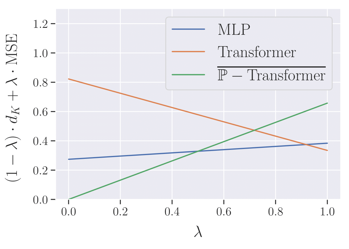
Figure 5: Performance for varying importance on constraint satisfaction vs. MSE.

Therefore, we find that our probabilistic transformer network is both implementable, and that, as expected, it offers good predictive performance even while enforcing non-convex constrained. In other words, we have obtained positive answers to the natural questions (i) and (ii) posed at the start of Appendix 5.

	$d_{K}$		MSE
	Mean	Std	Mean	Std
MLP	0.274	0.106	0.384	0.034
Transformer	0.822	0.100	0.334	0.009
$\overline{{\mathbb{P}}\mbox{-Transformer}}$	0.000	0.000	0.657	0.059

Table 3: Performance metrics across all $500$ experiments.

Table 3 emphasizes that classical transformer networks are not built to handle non-convex constraints. Indeed, the poor performance of the transformer network, with respect to the $d_{K}$, is due to most its predictions lying inside the sphere (which is hollow).

Further study into training algorithms for our model, and detailed ablation of the model parameters are topics of focus in forthcoming research. Nevertheless, we have obtained an affirmative answer to both our questions (i) and (ii). Namely, we have shown that our probabilistic transformer morel is trainable via a simple procedure such as Algorithm 1.

5.3 Examining the impact of $K$’s Geometry on Transformer Networks

To gain further insight into how probabilistic transformers encode geometric priors, we will examine the impact of perturbations to $K$ on the probabilistic transformer’s approximation capabilities. We consider toy illustrations beginning with the convex setting before moving on to the fully non-convex setting where no projections, charts, or even a Riemannian structure is available.

We further underline that step $3$ in Algorithm 1 may be performed in a variety of ways and, unlike the previous experiments, all networks in this section are obtained by randomizing their hidden weights and only training their final layer. Theoretical guarantees for this approach has become relatively well understood (Louart et al., 2018; Gonon et al., 2020a; b). Implicitly, our examples also show that probabilistic transformers can equally be integrated into domains where randomized models such as extreme learning machines (ELMs) are typical; e.g. in the reservoir computing Lukoševičius & Jaeger (2009); Grigoryeva & Ortega (2018; 2019).

This section’s primary goal is to experimentally validate the main quantitative claim made implicitly in our main result; i.e. Theorem 2.7. Namely, we verify that:

“The model complexities in Table 1 are independent of $$K$$’s geometry.”

That is, the approximation quality of any optimized probabilistic transformer network only depends on the involved dimensions. Expressed another way, we empirically validate our result that the probabilistic transformer networks can encode any geometric prior with the model complexity agnostic of $K$’s geometry.

Accordingly, all model architectures’ hyperparameters are kept fixed across all experiments. Each experiment reports the probabilistic transformer’s MSE relative to the benchmark MLP model $\left(\frac{\mbox{MSE}}{\mbox{MSE-MLP}}\right)$.

Our result is validated upon observing that the probabilistic transformer model’s $\frac{\mbox{MSE}}{\mbox{MSE-MLP}}$ is of the same order across all experiments. In other words: probabilistic transformers can approximate a $K$-valued function while simultaneously encoding $K$’s geometry with the same efficiency as an MLP trained only to approximate $f$ that ignores $K$’s geometry.

Each toy experiment is trained on a dataset of $900$ instances and tested on a dataset of $100$ instances. We maintain the coloring scheme of Figure 5 in all our subsequent plots, namely the MLP is colored in blue, the Transformer is colored in orange, and the ${\mathbb{P}}\mbox{-Transformer}$ is colored in green.

5.3.1 Convex Constraints

Our first set of examples concern the case where $K$ is a convex constraint set, as studied in Corollaries 2.9. In each instance, we generate a random target function $f$, mapping ${\mathbb{R}}^{2}$ to $K$. The function $f$ is defined via the following two-step procedure:

$$f:\mathbb{R}\overset{\tilde{f}}{\rightarrow}\mathbb{R}^{2}\overset{P_{K}}{\rightarrow}{\color[rgb]{0.0,0.2,0.13}{K}};$$

where $\tilde{f}:{\mathbb{R}}^{2}\ni x\mapsto Ax$ is a random rotation matrix re-scaled by a factor of $1.5$ with the angle sampled uniformly from $[0,2\pi]$ and where $P_{K}:{\mathbb{R}}^{2}\ni x\mapsto\operatorname{argmin}_{y\in K}\,\|y-x\|$ is the metric projection onto the $K$, which exist in this context by (Motzkin, 1935). Figures 6 and  9 illustrate this two step transformation by first representing the uniformly generated input data in violet then, illustrating their images under $\tilde{f}$ in light green, and finally plotting their value under $f$ in dark green.

We perform our illustrations in the visualizable two dimensional case where $K$ is either the square $[-1,1]^{2}$ or the disk $\{y\in{\mathbb{R}}^{2}:\,\|y\|\leq 1\|$. This is because the projection operators ($P_{K}$) are readily interpretable from their closed-form formulations (Bauschke & Combettes, 2011). Respectively, these are given by $P_{K}(x)=(\min\{\max\{x_{i},-1\},1\})_{i=1}^{2}$ and $P_{K}(x):=\frac{x}{\max\{1,\|x\|\}}$.

Figures 7 and 10 demonstrate the constraint set ($K$) in green and the particles, which populate $Y$’s rows, in violet. These are generated randomly by first sampling uniformly from $[-2,2]^{2}$ and then projecting each sample onto $K$ via $P_{K}$. Figures 7 and 10 illustrate the role of the particles defining the probabilistic attention mechanism, defined in (3); namely, they identify the points in $K$ on which any output may approximately lie. Thus, the role of the encoder and decoder networks can be summarized as learning to classify which input is closest to which particle.

Figure 6: $x\mapsto f(x)$.

Figure 7: Particles $(Y)$ on Constraint Set $(K)$.

Therefore, at high-level, the probabilistic attention mechanism 3 quantizes the constraint set $K$. The (simplified) classical Attention mechanism of (4) implements a (convex) interpolation between the particles quantizing $K$ and an analogous statement is true of Riemannian analogue (Section 2.3.2). For general $K$, however, such interpolations within $K$ can be impossible or unclear how to implement them. Nevertheless, the probabilistic attention mechanism never faces such a difficulty since it explicitly “interpolates” in $\mathcal{P}_{1}(K)$ and not on $K$ directly.

Figure 8: Performance: MSE vs. $d_{K}$.

$\frac{\mbox{MSE}}{\mbox{MSE MLP}}$ MSE $d_{K}$ MLP 1 4.35e-04 7.39e-03 Transformer 4.81 1.20e-02 0.00e+00 $\overline{{\mathbb{P}}\mbox{-Transformer}}$ 4.01 5.86e-03 0.00e+00

Table 4: Performance Metrics

We obtain analogous results to the $500$ experiments performed in the case where $K$ is geodesically-convex in Section 5.2. Just as in Figure 5, Figures 8 and 11 show that the transformer can simultaneously encode $K$ and approximate $f$, wheras the MLP cannot. More precisely, in each case, if at-least roughly equal importance is placed on predictive accuracy (MSE) and constraint satisfaction ($d_{K}$) then, the transformer models offer the best performance. This is equally reflected in the test set performance metrics of Tables 5.3.1 and 5.3.1 which are consistent with the findings of Table 3.

Figure 9: $x\mapsto f(x)$.

Figure 10: Particles $(Y)$ on the constraint set $(K)$.

At times, when $K$’s geometric is sufficiently simple we the transformer can outperform the probabilistic transformer. This is not surprising, since Corollary 2.9 guaranteed that the transformer universal in this setting an exactly implements the $K$’s geometry. Nevertheless, in both instances, the MLP cannot compete when encoding the geometric prior defined by the constraint set $K$.

Figure 11: Performance: MSE vs. $d_{K}$.

$\frac{\mbox{MSE}}{\mbox{MSE MLP}}$ MSE $d_{K}$ MLP 1 4.09e-04 4.75e-03 Transformer 2.98 3.87e-03 0.00e+00 $\overline{{\mathbb{P}}\mbox{-Transformer}}$ 3.41 4.50e-03 6.11e-19

Table 5: Performance Metrics

5.3.2 Fully Non-Convex Constraints

Let us study the milieu in which probabilistic transformer is the only universal approximator capable of constraint satisfaction (unlike the case where $K$ is convex and we showed that the transformer filled this role). Specifically, we consider the case where $K$ does not admit a single chart (since it has non-trivial homotopy), nor is there a well-defined projection operator of some ${\mathbb{R}}^{m}$ onto $K$.

Analogously to the convex situation investigated in Section 5.3.1, we define

$$f:\mathbb{R}\overset{\tilde{f}}{\rightarrow}\mathbb{R}\overset{\rho}{\rightarrow}{\color[rgb]{0.0,0.2,0.13}{K}};$$

where $\tilde{f}(x)\triangleq\sum_{i=0}^{5}\beta_{i}x^{i}$ is a (random) quintic polynomial function with $\beta_{i}\sim N(0,1)$, and the constraint set’s geometry is defined by $K$; where $\rho:{\mathbb{R}}\rightarrow{\mathbb{R}}^{2}$. In this experiment, we also allow the training data to be perturbed by multivariate Gaussian noise with variance $10^{-1}$.

Similarly to Figures 6 and 9, in Figures 12 and 15, we use a color coded visualization method to understand $f$. Sample points from $[-10,10]$ and label them with a color gradient ranging from pink to blue such that pinkish points are close to $-10$ and blueish points are a nearer to $10$. The image ($f(x)$ of each input ($x$) on $K$ is illustrated using the same colour as $x$ did. This coloring helps us visualize the winding of $f$ around $K$.

Nevertheless, as in the convex case, we can generate particles on $K$ by first sampling from $[-10,10]$ and then mapping them onto $K$ using $\rho$. Thus, even if no chart or projection operator is available, we can easily build probabilistic attention mechanisms.

Figure 12: $x\mapsto f(x)$.

Figure 13: Particles $(Y)$ on Constraint Set $(K)$.

In Figures 12 and 13, the map defining $K$’s geometry is $\rho(y)\triangleq(2\cos(y)^{2}+1)\cdot(\cos(y/3),\sin(y/3))$. Figure 14 and Table 5.3.2 show that our probabilistic transformer network’s performance is “robust to changes of geometric priors”, in the sense that the relative performance of our models is entirely analogous to the above experiments where $K$ was convex or it was a geodesically convex patch on a Riemannian manifold.

Figure 14: Performance: MSE vs. $d_{K}$.

$\frac{\mbox{MSE}}{\mbox{MSE MLP}}$ MSE $d_{K}$ MLP 1 2.40e+00 6.56e-01 Trans. 1.01 2.51e+00 3.98e-01 ${\mathbb{P}}\mbox{-Trans.}$ 1.05 2.76e+00 0.00e+00

Table 6: Performance Metrics

We complete our discussion by considering an instance where $K$’s geometry is both non-convex and it is not a differentiable manifold (due to the self-intersecting point). This last toy example is illustrated in Figures 15 and 16 in which case $K$’s geometry is the image of the map $\rho(y)\triangleq\Phi(\operatorname{sinc}(y+1)(\cos(y/2),\sin(y/2)))$ where $\Phi$ is a randomly generated invertible feedforward network with invertible square weight matrices and $\tanh$ activation function (i.e.: a random homeomorphism on ${\mathbb{R}}^{2}$).

Figure 15: $x\mapsto f(x)$.

Figure 16: Particles $(Y)$ on Constraint Set $(K)$.

We conclude our study examining the impact of $K$’s geometry on the probabilistic transformer’s performance by noting that the probabilistic transformer’s relative performance is analogous to its performance in the previous experiments. Figure 17 and Table 5.3.2 reaffirm that the probabilistic transformer outperforms the MLP and the transformer network when the mixed objective of optimizing the MSE and the distance to the constraint set.

Figure 17: Performance: MSE vs. $d_{K}$.

$\frac{\mbox{MSE}}{\mbox{MSE MLP}}$ MSE $d_{K}$ MLP 1 3.15e+00 1.11e+00 Trans. 1.01 3.39e+00 5.84e-01 ${\mathbb{P}}\mbox{-Trans.}$ 1.09 4.04e+00 0.00e+00

Table 7: Performance Metrics

This appendix showed that the probabilistic transformer is implementable, that it can indeed approximate functions while exactly encoding constraints, and that its performance doesn’t degrade for more complicated geometries. In conclusion, probabilistic transformers can generically and canonically encode geometric priors without sacrificing the expressibility of more familiar deep learning models.

6 Proofs

In what follows, we denote the set of couplings of two probability measures $\mu,\nu\in\mathcal{P}_{1}({\mathbb{R}}^{n})$ on ${\mathbb{R}}^{n}$ by $\operatorname{Cpl}(\mu,\nu)$. I.e. these are Borel product measures $\pi$ on ${\mathbb{R}}^{n}\times{\mathbb{R}}^{n}$ with respective marginals $\mu$ and $\nu$. We begin by deriving some useful lemmata.

6.1 Lemmata

This section records lemmata that will be frequently be used throughout this paper’s proofs. The lemmata’s proofs are deferred until Section 6.2.1 of this Appendix.

Note.

For the reader interested in convex constraints: We recognize that the results where $K$ is convex follow the more general results where $K$ is a geodesically convex subset of some embedded submanifold of ${\mathbb{R}}^{m}$. Nevertheless, so as to provide a self-contained reading to those focused on classical transformers or on convex constraints, independent proofs for both of these two cases.

6.1.1 Lemmata in the case where K is convex

The results are especially useful for results pertaining to convex constraint sets.

Lemma 6.1 (Collapsing Measure-Valued Estimates for Convex Constraint Sets).

Let $K\subseteq{\mathbb{R}}^{m}$ be non-empty, compact, and convex. Let $F\in C({\mathbb{R}}^{n},\mathcal{P}_{1}(K))$ and $f\in C({\mathbb{R}}^{n},K)$. For every $x\in{\mathbb{R}}^{n}$, the following hold:

1. Convex Constraints Hold: $\mathbb{E}_{Y\sim F(x)}[Y]\in K,$

2. Non-Expansive Distance: $\left\|f(x)-\mathbb{E}_{Y\sim F(x)}[Y]\right\|\leq{\mathscr{W}}_{1}\left(\delta_{f(x)},F(x)\right).$

Moreover, let $\epsilon>0$ and some non-empty compact $C\subset{\mathbb{R}}^{n}$ be non-empty and compact. If $\max_{x\in C}\,{\mathscr{W}}_{1}(\delta_{f(x)},F(x))\leq\epsilon$ then, in addition we have that:

$$\underset{x\in C}{\max}\,\left\|f(x)-\mathbb{E}_{Y\sim F(x)}[Y]\right\|\leq\epsilon.$$ (12)

The next lemma, though immediate, is still helpful to write down explicitly as it clearly relates $\operatorname{P-attention}$ to $\operatorname{Attention}$. For any $N\in{\mathbb{N}}_{+}$, we denote the standard $N$-simplex by $\Delta_{N}$; i.e.:

$$\Delta_{N}\triangleq\left\{w\in[0,1]^{N}:\,\sum_{n=1}^{N}w_{n}=1\right\}.$$

Lemma 6.2 (An Identity: P-attention as implicit Attention).

Let $\{y_{n,q}\}_{n=1,\dots,N,q=1,\dots,Q}\subseteq K\subset{\mathbb{R}}^{m}$, let $Y$ be an $N\times 1\times m$-array with $Y_{n}=Q^{-1}\sum_{q=1}^{Q}y_{n,q}$, and let $f(x)\in C({\mathbb{R}}^{n},\Delta_{N})$. Then:

$$\operatorname{Attention}\left(f(x)|Y\right)=\mathbb{E}_{X\sim\operatorname{P-attention}(F(x),Y)}\left[X\right].$$

6.1.2 Lemmata in the case where K is a closed geodesic ball

We now consider the analogue of Lemma 6.1, in the case where $K$ is geodesically convex of controlled radius. A $K$ subset of $(M,g)$ is called geodesically convex if for every two points $y_{1},y_{2}\in K$ there is a unique geodesic (Riemannian distance minimizing curve) joining $y_{1}$ to $y_{2}$.

Lemma 6.3.

Let $(M,g)$ be a connected Riemannian manifold with sectional curvatures uniformly bounded-above by $C\geq 0$ and which is complete as a metric space under $d_{g}$. Fix $y_{0}\in M$,

$$0<\rho<2^{-1}\min\left\{\operatorname{inj}_{g}(y_{0}),\frac{\pi}{\sqrt{C}}\right\}$$ (13)

(where, following Afsari (2011), $\frac{1}{\sqrt{C}}\triangleq\infty$ whenever $C\leq 0$), and let $K$ be a non-empty, compact, and geodesically convex subset of $\overline{B(y_{0},\rho)}$. Then, the “Fréchet mean” function:

$$\mathcal{P}_{1}\left(K\right) \rightarrow\overline{B(y_{0},\rho)}$$ (14)

$$\mathbb{P} \mapsto\operatorname{argmin}_{y\in K}\,\mathbb{E}_{Y\sim\mathbb{P}}\left[d_{g}^{2}\left(y,Y\right)\right],$$

is a well-defined (i.e.: single-valued) and non-expansive (i.e.: $1$-Lipschitz) function. Furthermore, if $\mathbb{P}$ is finitely-supported then:

$$\overline{\mathbb{P}}\in K.$$ (15)

6.2 Exceptional Closed-Form for Wasserstein Distance

The following result is folklore in the optimal transport community. Since its statement is difficult to track down, we record the statement and derive its proof here, for a self-contained reading.

Lemma 6.4 (Closed-Form Expression for Wasserstein Distance to Pointmass).

Let $K\subseteq{\mathbb{R}}^{m}$ be non-empty and compact, let $y$ be in $K$, and let ${\mathbb{P}}\in\mathcal{P}_{1}\left({K}\right)$. Then:

$${\mathscr{W}}_{1}({\mathbb{P}},\delta_{y})={\mathbb{E}}_{Y\sim{\mathbb{P}}}[\|Y-y\|].$$

6.2.1 Proofs of Lemmata

Proof of Lemma 6.1.

Fix $\mu\triangleq F(x)$. We first show (ii). Since ${\mathbb{R}}^{n}$ is a Banach space, then (Bru et al., 1993) implies that there exists a unique contracting barycenter map on $\mathcal{P}_{1}({\mathbb{R}}^{n})$; i.e.: a Lipschitz map $\beta_{{\mathbb{R}}^{n}}:\mathcal{P}_{1}({\mathbb{R}}^{n})\rightarrow{\mathbb{R}}^{n}$ satisfying $\beta_{{\mathbb{R}}^{n}}(\delta_{x})=x$ for all $x\in{\mathbb{R}}^{n}$, whose Lipschitz constant $\operatorname{Lip}(\beta_{{\mathbb{R}}^{n}})$ is at most $1$. Moreover, the result guarantees that the barycenter map is linear an given by the Bochner integral (i.e. the usual vector-valued expectation of a ${\mathbb{R}}^{n}$-valued random-vector):

$$\beta_{{\mathbb{R}}^{n}}:\mathcal{P}_{1}({\mathbb{R}}^{n})\ni\mu\mapsto\mathbb{E}_{Y\sim\mu}\left[Y\right]\in{\mathbb{R}}^{n}.$$ (16)

Therefore, we conclude that:

$$\|f(x)-\mathbb{E}_{Y\sim\mu}\left[Y\right]\|= \|f(x)-\beta_{{\mathbb{R}}^{n}}(F(x))\|$$ (17)

$$= \|\beta_{{\mathbb{R}}^{n}}(\delta_{f(x)}-\beta_{{\mathbb{R}}^{n}}(F(x))\|$$

$$\leq {\mathscr{W}}_{1}\left(\delta_{f(x)},F(x)\right).$$

This gives (ii). Furthermore, if the right-hand side of (17) is upper-bounded by a constant $\epsilon>0$, uniformly over $C$, then so must be the left-hand side. This gives (12).

We now show (i). Since $K\subset{\mathbb{R}}^{n}$, we may view $\mathcal{P}_{1}(K)$ as a subspace of $\mathcal{P}_{1}({\mathbb{R}}^{n})$. Thus, $\beta_{{\mathbb{R}}^{n}}|_{\mathcal{P}_{1}(K)}$ satisfies $\beta_{{\mathbb{R}}^{n}}(\delta_{x})=x$ for all $x\in K$. Moreover, we may view (16) as a map on $\mathcal{P}_{1}(K)$. Therefore, if $\mu\in\mathcal{P}_{1}(K)$ then, any ${\mathbb{R}}^{n}$-valued random-vector $Y$ with law $\mu$, by definition, $\mu$-a.s. takes values in $K$. Since $K$ is convex, and $\mu\in\mathcal{P}_{1}(K)$ (i.e. $\mathbb{E}_{Y\sim\mu}[|Y|]<\infty$) then the formulation of Jensen’s inequality given in (Dudley, 2002, Theorem 10.2.6) guarantees that

$$\mathbb{E}_{Y\sim\mu}[Y]\in K.$$ (18)

Hence, we may refine (16) to state: $\beta_{{\mathbb{R}}^{n}}|_{\mathcal{P}_{1}(K)}$ is $1$-Lipschitz and satisfies

$$\beta_{{\mathbb{R}}^{n}}|_{\mathcal{P}_{1}(K)}:\mathcal{P}_{1}(K)\ni\mu\mapsto\mathbb{E}_{Y\sim\mu}\left[Y\right]\in K.$$ (19)

Thus (i) holds. ∎

Proof of Lemma 6.2.

Follows directly from the linearity of integration and the fact that integration against a pointmass is just point-evaluation. ∎

Proof of Lemma 6.4.

By definition of the Wasserstein distance between ${\mathbb{P}}$ and $\delta_{y}$ we have that:

$${\mathscr{W}}_{1}({\mathbb{P}},\delta_{y})=\inf_{\pi\in\operatorname{Cpl}({\mathbb{P}},\delta_{y})}\,{\mathbb{E}}_{(Y_{1},Y_{2})\sim\pi}[\|Y_{1}-Y_{2}\|].$$ (20)

Since ${\mathbb{P}}\otimes\delta_{y}\in\operatorname{Cpl}({\mathbb{P}},\delta_{y})$ (e.g. see (Villani, 2009, Page 6)) then it is enough to show that if $\pi$ is a coupling in $\operatorname{Cpl}({\mathbb{P}},\delta_{y})$ then $\pi={\mathbb{P}}\otimes\delta_{y}$. We show this now.

Let $B_{1},B_{2}\subseteq K$ be Borel and let $\pi\in\operatorname{Cpl}({\mathbb{P}},\delta_{y})$. If $y\in B_{2}$, then ${\mathbb{P}}(B_{1})=\pi(B_{1}\times K)\geq\pi(B_{1}\times B_{2})\geq\pi(B_{1}\times\{y\})$. Therefore, $1-{\mathbb{P}}(B_{1})\geq\pi(K\times\{y\})-\pi(B\times\{y\})$; thus, $\pi(B_{1}\times\{y\})\leq{\mathbb{P}}(B_{1})$. Therefore, ${\mathbb{P}}(B_{1})\leq\pi(B_{1}\times\{y\})\leq\pi(B_{1}\times B_{2})$; whence, $\pi(B_{1}\times B_{2})=\nu(B_{2})\delta_{y}(B_{1})\overset{\mbox{(def)}}{=}\nu\otimes\delta_{y}(B_{2}\times B_{1})$. Now, suppose that $y\not\in B_{2}$ then, $\pi(B_{1}\times B_{2})\leq\pi(K\times B_{2})=\delta_{y}(B_{2})=0$. We have show that $\pi=\nu\otimes\delta_{y}$. Hence, (20) reduces to:

$${\mathscr{W}}_{1}({\mathbb{P}},\delta_{y})= \inf_{\pi\in\operatorname{Cpl}({\mathbb{P}},\delta_{y})}\,{\mathbb{E}}_{(Y_{1},Y_{2})\sim\pi}[\|Y_{1}-Y_{2}\|]$$

$$= {\mathbb{E}}_{(Y_{1},Y_{2})\sim{\mathbb{P}}\otimes\delta_{y}}[\|Y_{1}-Y_{2}\|]$$

$$= {\mathbb{E}}_{Y_{1}\sim{\mathbb{P}}}[{\mathbb{E}}_{Y_{2}\sim\delta_{y}}[\|Y_{1}-Y_{2}\|]]$$ (21)

$$= {\mathbb{E}}_{Y_{1}\sim{\mathbb{P}}}[\|Y_{1}-y\|];$$ (22)

where we have applied the Fubini-Tonelli Theorem (see (Kallenberg, 2021, Theorem 1.27)) in (21) and the definition of a pointmass to derive (22). ∎

Proof of Lemma 6.3.

We first observe that, since $(M,g)$ is connected and complete as a metric space, then by the Hopf-Rinow Theorem ((Jost, 2017, Theorem 1.7.1)) $(M,g)$ is a complete Riemannian manifold (sometimes also called a geodesically complete Riemannian manifold; see (Jost, 2017, Definition 1.7.1).

Fix a $\mathbb{P}\in\mathcal{P}_{1}(K)$. Since $K$ is compact, then $\mathbb{P}\in\mathcal{P}_{2}(K)$. The completeness of $(M,g)$ (as a Riemannian manifold) and the facts that $K$ is a non-empty geodesically convex subset of $B(y_{0}0,\rho)$ (where $\rho$ satisfies (13)) implies that the conditions of (Afsari, 2011, Theorem 2.1) are met; whence, the “Fréchet mean function” of (14) is well-defined function from $\mathcal{P}_{1}\left({K}\right)$ to $\overline{B(y_{0},\rho)}$. It remains to show that it is $1$-Lipschitz. Since $\rho<\operatorname{inj}_{g}(y_{0})$, then the remark on (Jost, 2017, Page 299) implies that (Jost, 2017, Theorem 6.9.2) holds; therefore, for any $y_{1},y_{2},y_{3}\in B(p,\rho)$ the map:

$$[0,1]\ni t\mapsto d^{2}(\gamma_{[y_{1},y_{2}]}(t),\gamma_{[y_{1},y_{3}]}(t))\in[0,\infty),$$

is convex. We may now conclude our proof by arguing analogously to (Sturm, 2003, Theorem 6.3’s proof) . Fix $\mathbb{P},\mathbb{Q}\in\mathcal{P}_{1}(K)$ and let $\pi\in\mathcal{P}(K\times K)$ with marginals $\mathbb{P}$ and $\mathbb{Q}$. Then, applying Jensen’s inequality, we have that:

$$d_{g}(\bar{P},\bar{Q})\leq\int\,d^{2}(y_{1},y_{2})\,\pi(d(y_{1},y_{2})).$$ (23)

Since we have just showed that right-hand side of (23) holds for any such $\pi$. Consequently, taking the infimum over all such $\pi$ implies that:

$$d_{g}(\bar{P},\bar{Q})\leq{\mathscr{W}}_{1}(\mathbb{P},\mathbb{Q}).$$

Thus, (14) is $1$-Lipschitz.

For the last claim, suppose that $\mathbb{P}\in\mathcal{P}_{1}(K)$ is finitely supported. Since $K$ is geodesically convex and since $\mathbb{P}$ is finitely supported then (Afsari, 2011, Theorem 3.4 (i)) implies that $\bar{\mathbb{P}}$ is an element of the smallest closed geodesically convex subset $C_{\mathbb{P}}$ containing the support of $\mathbb{P}$; since $K$ itself is itself closed and geodesically convex then we infer that $C_{\mathbb{P}}\subseteq K$. Thus, (14) takes values in $K$. ∎

6.3 Proof of Theorem 2.2

Proof of Theorem 2.2.

Since $K\subseteq{\mathbb{R}}^{n}$ is non-empty and compact, for each $x\in{\mathbb{R}}^{n}$ the set $C_{x}$ is closed and has non-empty intersection with $K$, thus each $C_{x}\cap K$ is compact. Thus, the map $\varphi:{\mathbb{R}}^{n}\ni x\mapsto C_{x}\cap K\in 2^{{\mathbb{R}}^{m}}$ is a non-empty and compact-valued multifunction. Moreover, by (Aliprantis & Border, 2006, 18.4 Lemma) $\varphi$ is weakly-measurable since $C$ is and so is the correspondence ${\mathbb{R}}^{n}\ni x\mapsto K\in 2^{{\mathbb{R}}^{m}}$. Thus, the hemicontinuity of $\varphi$ and the assumptions made on $L$ are such that the Measurable Maximum Theorem (see (Aliprantis & Border, 2006, Theorem 18.19)) applies; whence, the “optimality” sets

$$\mathcal{O}(x)\triangleq\operatorname{argmax}_{y\in\varphi(x)}\,-L(x,y)\in{\mathbb{R}}=\operatorname{argmin}_{y\in C_{x}\cap K}\,L(x,y),$$ (24)

are a well-defined for each $x\in\mathbb{R}^{n}$ and, there exists a Borel measurable function $S:{\mathbb{R}}^{n}\rightarrow{\mathbb{R}}^{m}$ satisfying the “optimal selection condition”:

$$S(x)\in\mathcal{O}(x)\qquad(\forall x\in{\mathbb{R}}^{n}).$$ (25)

Since ${\mathbb{R}}^{n}$ is a complete and separable metric space and since ${\mathbb{P}}$ is a Borel probability measure on ${\mathbb{R}}^{n}$, then by (Klenke, 2014, Theorem 13.6), ${\mathbb{P}}$ is a Radon measure on ${\mathbb{R}}^{n}$. Since $S$ is Borel measurable, ${\mathbb{R}}^{n}$ and ${\mathbb{R}}^{m}$ are locally-compact and second-countable topological spaces, and since $\mathbb{P}$ is a Radon measure on ${\mathbb{R}}^{n}$, then Lusin’s Theorem (as formulated in (Klenke, 2014, Excersize 13.1.3)) implies that, for every $\epsilon\in(0,1]$, there is a compact subset ${\mathcal{X}_{\epsilon}}\subseteq{\mathbb{R}}^{n}$ on which $S|_{{\mathcal{X}_{\epsilon}}}$ is continuous and ${\mathbb{P}}({\mathcal{X}_{\epsilon}})\geq 1-\epsilon$. By (Villani, 2009, Point 5 - Page 99), the map ${\mathbb{R}}^{m}:y\mapsto\delta_{y}\in\mathcal{P}({\mathbb{R}}^{m})$ is an isometry. In particular, the map ${\mathbb{R}}^{m}:y\mapsto\delta_{y}\in\mathcal{P}({\mathbb{R}}^{m})$ is continuous. Hence, $S^{\star}:{\mathcal{X}_{\epsilon}}\ni x\mapsto\delta_{S(x)}\in\mathcal{P}_{1}({\mathbb{R}}^{m})$ is continuous. However, by construction, $S(x)\in\varphi(x)\subseteq K$; thus, $S^{\star}$ defines a map with codomain $\mathcal{P}_{1}(K)$.

Therefore, (Kratsios, 2021, Theorem 3) implies that there exists an $\hat{F}$ of the form

$$\hat{F}:\mathbb{R}^{n}\ni x\mapsto\sum_{n=1}^{N}[\operatorname{Softmax}_{N}(\hat{f}(x))]_{n}\frac{1}{Q}\sum_{q=1}^{Q}\delta_{k_{n,q}}\in\mathcal{P}_{1}({\mathbb{R}}^{m}),$$ (26)

satisfying:

$$\max_{x\in{\mathcal{X}_{\epsilon}}}\,{\mathscr{W}}_{1}\left(\hat{F}(x),S^{\star}(x)\right)<\epsilon.$$ (27)

Grouping the sums $\sum_{n=1}^{N}$ and $\sum_{q=1}^{Q}$ and the weights $Q^{-1}[\operatorname{Softmax}_{N}(\hat{f}(x))_{n}]$ in (26), we may rewrite (26) in the form (6).

By construction, for each $x\in{\mathcal{X}_{\epsilon}}$ we have that $S(x)\in\mathcal{O}(x)$. Thus, (25) implies that:

$$\max_{x\in{\mathcal{X}_{\epsilon}}}\,{\mathscr{W}}_{1}\left(\hat{F}(x),\underset{y^{\star}\in\mathcal{O}(x)}{\inf}\,\delta_{y}^{\star}\right)\leq\max_{x\in{\mathcal{X}_{\epsilon}}}\,{\mathscr{W}}_{1}\left(\hat{F}(x),S^{\star}(x)\right)<\epsilon.$$ (28)

This gives (ii).

Now, by construction, each $y_{1},\dots,y_{N,Q}\in K$. Therefore, for each $x\in{\mathbb{R}}^{n}$, $\hat{F}(x)$ is supported in $K$ and, moreover, $\hat{F}(x)\in\mathcal{P}_{1}\left({K}\right)$. Thus, (i) holds. ∎

6.4 Proof of Theorem 2.7

We make use of the following notation during Theorem 2.7’s proof. For $d\leq m,\,d\in{\mathbb{N}}_{+}$, we denote $p_{d}^{m}:{\mathbb{R}}^{m}\ni(x_{1},\dots,x_{m})\rightarrow(x_{1},\dots,x_{n})\in{\mathbb{R}}^{d}$ and similarly, $\iota_{d}^{m}:{\mathbb{R}}^{d}\ni(x_{1},\dots,x_{n})\mapsto(x_{1},\dots,x_{n},0,\dots,0)\in{\mathbb{R}}^{m}$. Before proceeding, we also emphasize the following identities: if $x_{1},\dots,x_{n}\in{\mathbb{R}}$ then $\iota_{d}^{m}\circ p_{d}^{m}(x_{1},\dots,x_{n},0,\dots,0)=(x_{1},\dots,x_{n},0,\dots,0)$ and conversely, $p_{m}^{d}\circ\iota_{d}^{m}$ is the identity on ${\mathbb{R}}^{d}$.

Proof of Theorem 2.7.

Let $k\in{\mathbb{N}}_{+}$, let $\mathcal{X}\subseteq[0,1]^{n}$ be non-empty, and let $f\in C_{tr}^{k}(\mathcal{X},K)$. Since $f\in C_{tr}^{k}(\mathcal{X},K)$ then, there exists a $k$-times continuously differentiable $\bm{f}:{\mathbb{R}}^{n}\rightarrow{\mathbb{R}}^{m}$ such that: for every $x\in\mathcal{X}$, we have that:

$$\bm{f}(x)=f(x).$$ (29)

Note that $\mathcal{X}\subseteq[0,1]^{n}$. We begin by building our encoder to approximate $p_{d}^{m}\circ\Phi^{-1}\circ\bm{f}\in C([0,1]^{n},{\mathbb{R}}^{m})$. By Assumption 2.4 and the fact that $f(\mathcal{X})\subseteq K$ we have that, for each $x\in\mathcal{X}$:

$$0\leq\inf_{y\in K}\,L(x,y)\leq L(x,f(x))\leq l\left(\|f(x)-f(x)\|\right)=l(0)=0.$$

Therefore, by (29), for each $x\in\mathcal{X}$, we know that $\{\bm{f}(x)\}\subseteq\underset{y\in K}{\operatorname{argmin}}\,L(x,y).$ In particular, for each $x\in\mathcal{X}$ we have that $\underset{y\in K}{\operatorname{argmin}}\,L(x,y)$ is non-empty and therefore, for any $\hat{F}:[0,1]^{n}\rightarrow\mathcal{P}_{1}(K)$ we may compute:

$$\sup_{x\in\mathcal{X}}\,{\mathscr{W}}_{1}\left(\hat{F}(x),\underset{y\in K}{\operatorname{argmin}}\,L(x,y)\right)\overset{\operatorname{(def)}}{=} \sup_{x\in\mathcal{X}}\inf_{y^{\star}\in\underset{y\in K}{\operatorname{argmin}}\,L(x,y)}\,{\mathscr{W}}_{1}\left(\hat{F}(x),\delta_{y^{\star}}\right)$$ (30)

$$\leq \sup_{x\in\mathcal{X}}\,{\mathscr{W}}_{1}\left(\hat{F}(x),\delta_{f(x)}\right)$$

$$= \sup_{x\in\mathcal{X}}\,{\mathscr{W}}_{1}\left(\hat{F}(x),\delta_{\bm{f}(x)}\right).$$

Therefore, it is enough to construct models $\hat{\mathcal{D}}$ and $\hat{\mathcal{E}}$ such that the composite model $\hat{F}=\hat{\mathcal{D}}\circ\hat{\mathcal{E}}$ controls the approximation error on the right-hand side of (30). The remainder and bulk of the proof is devoted to precisely this task.

NB, by Assumption 2.5 we have that $\bm{f}(x)=\Phi^{-1}\circ\iota_{d}^{m}\circ(p_{d}^{m}\circ\Phi\circ\bm{f})(x)$. Now, since $p^{m}_{d}$ is a linear map between finite-dimensional normed spaces then, is is analytic, and therefore it is smooth. Moreover, by hypothesis, both $\Phi$ and $\Phi^{-1}$ are both also smooth. Thus, the map $p^{m}_{d}\circ\Phi\circ\bm{f}:{\mathbb{R}}^{n}\rightarrow{\mathbb{R}}^{d}$ is $k$-times continuously differentiable.

Since $p^{m}_{d}\circ\bm{f}$ is $k$-times continuously differentiable then, by (Kratsios & Papon, 2021, Proposition 17), $[0,1]^{n}$ is efficient for $p^{m}_{d}\circ\Phi\circ\bm{f}$ (in the sense of (Kratsios & Papon, 2021, Definition 16)); thus, (Kratsios & Papon, 2021, Corollary 43) (activation function parameter $\alpha$ set to $\alpha=0$. Thus, $\sigma_{0}$ is non-affine, continuous, and piecewise linear) implies that there is a $\hat{\mathcal{E}}\in\mathcal{NN}_{n,d}^{\sigma_{0}}$ satisfying:

$$\sup_{x\in[0,1]^{n}}\,\|p_{d}^{m}\circ\Phi\circ\bm{f}(x)-\hat{\mathcal{E}}(x)\|<\epsilon_{f},$$ (31)

Furthermore, $\hat{\mathcal{E}}$ also satisfies the following quantitative estimates:

1. $\hat{\mathcal{E}}$ has width $d\leq W\leq d(4n+10)$,

2. $\hat{\mathcal{E}}$ has depth of the order $\mathscr{O}(d+d\epsilon_{f}^{\frac{2n}{3(kn+1)}-\frac{2n}{kn+1}})$,

3. The number of trainable parameters determining $\hat{\mathcal{E}}$ are of the order $\mathscr{O}(d(d^{2}+1)\epsilon_{f}^{-\frac{2n}{3(kn+1)}})$.

Since $\mathcal{X}\subseteq[0,1]^{n}$ and $f(\mathcal{X})=\bm{f}(\mathcal{X})\subseteq K$ then, Assumption 2.5 implies that $p_{d}^{m}\circ\Phi\circ f(\mathcal{X})\subseteq p_{d}^{m}(\Phi(K))\subseteq{\mathbb{R}}^{d}$. This together with (31) implies that:

$$\sup_{x\in\mathcal{X}}\,\|\hat{\mathcal{E}}(x)-p_{d}^{m}(\Phi(K))\|\overset{\operatorname{(def)}}{=} \sup_{x\in\mathcal{X}}\inf_{y\in p_{d}^{m}(\Phi(K))}\,\|\hat{\mathcal{E}}(x)-y\|$$ (32)

$$\leq \sup_{x\in\mathcal{X}}\inf_{y\in p_{d}^{m}\circ\Phi\circ f(\mathcal{X})}\,\|\hat{\mathcal{E}}(x)-y\|$$

$$\leq \sup_{x\in\mathcal{X}}\,\|\hat{\mathcal{E}}(x)-p_{d}^{m}\circ\Phi\circ f(x)\|$$

$$= \sup_{x\in\mathcal{X}}\,\|\hat{\mathcal{E}}(x)-p_{d}^{m}\circ\Phi\circ\bm{f}(x)\|$$

$$\leq \epsilon_{f}.$$

Thus, (32) indicates that $\hat{\mathcal{E}}$ need not take values in $p_{d}^{m}(\Phi(K))$ but, it does take values in the following closed and bounded subset of ${\mathbb{R}}^{m}$:

$$\Phi(K)_{\epsilon_{f}}\triangleq\left\{y\in{\mathbb{R}}^{m}:\,\|y-p_{d}^{m}(\Phi(K))\|\leq\epsilon_{f}\right\}$$

By (Munkres, 2000, Theorem 26.5), $\Phi(K)$ is compact since $K$ is compact and since $\Phi$ is continuous. Thus, the Heine-Borel Theorem (see (Munkres, 2000, Theorem 27.3)) implies that $\Phi(K)_{\epsilon_{f}}$ is compact as it is closed and bounded (because $\Phi(K)$ is closed and bounded). Thus, we can approximate functions from $p_{d}^{m}(\Phi(K))_{\epsilon_{f}}$ to $\mathcal{P}_{1}\left({K}\right)$ uniformly using the main result of Kratsios (2021). Specifically, we will approximate a random project (in the sense of (Ohta, 2009, Definition 3.1)) of ${\mathbb{R}}^{d}$ onto $p_{d}^{m}(\Phi(K))$, uniformly on the compact subset $\Phi(K)_{\epsilon_{f}}$ of ${\mathbb{R}}^{d}$.

To this end, we make the following observation on the bi-Lipschitz regularity of $\Phi$, when restricted to $K\subseteq{\mathbb{R}}^{m}$. Since $K$ is non-empty and compact, then $\Phi|_{K}:K\rightarrow{\mathbb{R}}^{d}$ is Lipschitz, as it is at-least once continuously differentiable. Since $K$ is compact, and $\Phi$ is continuous, then by (Munkres, 2000, Theorem 26.5) $\Phi(K)$ is also compact. Therefore, since $\Phi^{-1}$ is also at-least once continuously differentiable then, $\Phi^{-1}|_{\Phi(K)_{\epsilon_{f}}}:\Phi(K)_{\epsilon_{f}}\rightarrow{\mathbb{R}}^{m}$ is Lipschitz. Hence, $\Phi|_{K}:K\rightarrow\Phi(K)\subseteq{\mathbb{R}}^{d}$ is bi-Lipschitz. In particular, $\Phi(K)_{\epsilon_{f}}$ and $\Phi(K)$ have diameter at-most:

$$\operatorname{diam}(\Phi(K))\leq\operatorname{Lip}(\Phi)\operatorname{diam}(K)\mbox{ and }\operatorname{diam}(\Phi(K)_{\epsilon_{f}})\leq\operatorname{Lip}(\Phi)\operatorname{diam}(K)+2\epsilon_{f}.$$ (33)

We may therefore apply (Heinonen, 2001, Theorem 12.1), as $p_{d}^{m}(\Phi(K))$ has a (finite) doubling constant $\lambda(p_{d}^{m}(\Phi(K)))$ since it is a subset of ${\mathbb{R}}^{d}$. More precisely, we have that:

$$\lambda(p_{d}^{m}(\Phi(K)))=\lambda({\mathbb{R}}^{d})=2^{d},$$ (34)

where the first inequality in (34) follows from (Robinson, 2011, Lemma 9.6 (i)) and the second in (34) from (Robinson, 2011, Lemma 9.2).

Therefore, we may apply (Bruè et al., 2021, Theorem 3.2) to conclude that there exists a Lipschitz map $\Pi:{\mathbb{R}}^{d}\rightarrow\mathcal{P}_{1}(p_{d}^{m}(\Phi(K)))$ such that, for all $y\in p_{d}^{m}(\Phi(K))$, $\Pi$ satisfies:

$$\Pi_{y}=\delta_{y}.$$ (35)

Moreover, the same result bounds $\Pi$’s Lipschitz constant, denoted by $\operatorname{Lip}(\Pi)$, by $k\log(\lambda(p_{d}^{m}(\Phi(K))))$ where, $k$ is an absolute constant; i.e. it does not depend on ${\mathbb{R}}^{n},$ ${\mathbb{R}}^{d}$, $\epsilon$, or on $\lambda(p_{d}^{m}(\Phi(K)))$. Consequently, $k$ does not depend on $n$, $d$, $\epsilon$, or on $\kappa_{K}$. Combining this with (34), $\Pi$’s Lipschitz constant is bounded as follows:

$$\operatorname{Lip}(\Pi)\leq k\log_{2}(\lambda(p_{d}^{m}(\Phi(K))))\leq kd.$$ (36)

Since $\Pi$ is 1-Lipschitz (continuous), $\Phi(K)_{\epsilon_{f}}$ is compact and $p_{d}^{m}(\Phi(K))$ is compact then by (Kratsios, 2021, Theorem 3), there exists a $\hat{D}\in\mathcal{NN}_{d,N}^{\sigma}$ and $y_{1,1},\dots,y_{N,Q}\in p_{d}^{m}(\Phi(K))$ such that the “probabilistic decoder network” $\hat{\mathcal{D}}_{0}$ defined by:

$$\hat{\mathcal{D}}_{0}:{\mathbb{R}}^{d}\ni x\mapsto\sum_{k=1}^{N}\operatorname{P-attention}\left(\hat{D}(x),Y\right)\in\mathcal{P}_{1}(p_{d}^{m}(\Phi(K)));$$

where, $Y$ is the $N\times Q\times m$-array with $Y_{n,q}=y_{n,q}$, and $\hat{\mathcal{D}}_{0}$ satisfies:

$$\begin{aligned} \sup_{y\in p_{d}^{m}\circ\Phi(K_{\epsilon_{f}})}\,{\mathscr{W}}_{1}\left(\Pi(y),\hat{\mathcal{D}}_{0}(y)\right)\leq\epsilon_{K},\end{aligned};$$ (37)

where we have set the activation function parameter $\alpha$ to $\alpha=1$. Thus, $\sigma_{1}$ is smooth and non-polynomial; in which case (Kratsios, 2021, Theorem 3 and Example 7) and the estimates in (33) and in (36) also implies $\hat{\mathcal{D}}_{0}$ satisfies the following “complexity estimates”:

1. $Q\leq 8(\epsilon_{K}^{-1}\operatorname{Lip}(\Phi)\operatorname{diam}(K)d^{\frac{5}{2}})^{d}$,

2. $N\leq\left(\frac{kd^{2}2^{\frac{9}{2}}\operatorname{Lip}(\Phi)(\operatorname{diam}(K)+\epsilon_{f})}{\sqrt{d+1}\epsilon_{K}}\right)^{d}$

3. $\hat{\mathcal{D}}_{0}$ has depth at most $\mathscr{O}\left((dN^{\frac{3}{2}}(\operatorname{Lip}(\Phi)\operatorname{diam}(K)+2\epsilon_{f})(1-4^{-1}\epsilon_{K}^{-1})(1-\epsilon_{K}^{-1})(1+4^{-1}d))^{2d}\right).$

Here, we denote the Lipschitz constant of $\Phi|_{K}$ by $\operatorname{Lip}(\Phi)$. We have also used Jung’s Theorem (Jung, 1910) and the fact that $\frac{d^{2}}{2(d-1)(d+1)}<d^{\frac{5}{2}}$ allows us to simplify the estimate in (Kratsios, 2021, Theorem 3 (ii)) to simplify the expression in (i-$\mathcal{D}$) and in (iii-$\mathscr{D}$).

Since $\Phi^{-1}\circ i_{d}^{m}:p_{d}^{m}(\Phi(K))\rightarrow K$ is Lipschitz and since $\iota_{d}^{m}$ is $1$-Lipschitz then, $(\Phi^{-1}\circ i_{d}^{m})_{\#}:\mathcal{P}_{1}(p_{d}^{m}(\Phi(K)))\rightarrow\mathcal{P}_{1}(K)$ is also Lipschitz with Lipschitz-constant at most $\operatorname{Lip}(\Phi^{-1})$. Let $\hat{\mathcal{D}}(\cdot)\triangleq(\Phi^{-1}\circ i_{d}^{m})_{\#}\hat{\mathcal{D}}_{0}(\cdot)$. Thus, (37) implies:

$$\sup_{y\in\Phi(K)_{\epsilon_{f}}}\,{\mathscr{W}}_{1}\left((\Phi^{-1}\circ i_{d}^{m})_{\#}(\Pi(y)),\hat{\mathcal{D}}(y)\right)\leq \operatorname{Lip}(\Phi^{-1})\sup_{y\in\Phi(K)_{\epsilon_{f}}}\,{\mathscr{W}}_{1}\left(\Pi(y),\hat{\mathcal{D}}_{0}(y)\right)$$ (38)

$$\leq \operatorname{Lip}(\Phi^{-1})\epsilon_{K},$$

Moreover, the injectivity of $\Phi^{-1}\circ i_{d}^{m}$ implies that $\hat{\mathcal{D}}$ has the following simple expression:

$$\hat{\mathcal{D}}:{\mathbb{R}}^{d}\ni x\mapsto\sum_{k=1}^{N}\operatorname{P-attention}\left(\hat{D}(x),\tilde{Y}\right)\in\mathcal{P}_{1}(K),$$

where $\tilde{Y}$ is the $N\times Q\times m$-array with $Y_{n,q}=\Phi^{-1}\circ\iota^{m}_{d}(y_{n,q})$.

Therefore, by (30), we have the following preliminary estimate:

$$\sup_{x\in\mathcal{X}}\,{\mathscr{W}}_{1}\left(\hat{\mathcal{D}}\circ\hat{\mathcal{E}}(x),\underset{y\in K}{\operatorname{argmin}}\,L(x,y)\right)\leq \sup_{x\in\mathcal{X}}\,{\mathscr{W}}_{1}\left(\hat{\mathcal{D}}\circ\hat{\mathcal{E}}(x),\delta_{f(x)}\right)$$ (39)

$$\leq \sup_{x\in\mathcal{X}}\,\left[\,{\mathscr{W}}_{1}\left(\hat{\mathcal{D}}\circ\hat{\mathcal{E}}(x),(\Phi^{-1}\circ\iota^{m}_{d})_{\#}\circ\Pi\circ\hat{\mathcal{E}}(x)\right)\right.$$ (40)

$$+\left.{\mathscr{W}}_{1}\left((\Phi^{-1}\circ\iota^{m}_{d})_{\#}\circ\Pi\circ\hat{\mathcal{E}}(x),(\Phi^{-1}\circ\iota^{m}_{d})_{\#}\circ\Pi\circ f(x)\right)\right.$$ (41)

$$+\left.{\mathscr{W}}_{1}\left((\Phi^{-1}\circ\iota^{m}_{d})_{\#}\circ\Pi\circ f(x),(\Phi^{-1}\circ\iota^{m}_{d})_{\#}\circ\delta_{f(x)}\right)\right].$$ (42)

To conclude the proof, we must first bound term (40). Since we found that $\hat{\mathscr{E}}(\mathcal{X})\cup f(\mathcal{X})\subseteq{\mathcal{X}_{\epsilon}}$ then, utilizing (38) we compute:

$$\sup_{x\in\mathcal{X}}\,{\mathscr{W}}_{1}\left(\hat{\mathcal{D}}\circ\hat{\mathcal{E}}(x),(\Phi^{-1}\circ\iota^{m}_{d})_{\#}\circ\Pi\circ\hat{\mathcal{E}}(x)\right)= \sup_{x\in\mathcal{X}}\,{\mathscr{W}}_{1}\left((\Phi^{-1}\circ\iota^{m}_{d})_{\#}\circ\hat{\mathcal{D}}_{0}\circ\hat{\mathcal{E}}(x),(\Phi^{-1}\circ\iota^{m}_{d})_{\#}\circ\Pi\circ\hat{\mathcal{E}}(x)\right)$$ (43)

$$\leq \operatorname{Lip}(\Phi^{-1})1\sup_{y\in{\mathcal{X}_{\epsilon}}}\,{\mathscr{W}}_{1}\left(\hat{\mathcal{D}}_{0}(\hat{\mathcal{E}}(x)),\Pi(\hat{\mathcal{E}}(x))\right)$$

$$\leq \operatorname{Lip}(\Phi^{-1})\sup_{y\in{\mathcal{X}_{\epsilon}}}\,{\mathscr{W}}_{1}\left(\hat{\mathcal{D}}_{0}(y),\Pi(y)\right)$$

$$\overset{\eqref{eq_thrm_quantitativer_version_NonConvex____approximation_quality_probabilistic_decoder}}{\leq} \operatorname{Lip}(\Phi^{-1})\epsilon_{K};$$

where $\operatorname{Lip}(\Phi^{-1})$ denotes the Lipschitz constant of $\Phi$ on $\Phi(K)_{\epsilon_{f}}$. For the second term, i.e. (41), we combine the fact that $\Pi$ is Lipschitz with $\operatorname{Lip}(\Pi)$ given in (36) and our estimate on $f$ obtained in (32) to find that:

$$\begin{aligned} \sup_{x\in\mathcal{X}}&\,{\mathscr{W}}_{1}\left((\Phi^{-1}\circ i_{d}^{m})_{\#}\circ\Pi\circ\hat{\mathcal{E}}(x),(\Phi^{-1}\circ i_{d}^{m})_{\#}\circ\Pi\circ f(x)\right)\\ \leq&\operatorname{Lip}(\Phi^{-1})\sup_{x\in\mathcal{X}}\,{\mathscr{W}}_{1}\left(\Pi\circ\hat{\mathcal{E}}(x),\Pi\circ f(x)\right)\\ \leq&\operatorname{Lip}(\Phi^{-1})\sup_{x\in\mathcal{X}}\,\operatorname{Lip}(\Pi){\mathscr{W}}_{1}\left(\hat{\mathcal{E}}(x),f(x)\right)\\ \overset{\eqref{eq_thrm_quantitativer_version_NonConvex____Lipschitz_constant_bound_intermsof_metriccapacity}}{\leq}&k\operatorname{Lip}(\Phi^{-1})d\sup_{x\in\mathcal{X}}\,{\mathscr{W}}_{1}\left(\hat{\mathcal{E}}(x),f(x)\right)\\ \overset{\overset{\eqref{PROOF_thrm_quantitativer_version_NonConvex__eq_extension}}{+\eqref{eq_thrm_quantitativer_version_NonConvex____eq_first_estimate}}}{\leq}&k\operatorname{Lip}(\Phi^{-1})d\epsilon_{f}\end{aligned}.$$ (44)

The third term, i.e. (42), we use the random projection property of $\Pi$ on $K$ defined in (35) and the assumption that $f(\mathcal{X})\subseteq K$. This is done as follows:

$$\begin{aligned} \sup_{x\in\mathcal{X}}\,\mathcal{W}_{1}\left((\Phi^{-1}\circ\iota_{d}^{m})_{\#}\circ\Pi\circ f(x),(\Phi^{-1}\circ\iota_{d}^{m})_{\#}\delta_{f(x)}\right)\leq&\operatorname{Lip}(\Phi^{-1}\circ\iota_{d}^{m})\,\mathcal{W}_{1}\left(\Pi\circ f(x),f(x)\right)\\ =&\sup_{x\in\mathcal{X}}\,\operatorname{Lip}(\Phi^{-1})\operatorname{Lip}(\iota_{d}^{m})\,\mathcal{W}_{1}\left(\Pi\circ f(x),f(x)\right)\\ =&\sup_{x\in\mathcal{X}}\,\operatorname{Lip}(\Phi^{-1})\,\mathcal{W}_{1}\left(\Pi\circ f(x),f(x)\right)\\ \overset{\overset{\because f(x)\in K}{+\eqref{eq_thrm_quantitativer_version_NonConvex____random_projection_facts}}}{\leq}&\sup_{y\in K}\,\operatorname{Lip}(\Phi^{-1})\,\mathcal{W}_{1}\left(\Pi(y),y\right)\\ =&0\end{aligned}.$$ (45)

Therefore, incorporating (43), (44), and (45), we may control the right-hand of (39) with the following upper-bound:

$$\sup_{x\in\mathcal{X}}\,{\mathscr{W}}_{1}\left(\hat{\mathcal{D}}\circ\hat{\mathcal{E}}(x),\underset{y\in K}{\operatorname{argmin}}\,L(x,y)\right)\leq \epsilon_{K}+k\operatorname{Lip}(\Phi^{-1})d\epsilon_{f}+0.$$ (46)

Relabelling $k\operatorname{Lip}(\Phi^{-1})$ as $k$ and the $\Phi^{-1}\circ i_{d}^{m}(y_{k,q})$ as $y_{k,q}$, and incorporating the rate $d\in\mathscr{O}(m^{\frac{1}{s}})$ (implied by Assumption 2.5) into the complexity estimates (i)-(iii) and (i-$\mathcal{D}$)-(iii-$\mathcal{D}$) yields the rates of Table 2 and, the explicit rates of Table 2. Thus the proof is complete. ∎

7 Proof of Corollaries

This appendix contains proofs of the paper’s main corollaries.

7.1 Proof of Corollary 2.3

Proof of Corollary 2.3.

Let $(\Omega,\mathcal{F},\nu)$ be a probability space on which the random-field $(Y^{x})_{x\in{\mathbb{R}}^{n}}$, satisfying $Y^{x}\sim F(x)$, is defined. Consider the non-empty-valued correspondence $\mathscr{O}(x)$ is defined as in (24). We continue where Theorem 2.2’s proof left off. For any $x\in{\mathcal{X}_{\epsilon}}$, we now compute the concrete lower-bound on $\underset{y^{\star}\in\mathcal{O}(x)}{\inf}\,{\mathscr{W}}_{1}(\hat{F}(x),\delta_{y^{\star}}).$

$$\allowdisplaybreaks\underset{y^{\star}\in\mathscr{O}(x)}{\inf}\,{\mathscr{W}}_{1}(\hat{F}(x),\delta_{y^{\star}})= \underset{{y\in C_{x}\cap K}}{\inf}\inf_{\pi\in\operatorname{Cpl}(\hat{F}(x),\delta_{y})}\,\int_{(u,v)\in{\mathbb{R}}^{n}\times{\mathbb{R}}^{n}}\,\|u-v\|\pi(d(u,v))$$

$$= \underset{y^{\star}\in\mathscr{O}(x)}{\inf}\,\int_{(u,v)\in K\times K}\,\|u-v\|\left(\hat{F}(x)\otimes\delta_{y}(d(u,v))\right)$$

$$= \underset{y^{\star}\in\mathscr{O}(x)}{\inf}\,\int_{u\in K}\int_{v\in K}\,\|x-v\|\hat{F}(x)(du)\delta_{y}(dv)$$

$$= \underset{y^{\star}\in\mathscr{O}(x)}{\inf}\,\int_{u\in K}\,\|x-y^{\star}\|\hat{F}(x)(du)$$

$$\overset{\text{(def)}}{=} \underset{y^{\star}\in\mathscr{O}(x)}{\inf}\,\mathbb{E}_{Y^{x}\sim\hat{F}(x)}\left[\|Y^{x}-y^{\star}\|\right]$$

$$\geq \mathbb{E}_{Y^{x}\sim\hat{F}(x)}\left[\underset{y^{\star}\in\mathscr{O}(x)}{\operatorname{ess-inf}}\,\|Y^{x}-y^{\star}\|\right]$$ (47)

$$\overset{\operatorname{(def)}}{=} \mathbb{E}_{Y^{x}\sim\hat{F}(x)}\left[\left\|Y^{x}-\underset{{y\in C_{x}\cap K}}{\operatorname{argmin}}\,L(x,y)\right\|\right].$$ (48)

In more detail: The first equality is just the definition of the Wasserstein distance. The second equality follows from the fact that for any $y^{\star}\in{\mathbb{R}}^{n}$ (and in particular any such $y^{\star}$ in $C_{x}\cap K$) the product measure $\hat{F}(x)\otimes\delta_{y^{\star}}$ is the only coupling of $\hat{F}(x)$ with $\delta_{y^{\star}}$ (see Lemma 6.4) and the facts that, by (i), $\hat{F}(x)$ is supported in $K$ and, by definition, $\delta_{y^{\star}}$ is also supported in K. The third equality follows the Fubini-Tonelli Theorem (see (Kallenberg, 2021, Theorem 1.27)) since all involved quantities are integrable over the compact set $K\times K$. The inequality (47) follows from Fatou’s Lemma (see (Kallenberg, 2021, Lemma 1.20)) and the fact that the essential-infimum lower-bounds the infimum. The final equality is just the definition of the distance from $Y^{x}(\omega)$ to the optimality set $\mathscr{O}(x)$ (for each $\omega\in\Omega$). Combining the upper-bound on the right-hand side of (28) with the lower-bound in (48) yields the result. ∎

7.2 Proof of Corollary 2.8

Proof of Corollary 2.8.

We continue with the notation of Theorem 2.7, and specifically with the following estimate derived in (46):

$$\sup_{x\in\mathcal{X}}\,{\mathscr{W}}_{1}\left(\hat{\mathcal{D}}\circ\hat{\mathcal{E}}(x),\delta_{f(x)}\right)\leq\epsilon_{K}+k\operatorname{Lip}(\Phi^{-1})d\epsilon_{f}.$$ (49)

Combining (49), the monotonicity of integration, Assumption 2.4, Jensen’s inequality (applicable due to the concavity of $l$), and from Lemma 6.4, we deduce the following estimate: for each $x\in\mathcal{X}$:

$$\mathbb{E}_{Y^{x}\sim\hat{\mathcal{D}}\circ\hat{\mathscr{E}(x)}}\left[L(x,Y^{x})\right]\leq \mathbb{E}_{Y^{x}\sim\hat{\mathcal{D}}\circ\hat{\mathscr{E}(x)}}\left[l(\|f(x)-Y^{x}\|)\right]$$

$$\leq l\left(\mathbb{E}_{Y^{x}\sim\hat{\mathcal{D}}\circ\hat{\mathscr{E}(x)}}\left[\|f(x)-Y^{x}\|\right]\right)$$

$$\overset{\eqref{lem_closedform_wasserstein_dirac}}{=} l\left({\mathscr{W}}_{1}\left(\hat{\mathcal{D}}\circ\hat{\mathcal{E}}(x),\delta_{f(x)}\right)\right)$$

$$\overset{\eqref{PROOF_eq_cor_random_uniform_UAT_strong_estimate}}{\leq} l(\epsilon_{K}+k\operatorname{Lip}(\Phi^{-1})d\epsilon_{f}).$$ (50)

∎

7.3 Proof of Corollary 2.9

Proof of Corollary 2.9.

Let $L:{\mathbb{R}}^{n}\times{\mathbb{R}}^{n}\ni(x,y)\mapsto\|f(x)-y\|\in[0,\infty)$. Then, for each fixed $x\in{\mathbb{R}}^{n}$, the strict convexity of $y\mapsto L(x,y)$ and the assumption that $f(x)\in K$ imply that $\{f(x)\}=\operatorname{argmin}_{y\in K}\,L(x,y)$. Thus, for each $x\in\mathcal{X}$ and each ${\mathbb{P}}\in\mathcal{P}_{1}\left({K}\right)$, we have that:

$$\mathcal{W}_{1}\left({\mathbb{P}},\delta_{f(x)}\right)=\mathcal{W}_{1}\left({\mathbb{P}},\underset{y\in K}{\operatorname{argmin}}\,L(x,y)\right).$$ (51)

Since $f\in C_{tr}^{k}(\mathcal{X},K)$ and $K$ is non-empty satisfying Assumption 2.5, and compact Theorem 2.7 implies that for each $\epsilon_{K},\epsilon_{f}>0$ there exist a $\hat{\mathcal{D}}$ and a $\hat{\mathcal{E}}$ as in Table 2 satisfying the estimate:

$$\mathcal{W}_{1}\left(\hat{\mathcal{D}}\circ\hat{\mathcal{E}}(x),\underset{y\in K}{\operatorname{argmin}}\,L(x,y)\right)\leq\epsilon_{K}+kd\epsilon_{f}.$$ (52)

Define the map $\beta:\mathcal{P}_{1}\left({K}\right)\ni{\mathbb{P}}\mapsto\mathbb{E}_{Y\sim{\mathbb{P}}}[Y]\in{\mathbb{R}}^{m}$. By Lemma 6.1 (i), $\beta$ takes values in $K$ and according to Lemma 6.1 (ii) it is $1$-Lipschitz. Notice also that $\beta(\delta_{y})=y$ for each $y\in K$ and, in particular, $\beta(\delta_{f(x)}=f(x))$. These observations together with (51) and (52) imply that:

$$\sup_{x\in\mathcal{X}}\,\|f(x)-\mathbb{E}_{Y^{x}\sim\hat{\mathcal{D}}\circ\hat{\mathcal{E}}(x)}[Y^{x}]\|= \sup_{x\in\mathcal{X}}\,\|\beta(\delta_{f(x)})-\beta(\hat{\mathcal{D}}\circ\hat{\mathcal{E}})(x)\|$$

$$\leq \sup_{x\in\mathcal{X}}\,1\cdot{\mathscr{W}}_{1}\left(\delta_{f(x)},\hat{\mathcal{D}}\circ\hat{\mathcal{E}}(x)\right)$$

$$\overset{\eqref{PROOF_cor_convex_case_application_of_Theorem}}{\leq} \sup_{x\in\mathcal{X}}\,1\cdot{\mathscr{W}}_{1}\left(\hat{\mathcal{D}}\circ\hat{\mathcal{E}}(x),\underset{y\in K}{\operatorname{argmin}}\,L(x,y)\right)$$

$$\overset{\mbox{Thm.}\ref{thrm_quantitativer_version_NonConvex}}{\leq} \epsilon_{K}+kd\epsilon_{f}.$$

Whence, (i) and (ii) hold. ∎

7.4 Proof of Corollary 2.11

Proof of Corollary 2.11.

Let $L:{\mathbb{R}}^{n}\times{\mathbb{R}}^{n}\ni(x,y)\mapsto\|f(x)-x\|\in[0,\infty)$, note that $L$ satisfies Assumption 2.4, and that for each $x\in\mathcal{X}$ we have that $\operatorname{argmin}_{y\in K}\,L(x,y)=\{f(x)\}$. By Theorem 2.7, for every $f\in C_{tr}^{k}(\mathcal{X},K)$ and for every $\epsilon>0$, there exist a $\hat{\mathcal{D}}$ and a $\hat{\mathcal{E}}$ as in Table 2 satisfying $\hat{\mathcal{D}}\circ\hat{\mathcal{E}}(x)\in\mathcal{P}_{1}\left({K}\right)$ for each $x\in{\mathbb{R}}^{n}$ and satisfying the uniform estimate:

$$\max_{x\in\mathcal{X}}\,{\mathscr{W}}_{1}(\delta_{f(x)},\hat{\mathcal{D}}\circ\hat{\mathcal{E}}(x))\leq\epsilon_{K}+k\operatorname{Lip}(\Phi^{-1})d\epsilon_{f}.$$ (53)

Since $K$ satisfies Assumption 2.10 then, Lemma 6.3 applies. Therefore, (14) Theorem 2.7 imply:

$$\max_{x\in\mathcal{X}}\,d_{g}\left(f(x),\overline{\hat{\mathcal{D}}\circ\hat{\mathcal{E}}(x)}\right)= \max_{x\in\mathcal{X}}\,d_{g}\left(\overline{\delta_{f(x)}},\overline{\hat{\mathcal{D}}\circ\hat{\mathcal{E}}(x)}\right)$$

$$\overset{\eqref{eq_lem_cbm_definition_of_intrinsic_mean_map}}{\leq} \max_{x\in\mathcal{X}}\,1\,{\mathscr{W}}_{1}(\delta_{f(x)},\hat{\mathcal{D}}\circ\hat{\mathcal{E}}(x))$$

$$\overset{\mbox{Thm.}\ref{thrm_quantitativer_version_NonConvex}}{\leq} \epsilon_{K}+k\operatorname{Lip}(\Phi^{-1})d\epsilon_{f}$$

Furthermore, (15) and the fact that $\mathcal{P}_{1}\left({K}\right)\ni{\mathbb{P}}\mapsto\overline{{\mathbb{P}}}\in K$ is a left-inverse of the map $K\ni y\mapsto\delta_{y}$ imply that: for every $x\in{\mathbb{R}}^{n}$ it follows that:

$$\overline{\hat{\mathcal{D}}\circ\hat{\mathcal{E}}(x)}\in K.$$

This concludes the proof. ∎

7.4.1 Discussion: Theorem 2.7 vs. Corollary 2.8

The modulus of continuity $\omega$ in Assumption 2.4 does not enter into the estimate in Theorem 2.7 (ii) but it does appear in the estimate of Corollary 2.8. This is because:

$${\mathscr{W}}_{1}(\hat{\mathcal{D}}\circ\hat{\mathcal{E}}(x),\operatorname{argmin}_{y\in K}\,L(x,y))=\inf_{y\in\operatorname{argmin}_{y\in K}\,L(x,y)}\,\mathbb{E}_{Y^{x}\sim\hat{\mathcal{D}}\circ\hat{\mathcal{E}}(x)}\left[\|Y^{x}-y\|\right].$$ (54)

Thus, the right-hand side is controlled by the of (54) the average (in $Y^{x}$) worst-case (in $x$) Euclidean average distance between $Y^{x}$ and the optimality set $\operatorname{argmin}_{y\in K}\,L(x,y)$; whereas, the estimate in Corollary 2.8 is controlling the average (in $Y^{x}$) worst-cast (in $x$) loss $L(x,Y^{x})$. In other words, Corollary 2.8 controls the optimal value of $L$ on $K$ and Theorem 2.7 approximates the optimal prediction.

8 Further Corollaries to the Deep Maximum Theorem

This brief appendix contains additional corollaries of Theorem 2.2 which were not included in our manuscript’s main body. The intent here is to show how our “Deep Maximum Theorem” simplifies in the convex case, a similar result can be derived for the geodesically convex case.

Corollary 8.1 (Deep Maximum Theorem: Convex Case).

Assume the context of Theorem 2.2. Let $\{Y^{x}\}_{x\in{\mathbb{R}}^{n}}$ be an ${\mathbb{R}}^{m}$-valued random field with $X^{x}\sim\hat{F}$. If each $C_{x}\cap K$ is a convex set and $L$ is strictly convex then, ${\mathbb{R}}^{n}\ni x\mapsto\mathbb{E}[Y^{x}]\in{\mathbb{R}}^{m}$ has the following representation:

$$\mathbb{E}[Y^{x}]=\operatorname{Attention}(\hat{f}(x),Y),$$ (55)

where $Y=(\sum_{q=1}^{Q}\frac{1}{Q}y_{k,q})_{k=1}^{N}$ is an $N\times m$-matrix. Moreover, the following hold:

1. Constraint Satisfaction: $\mathbb{E}[Y^{x}]\in K$ for each $x\in{\mathbb{R}}^{n}$ ,

2. Probable Optimality: $\underset{x\in{\mathcal{X}_{\epsilon}}}{\max}\,\left\|\mathbb{E}[Y^{x}]-y^{\star}(x)\right\|\leq\epsilon,$

where $y^{\star}(x)$ is the well-defined and unique minimizer of $L(x,\cdot)$ on $C_{x}\cap K$.

Proof of Corollary 8.1.

First we note that since each $C_{x}\cap K$ is a non-empty, compact, and convex subset of ${\mathbb{R}}^{n}$ and since $L$ is strictly convex and bounded-below on $K\cap C_{x}$ (since it is continuous and $K\cap C_{x}$ is compact) then it must have a unique minimizer (see Planiden & Wang (2016)). Thus, $y^{\star}(x)$ exists and is uniquely defined for each $x\in{\mathbb{R}}^{n}$.

Consider the setting of Theorem 2.2 and suppose further that $K$ is convex. Then, we may apply Lemma 6.1. Thus, in the notation of Theorem 2.2, for each $x\in{\mathcal{X}_{\epsilon}}$ and every $y^{\star}\in\underset{y\in C_{x}\cap K}{\operatorname{argmin}}\,L(x,y)$ we have the estimate:

$$\left\|\mathbb{E}_{Y\sim\hat{F}(x)}[Y]-\mathbb{E}_{\tilde{Y}\sim\delta_{y^{\star}}}[\tilde{Y}]\right\|\leq{\mathscr{W}}_{1}\left(\hat{F}(x),y^{\star}\right).$$ (56)

Applying the estimate: $\underset{x\in{\mathcal{X}_{\epsilon}}}{\max}\,\underset{y^{\star}\in\underset{{y\in C_{x}\cap K}}{\operatorname{argmin}}\,L(x,y)}{\inf}\,{\mathscr{W}}_{1}(\hat{F}(x),\delta_{y^{\star}})\leq\epsilon$ obtained in Theorem 2.2 to the right-hand side of (56), and noting that $\mathbb{E}_{Y\sim\delta_{y^{\star}}}[Y]=y^{\star}$ yields:

$$\underset{x\in{\mathcal{X}_{\epsilon}}}{\max}\,\underset{y^{\star}\in\underset{{y\in C_{x}\cap K}}{\operatorname{argmin}}\,L(x,y)}{\inf}\,\left\|\mathbb{E}_{Y\sim\hat{F}(x)}[Y]-y^{\star}\right\|= \underset{x\in{\mathcal{X}_{\epsilon}}}{\max}\,\underset{y^{\star}\in\underset{{y\in C_{x}\cap K}}{\operatorname{argmin}}\,L(x,y)}{\inf}\,\left\|\mathbb{E}_{Y\sim\hat{F}(x)}[Y]-\mathbb{E}_{\tilde{Y}\sim\delta_{y^{\star}}}[\tilde{Y}]\right\|$$

$$\leq \underset{x\in{\mathcal{X}_{\epsilon}}}{\max}\,\underset{y^{\star}\in\underset{{y\in C_{x}\cap K}}{\operatorname{argmin}}\,L(x,y)}{\inf}\,{\mathscr{W}}_{1}\left(\hat{F}(x),y^{\star}\right)$$

$$\leq \epsilon.$$

This gives the second part of the statement.

Since $\operatorname{supp}(\hat{F}(x))\subseteq K$ then, any ${\mathbb{R}}^{n}$-valued random-vector distributed according to $\hat{F}(x)$, $\hat{F}(x)$-a.s. takes values in $K$. Thus, $\hat{F}(x)\left(X\in K\right)=\mathbb{E}_{X\sim\hat{F}(x)}[I_{K}(X)]=1$. This gives the first claim. ∎

For completeness, we include the deterministic analogue of Corollary 8.1 when $K$ is a geodesically convex subset of a complete connected Riemannian submanifold $(M,g)$ of ${\mathbb{R}}^{m}$ satisfying Assumption 2.10. The result is a qualitative generalization of Corollary 2.11.

Corollary 8.2 (Deep Maximum Theorem: Riemannian Case).

Assume the context of Theorem 2.2 and suppose that Assumption 2.10 holds. Suppose also that for each $x\in[0,1]^{n}$ there exists a unique $y(x)\in C_{x}\cap K$ minimizing $L$; i.e.:

$$L(x,y(x))=\inf_{y\in C_{x}\cap K}\,L(x,y),$$

moreover, assume that $x\mapsto y(x)$ is continuous on $[0,1]^{n}$. Then, the function:

$$[0,1]^{n}\ni x\mapsto\overline{\operatorname{P-attention}(\hat{f}(x),Y)},$$ (57)

is well-defined; moreover, the following hold:

1. Constraint Satisfaction: $\overline{\operatorname{P-attention}(\hat{f}(x),Y)}\in K$ for each $x\in{\mathbb{R}}^{n}$ ,

2. Probable Optimality: $\underset{x\in{\mathcal{X}_{\epsilon}}}{\max}\,d_{g}\left(\overline{\operatorname{P-attention}(\hat{f}(x),Y)},y^{\star}(x)\right)\leq\epsilon,$

where $y^{\star}(x)$ is the well-defined and unique minimizer of $L(x,\cdot)$ on $C_{x}\cap K$.

The proof of Corollary 8.2 is nearly identical to that of Corollary 8.

Proof of Corollary 8.2.

Consider the setting of Theorem 2.2 and suppose further that $K$ satisfies Assumption 2.10. Then, we may apply Lemma 6.3. Thus, in the notation of Theorem 2.2, for each $x\in{\mathcal{X}_{\epsilon}}$ and every $y^{\star}\in\underset{y\in C_{x}\cap K}{\operatorname{argmin}}\,L(x,y)$ we have the estimate:

$$d_{g}\left(\overline{\hat{F}(x)},\overline{\delta_{y^{\star}}}\right)\leq{\mathscr{W}}_{1}\left(\hat{F}(x),y^{\star}\right).$$ (58)

Applying the estimate: $\underset{x\in{\mathcal{X}_{\epsilon}}}{\max}\,\underset{y^{\star}\in\underset{{y\in C_{x}\cap K}}{\operatorname{argmin}}\,L(x,y)}{\inf}\,{\mathscr{W}}_{1}(\hat{F}(x),\delta_{y^{\star}})\leq\epsilon$ obtained in Theorem 2.2 to the right-hand side of (58), and noting that $\overline{\delta_{y^{\star}}}=y^{\star}$ yields:

$$\underset{x\in{\mathcal{X}_{\epsilon}}}{\max}\,\underset{y^{\star}\in\underset{{y\in C_{x}\cap K}}{\operatorname{argmin}}\,L(x,y)}{\inf}\,d_{g}\left(\overline{\hat{F}(x)},y^{\star}\right)= \underset{x\in{\mathcal{X}_{\epsilon}}}{\max}\,\underset{y^{\star}\in\underset{{y\in C_{x}\cap K}}{\operatorname{argmin}}\,L(x,y)}{\inf}\,d_{g}\left(\mathbb{E}_{Y\sim\hat{F}(x)}[Y],\mathbb{E}_{\tilde{Y}\sim\delta_{y^{\star}}}[\tilde{Y}]\right)$$

$$\leq \underset{x\in{\mathcal{X}_{\epsilon}}}{\max}\,\underset{y^{\star}\in\underset{{y\in C_{x}\cap K}}{\operatorname{argmin}}\,L(x,y)}{\inf}\,{\mathscr{W}}_{1}\left(\hat{F}(x),y^{\star}\right)$$

$$\leq \epsilon.$$

This gives (ii). Lastly, (i) follows from (15) in Lemma 6.3. ∎

References

- Afsari (2011) Bijan Afsari. Riemannian center of mass: existence, uniqueness, and convexity. Proceedings of the American Mathematical Society, 139(2):655–673, 2011.
- Aliprantis & Border (2006) Charalambos D. Aliprantis and Kim C. Border. Infinite dimensional analysis: A hitchhiker’s guide. Springer, Berlin, third edition, 2006.
- Ambrosio & Puglisi (2020) Luigi Ambrosio and Daniele Puglisi. Linear extension operators between spaces of Lipschitz maps and optimal transport. Journal für die Reine und Angewandte Mathematik, 764:1–21, 2020.
- Anonymized (2021) Anonymized. Pytorch implementation of attend-to-constraints, 2021. URL https://drive.google.com/file/d/1vryYsUmHt0fok3Mrje6oN9Tjs2UmpgkA/view.
- Aubin & Frankowska (2009) Jean-Pierre Aubin and Hélène Frankowska. Set-valued analysis. Modern Birkhäuser Classics. Birkhäuser Boston, Inc., Boston, MA, 2009.
- Baes et al. (2021) Michel Baes, Calypso Herrera, Ariel Neufeld, and Pierre Ruyssen. Low-rank plus sparse decomposition of covariance matrices using neural network parametrization. IEEE Transaction on Neural Networks and Learning Systems, 2021.
- Bahdanau et al. (2015) Dzmitry Bahdanau, Kyunghyun Cho, and Yoshua Bengio. Neural machine translation by jointly learning to align and translate. In Proceedings of the International Conference on Learning Representations (ICLR), 2015.
- Bartal (1999) Yair Bartal. On approximating arbitrary metrices by tree metrics. In Proceedings of the Thirtieth Annual ACM Symposium on the Theory of Computing, pp. 161–168. ACM, New York, 1999.
- Basel Committee on Banking Supervision (2015) Basel Committee on Banking Supervision. Fundamental review of the trading book: outstanding issues, February 2015. https://www.bis.org/bcbs/publ/d305.pdf.
- Basel Committee on Banking Supervision (2019) Basel Committee on Banking Supervision. Minimum capital requirements for market risk, February 2019. https://www.bis.org/bcbs/publ/d457.pdf.
- Bauschke & Combettes (2011) Heinz H. Bauschke and Patrick L. Combettes. Convex analysis and monotone operator theory in Hilbert spaces. CMS Books in Mathematics/Ouvrages de Mathématiques de la SMC. Springer, New York, 2011. ISBN 978-1-4419-9466-0. doi: 10.1007/978-1-4419-9467-7. URL https://doi.org/10.1007/978-1-4419-9467-7. With a foreword by Hédy Attouch.
- Berge (1963) Claude Berge. Éspaces Topologiques (Topological Spaces). Dunod, 1963.
- Bhattacharya & Patrangenaru (2003) Rabi Bhattacharya and Vic Patrangenaru. Large sample theory of intrinsic and extrinsic sample means on manifolds. The Annals of Statistics, 31(1):1–29, 2003.
- Bonnabel & Sepulchre (2009) Silvère Bonnabel and Rodolphe Sepulchre. Riemannian metric and geometric mean for positive semidefinite matrices of fixed rank. SIAM Journal on Matrix Analysis and Applications, 31(3):1055–1070, 2009.
- Bonnabel et al. (2013) Silvère Bonnabel, Anne Collard, and Rodolphe Sepulchre. Rank-preserving geometric means of positive semi-definite matrices. Linear Algebra and its Applications, 438(8):3202–3216, 2013.
- Bronstein et al. (2017) Michael M Bronstein, Joan Bruna, Yann LeCun, Arthur Szlam, and Pierre Vandergheynst. Geometric deep learning: going beyond Euclidean data. IEEE Signal Processing Magazine, 34(4):18–42, 2017.
- Bronstein et al. (2021) Michael M Bronstein, Joan Bruna, Taco Cohen, and Petar Veličković. Geometric deep learning: Grids, Groups, Graphs, Geodesics, and Gauges. arXiv:2104.08708, 2021. URL http://arxiv.org/abs/2104.13478.
- Bru et al. (1993) Bernard Bru, Henri Heinich, and Jean-Claude Lootgieter. Distances de Lévy et extensions des théoremès de la limite centrale et de Glivenko-Cantelli. Publ. Inst. Statist. Univ. Paris, 37(3-4):29–42, 1993.
- Brudnyi & Brudnyi (2012a) Alexander Brudnyi and Yuri Brudnyi. Methods of geometric analysis in extension and trace problems. Volume 1, volume 102 of Monographs in Mathematics. Birkhäuser/Springer Basel AG, Basel, 2012a.
- Brudnyi & Brudnyi (2012b) Alexander Brudnyi and Yuri Brudnyi. Methods of geometric analysis in extension and trace problems. Volume 2, volume 103 of Monographs in Mathematics. Birkhäuser/Springer Basel AG, Basel, 2012b.
- Bruè et al. (2021) Elia Bruè, Simone Di Marino, and Federico Stra. Linear Lipschitz and extension operators through random projection. Journal of Functional Analysis, 280(4):108868, 2021.
- Chamon & Ribeiro (2020) Luiz Chamon and Alejandro Ribeiro. Probably approximately correct constrained learning. In Proceedings of Advances in Neural Information Processing Systems (NeurIPS), 2020.
- Conforti et al. (2014) Michele Conforti, Gérard Cornuéjols, and Giacomo Zambelli. Integer Programming, volume 271 of Graduate Texts in Mathematics. Springer, Cham, 2014.
- Cuchiero et al. (2021) Christa Cuchiero, Lukas Gonon, Lyudmila Grigoryeva, Juan-Pablo Ortega, and Josef Teichmann. Discrete-time signatures and randomness in reservoir computing. IEEE Transactions on Neural Networks and Learning Systems, pp. 1–10, 2021.
- Cuturi (2013) Marco Cuturi. Sinkhorn distances: Lightspeed computation of optimal transport. In Proceedings of Advances in Neural Information Processing Systems (NeurIPS), pp. 2292–2300, 2013.
- Cybenko (1989) George Cybenko. Approximation by superpositions of a sigmoidal function. Mathematics of Control, Signals, and Systems, 2(4):303–314, 1989.
- Ding & Fan (2014) Meng Ding and Guoliang Fan. Multilayer joint gait-pose manifolds for human gait motion modeling. IEEE Transactions on Cybernetics, 45(11):2413–2424, 2014.
- Dokmanic et al. (2015) Ivan Dokmanic, Reza Parhizkar, Juri Ranieri, and Martin Vetterli. Euclidean distance matrices: Essential theory, algorithms, and applications. IEEE Signal Processing Magazine, 32(6):12–30, 2015. doi: 10.1109/MSP.2015.2398954.
- Dudley (2002) Richard M. Dudley. Real analysis and probability, volume 74 of Cambridge Studies in Advanced Mathematics. Cambridge University Press, Cambridge, 2002.
- Elfwing et al. (2018) Stefan Elfwing, Eiji Uchibe, and Kenji Doya. Sigmoid-weighted linear units for neural network function approximation in reinforcement learning. Neural Networks, 107:3–11, 2018.
- Fefferman (2005) Charles L. Fefferman. A sharp form of Whitney’s extension theorem. Annals of Mathematics, 161(1):509–577, 2005.
- Fletcher (2013) Thomas Fletcher. Geodesic regression and the theory of least squares on Riemannian manifolds. International Journal of Computer Vision, 105(2):171–185, 2013.
- Fréchet (1948) Maurice Fréchet. Les éléments aléatoires de nature quelconque dans un espace distancié. Annales de l’Institut Henri Poincaré, 10:215–310, 1948.
- Gonon et al. (2020a) Lukas Gonon, Lyudmila Grigoryeva, and Juan-Pablo Ortega. Risk bounds for reservoir computing. Journal of Machine Learning Research, 21(240):1–61, 2020a. URL http://jmlr.org/papers/v21/19-902.html.
- Gonon et al. (2020b) Lukas Gonon, Lyudmila Grigoryeva, and Juan-Pablo Ortega. Approximation bounds for random neural networks and reservoir systems. arXiv preprint arXiv:2002.05933, 2020b.
- Grigoryeva & Ortega (2018) Lyudmila Grigoryeva and Juan-Pablo Ortega. Universal discrete-time reservoir computers with stochastic inputs and linear readouts using non-homogeneous state-affine systems. J. Mach. Learn. Res., 19:Paper No. 24, 40, 2018.
- Grigoryeva & Ortega (2019) Lyudmila Grigoryeva and Juan-Pablo Ortega. Differentiable reservoir computing. J. Mach. Learn. Res., 20:Paper No. 179, 62, 2019.
- Gühring et al. (2020) Ingo Gühring, Gitta Kutyniok, and Philipp Petersen. Error bounds for approximations with deep ReLU neural networks in norms. Analysis and Applications, 18(5):803–859, 2020.
- He et al. (2015) Kaiming He, Xiangyu Zhang, Shaoqing Ren, and Jian Sun. Delving deep into rectifiers: Surpassing human-level performance on ImageNet classification. In Proceedings of the IEEE international conference on computer vision, pp. 1026–1034, 2015.
- Heinonen (2001) Juha Heinonen. Lectures on analysis on metric spaces. Universitext. Springer-Verlag, New York, 2001.
- Holters et al. (2018) Ludger Holters, Björn Bahl, Maike Hennen, and André Bardow. Playing Stackelberg games for minimal cost for production and utilities. In ECOS 2018-Proceedings of the 31st International Conference on Efficiency, Cost, Optimisation, Simulation and Environmental Impact of Energy Systems, pp. 36–36. University of Minho, 2018.
- Hornik et al. (1989) Kurt Hornik, Maxwell Stinchcombe, and Halbert White. Multilayer feedforward networks are universal approximators. Neural Network, 2(5):359–366, July 1989.
- Jin et al. (2020) Chi Jin, Praneeth Netrapalli, and Michael Jordan. What is local optimality in nonconvex-nonconcave minimax optimization? In Proceedings of the International Conference on Machine Learning (ICML), 2020.
- Johnson & Lindenstrauss (1984) William B. Johnson and Joram Lindenstrauss. Extensions of Lipschitz mappings into a Hilbert space. In Conference in modern analysis and probability, volume 26 of Contemp. Math., pp. 189–206. American Mathematical Society, RI, 1984.
- Jost (2017) Jürgen Jost. Riemannian geometry and geometric analysis. Universitext. Springer, Heidelberg, seventh edition, 2017.
- Jung (1910) Heinrich W. E. Jung. Über die Cremonasche Transformation der Ebene. J. Reine Angew. Math., 138:255–318, 1910. ISSN 0075-4102. doi: 10.1515/crll.1910.138.255.
- Kallenberg (2021) Olav Kallenberg. Foundations of modern probability, volume 99 of Probability Theory and Stochastic Modelling. Springer, Cham, third edition, 2021.
- Karcher (1977) Hermann Karcher. Riemannian center of mass and mollifier smoothing. Communications on Pure and Applied Mathematics, 30(5):509–541, 1977.
- Kidger & Lyons (2020) Patrick Kidger and Terry Lyons. Universal approximation with deep narrow networks. In Jacob Abernethy and Shivani Agarwal (eds.), Proceedings of Machine Learning Research, volume 125, pp. 2306–2327. PMLR, 09–12 Jul 2020.
- Klenke (2014) Achim Klenke. Probability theory: A comprehensive course. Universitext. Springer, London, second edition, 2014.
- Kolouri et al. (2019) Soheil Kolouri, Kimia Nadjahi, Umut Simsekli, Roland Badeau, and Gustavo Rohde. Generalized sliced Wasserstein distances. In Proceedings of Advances in Neural Information Processing Systems (NeurIPS), 2019.
- Kratsios (2021) Anastasis Kratsios. Universal regular conditional distributions. arXiv preprint:2105.07743, 2021. URL https://arxiv.org/abs/2105.07743.
- Kratsios & Bilokopytov (2020) Anastasis Kratsios and Eugene Bilokopytov. Non-Euclidean universal approximation. In Proceedings of Advances in Neural Information Processing Systems (NeurIPS), 2020.
- Kratsios & Papon (2021) Anastasis Kratsios and Leonie Papon. Universal approximation theorems for differentiable geometric deep learning, 2021. URL https://arxiv.org/abs/2101.05390.
- Lee & Naor (2005) James R. Lee and Assaf Naor. Extending Lipschitz functions via random metric partitions. Inventiones Mathematicae, 160(1):59–95, 2005.
- Li et al. (2021) Haochuan Li, Yi Tian, Jingzhao Zhang, and Ali Jadbabaie. Complexity lower bounds for nonconvex-strongly-concave min-max optimization. arXiv:2104.08708, 2021. URL https://arxiv.org/abs/2104.08708.
- Liu et al. (2017) Yuanyuan Liu, Fanhua Shang, James Cheng, Hong Cheng, and Licheng Jiao. Accelerated first-order methods for geodesically convex optimization on riemannian manifolds. In Proceedings of Advances in Neural Information Processing Systems (NeurIPS), 2017.
- Lou et al. (2020) Aaron Lou, Isay Katsman, Qingxuan Jiang, Serge Belongie, Ser-Nam Lim, and Christopher De Sa. Differentiating through the Fréchet mean. In Proceedings of the International Conference on Machine Learning (ICML), 2020.
- Louart et al. (2018) Cosme Louart, Zhenyu Liao, and Romain Couillet. A random matrix approach to neural networks. Ann. Appl. Probab., 28(2):1190–1248, 2018. ISSN 1050-5164. doi: 10.1214/17-AAP1328. URL https://doi.org/10.1214/17-AAP1328.
- Lukoševičius & Jaeger (2009) Mantas Lukoševičius and Herbert Jaeger. Reservoir computing approaches to recurrent neural network training. Computer Science Review, 3(3):127–149, 2009. ISSN 1574-0137.
- McNeil et al. (2015) Alexander J. McNeil, Rüdiger Frey, and Paul Embrechts. Quantitative Risk Management: Concepts, Techniques and Tools. Princeton Series in Finance. Princeton University Press, Princeton, NJ, 2015.
- Miolane et al. (2020) Nina Miolane, Nicolas Guigui, Alice Le Brigant, Johan Mathe, Benjamin Hou, Yann Thanwerdas, Stefan Heyder, Olivier Peltre, Niklas Koep, Hadi Zaatiti, Hatem Hajri, Yann Cabanes, Thomas Gerald, Paul Chauchat, Christian Shewmake, Daniel Brooks, Bernhard Kainz, Claire Donnat, Susan Holmes, and Xavier Pennec. Geomstats: A python package for riemannian geometry in machine learning. Journal of Machine Learning Research, 21(223):1–9, 2020.
- Motzkin (1935) Theodore Samuel Motzkin. Sur quelques propriétés caractéristiques des ensembles bornés non convexes. Bardi, 1935.
- Munkres (2000) James R. Munkres. Topology. Prentice Hall, Inc., Upper Saddle River, NJ, 2000. Second edition.
- Ohta (2009) Shin-ichi Ohta. Extending Lipschitz and Hölder maps between metric spaces. Positivity, 13(2):407–425, 2009.
- Park et al. (2021) Sejun Park, Chulhee Yun, Jaeho Lee, and Jinwoo Shin. Minimum width for universal approximation. International Conference on Learning Representations (ICLR), 2021.
- Pele & Werman (2009) Ofir Pele and Michael Werman. Fast and robust Earth Mover’s distances. In Proceedings of the 12th IEEE International Conference on Computer Vision (ICCV), pp. 460–467, 2009.
- Petersen & Voigtlaender (2020) Philipp Petersen and Felix Voigtlaender. Equivalence of approximation by convolutional neural networks and fully-connected networks. Proceedings of the American Mathematical Society, 148(4):1567–1581, 2020.
- Pinkus (1999) Allan Pinkus. Approximation theory of the MLP model in neural networks. Acta Numerica, 1999, 8:143–195, 1999.
- Planiden & Wang (2016) Chayne Planiden and Xianfu Wang. Most convex functions have unique minimizers. Journal of Convex Analysis, 23(3):877–892, 2016.
- Pulat (1989) Pakize Simin Pulat. On the relation of max-flow to min-cut for generalized networks. European Journal of Operational Research, 39(1):103–107, 1989.
- Puthawala et al. (2020) Michael Puthawala, Konik Kothari, Matti Lassas, Ivan Dokmanić, and Maarten de Hoop. Globally injective ReLU networks. arXiv:2006.08464, 2020. URL https://arxiv.org/abs/2105.07743.
- Ramachandran et al. (2018) Prajit Ramachandran, Barret Zoph, and Quoc Le. Searching for activation functions. In Proceedings of the International Conference of Learning Representations (ICLR), 2018.
- Robey et al. (2021) Alexander Robey, George J Pappas, and Hamed Hassani. Model-based domain generalization. arXiv:2102.11436, 2021. URL https://arxiv.org/abs/2102.11436.
- Robinson (2011) James C. Robinson. Dimensions, embeddings, and attractors, volume 186 of Cambridge Tracts in Mathematics. Cambridge University Press, Cambridge, 2011.
- Rosset et al. (2021) Denis Rosset, Felipe Montealegre-Mora, and Jean-Daniel Bancal. RepLAB: A computational/numerical approach to representation theory. In Quantum Theory and Symmetries, pp. 643–653. Springer, 2021.
- Shalev-Shwartz & Ben-David (2014) Shai Shalev-Shwartz and Shai Ben-David. Understanding Machine Learning: From Theory to Algorithms. Cambridge University Press, USA, 2014.
- Shen et al. (2021a) Zuowei Shen, Haizhao Yang, and Shijun Zhang. Neural network approximation: Three hidden layers are enough. Neural Networks, 141:160–173, 2021a.
- Shen et al. (2021b) Zuowei Shen, Haizhao Yang, and Shijun Zhang. Deep network with approximation error being reciprocal of width to power of square root of depth. Neural Computation, 33(4):1005–1036, 03 2021b.
- Sommerfeld et al. (2019) Max Sommerfeld, Jörn Schrieber, Yoav Zemel, and Axel Munk. Optimal transport: Fast probabilistic approximation with exact solvers. Journal of Machine Learning Research, 20(105):1–23, 2019.
- Sturm (2003) Karl-Theodor Sturm. Probability measures on metric spaces of nonpositive curvature. In Heat kernels and analysis on manifolds, graphs, and metric spaces, volume 338 of Contemp. Math., pp. 357–390. Amer. Math. Soc., Providence, RI, 2003.
- Vaswani et al. (2017) Ashish Vaswani, Noam Shazeer, Niki Parmar, Jakob Uszkoreit, Llion Jones, Aidan N Gomez, Łukasz Kaiser, and Illia Polosukhin. Attention is all you need. In Proceedings of Advances in Neural Information Processing Systems, pp. 5998–6008, 2017.
- Villani (2009) Cédric Villani. Optimal Transport: Old and New, volume 338. Springer, 2009.
- Vuckovic et al. (2021) James Vuckovic, Aristide Baratin, and Remi Tachet des Combes. On the regularity of attention. arXiv:2102.05628, 2021. URL https://arxiv.org/abs/2102.05628.
- Weinberg (1976) Steven Weinberg. Implications of dynamical symmetry breaking. Physical Review D, 13(4):974, 1976.
- Whitney (1934) Hassler Whitney. Analytic extensions of differentiable functions defined in closed sets. Transactions of the American Mathematical Society, 36(1):63–89, 1934.
- Yarotsky (2021) Dmitry Yarotsky. Elementary superexpressive activations. In Proceedings of the 38th International Conference on Machine Learning (ICML), 2021.
- Yarotsky & Zhevnerchuk (2020) Dmitry Yarotsky and Anton Zhevnerchuk. The phase diagram of approximation rates for deep neural networks. In Proceedings of Advances in Neural Information Processing Systems (NeurIPS), volume 33, 2020.
- Yun et al. (2020a) Chulhee Yun, Srinadh Bhojanapalli, Ankit Singh Rawat, Sashank Reddi, and Sanjiv Kumar. Are transformers universal approximators of sequence-to-sequence functions? In Proceedings of the International Conference on Learning Representations (ICLR), 2020a.
- Yun et al. (2020b) Chulhee Yun, Yin-Wen Chang, Srinadh Bhojanapalli, Ankit Singh Rawat, Sashank Reddi, and Sanjiv Kumar. connections are expressive enough: Universal approximability of sparse transformers. In Proceedings of Advances in Neural Information Processing Systems (NeurIPS), 2020b.
- Zhang & Sra (2016) Hongyi Zhang and Suvrit Sra. First-order methods for geodesically convex optimization. In Proceedings of the 29th Conference on Learning Theory (COLT), 2016.
- Zhou (2020) Ding-Xuan Zhou. Universality of deep convolutional neural networks. Applied and Computational Harmonic Analysis, 48(2):787–794, 2020.