Symmetry and quantitative stability
for the parallel surface fractional torsion problem

Abstract

We study symmetry and quantitative approximate symmetry for an overdetermined problem involving the fractional torsion problem in a bounded open set $\Omega\subset\mathbb{R}^{n}$. More precisely, we prove that if the fractional torsion function has a $C^{1}$ level surface which is parallel to the boundary $\partial\Omega$ then $\Omega$ is a ball. If instead we assume that the solution is close to a constant on a parallel surface to the boundary, then we quantitatively prove that $\Omega$ is close to a ball. Our results use techniques which are peculiar of the nonlocal case as, for instance, quantitative versions of fractional Hopf boundary point lemma and boundary Harnack estimates for antisymmetric functions. We also provide an application to the study of rural-urban fringes in population settlements.

1 Introduction

In the present paper we study an overdetermined problem involving the fractional Laplacian $(-\Delta)^{s}$, with $s\in(0,1)$, which is defined for $u\in C^{\infty}_{c}(\mathbb{R}^{n})$ as

$$(-\Delta)^{s}u(x):=c_{n,s}\,P.V.\int_{\mathbb{R}^{n}}\frac{u(x)-u(z)}{|x-z|^{n+2s}}dz,$$

where

$$c_{n,s}=s\,(1-s)\,4s\pi^{-n/2}\frac{\Gamma(n/2+s)}{\Gamma(2-s)}$$

(see for example [DNPV12a]).

Let $G$ be a smooth and bounded domain in $\mathbb{R}^{n}$. We denote by $B_{R}$ the ball of radius $R>0$ centered at the origin and let $\Omega$ be the “Minkowski sum of $G$ and $B_{R}$”, namely

$$\Omega:=G+B_{R}:=\{x+y\ |\ x\in G,\,|y|<R\}.$$ (1.1)

Our main goal is to study symmetry and quantitative stability properties for the fractional torsion problem

$$\begin{cases}(-\Delta)^{s}u=1\quad&\textmd{in}\ \Omega,\\ u=0\quad&\textmd{in}\ \mathbb{R}^{n}\setminus\Omega,\end{cases}$$ (1.2)

with the overdetermined condition

$$u=c\quad\textmd{on}\ \partial G.$$ (1.3)

The overdetermined problem (1.2)-(1.3) was firstly studied in [MS10] for the classical Laplace operator and it was motivated by the study of invariant isothermic surfaces of a nonlinear nondegenerate fast diffusion equation. Later, in [CMS15] and [CMS16] symmetry and quantitative approximate symmetry results were studied for more general operators. See also [Sha12] for related symmetry results regarding the parallel surface problem.

In this manuscript we consider the nonlocal counterpart of this setting. Namely, on the one hand, by Lax-Milgram Theorem, problem (1.2) admits a solution. On the other, it is not clear whether or not a solution of (1.2) exists that also satisfies (1.3). This is a classical question in the realm of overdetermined problems and typically one can prove that a solution exists if and only if the domain satisfies some symmetry. In this context, our first main result is the following.

Theorem 1.1.

Let $G$ be an open bounded set of $\mathbb{R}^{n}$ with $\partial G$ of class $C^{1}$ and set $\Omega:=G+B_{R}$, for some $R>0$. There exists a solution $u\in C^{s}(\overline{\Omega})$ of (1.2) satisfying the additional condition (1.3) if and only if $G$ (and therefore $\Omega$) is a ball.

It is clear that one implication of Theorem 1.1 is trivial. Indeed, given a ball $B=B_{r}(x_{0})$ of radius $r>0$ and center $x_{0}\in\mathbb{R}^{n}$ we can compute the explicit solution $\psi_{B}$ of (1.2) with $\Omega=B$ (see for example [Dyd12]), which is given by

$$\psi_{B}(x)=\gamma_{n,s}(r^{2}-|x-x_{0}|^{2})^{s}_{+},$$ (1.4)

where

$$\gamma_{n,s}\coloneqq\frac{4^{-s}\Gamma(n/2)}{\Gamma(n/2+s)\Gamma(1+s)}.$$ (1.5)

Since $\psi_{B}$ is radial, then condition (1.3) is automatically satisfied for any $G=B_{\rho}(x_{0})$, with $\rho<r$. Therefore, in order to prove Theorem 1.1 it is enough to show that if $u$ is a solution to (1.2) satisfying (1.3) then $\Omega$ is a ball. In other words, we prove that if a solution of the torsion problem (1.2) has a level set which is parallel to $\partial\Omega$ then the domain is a ball and the solution is radially symmetric. Here we notice that the regularity assumptions required on $\partial G$ are the minimal ones in order to be able to start the moving planes procedure.

Once the symmetry result for problem (1.2)-(1.3) is achieved, one can ask for its quantitative stability counterpart (as done in [CMS16] for the classical Laplacian case). More precisely, the question is the following: if $u$ is almost constant on a parallel surface $\partial G$, is it true that the set $\Omega$ is almost a ball? In this paper we give a positive answer to the problem by performing a quantitative analysis of the method of moving planes.

It is clear that an answer to this question depends on what we mean for almost. In order to precisely state our result, we consider the Lipschitz seminorm $[u]_{\Gamma}$ of $u$ on a surface $\Gamma$

$$[u]_{\Gamma}:=\sup_{x,y\in\Gamma,\,x\neq y}\frac{|u(x)-u(y)|}{|x-y|}$$

and the parameter

$$\rho(\Omega):=\inf\{|t-s|\ |\ \exists p\in\Omega\ \mathrm{such\ that}\ B_{s}(p)\,\subset\Omega\subset B_{t}(p)\}\,,$$ (1.6)

which controls how much the set $\Omega$ differs from a ball (clearly, $\rho(\Omega)=0$ if and only if $\Omega$ is a ball).

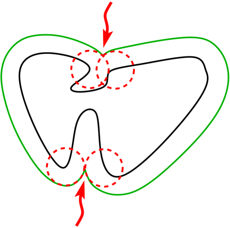
Figure 1: An example in which $G$ is $C^{\infty}$ but $\Omega$ is not $C^{1}$.

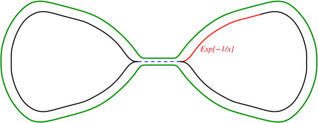
Figure 2: An example in which a parallel set of $\Omega$ is not $C^{1}$ even though $\Omega$ is $C^{\infty}$.

Our main goal is to obtain quantitative bounds on $\rho(\Omega)$ in terms of $[u]_{\partial G}$. In particular, our second main result is the following.

Theorem 1.2.

Let $G$ be an open and bounded set of $\mathbb{R}^{n}$ with $\partial G$ of class $C^{1}$ and let $\Omega:=G+B_{R}$. Assume that $\partial\Omega$ is of class $C^{2}$. Let $u\in C^{2}(\Omega)\cap C(\mathbb{R}^{n})$ be a solution of (1.2). Then, we have that

$$\rho(\Omega)\leq C_{*}\,[u]_{\partial G}^{\frac{1}{s+2}},$$ (1.7)

where $C_{*}>0$ is an explicit constant only depending on $n$, $s$, $R$, and the diameter $\mathrm{diam}(\Omega)$ of $\Omega$.

Hence, Theorem 1.2 asserts that the quantity $[u]_{\partial G}$ bounds from above a pointwise measure of closeness of $\Omega$ to a ball, namely $\rho(\Omega)$. The closer $[u]_{\partial G}$ is to zero, the closer the domain $\Omega$ is to a ball (in a pointwise sense). Of course, when $[u]_{\partial G}=0$, estimate (1.7) reduces to $\rho(\Omega)=0$, and therefore (1.6) gives that $\Omega$ is a ball: in this sense, Theorem 1.2 recovers Theorem 1.1.

We notice that the quantitative estimate (1.7) is of Hölder type and may be not optimal since we do not recover the optimal linear bound at the limit for $s\to 1$ which was obtained in [CMS16]. The main reason for the exponent $\frac{1}{s+2}$ in (1.7) is due to the technique used to obtain our quantitative estimates, which are significantly different from the local case and rely on detecting “useful mass” of the functions involved in suitable regions of the domain.

We stress that the assumption that the constant $C_{*}$ in Theorem 1.2 depends on the diameter of $\Omega$ is essential and cannot be removed: an explicit example will be presented in Section 7.

We finally notice that we do not have to make any assumption on connectedness on $G$. This is a remarkable difference with respect to the classical local case [CMS16]. In this direction it is not difficult to see that Theorems 1.1 and 1.2 hold under weaker assumptions, in particular by assuming that the value $c$ in (1.3) may be different on each connected component of $G$. In Section 8 we give further and more precise details on this result.

This paper is organized as follows. In Section 2 we present a new boundary Harnack result on a half ball for antisymmetric $s$-harmonic functions. Section 3 is devoted to the moving planes method and the proof of Theorem 1.1; we make use of weak and strong maximum principles, as well as the boundary Harnack that we have established in Section 2.

In Section 4 we present a quantitative version of the fractional Hopf lemma introduced in [FJ15, Proposition 3.3]. Section 5 uses the previous results in order to get a quantitative stability estimate in one direction. Lastly, in Section 6 we complete the proof of Theorem 1.2 by passing from the approximate symmetry in one direction to the desired quantitative symmetry result following an idea used in [CFMN18].

Section 7 presents an example that shows that the dependence of the constant $C_{*}$ in Theorem 1.2 upon the diameter of the domain cannot be removed. In Section 8 we describe some possible generalization of Theorems 1.1 and 1.2. A technical observation of geometric type is placed in Appendix A.

In general, we believe that the auxiliary results developed in this article, such as the boundary Harnack estimate for antisymmetric $s$-harmonic functions and the corresponding quantitative version of the fractional Hopf lemma are of independent interest and can be used in other contexts too.

In terms of applications, in addition to the classical motivations in the study of invariant isothermic surfaces [MS10], we mention that the overdetermined problem in (1.2) and (1.3) can be inspired by questions related to population dynamics and specifically to the determination of optimal rural-urban fringes: in this context, our results would detect that the fair shape for an urban settlement is the circular one, as detailed in Appendix B.

2 Boundary Harnack inequality

We present here a new boundary Harnack inequality for antisymmetric $s$-harmonic functions. From now on, we will employ the notation $H^{+}:=\{x_{1}>0\}$, $H^{-}:=\{x_{1}<0\}$ and $T\coloneqq\{x_{1}=0\}$. We define $Q:\mathbb{R}^{n}\to\mathbb{R}^{n}$, with $y\mapsto y^{\prime}=(-y_{1},y_{2},\dots,y_{n})$, the reflection with respect to $T$. Moreover, for $R>0$ we call $B^{+}_{R}:=B_{R}\cap H^{+}$ and $B^{-}_{R}:=B_{R}\cap H^{-}$.

The main result towards the boundary Harnack inequality in our setting is the following:

Lemma 2.1.

Let $u\in C^{2}(B_{R})\cap C(\mathbb{R}^{n})$ with

$$\int_{\mathbb{R}^{n}}\frac{|u(x)|}{1+|x|^{n+2s}}<+\infty$$ (2.1)

be a solution of

$$\begin{cases}(-\Delta)^{s}u=0\quad&\text{in }B_{R},\\ u(x^{\prime})=-u(x)\quad&\text{for every }x\in\mathbb{R}^{n},\\ u\geq 0\quad&\text{in }H^{+}.\end{cases}$$

There exists a constant $K>1$ only depending on $n$ and $s$ such that, for every $z\in B_{R/2}^{+}$ and for every $x\in B_{R/4}(z)\cap B_{R}^{+}$ we have

$$\frac{1}{K}\frac{u(z)}{z_{1}}\leq\frac{u(x)}{x_{1}}\leq K\frac{u(z)}{z_{1}}.$$ (2.2)

Proof.

We recall that the Poisson Kernel for the fractional Laplacian in the ball is given by (see for example [Buc16])

$$P_{n,s}(x,y)\coloneqq c_{n,s}\bigg{(}\frac{R^{2}-|x|^{2}}{|y|^{2}-R^{2}}\bigg{)}^{s}\frac{1}{|x-y|^{n}}.$$

Hence for every $x\in B_{R}$, we have

$$\begin{split}\frac{u(x)}{c_{n,s}}\,=\,&\int_{\mathbb{R}^{n}\setminus B_{R}(0)}\bigg{(}\frac{R^{2}-|x|^{2}}{|y|^{2}-R^{2}}\bigg{)}^{s}\frac{1}{|x-y|^{n}}u(y)\,dy\\ =\,&\int_{H^{+}\setminus B_{R}^{+}}\bigg{(}\frac{R^{2}-|x|^{2}}{|y|^{2}-R^{2}}\bigg{)}^{s}\frac{1}{|x-y|^{n}}u(y)\,dy-\int_{H^{+}\setminus B_{R}^{+}}\bigg{(}\frac{R^{2}-|x|^{2}}{|y|^{2}-R^{2}}\bigg{)}^{s}\frac{1}{|x-y^{\prime}|^{n}}u(y)\,dy\\ =\,&\int_{H^{+}\setminus B_{R}^{+}}\bigg{(}\frac{R^{2}-|x|^{2}}{|y|^{2}-R^{2}}\bigg{)}^{s}\bigg{(}\frac{1}{|x-y|^{n}}-\frac{1}{|x-y^{\prime}|^{n}}\bigg{)}u(y)\,dy=:\int_{H^{+}\setminus B_{R}^{+}}\frac{T_{n,s}(x,y)}{c_{n,s}}u(y)dy.\end{split}$$

Our goal is to show that there exists a constant $K>1$ depending only on $n$ and $s$ such that

$$\frac{1}{K}\,\frac{x_{1}}{z_{1}}\leq\frac{T_{n,s}(x,y)}{T_{n,s}(z,y)}\leq K\,\frac{x_{1}}{z_{1}},$$ (2.3)

for every $z\in B_{R/2}^{+}$, $x\in B_{R/4}(z)\cap B_{R}^{+}$ and $y\in H^{+}\setminus B_{R}^{+}$.

We remark that once (2.3) is established the claim in (2.2) readily follows, since

$$\frac{u(x)}{x_{1}}=\int_{H^{+}\setminus B_{R}^{+}}\frac{T_{n,s}(x,y)}{x_{1}}u(y)dy\leq K\int_{H^{+}\setminus B_{R}^{+}}\frac{T_{n,s}(z,y)}{z_{1}}u(y)dy=K\,\frac{u(z)}{z_{1}},$$

which is precisely the second inequality in (2.2). The first inequality in (2.2) can be obtained similarly.

Now we prove (2.3). We notice that

$$\begin{split}\frac{T_{n,s}(x,y)}{T_{n,s}(z,y)}\,=&\,\bigg{(}\frac{R^{2}-|x|^{2}}{|y|^{2}-R^{2}}\bigg{)}^{s}\,\bigg{(}\frac{|y|^{2}-R^{2}}{R^{2}-|z|^{2}}\bigg{)}^{s}\,\bigg{(}\frac{1}{|x-y|^{n}}-\frac{1}{|x-y^{\prime}|^{n}}\bigg{)}\bigg{(}\frac{1}{|z-y|^{n}}-\frac{1}{|z-y^{\prime}|^{n}}\bigg{)}^{-1}\\ =\,&\bigg{(}\frac{R^{2}-|x|^{2}}{R^{2}-|z|^{2}}\bigg{)}^{s}\,\frac{|z-y|^{n}}{|x-y|^{n}}\,\frac{|z-y^{\prime}|^{n}}{|x-y^{\prime}|^{n}}\,\frac{|x-y^{\prime}|^{n}-|x-y|^{n}}{|z-y^{\prime}|^{n}-|z-y|^{n}}\,,\end{split}$$ (2.4)

and we estimate the first term as follows

$$\bigg{(}\frac{7}{16}\bigg{)}^{s}\leq\bigg{(}\frac{R^{2}-(3R/4)^{2}}{R^{2}}\bigg{)}^{s}\leq\bigg{(}\frac{R^{2}-|x|^{2}}{R^{2}-|z|^{2}}\bigg{)}^{s}\leq\bigg{(}\frac{R^{2}}{R^{2}-(R/2)^{2}}\bigg{)}^{s}\leq\bigg{(}\frac{4}{3}\bigg{)}^{s}.$$ (2.5)

Moreover, we observe that

$$\begin{split}&\frac{|z-y|}{|x-y|}\leq\frac{|x-y|}{|x-y|}+\frac{|x-z|}{|x-y|}\leq 1+\frac{R/4}{R/4}=2,\\ &\frac{|z-y|}{|x-y|}\geq\frac{|y|-|z|}{|y|+|x|}\geq\frac{|y|-R/2}{|y|+3R/4}\geq\frac{2}{7}.\end{split}$$ (2.6)

Now, considering the last terms in (2.4), we can write

$$\frac{|z-y^{\prime}|^{n}}{|x-y^{\prime}|^{n}}\,\frac{|x-y^{\prime}|^{n}-|x-y|^{n}}{|z-y^{\prime}|^{n}-|z-y|^{n}}=:\frac{1-\alpha^{n}}{1-\beta^{n}}\,,$$ (2.7)

where

$$\alpha=\frac{|x-y|}{|x-y^{\prime}|}\quad\text{ and }\quad\beta=\frac{|z-y|}{|z-y^{\prime}|}\,.$$

We observe that

$$0\leq\alpha^{2}=\frac{|x-y|^{2}}{|x-y^{\prime}|^{2}}=1-\frac{4x_{1}y_{1}}{|x-y^{\prime}|^{2}}\leq 1\quad\text{and}\quad 0\leq\beta^{2}=\frac{|z-y|^{2}}{|z-y^{\prime}|^{2}}=1-\frac{4z_{1}y_{1}}{|z-y^{\prime}|^{2}}\leq 1\,.$$ (2.8)

Going back to (2.7) we write

$$\frac{1-\alpha^{n}}{1-\beta^{n}}\,=\frac{(1-\alpha)(1+\alpha+\dots+\alpha^{n-1})}{(1-\beta)(1+\beta+\dots+\beta^{n-1})}\,=\left[\frac{1-\alpha^{2}}{1-\beta^{2}}\right]\frac{(1+\beta)(1+\alpha+\dots+\alpha^{n-1})}{(1+\alpha)(1+\beta+\dots+\beta^{n-1})}.$$

From (2.8) we easily get

$$\frac{1}{2n}\leq\frac{(1+\beta)(1+\alpha+\dots+\alpha^{n-1})}{(1+\alpha)(1+\beta+\dots+\beta^{n-1})}\leq 2n$$ (2.9)

and, using estimates similar to the ones in (2.6),

$$\bigg{(}\frac{2}{7}\bigg{)}^{2}\,\frac{x_{1}}{z_{1}}\leq\frac{1-\alpha^{2}}{1-\beta^{2}}\leq 4\,\frac{x_{1}}{z_{1}}.$$ (2.10)

By plugging (2.9) and (2.10) into equation (2.7) and then combining it with (2.5) and (2.6), from (2.4) we get

$$\bigg{(}\frac{7}{16}\bigg{)}^{s}\,\bigg{(}\frac{2}{7}\bigg{)}^{n}\,\frac{1}{2n}\,\frac{x_{1}}{z_{1}}\leq\frac{T_{n,s}(x,y)}{T_{n,s}(z,y)}\leq\bigg{(}\frac{4}{3}\bigg{)}^{s}\,2^{n+3}\,n\,\frac{x_{1}}{z_{1}}$$

which leads to (2.3) if we set $K=K(n,s):=(4/3)^{s}(7/2)^{n+2}\,2n>1$. This completes the proof. ∎

As a consequence of the previous result, we get the following two propositions which provide boundary Harnack’s inequalities of independent interest:

Proposition 2.2.

Let $u\in C^{2}(B_{R})\cap C(\mathbb{R}^{n})$ be antisymmetric w.r.t. $T$, $s$-harmonic in $B_{R}$, nonnegative in $H^{+}$ and such that (2.1) holds. Then,

$$\sup_{B_{R/2}^{+}}u\leq Mu(\hat{x}),$$ (2.11)

where $\hat{x}=\frac{R}{2}e_{1}$ and $M>0$ is a constant depending on $n$ and $s$.

Proof.

Let $x_{\star}\in\overline{B_{R/2}^{+}}$ be such that

$$u(x_{\star})=\sup_{B_{R/2}^{+}}u.$$

If $u(x_{\star})=0$ the result is trivial. Therefore, we can assume $u(x_{\star})>0$ and $(x_{\star})_{1}>0$.

We now point out that any point $x\in B_{R/2}^{+}$ can be connected to $\hat{x}$ by a Harnack chain made at most of $3$ balls of radius $R/4$. Hence, by choosing $x_{a},\,x_{b}\in B_{R/2}^{+}$ such that

$$\mathrm{dist}(x_{\star},x_{a})\leq R/4,\quad\mathrm{dist}(x_{a},x_{b})\leq R/4\quad and\quad\mathrm{dist}(x_{b},x_{\star})\leq R/4$$

we can then apply Lemma 2.1 and get

$$\frac{1}{K}\,\frac{u(x_{\star})}{(x_{\star})_{1}}\leq\frac{u(x_{a})}{(x_{a})_{1}}\leq K\,\frac{u(x_{b})}{(x_{b})_{1}}\leq K^{2}\,\frac{u(\hat{x})}{(\hat{x})_{1}}$$

which gives

$$\sup_{B_{R/2}^{+}}u=u(x_{\star})\leq K^{3}\,\frac{u(\hat{x})}{R/2}\,(x_{\star})_{1}\leq K^{3}\,u(\hat{x}),$$

where in the last inequality we have used that $(x_{\star})_{1}\leq R/2$. ∎

Proposition 2.3.

Let $u,v\in C^{2}(B_{R})\cap C(\mathbb{R}^{n})$ be antisymmetric w.r.t. $T$ and satisfying (2.1), and assume that

$$\begin{cases}(-\Delta)^{s}u=0=(-\Delta)^{s}v\quad in\ B_{R}^{+},\\ u,v\geq 0\quad in\ H^{+}.\end{cases}$$ (2.12)

Then

$$\sup_{B_{R/2}^{+}}\frac{u}{v}\leq K^{2}\inf_{B_{R/2}^{+}}\frac{u}{v},$$ (2.13)

where $K=K(n,s)>1$ is the constant given in (2.2).

Proof.

From Lemma 2.1 we have that for every $z\in B_{R/2}^{+}$ and every $x\in B_{R/4}(z)\cap B_{R}^{+}$

$$\frac{1}{K^{2}}\frac{u(z)}{v(z)}\leq\frac{u(x)}{v(x)}\leq K^{2}\frac{u(z)}{v(z)}.$$

The proof then follows by using the Harnack chain as done in the proof of Proposition 2.2. ∎

3 Moving planes method and symmetry result

We introduce the notation needed in order to exploit the moving planes method. Given $e\in\mathbb{S}^{n-1}$, a set $E\subset\mathbb{R}^{n}$ and $\lambda\in\mathbb{R}$, we set

$$T_{\lambda}=T_{\lambda}^{e}=\{x\in\mathbb{R}^{n}\,|\,x\cdot e=\lambda\} \textrm{a hyperplane orthogonal to }e,$$

$$H_{\lambda}=H_{\lambda}^{e}=\{x\in\mathbb{R}^{n}\,|\,x\cdot e>\lambda\} \textrm{the ``positive'' half space with respect to }T_{\lambda}$$

$$E_{\lambda}=E\cap H_{\lambda} \textrm{the ``positive'' cap of }E,$$

$$x_{\lambda}^{\prime}=x-2(x\cdot e-\lambda)\,e \textrm{the reflection of }x\textrm{ with respect to }T_{\lambda},$$

$$Q=Q_{\lambda}^{e}:\mathbb{R}^{n}\to\mathbb{R}^{n},x\mapsto x_{\lambda}^{\prime} \textrm{the reflection with respect to }T_{\lambda}.$$

If $E\subset\mathbb{R}^{n}$ is an open bounded set with boundary of class $C^{1}$ and $\Lambda_{e}:=\sup\{x\cdot e\,|\,x\in E\}$ it makes sense to define

$$\lambda_{e}=\inf\{\lambda\in\mathbb{R}\,|\,Q(E_{\tilde{\lambda}})\subset E,\textrm{for all}\,\tilde{\lambda}\in(\lambda,\Lambda_{e})\}.$$

From this point on, given a direction $e\in\mathbb{S}^{n-1}$, we will refer to $T_{\lambda_{e}}=T^{e}$ and $E_{\lambda_{e}}=\widehat{E}$ as the critical hyperplane and the critical cap with respect to $e$, respectively, and we call $\lambda_{e}$ the critical value in the direction $e$. We now recall from [Ser71] that for any given direction $e$ one of the following two conditions holds:

Case 1 - The boundary of the cap reflection $Q^{e}(\widehat{E})$ becomes internally tangent to the boundary of $E$ at some point $P\not\in T^{e}$;

Case 2 - the critical hyperplane $T^{e}$ becomes orthogonal to the boundary of $E$ at some point $Q\in T^{e}$.

Throughout this paper, the method of moving planes will be applied to the set $E=G$, where $G$ is the set appearing in (1.1). Hence the minimal regularity assumption that we need on $G$ is that $G$ is of class $C^{1}$. We also notice that, in our setting, the critical values $\lambda_{e}$ for $G$ are also critical values for the set $\Omega$, even if we do not need to assume further regularity on $\Omega$ in order to apply the method of moving planes. This is the reason why in Theorem 1.1 we only require that $G$ is of class $C^{1}$. We also notice that in Theorem 1.2 we assume that $\Omega$ is of class $C^{2}$, but this assumption is not needed for the application of the method of moving planes but it comes from using other tools in the proof.

In order to prove symmetry for the problem (1.2) with condition (1.3) we will use a fractional version of the weak and strong maximum principles and a Hopf-type Lemma for antisymmetric $s$-harmonic functions.

For $u,v\in H^{s}(\mathbb{R}^{n})$, we consider the bilinear form induced by the fractional Laplacian

$$\mathcal{E}(u,v):=\frac{c_{n,s}}{2}\int_{\mathbb{R}^{n}}\int_{\mathbb{R}^{n}}\frac{\big{(}u(x)-u(y)\big{)}\big{(}v(x)-v(y)\big{)}}{|x-y|^{n+2s}}dxdy.$$

Let

$$\mathcal{D}^{s}(\Omega):=\{u:\mathbb{R}^{n}\to\mathbb{R}\quad\mathrm{measurable}\ :\ \mathcal{E}(u,\varphi)\text{ is finite in Lebesgue sense for every }\varphi\in H^{s}_{0}(\Omega)\}\,,$$

where

$$H^{s}_{0}(\Omega):=\{u\in H^{s}(\mathbb{R}^{n})\ :\ u=0\ \text{ on }\mathbb{R}^{n}\setminus\Omega\}.$$

See e.g. [DNPV12b, Gri11] and the references therein for further information about fractional functional spaces.

Given $g\in L^{2}(\Omega)$ we say that a function $u\in\mathcal{D}^{s}(\Omega)$ is a solution of

$$\begin{cases}(-\Delta)^{s}u=g\quad&in\ \Omega,\\ u=0\quad&in\ \mathbb{R}^{n}\setminus\Omega,\end{cases}$$ (3.1)

if for all $\varphi\in H_{0}^{s}(\Omega)$ we have

$$\mathcal{E}(u,\varphi)=\int_{\Omega}g(x)\,\varphi(x)\,dx.$$

It will be useful to introduce the notion of entire antisymmetric supersolution. Let $H\subset\mathbb{R}^{n}$ be a half space and let $A$ be an open set with $A\subset H$. Given $\tilde{g}\in L^{2}(A)$ we say that $v\in\mathcal{D}^{s}(A)$ is an entire antisymmetric supersolution of $(-\Delta)^{s}v=\tilde{g}$ in $A$, if the following conditions hold:

• $v$ is a supersolution of $(-\Delta)^{s}v=\tilde{g}$ in $A$, that is, for all $\varphi\in H_{0}^{s}(A)$, $\varphi\geq 0$ we have

  $$\mathcal{E}(v,\varphi)\geq\int_{A}\tilde{g}(x)\,\varphi(x)\,dx,$$

• $v\geq 0$ in $H\setminus A$ and $v$ is antisymmetric with respect to $\partial H$.

We are now ready to prove Theorem 1.1.

Proof of Theorem 1.1.

We apply the method of moving planes to the set $G$. Let $e\in\mathbb{S}^{n-1}$ be a fixed direction. Without loss of generality, we can assume that $e=e_{1}$ and that the critical hyperplane $T$ goes through the origin (that is, $\lambda_{e}=0$). We call $H^{-}:=\{x_{1}<0\}$ and consider the function

$$v(x):=u(x)-u(Q(x))\quad\mathrm{for}\ x\in\mathbb{R}^{n},$$

where $Q:\mathbb{R}^{n}\to\mathbb{R}^{n}$ is the reflection with respect to $T$. We have

$$\begin{cases}(-\Delta)^{s}v=0\quad&in\ Q(\widehat{\Omega}),\\ v\geq 0\quad&in\ H^{-}\setminus Q(\widehat{\Omega}),\\ v(Q(x))=-v(x)\quad&\mathrm{for\ every}\ x\in\mathbb{R}^{n}.\end{cases}$$

Thus, $v$ is an entire antisymmetric supersolution on $Q(\widehat{\Omega})$. By the weak maximum principle (see [FJ15, Proposition 3.1]) we know that $v\geq 0$ in $H^{-}$. The strong maximum principle (see [FJ15, Corollary 3.4]) then implies that either $v>0$ in $Q(\widehat{\Omega})$ or $v\equiv 0$ in $\mathbb{R}^{n}$. We will show that the first possibility cannot occur.

Assume by contradiction that $v>0$ in $Q(\widehat{\Omega})$. We need to distinguish between the two possible critical cases.

Case 1 - since both $P$ and $P^{\prime}$ belong to $\partial G$ and (1.3) holds, we immediately get that

$$v(P)=u(P)-u(P^{\prime})=0,$$

which is already a contradiction.

Case 2 - in this case the critical hyperplane $T=\{x_{1}=0\}$ is orthogonal to $\partial G$ at some point $Q=(0,Q_{2},\dots,Q_{n})$ and therefore (1.3) ensures that

$$\partial_{1}v(Q)=0.$$ (3.2)

On the other hand, Lemma 2.1 implies the following Hopf-type inequality

$$\partial_{1}v(Q)<0,$$ (3.3)

which contradicts (3.2) and hence (1.3). Indeed, setting $z=(-R/4,Q_{2},\dots,Q_{n})$ and $x=x_{t}=(-t,Q_{2},\dots,Q_{n})\in B_{R/4}(z)$, we have that

$$\frac{v(x_{t})}{-t}\geq-\frac{4}{RK}v(z),$$ (3.4)

where $K>1$ is a constant only depending on $n$ and $s$. Being $z\in Q(\widehat{\Omega})$, we have that $v(z)>0$, and by letting $t$ go to 0 (3.3) follows by (3.4).

This implies that $G$ (and hence $\Omega$) is symmetric with respect to the direction $e$. Since the direction $e$ is arbitrary, we easily obtain that $G$ (and hence $\Omega$) is a ball. ∎

An alternative approach to the Hopf-type inequality (3.3) will be developed in a forthcoming manuscript [DPTV22].

4 A quantitative maximum principle

The following lemma is a quantitative version of [FJ15, Proposition 3.3]. To state it, we adopt the notion of distance between two sets, say $X$ and $Y$, defined by

$$\mathrm{dist}(X,Y):=\inf\big{\{}|x-y|,\quad x\in X,\;y\in Y\big{\}}.$$

Lemma 4.1.

Let $B\subset H^{-}$ be a ball of radius $R>0$ such that $\mathrm{dist}(B,H^{+})>0$. Let $v\in C^{s}(B)$ be an entire antisymmetric supersolution of

$$\begin{cases}(-\Delta)^{s}v=0\quad&in\ B,\\ v\geq 0\quad&in\ H^{-}.\end{cases}$$

Let $K\subset H^{-}$ be a bounded set of positive measure such that $\overline{K}\subset(H^{-}\setminus\overline{B})$ and $\inf_{K}v>0$. Then we have that

$$v\geq C\Big{[}\mathrm{dist}(K,H^{+})\,|K|\,\inf_{K}v\Big{]}\psi_{B}\quad in\ B,$$ (4.1)

where $\psi_{B}$ is defined in (1.4), with

$$C:=\frac{2(n+2s)\,C(n,s)\,\mathrm{dist}(B,H^{+})^{n+2s+1}}{\big{(}\mathrm{dist}(B,H^{+})^{n+2s}+C(n,s)\,|B|\,\gamma_{n,s}\,R^{2s}\big{)}\big{(}\mathrm{diam}(B)+\mathrm{diam}(K)+\mathrm{dist}(Q(K),B)\big{)}^{n+2s+2}}.$$

Proof.

We define

$$w(x):=\psi_{B}(x)-\psi_{Q(B)}(x)+\alpha\mathbbm{1}_{K}(x)-\alpha\mathbbm{1}_{Q(K)}(x)\quad\textrm{for }\ x\in\mathbb{R}^{n}$$

where $\alpha>0$ is a parameter to be set later on, $\psi_{B}$ is the solution of the fractional torsion problem in $B$ and $\mathbbm{1}_{A}$ is the characteristic function of a given set $A$. A direct computation shows that $w\in\mathcal{D}^{s}(B)$.

The function $w$ is antisymmetric and for any nonnegative test function $\varphi\in H_{0}^{s}(B)$ we have

$$\mathcal{E}(w,\varphi) =\mathcal{E}(\psi_{B},\varphi)-\mathcal{E}(\psi_{Q(B)},\varphi)+\alpha\,\mathcal{E}(\mathbbm{1}_{K},\varphi)-\alpha\,\mathcal{E}(\mathbbm{1}_{Q(K)},\varphi)$$

$$=\int_{B}\varphi(x)dx+C(n,s)\int_{B}\int_{Q(B)}\frac{\psi_{Q(B)}(y)\varphi(x)}{|x-y|^{n+2s}}dydx$$

$$-\alpha\ C(n,s)\int_{B}\int_{K}\frac{\varphi(x)}{|x-y|^{n+2s}}dydx+\alpha\ C(n,s)\int_{B}\int_{Q(K)}\frac{\varphi(x)}{|x-y|^{n+2s}}dydx$$

$$\leq\int_{B}\varphi(x)dx\bigg{[}\kappa-\alpha\ C(n,s)\int_{K}\bigg{(}\frac{1}{|x-y|^{n+2s}}-\frac{1}{|x-y^{\prime}|^{n+2s}}\bigg{)}\bigg{]},$$

where

$$\kappa=\kappa(n,s,B)=1+C(n,s)\,|B|\sup_{B}\psi_{B}\sup_{x\in B,y\in H^{+}}\frac{1}{|x-y|^{n+2s}}<+\infty.$$

If we set

$$C_{1}=C_{1}(n,s,K,B)=C(n,s)\ |K|\ \inf_{x\in B,y\in K}\bigg{(}\frac{1}{|x-y|^{n+2s}}-\frac{1}{|x-y^{\prime}|^{n+2s}}\bigg{)}>0,$$ (4.2)

then

$$\mathcal{E}(w,\varphi)\leq\int_{B}\varphi(x)(\kappa-\alpha C_{1}).$$

By choosing $\alpha$ in such a way that $\kappa-\alpha C_{1}\leq 0$, we get $(-\Delta)^{s}w\leq 0$ in $B$.

For concreteness, we can thus choose

$$\alpha:=\frac{\kappa}{C_{1}}$$

to have the previous argument in place and then set

$$\tau\coloneqq\inf_{K}\frac{v}{\alpha}>0$$

and define

$$\tilde{v}(x)\coloneqq v(x)-\tau w(x)$$

for every $x\in\mathbb{R}^{n}$. Recalling that $w$ is antisymmetric and that $w\equiv 0$ on $H^{-}\setminus(B\cup K)$ we have

$$\begin{cases}(-\Delta)^{s}\tilde{v}\geq 0\quad&\text{in }B\\ \tilde{v}\geq 0\quad&\text{in }H^{-}\setminus B.\end{cases}$$

From the weak maximum principle we then get that $\tilde{v}\geq 0$ in $B$ and, in particular,

$$v\geq\tau\psi_{B}\quad\text{in }B.$$ (4.3)

For every $x\in B$ and every $y\in K$ we compute

$$\begin{split}\frac{1}{|x-y|^{n+2s}}-\frac{1}{|x-y^{\prime}|^{n+2s}}&=\frac{n+2s}{2}\int_{|x-y|^{2}}^{|x-y^{\prime}|^{2}}t^{-\frac{n+2s+2}{2}}dt\\ &\geq\frac{n+2s}{2}\big{(}|x-y^{\prime}|^{2}-|x-y|^{2}\big{)}|x-y^{\prime}|^{-(n+2s+2)}\\ &\geq\frac{n+2s}{2}4x_{1}y_{1}|x-y^{\prime}|^{-(n+2s+2)}.\end{split}$$

Moreover, for all $x\in B$ and $y\in K$,

$$|x-y^{\prime}|\leq\mathrm{diam}(B)+\mathrm{diam}(K)+\mathrm{dist}(Q(K),B)$$

and consequently

$$\frac{1}{|x-y|^{n+2s}}-\frac{1}{|x-y^{\prime}|^{n+2s}}\geq\frac{2(n+2s)\mathrm{dist}(B,H^{+})\,\mathrm{dist}(K,H^{+})}{\big{(}\mathrm{diam}(B)+\mathrm{diam}(K)+\mathrm{dist}(Q(K),B)\big{)}^{n+2s+2}}.$$

Hence, by (4.2),

$$C_{1}\geq\frac{2(n+2s)\,C(n,s)\,|K|\,\mathrm{dist}(B,H^{+})\,\mathrm{dist}(K,H^{+})}{\big{(}\mathrm{diam}(B)+\mathrm{diam}(K)+\mathrm{dist}(Q(K),B)\big{)}^{n+2s+2}.}$$

As a result,

$$\tau=\frac{C_{1}}{\kappa}\inf_{K}v\geq\frac{2(n+2s)\,C(n,s)\,|K|\,\mathrm{dist}(B,H^{+})\,\mathrm{dist}(K,H^{+})}{\kappa\,\big{(}\mathrm{diam}(B)+\mathrm{diam}(K)+\mathrm{dist}(Q(K),B)\big{)}^{n+2s+2}}\inf_{K}v.$$

We also observe, owing to (1.4), that

$$\sup_{B}\psi_{B}(x)=\gamma_{n,s}\,R^{2s}$$

and therefore

$$\kappa = 1+C(n,s)\,|B|\,\gamma_{n,s}\,R^{2s}\,\sup_{x\in B,y\in H^{+}}\frac{1}{|x-y|^{n+2s}}$$

$$\leq 1+\frac{C(n,s)\,|B|\,\gamma_{n,s}\,R^{2s}}{\mathrm{dist}(B,H^{+})^{n+2s}}$$

$$= \frac{\mathrm{dist}(B,H^{+})^{n+2s}+C(n,s)\,|B|\,\gamma_{n,s}\,R^{2s}}{\mathrm{dist}(B,H^{+})^{n+2s}}.$$

Accordingly,

$$\tau\geq\frac{2(n+2s)\,C(n,s)\,|K|\,\mathrm{dist}(B,H^{+})^{n+2s+1}\,\mathrm{dist}(K,H^{+})}{\big{(}\mathrm{dist}(B,H^{+})^{n+2s}+C(n,s)\,|B|\,\gamma_{n,s}\,R^{2s}\big{)}\big{(}\mathrm{diam}(B)+\mathrm{diam}(K)+\mathrm{dist}(Q(K),B)\big{)}^{n+2s+2}}\inf_{K}v.$$

Thus, the desired conclusion follows from (4.3). ∎

5 Almost symmetry in one direction

As customary, we say that a bounded domain $\Omega\subset\mathbb{R}^{n}$ satisfies the uniform interior ball condition if there exists a radius $r_{\Omega}>0$ such that for every point $x_{0}\in\partial\Omega$ we can find a ball $B_{i}\subset\Omega$ of radius $r_{\Omega}$ with $\overline{B_{i}}\cap\Omega^{c}=\{x_{0}\}$.

In the next subsection, we collect some useful technical lemmas which hold true for domains satisfying such a condition.

5.1 Preliminaries: some results for domains satisfying the uniform interior ball condition

As noticed in [CPY22, MP23], the following simple explicit bound for the perimeter holds true.

Lemma 5.1 (A general simple upper bound for the perimeter, [CPY22, MP23]).

Let $D\subset\mathbb{R}^{n}$ be a bounded domain with boundary of class $C^{1,\alpha}$, with $0<\alpha\leq 1$. If $D$ satisfies the uniform interior ball condition with radius $r_{D}$, the we have that

$$|\partial D|\leq\frac{n|D|}{r_{D}}.$$ (5.1)

Proof.

By following [MP23], the desired bound can be easily obtained by considering the solution $f\in C^{1,\alpha}(\overline{D})$ to

$$\Delta f=n\,\text{ in }D,\quad f=0\,\text{ on }\partial D,$$

and putting together the identity

$$n|D|=\int_{\partial D}\partial_{\nu}f\,d\mathcal{H}^{n-1},\text{ where }\partial_{\nu}\text{ denotes the outer normal derivative},$$

with the Hopf-type inequality

$$\partial_{\nu}f\geq r_{D},$$

which can be found in [MP19, Theorem 3.10].

We mention that a more general version of the bound (5.1) remains true even without assuming the uniform interior ball condition, at the cost of replacing the radius $r_{D}$ of the ball condition with a parameter associated to the (weaker) pseudoball condition, which is always verified by $C^{1,\alpha}$ domains: see [CPY22, Remark 1.1] and the last displayed inequality in the proof of [CPY22, Corollary 2.1]. ∎

The previous result is useful to prove the following.

Lemma 5.2.

Let $\Omega\subset\mathbb{R}^{n}$ be a bounded domain with $\partial\Omega$ of class $C^{2}$. For $\delta>0$, we set

$$A_{\delta}:=\{x\in\Omega\ |\ \mathrm{dist}(x,\partial\Omega)<\delta\}.$$ (5.2)

Then, we have that

$$|A_{\delta}|\leq c\,\delta,\quad\text{ with }\quad c:=\frac{2n|\Omega|}{r_{\Omega}},$$ (5.3)

where $r_{\Omega}$ is the radius of the uniform interior ball condition of $\Omega$.

We recall that if a domain has boundary of class $C^{2}$, then it satisfies a uniform interior ball condition.

Proof of Lemma 5.2.

We set $d_{\partial\Omega}(x):=\mathrm{dist}(x,\partial\Omega)$ for $x\in\Omega$. For $\delta\geq 0$, we define

$$V_{\delta}:=\{x\in\Omega\ |\ d_{\partial\Omega}(x)>\delta\}\quad\text{ and }\quad\Gamma_{\delta}:=\{x\in\Omega\ |\ d_{\partial\Omega}(x)=\delta\}\,.$$

It is well-known that $d_{\partial\Omega}\in C^{2}(A_{r_{\Omega}})$ (see, e.g., [GT77, Lemma 14.16]).

We first prove the claim in the case $0\leq\delta\leq r_{\Omega}/2$. From the coarea formula we obtain

$$|A_{\delta}|=\int_{A_{\delta}}1\,dx=\int_{A_{\delta}}|\nabla d_{\partial\Omega}(x)|\,dx=\int_{0}^{\delta}\bigg{(}\int_{A_{\delta}\cap d_{\partial\Omega}^{-1}(t)}d\mathcal{H}^{n-1}\bigg{)}\,dt=\int_{0}^{\delta}|\Gamma_{t}|\,dt.$$ (5.4)

Since $t\leq\delta\leq r_{\Omega}/2$, we have that $V_{t}$ is a bounded domain satisfying the uniform interior touching ball condition with radius $r_{\Omega}/2$, and with boundary $\Gamma_{t}$ of class $C^{2}$. Thus, we can apply Lemma 5.1 with $D:=V_{t}$ to get that

$$|\Gamma_{t}|\leq\frac{2n|V_{t}|}{r_{\Omega}}\leq\frac{2n|\Omega|}{r_{\Omega}},$$ (5.5)

where the last inequality follows by the inclusion $V_{t}\subseteq\Omega$. Combining (5.4) with (5.5) immediately gives (5.3), for any $0\leq\delta\leq r_{\Omega}/2$.

On the other hand, if $\delta\geq r_{\Omega}/2$, we easily find that

$$|A_{\delta}|\leq|\Omega|\leq\left[\frac{2|\Omega|}{r_{\Omega}}\right]\delta,$$

where the first inequality follows by the inclusion

$$A_{\delta}\subseteq\Omega,\text{ for any }\delta\geq 0.$$

Thus, (5.3) still holds true. ∎

We now detect an optimal growth of the solution to (1.2) from the boundary, by generalizing [MP20, Lemma 3.1] to the fractional setting.

Lemma 5.3.

Let $u$ satisfy (1.2) and let $\gamma_{n,s}$ be the constant defined in (1.5). Then,

$$u(x)\geq\gamma_{n,s}\,\mathrm{dist}(x,\partial\Omega)^{2s}\quad\mbox{ for every }\ x\in\Omega.$$ (5.6)

Moreover, if $\Omega$ is of class $C^{1}$ and satisfies the uniform interior sphere condition with radius $r_{\Omega}$, then it holds that

$$u(x)\geq\gamma_{n,s}\,r_{\Omega}^{s}\,\mathrm{dist}(x,\partial\Omega)^{s}\quad\mbox{ for every }\ x\in\Omega.$$ (5.7)

Proof.

Let $x\in\Omega$ and set $r:=\mathrm{dist}(x,\partial\Omega)$. We consider

$$\psi(y):=\gamma_{n,s}\left(r^{2}-|y-x|^{2}\right)_{+}^{s},$$

which satisfies the fractional torsion problem in $B_{r}(x)$, namely

$$\begin{cases}(-\Delta)^{s}\psi=1\quad&\text{ in }B_{r}(x),\\ \psi=0\quad&\text{ on }\mathbb{R}^{n}\setminus B_{r}(x).\end{cases}$$ (5.8)

By the comparison principle (see [FJ15, Remark 3.2]), we have that $u\geq\psi$ on $\overline{B_{r}(x)}$. In particular, at the center $x$ of $B_{r}(x)$, we have that

$$u(x)\geq\psi(x)=\gamma_{n,s}\,\mathrm{dist}(x,\partial\Omega)^{2s},$$

and (5.6) follows.

Notice that (5.7) follows from (5.6) if $\mathrm{dist}(x,\partial\Omega)\geq r_{\Omega}$. Hence, from now on, we can suppose that

$$\mathrm{dist}(x,\partial\Omega)<r_{\Omega}.$$ (5.9)

Let $\bar{x}$ be the closest point in $\partial\Omega$ to $x$ and call $\tilde{B}\subset\Omega$ the ball of radius $r_{\Omega}$ touching $\partial\Omega$ at $\bar{x}$ and containing $x$. Up to a translation, we can always suppose that

the center of the ball $$\tilde{B}$$ is the origin. (5.10)

Now, we let $\tilde{\psi}$ be the solution of (5.8) in $\tilde{B}$, that is $\tilde{\psi}(y):=\gamma_{n,s}\left(r_{\Omega}^{2}-|y|^{2}\right)_{+}^{s}$. By comparison ([FJ15, Remark 3.2]), we have that $u\geq\tilde{\psi}$ in $\tilde{B}$, and hence, being $x\in\tilde{B}$,

$$u(x)\geq\gamma_{n,s}\,(r_{\Omega}^{2}-|x|^{2})_{+}^{s}=\gamma_{n,s}\,(r_{\Omega}+|x|)^{s}(r_{\Omega}-|x|)_{+}^{s}\geq\gamma_{n,s}\,r_{\Omega}^{s}\,(r_{\Omega}-|x|)^{s}.$$ (5.11)

Moreover, from (5.10),

$$r_{\Omega}-|x|=\mathrm{dist}(x,\partial\Omega).$$

This and (5.11) give (5.7), as desired. ∎

5.2 Almost symmetry in one direction

From now on, we let $\Omega\coloneqq G+B_{R}(0)$, with $G\subseteq\mathbb{R}^{n}$ bounded, with $\partial G$ of class $C^{1}$ and $\partial\Omega$ of class $C^{2}$.

Remark 5.4 (On the constants in the quantitative estimates).

The constants in all of our quantitative estimates can be explicitly computed and only depend on $n$, $s$, $R$, and $\mathrm{diam}(\Omega)$. In some of the intermediate results, the parameter $|\Omega|$ may appear. It is clear that such a parameter can be removed thanks to the bounds

$$\frac{\omega_{n}}{n}R^{n}\leq|\Omega|\leq\frac{\omega_{n}}{n}\mathrm{diam}(\Omega)^{n},\text{ where }\frac{\omega_{n}}{n}\text{ is the volume of the unit ball in }\mathbb{R}^{n},$$ (5.12)

which easily hold true in light of the monotonicity of the volume with respect to inclusion.

We remark that the estimates of the previous subsection also depend on the radius $r_{\Omega}$ of the uniform interior ball condition associated to $\Omega$. Nevertheless, from now on, we have that

$$r_{\Omega}:=R,$$ (5.13)

by the definition of $\Omega\coloneqq G+B_{R}(0)$

We apply the method of moving planes to the set $G$. Hence, we fix a direction $e=e_{1}$ and assume the associated critical hyperplane to be $T=\{x_{1}=0\}$, with $Q:\mathbb{R}^{n}\to\mathbb{R}^{n},x\mapsto x^{\prime}$ the reflection with respect to $T$. For the proofs of the next two lemmas we will use the following notation: we set for $t\geq 0$

$$G_{t}\coloneqq G+B_{t}(0),\quad\widehat{G_{t}}\coloneqq G_{t}\cap H^{+},\quad G_{t}^{-}\coloneqq G_{t}\cap H^{-}\quad U_{t}\coloneqq Q(\widehat{G_{t}}).$$ (5.14)

Note that $\Omega=G_{R}$.

Let $u\in C^{2}(\Omega)\cap C(\mathbb{R}^{n})$ be a solution of (1.2). For every $x\in\mathbb{R}^{n}$, we set

$$v(x):=u(x)-u(x^{\prime})\,.$$

Lemma 5.5.

Given $P\in U_{R}$ with $B=B_{R/8}(P)$ such that $\mathrm{dist}(B,\partial U_{R})\geq R/8$, we have that

$$|\Omega^{-}\setminus U_{R}|\leq\tilde{C}\,v(P)^{\frac{1}{2+s}},$$ (5.15)

where $\tilde{C}>0$ is an explicit constant depending only on $n$, $s$, $R$, and $\mathrm{diam}(\Omega)$.

Proof.

For $\delta\geq 0$, we set $K_{\delta}:=(\Omega^{-}\setminus U_{R})\setminus(E_{\delta}\cup F_{\delta})$, where

$$E_{\delta}:=A_{\delta}\cap(\Omega^{-}\setminus U_{R})\quad\text{ with }A_{\delta}\text{ as defined in \eqref{def:Adelta}},$$

$$F_{\delta}:=\{x\in\Omega^{-}\setminus U_{R}\,:\,\mathrm{dist}(x,T)<\delta\}.$$

With our choice of $B$ clearly $\mathrm{dist}(B,H^{+})\geq\mathrm{dist}(B,\partial U_{R})\geq R/8$ and therefore, an application of Lemma 4.1 with $B:=B_{R/8}(P)$ and $K:=K_{\delta}$ gives that

$$v\geq\overset{\star}{C}\,\big{[}\mathrm{dist}(K_{\delta},H^{+})\,|K_{\delta}|\,\inf_{K_{\delta}}v\big{]}\psi_{B}\quad in\ B,$$ (5.16)

holds true for a suitable explicit $\overset{\star}{C}>0$, depending only on $n$, $s$, $R$, and $\mathrm{diam}(\Omega)$. Here, we used that in the present situation $K\subset\Omega$ and $B\subset U_{R}$.

Now looking at $K_{\delta}$ we have $K_{\delta}\subseteq(\Omega^{-}\setminus U_{R})\subseteq H^{-}$ and so $\mathrm{dist}(K_{\delta},B)\geq R/8$. Moreover, since $K_{\delta}\subseteq(G_{R-\delta}^{-}\setminus U_{R})$ we have that $v(x)=u(x)>0$ for every $x\in K_{\delta}$; hence, (5.7) and (5.13) give that

$$\inf_{K}v\geq\left[\gamma_{n,s}R^{s}\right]\,\delta^{s}.$$ (5.17)

Also, since $K_{\delta}\subseteq(\Omega^{-}\setminus U_{R})\setminus F_{\delta}$, then

$$\mathrm{dist}(K_{\delta},H^{+})\geq\delta.$$ (5.18)

Clearly,

$$|K_{\delta}|=|\Omega^{-}\setminus U_{R}|-|E_{\delta}\cup F_{\delta}|\geq|\Omega^{-}\setminus U_{R}|-(|E_{\delta}|+|F_{\delta}|).$$

Since $E_{\delta}\subseteq A_{\delta}$, Lemma 5.2 gives that

$$|E_{\delta}|\leq\left[\frac{2n|\Omega|}{R}\right]\delta,$$

where we also used (5.13). Also, by definition of $F_{\delta}$, it is trivial to check that

$$|F_{\delta}|\leq\mathrm{diam}(\Omega)^{n-1}\delta.$$

Putting together the last three displayed formulas we conclude that

$$|K_{\delta}|\geq|\Omega^{-}\setminus U_{R}|-\tilde{c}\,\delta,\quad\text{ with }\quad\tilde{c}:=\frac{2\omega_{n}\mathrm{diam}(\Omega)^{n}}{R}+\mathrm{diam}(\Omega)^{n-1}.$$ (5.19)

Here, we also used the second inequality in (5.12) to remove the dependence on $|\Omega|$ in the constant $\tilde{c}$.

Putting together (5.16), (5.17), (5.18), (5.19), and that $\psi_{B}(P)=\gamma_{n,s}(R/8)^{2s}$ (by (1.4) with $x_{0}:=P$), we get that

$$v(P)\geq\overset{\star\star}{C}\,\delta^{1+s}\big{(}|\Omega^{-}\setminus U_{R}|-\tilde{c}\,\delta\big{)}\quad\text{with}\quad\overset{\star\star}{C}:=\overset{\star}{C}\,\left[\gamma_{n,s}R^{s}\right]\,(R/8)^{2s}\,\gamma_{n,s},$$

that is:

$$|\Omega^{-}\setminus U_{R}|\leq\frac{v(p)}{\overset{\star\star}{C}}\delta^{-(1+s)}+\tilde{c}\,\delta.$$

By minimizing in $\delta$ the right-hand side of the last inequality, we can conveniently choose

$$\delta:=\left[\frac{(1+s)v(p)}{\overset{\star\star}{C}\,\tilde{c}}\right]^{\frac{1}{2+s}}$$ (5.20)

and obtain that (5.15) holds true with

$$\tilde{C}:=\left[\frac{(1+s)\tilde{c}^{1+s}}{\overset{\star\star}{C}}\right]^{\frac{1}{2+s}}.$$

∎

The next lemma uses the previous result to get a stability estimate in one specific direction.

Lemma 5.6 (Almost symmetry in one direction).

We have that

$$|\Omega\setminus Q(\Omega)|\ \leq\overline{C}\,[u]_{\partial G}^{\frac{1}{2+s}},$$ (5.21)

where $\overline{C}>0$ is an explicit constant only depending on $n$, $s$, $R$, and $\mathrm{diam}(\Omega)$.

Proof.

We apply the method of moving planes to $G$ in the direction $e_{1}$. We need to distinguish between some cases.
Case 1 - $U_{0}$ is internally tangent to $G$ at a point $P$ which is not on $T$. We distinguish two subcases, according to the distance of $P$ from $T$.

Case 1a - We assume $\mathrm{dist}(P,T)>R/8$. Since $P\in\partial G\cap\partial U_{0}$ we have

$$v(P)=u(P)-u(P^{\prime})\leq[u]_{\partial G}\ \mathrm{diam}(\Omega).$$

We then apply Lemma 5.5 to obtain that

$$|\Omega^{-}\setminus U_{R}|\leq\tilde{C}\,\mathrm{diam}(\Omega)^{\frac{1}{2+s}}[u]_{\partial G}^{\frac{1}{2+s}}.$$

Case 1b - $P\in\partial G\cap\partial U_{0}$ such that $\mathrm{dist}(P,T)\leq R/8$.

From the definitions of $v$ and $[u]_{\partial G}$, we have that

$$\frac{v(P)}{(-P_{1})}=\frac{2(u(P)-u(P^{\prime}))}{\mathrm{dist}(P,P^{\prime})}\leq 2[u]_{\partial G},$$ (5.22)

where we adopted the notation $P=(P_{1},P_{2},\dots,P_{n})$.

As noticed in item (ii) of Lemma A.1, we have that $B_{R}(P)\subset U_{R}\cup\left[\Omega\cap(H^{+}\cup T)\right]$.

We set $\widehat{P}\coloneqq(0,P_{2},\dots,P_{n})$ the projection of $P$ on the hyperplane $T$. We then set $\overline{P}:=(-R/4,P_{2},\dots,P_{n})$ so that $-\overline{P}_{1}=\mathrm{dist}(\overline{P},T)=R/4$. Using Lemma 2.1 with $B_{R}:=B_{R/2}(\widehat{P})$, we see that

$$\frac{4}{R}\,v(\overline{P})=\frac{v(\overline{P})}{(-\overline{P})_{1}}\leq K\ \frac{v(P)}{(-P_{1})}.$$ (5.23)

Putting together (5.22) and (5.23) gives that

$$v(\overline{P})\leq\frac{R}{2}K[u]_{\partial G},$$

and hence an application of Lemma 5.5 with $P:=\overline{P}$ leads to

$$|\Omega^{-}\setminus U_{R}|\leq\tilde{C}\left(\frac{R}{2}K\right)^{\frac{1}{2+s}}[u]_{\partial G}^{\frac{1}{2+s}}.$$ (5.24)

Case 2 - $T$ is orthogonal to the boundary of $G$ at some point $Q$.

Again, in light of item (ii) of Lemma A.1, we have that $B_{R}(Q)\subset U_{R}\cup\left[\Omega\cap(H^{+}\cup T)\right]$.

We choose $\overline{P}:=(-R/4,Q_{2},\dots,Q_{n})$ so that $-\overline{P}_{1}=\mathrm{dist}(\overline{P},T)=R/4$.

Using Lemma 2.1 with $B_{R}:=B_{R}(Q)$, for every $y=(y_{1},Q_{2},\dots,Q_{n})\in B_{R/4}(\overline{P})$ we obtain that

$$\frac{v(\overline{P})}{(-\overline{P})_{1}}\leq K\,\frac{v(y)}{(-y_{1})}\leq K\,[u]_{\partial G},$$

and hence

$$v(\overline{P})\leq\frac{R}{4}K\,[u]_{\partial G}.$$

Again, we apply Lemma 5.5 with $P:=\overline{P}$, and we get that

$$|\Omega^{-}\setminus U_{R}|\leq\tilde{C}\,\left(\frac{R}{4}\,K\right)^{\frac{1}{2+s}}\,[u]_{\partial G}^{\frac{1}{2+s}}.$$

In all cases, (5.21) holds true with

$$\overline{C}:=\tilde{C}\,\left(\max\left\{\mathrm{diam}(\Omega),\frac{R}{2}\,K\right\}\right)^{\frac{1}{2+s}}.$$

This completes the proof. ∎

6 Stability result

For the proof of the following lemma we closely follow [CFMN18, Lemma 4.1]. The idea is the following: for a given direction $e\in\mathcal{S}^{n-1}$ we slice the set $\Omega$ in a (finite number of) sections depending on the critical value $\lambda_{e}$, using the almost symmetry result in one direction of the previous section (Lemma 6.1). This together with a simple observation on set reflections leads to an estimate on $\lambda_{e}=\mathrm{dist}(0,T^{e})$.

Lemma 6.1.

Let $\varepsilon:=\min\{1/4,1/n\}\,|\Omega|/\overline{C}$ with $\overline{C}$ as in Lemma 5.6. Assume that

$$[u]_{\partial G}^{\frac{1}{s+2}}\leq\varepsilon$$ (6.1)

and suppose that the critical hyperplanes with respect to the coordinate directions $T^{e_{j}}$ coincide with $\{x_{j}=0\}$ for every $j=1,\dots,n$. For a fixed direction $e\in\mathbb{S}^{n-1}$ we have

$$|\lambda_{e}|\leq\widehat{C}\,[u]_{\partial G}^{\frac{1}{s+2}}$$ (6.2)

where $\widehat{C}=4\,(n+3)\,\frac{\mathrm{diam}(\Omega)}{|\Omega|}\,\overline{C}>0$.

Proof.

We set $\Omega^{0}:=\{-x\ |\ x\in\Omega\}$. Since $\Omega^{0}$ can be obtained via composition of the $n$ reflections with respect to the hyperplanes $T^{e_{j}}$ for $j=\{1,\dots,n\}$, by applying Lemma 5.6 $n$ times with respect to the coordinate directions we obtain

$$|\Omega\,\triangle\,\Omega^{0}|\leq n\,\overline{C}\,[u]_{\partial G}^{\frac{1}{s+2}},$$ (6.3)

where we define the symmetric difference between two sets $A$ and $B$ as $A\,\triangle\,B:=(A\setminus B)\cup(B\setminus A)$. Indeed, we first notice that

$$|\Omega\,\triangle\,\Omega^{0}|=2\,|\Omega\setminus\Omega^{0}|.$$

Moreover, we have that

$$|\Omega\setminus\Omega^{0}|\leq|\Omega\setminus Q^{n}(Q^{n-1}(\dots(Q^{1}(\Omega))\dots)|\leq|\Omega\setminus Q^{n}(\Omega)|+|Q^{n}(\Omega)\setminus Q^{n}(Q^{n-1}(\dots(Q^{1}(\Omega))\dots)|,$$

where $Q^{j}=Q^{e_{j}}$ the reflection with respect to the critical value in the coordinate direction $e_{j}$, for $j$ from $1$ to $n$. Now observing that

$$|Q^{n}(\Omega)\setminus Q^{n}(Q^{n-1}(\dots(Q^{1}(\Omega))\dots)|=|Q^{n}\big{(}\,\Omega\setminus(Q^{n-1}(\dots(Q^{1}(\Omega))\dots)\,\big{)}|,$$

using the estimate in Lemma 5.6 and iterating the argument we obtain (6.3).

Now, assume $\lambda_{e}>0$.

We notice that $\Lambda_{e}\leq\mathrm{diam}(\Omega)$. In fact, if $\Lambda_{e}>\mathrm{diam}(\Omega)$, then $x\cdot e\geq 0$ for every $x\in\Omega$, and hence

$$|\Omega\Delta\Omega^{0}|=2|\Omega|.$$

By using the last identity with (6.3), we would find

$$2|\Omega|\leq n\overline{C}\,[u]_{\partial G}^{\frac{1}{s+2}},$$

which contradicts (6.1).

Now let $\Omega^{\prime}=Q^{e}(\Omega)$ be the reflection of $\Omega$ about the critical hyperplane $T^{e}$. Using Lemma 5.6 in the direction $e$ we get

$$|\Omega\,\triangle\,\Omega^{\prime}|\leq\overline{C}\,[u]_{\partial G}^{\frac{1}{s+2}}.$$ (6.4)

Recalling that $\mathcal{E}_{\lambda}=\{x\cdot e>\lambda\}$ and $\Omega_{\lambda}=\Omega\cap\mathcal{E}_{\lambda}$, from (6.4) we get

$$|\Omega_{\lambda_{e}}|\geq\frac{|\Omega|}{2}-\overline{C}\,[u]_{\partial G}^{\frac{1}{s+2}}.$$ (6.5)

Moreover, if we set $\mathcal{E}_{\lambda}^{0}:=\{-x\ |\ x\in\mathcal{E}_{\lambda}\}$ we also have

$$|\Omega\cap\mathcal{E}_{\lambda_{e}}^{0}|=|\Omega^{0}\cap\mathcal{E}_{\lambda_{e}}|\geq|\Omega_{\lambda_{e}}|-|\Omega\,\triangle\,\Omega^{0}|\geq\frac{|\Omega|}{2}-(n+1)\,\overline{C}\,[u]_{\partial G}^{\frac{1}{s+2}},$$

which together with (6.5) gives

$$|\,\{x\in\Omega\ |\ -\lambda_{e}\leq x\cdot e\leq\lambda_{e}\}\,|\leq(n+2)\,\overline{C}\,[u]_{\partial G}^{\frac{1}{s+2}}.$$ (6.6)

Since $\{\lambda_{e}\leq x\cdot e\leq 3\lambda_{e}\}$ is mapped into $\{|x\cdot e|\leq\lambda_{e}\}$ by the reflection with respect to $T_{e}$, using again (6.3) and (6.6) we get

$$|\,\{x\in\Omega\,|\,\lambda_{e}<x\cdot e<3\lambda_{e}\}\,| \leq|\,\{x\in\Omega^{\prime}\,|\,|x\cdot e|\leq\lambda_{e}\}\,|\leq$$

$$\leq|\,\{x\in\Omega\,|\,|x\cdot e|\leq\lambda_{e}\}\,|+|\,\Omega\,\triangle\,\Omega^{\prime}\,|\leq(n+3)\,\overline{C}\,[u]_{\partial G}^{\frac{1}{s+2}}.$$

Now let $m_{k}:=|\,\{x\in\Omega\ |\ (2k-1)\lambda_{e}\leq x\cdot e\leq(2k+1)\lambda_{e}\}\,|$ with $k\geq 1$. By the moving plane procedure the set $\Omega\cap T_{\mu}$ (seen as a subset in $\mathbb{R}^{n-1}$) is included in $\Omega\cap T_{\mu^{\prime}}$, for every $\lambda_{e}\leq\mu^{\prime}\leq\mu$. Therefore, $m_{k}$ is a decreasing sequence and for every $k\geq 1$

$$m_{k}\leq m_{1}\leq(n+3)\,\overline{C}\,[u]_{\partial G}^{\frac{1}{s+2}}.$$

Now letting $k_{0}$ be the smallest natural number such that $(2k_{0}+1)\,\lambda_{e}\geq\Lambda_{e}$ we get

$$|\Omega_{\lambda_{e}}|=|\Omega\cap\{\lambda_{e}\leq x\cdot e\leq\Lambda_{e}\}|\leq\sum_{k=1}^{k_{0}}m_{k}\leq\frac{1}{2}\bigg{(}\frac{\Lambda_{e}}{\lambda_{e}}+1\bigg{)}(n+3)\,\overline{C}\,[u]_{\partial G}^{\frac{1}{s+2}}$$

and therefore

$$|\Omega_{\lambda_{e}}|\,\lambda_{e}\leq(n+3)\,\mathrm{diam}(\Omega)\,\overline{C}\,[u]_{\partial G}^{\frac{1}{s+2}}.$$

In light of (6.5) and (6.1), we have that $|\Omega_{\lambda_{e}}|\geq|\Omega|/4$, and (6.2) follows. ∎

We are now ready to complete the proof of the stability result in Theorem 1.2.

Proof of Theorem 1.2.

Up to a translation we can assume that the critical hyperplanes $T^{e_{j}}$ with respect to the $n$ coordinate directions intersect at the origin. We choose $\varepsilon>0$ as in the proof of Lemma 6.1.

Let

$$\rho_{min}:=\min_{x\in\partial\Omega}|x|,\qquad\rho_{max}:=\max_{x\in\partial\Omega}|x|$$

and $x,y\in\partial\Omega$ such that $|x|=\rho_{min}$ and $|y|=\rho_{max}$. Notice that, if $x=y$, then $\Omega$ is a ball, and the theorem trivially holds true. Thus, we assume $x\neq y$ and consider the unit vector

$$e=\frac{x-y}{|x-y|}$$

and the corresponding critical hyperplane $T^{e}$. The method of moving planes tells us that

$$\mathrm{dist}(x,T_{e})\geq\mathrm{dist}(y,T_{e}).$$ (6.7)

Indeed, since $x=y-te$ with $t=|x-y|$, the critical position can be reached at most when $y^{\prime}$ coincides with $x$, which corresponds to the case in (6.7) where we have equality, while in every other case a strict inequality holds. Therefore we get

$$\rho_{max}-\rho_{min}=|y|-|x|\leq 2\,\mathrm{dist}(0,T_{e})=2|\lambda_{e}|.$$ (6.8)

Clearly, $\rho(\Omega)\leq\rho_{max}-\rho_{min}$. This, together with (6.8) and Lemma 6.1 gives (1.7) with $C_{*}=2\widehat{C}$, if (6.1) holds true. On the other hand, if (6.1) does not hold, that is, if

$$[u]_{\partial G}>\varepsilon,$$

then it is trivial to check that

$$\rho(\Omega)\leq\mathrm{diam}(\Omega)\leq\left[\frac{\mathrm{diam}(\Omega)}{\varepsilon^{\frac{1}{s+2}}}\right][u]_{\partial G}^{\frac{1}{s+2}},$$

which is (1.7) with $C_{*}=\mathrm{diam}(\Omega)/\varepsilon^{1/(s+2)}$.

That is, (1.7) always holds true with

$$C_{*}=\max\left\{2\widehat{C},\frac{\mathrm{diam}(\Omega)}{\varepsilon^{\frac{1}{s+2}}}\right\}.$$

As usual, the dependence on $|\Omega|$ appearing in $\widehat{C}$ and $\varepsilon$ can be removed by using (5.12). ∎

7 On the dependence of $C_{*}$ in Theorem 1.2 on the diameter of $\Omega$

A natural question is whether or not the quantitative stability result in Theorem 1.2 holds true with a constant $C_{*}$ which is independent of the diameter of $\Omega$.

We show with an explicit example that this is not possible. The example is interesting in itself since it shows an “approximate bubbling” for remote balls. More specifically, we take $L>10$, to be taken as large as we wish in what follows and $G:=B_{1/4}(-Le_{1})\cup B_{1/4}(Le_{1})$. We also take $R:=3/4$ in (1.1). In this way, we have that

$$\Omega=B_{1}(-Le_{1})\cup B_{1}(Le_{1}),$$

namely the domain is the union of two balls of unit radius located at mutual large distance.

We take $u$ to be the corresponding torsion function as defined in (1.2). Let also $v$ be the solution of

$$\begin{cases}(-\Delta)^{s}v=1\quad&\textmd{in}\ B_{1}(-Le_{1}),\\ v=0\quad&\textmd{in}\ \mathbb{R}^{n}\setminus B_{1}(-Le_{1}),\end{cases}$$ (7.1)

which we know to be radial.

We define $w:=u-v$ and we point out that

$$\begin{cases}(-\Delta)^{s}w=0\quad&\textmd{in}\ B_{1}(-Le_{1}),\\ w=u\quad&\textmd{in}\ B_{1}(Le_{1}),\\ w=0\quad&\textmd{in}\ \mathbb{R}^{n}\setminus\big{(}B_{1}(-Le_{1})\cup B_{1}(Le_{1})\big{)}.\end{cases}$$

From this and the fractional Schauder estimates in [DSV19, Theorem 1.3], used here with $k:=\ell:=0$, $f:=0$ and

$$\gamma:=\begin{cases}\displaystyle\frac{11}{10}\quad&\textmd{if }\;\displaystyle s\not\in\left\{\frac{9}{20},\frac{19}{20}\right\},\\ \\ \displaystyle\frac{13}{10}\quad&\textmd{if }\;\displaystyle s\in\left\{\frac{9}{20},\frac{19}{20}\right\},\end{cases}$$

we conclude that

$$\begin{split}\|w\|_{C^{1}(B_{1/2}(-Le_{1}))}&\leq C\int_{\mathbb{R}^{n}\setminus B_{1/2}(-Le_{1})}\frac{|w(y)|}{|y|^{n+2s}}\,dy\\ &\leq C\left[\|w\|_{L^{\infty}(B_{1}(-Le_{1})\setminus B_{1/2}(-Le_{1}))}+\int_{B_{1}(Le_{1})}\frac{|u(y)|}{|y|^{n+2s}}\,dy\right]\\ &\leq C\left[\|w\|_{L^{\infty}(B_{1}(-Le_{1})\setminus B_{1/2}(-Le_{1}))}+\frac{\|u\|_{L^{\infty}(\mathbb{R}^{n})}}{L^{n+2s}}\right],\end{split}$$ (7.2)

with $C>0$ depending only on $n$ and $s$ (which we feel free to rename from line to line).

Also, using the fractional Poisson Kernel $P$ of the ball $B_{1}$ (see e.g. [Buc16, Theorem 2.10]), we have that, for all $x\in B_{1}$,

$$\left|w(x-Le_{1})\right|=\left|\int_{\mathbb{R}^{n}\setminus B_{1}}P(x,y)w(y-Le_{1})dy\right|\leq C(1-|x|^{2})^{s}\int_{\mathbb{R}^{n}\setminus B_{1}}\frac{|w(y-Le_{1})|}{(|y|^{2}-1)^{s}|x-y|^{n}}dy$$

$$\qquad=C(1-|x|^{2})^{s}\int_{B_{1}(2Le_{1})}\frac{|u(y-Le_{1})|}{(|y|^{2}-1)^{s}|x-y|^{n}}dy\leq\frac{C\|u\|_{L^{\infty}(\mathbb{R}^{n})}}{L^{n+2s}}.$$

As a result,

$$\|w\|_{L^{\infty}(B_{1}(-Le_{1}))}\leq\frac{C\|u\|_{L^{\infty}(\mathbb{R}^{n})}}{L^{n+2s}}.$$

From this and (7.2) we arrive at

$$\|w\|_{C^{1}(B_{1/2}(-Le_{1}))}\leq\frac{C\|u\|_{L^{\infty}(\mathbb{R}^{n})}}{L^{n+2s}}.$$ (7.3)

Now we take $\varphi\in C^{\infty}(\mathbb{R}^{n},\,[0,1])$ such that $\varphi=1$ in $B_{2}(-Le_{1})\cup B_{2}(Le_{1})$ and $\varphi=0$ outside $B_{3}(-Le_{1})\cup B_{3}(Le_{1})$. Thus, if $x\in B_{1}(-Le_{1})\cup B_{1}(Le_{1})$,

$$\int_{\mathbb{R}^{n}}\frac{\varphi(x)-\varphi(z)}{|x-z|^{n+2s}}dz=\int_{\mathbb{R}^{n}}\frac{1-\varphi(z)}{|x-z|^{n+2s}}dz\geq\int_{B_{1}((5-L)e_{1})\cup B_{1}((L-5)e_{1})}\frac{1-\varphi(z)}{|x-z|^{n+2s}}dz$$

$$\qquad=\int_{B_{1}((5-L)e_{1})\cup B_{1}((L-5)e_{1})}\frac{1}{|x-z|^{n+2s}}dz\geq c,$$

for some $c>0$ depending only on $n$ and $s$.

Accordingly, we can take $\psi:=C\varphi$ with $C$ large enough such that $(-\Delta)^{s}\psi\geq 1$. Thus, by the maximum principle, we deduce that $u\leq\psi$ and accordingly $\|u\|_{L^{\infty}(\mathbb{R}^{n})}\leq C$.

Plugging this information into (7.3) we conclude that

$$\|w\|_{C^{1}(B_{1/2}(-Le_{1}))}\leq\frac{C}{L^{n+2s}}.$$

Since $w$ is antisymmetric, this gives that

$$\|w\|_{C^{1}(B_{1/2}(-Le_{1})\cup B_{1/2}(Le_{1}))}\leq\frac{C}{L^{n+2s}}.$$

Consequently, for all $x\neq y\in\partial B_{1/4}(-Le_{1})$ (as well as for all $x\neq y\in\partial B_{1/4}(Le_{1})$),

$$\frac{|w(x)-w(y)|}{|x-y|}\leq\frac{C}{L^{n+2s}}.$$

Also, for all $x\in\partial B_{1/4}(-Le_{1})$ and $y\in\partial B_{1/4}(Le_{1})$, we have that $|x-y|\geq 1$, therefore

$$\frac{|w(x)-w(y)|}{|x-y|}\leq|w(x)|+|w(y)|\leq 2\|w\|_{L^{\infty}(B_{1/2}(-Le_{1})\cup B_{1/2}(Le_{1}))}\leq\frac{C}{L^{n+2s}}.$$

As a result,

$$[u]_{\partial G}\leq[v]_{\partial B_{1/4}(-Le_{1})\cup\partial B_{1/4}(Le_{1})}+[w]_{\partial B_{1/4}(-Le_{1})\cup\partial B_{1/4}(Le_{1})}$$

$$\qquad=0+\sup_{x,y\in\partial B_{1/4}(-Le_{1})\cup\partial B_{1/4}(Le_{1}),\,x\neq y}\frac{|w(x)-w(y)|}{|x-y|}\leq\frac{C}{L^{n+2s}}.$$

Hence, if (1.7) holded true with $C_{*}$ independent of the diameter of $\Omega$, we would have that

$$\rho(B_{1}(-Le_{1})\cup B_{1}(Le_{1}))\leq\frac{C}{L^{\frac{n+2s}{s+2}}}.$$

For this reason, there would exist $p\in B_{1}(-Le_{1})\cup B_{1}(Le_{1})$ and $t$, $s>0$ such that

$$B_{s}(p)\subset B_{1}(-Le_{1})\cup B_{1}(Le_{1})\subset B_{t}(p)$$

and

$$|t-s|\leq\frac{C}{L^{\frac{n+2s}{s+2}}}.$$

But necessarily $s\leq 1$ and $t\geq L$, from which a contradiction plainly follows when $L$ is sufficiently large.

8 Generalizations of Theorems 1.1 and 1.2

In this section we briefly describe how Theorems 1.1 and 1.2 can be slightly generalized in the case $G$ has multiple connected components.

Let assume that $\Omega=G+B_{R}$, with $G$ an open bounded set with

$$G=G_{1}\cup\ldots\cup G_{m}\,,$$ (8.1)

where $G_{i}$, $i=1,\ldots,m$, are the connected components of $G$ and they are such that

$$(G_{i}+B_{R})\cap(G_{j}+B_{R})=\emptyset\quad\text{ for }i\neq j\,.$$

In this setting, the overdetermined condition (1.3) can be replaced by

$$u=c_{i}\quad\textmd{ on }\partial G_{i}$$ (8.2)

for some constants $c_{i}$, $i=1,\ldots,m$. We have the following generalization of Theorem 1.1.

Theorem 8.1.

Let $G$ be as in (8.1) with $\partial G$ of class $C^{1}$ and set $\Omega:=G+B_{R}$. There exists a solution $u\in C^{s}(\overline{\Omega})$ of (1.2) satisfying (8.2) if and only if $G$ (and therefore $\Omega$) is a ball.

Proof.

The proof is completely analogous to the one of Theorem 1.1. This is due to the fact that, when we apply the method of moving planes, by construction we have that the tangency point $P$ of Case 1 and its reflected $P^{\prime}$ belong to the same connected component of $G$. It is clear that in Case 2 the same holds. ∎

We now discuss how to modify our argument for generalizing Theorem 1.2 in this setting. The main point is to change the definition of deficit. Indeed, in Theorem 1.2 we used the deficit

$$[u]_{\partial G}:=\sup_{x,y\in\partial G,\,x\neq y}\frac{|u(x)-u(y)|}{|x-y|}\,.$$

It is clear that $[u]_{\partial G}\neq 0$ if $c_{i}\neq c_{j}$ for some $i$ and $j$ in (8.2) and then $[u]_{\partial G}$ cannot be used as a deficit in this setting. For this reason, we consider the deficit

$$[u]_{*}:=\sup_{i=1,\ldots,m}\ \sup_{x,y\in\partial G_{i}\atop x\neq y}\frac{|u(x)-u(y)|}{|x-y|}\,.$$ (8.3)

By using this deficit we can argue as done for Theorem 1.2 and obtain the following result.

Theorem 8.2.

Let $G$ be as in (8.1) with $\partial G$ of class $C^{1}$ and let $\Omega:=G+B_{R}$. Assume that $\partial\Omega$ is of class $C^{2}$. Let $u\in C^{2}(\Omega)\cap C(\mathbb{R}^{n})$ be a solution of (1.2). Then, we have that

$$\rho(\Omega)\leq C_{*}\,[u]_{*}^{\frac{1}{s+2}},$$ (8.4)

where $[u]_{*}$ is given by (8.3) and $C_{*}>0$ is an explicit constant only depending on $n$, $s$, $R$, and the diameter $\mathrm{diam}(\Omega)$ of $\Omega$.

Proof.

By using the remark noticed in the proof of Theorem 8.1, the proof of the theorem is the same as the one of Theorem 1.2 and for this reason is omitted. ∎

Appendix A Geometric remarks

The following technical lemma has been used in the proof of Lemma 5.6.

Lemma A.1.

The following relations hold true.

1. For any two open sets $A$ and $D$ in $\mathbb{R}^{n}$, we have that

   $$A+D=\overline{A}+D,$$

   where $\overline{A}$ is the closure of $A$.

2. In the notation introduced in (5.14), for any point $x\in\overline{U_{0}}:=\overline{Q(G\cap H^{+})}$, we have that

   $$B_{R}(x)\subset U_{R}\cup\left[\Omega\cap(H^{+}\cup T)\right].$$

Proof.

(i) The inclusion $\subset$ is obvious. Let us prove $\supset$. For any $x\in\overline{A}+D$, we have that $x=a+d$, with $a\in\overline{A}$ and $d\in D$. Since $D$ is open, there exists $r_{d}>0$ such that $B_{r_{d}}(d)\subset D$. Since $a\in\overline{A}$, we can find $\underline{a}\in A$ such that $|\underline{a}-a|<r_{d}$. Now we notice that

$$x=a+d=\underline{a}+(a-\underline{a}+d).$$

Since the term in brackets belongs to $B_{r_{d}}(d)\subset D$ and $\underline{a}\in A$, we thus have proved that $x\in A+D$.

(ii) For any $x\in\overline{U_{0}}$, we have that

$$B_{R}(x)\subset\overline{U_{0}}+B_{R}(x)$$

by definition of $+$. An application of item (i) with $A:=U_{0}$ and $D:=B_{R}(x)$ then gives that

$$B_{R}(x)\subset U_{0}+B_{R}(x).$$

The conclusion follows by noting that $U_{0}\subset U_{0}\cup\left[G\cap(H^{+}\cup T)\right]$. ∎

Appendix B Motivation for the overdetermined problem in (1.2) and (1.3): the fair shape for an urban settlement

A classical topic in social sciences consists in the definition and understanding of the complex transition zones (usually called “fringes”) on the periphery of urban areas, see e.g. [Pry68]. The rural-urban fringe problem aims therefore at detecting the transition in land use and demographic characteristics lying between the continuously built-up areas of a central city and the rural hinterland: this problem is of high social impact, also given the possible incomplete penetration of urban utility services in fringes.

Though the analysis of fringes is still under an intense debate and several aspects, especially the ones related to high commercial and financial pressures, are still to be considered controversial, a very simple model could be to limit our analysis to one of the features usually attributed to fringes, namely that of low density of occupied dwellings, and relate it to some of the characteristics that are considered inadequate for the fringe well-being such as “incomplete range and incomplete network of utility services such as reticulated water, electricity, gas and sewerage mains, fire hydrants”, etc., as well as “accessibility of schools” [Pry68].

One can also assume that distance to urbanized areas is a major factor to be accounted for in the analysis of the above features since “distance operates as a major constraint in shaping and facilitating urban growth, and the friction of space experienced by the rural-urban fringe is but a particular example of a principle generally accepted in human ecology and geography: the layout of a metropolis – the assignment of activities to areas – tends to be determined by a principle which may be termed the minimizing of the cost of friction” [Hai26, Pry68].

In this spirit, one can consider a model in which the environment is described by a domain $\Omega$ and the density of population (or better to say the density of occupied dwellings) is modeled by a function $u$. We assume that the population follows a nonlocal dispersal strategy modeled by the fractional Laplacian (see e.g. [DGV21]) and that the environment is hostile (no dwelling possible outside the domain $\Omega$, with population “killed” if exiting the domain, corresponding to $u=0$ outside $\Omega$).

In this setting an equilibrium configuration for the population, subject to a growth modeled by a function $f(x,u)$, is described by the problem

$$\begin{cases}(-\Delta)^{s}u(x)=f(x,u(x))\quad&\textmd{for all }\ x\in\Omega,\\ u(x)=0\quad&\textmd{for all }\ x\in\mathbb{R}^{n}\setminus\Omega.\end{cases}$$ (B.1)

The case in which the birth and death rates of the population are negligible and the population is subject to a constant immigration factor reduces $f$ to a constant and therefore, up to a normalization, the problem in (B.1) boils down to that in (1.2).

One could also assume that there is a small quantity, say $c>0$, that describes the density threshold for an efficient network of utility services to develop: in this simplified model, the fringe is therefore described by the area in which the values of $u$ belong to the interval $[0,c]$.

Clearly, the areas of major social hardship in this model would correspond to the points $x$ of $\Omega$ in the vicinity of the boundary and with $u(x)\in[0,c]$. Assuming distance to facilities to be the leading factor towards well-being in this simplified model, the “fairest” configurations for the inhabitant of the fringe could be that in which the most remote areas are all at the same distance, say $R$, to the developed zone: one could therefore (at least for small $c$ and correspondingly small $R$) adopt the setting in (1.1).

In this framework, the above fairest condition would translate into the requirement that the density threshold $\{u=c\}$ would coincide with $\partial G$, leading naturally to the overdetermined condition in (1.3).

In this spirit (and with a good degree of approximation) the overdetermined problem in (1.2) and (1.3) would correspond to that of a population in a hostile environment, with negligible birth and death rate and a constant immigration factor, that adopts a nonlocal dispersal strategy modeled by $(-\Delta)^{s}$, which aims at optimizing the rural-urban fringe in terms of equal maximal density to the boundary (the results presented here would give that the optimizer is given by a round city).

References

- [Buc16] Claudia Bucur. Some observations on the Green function for the ball in the fractional Laplace framework. Commun. Pure Appl. Anal., 15(2):657–699, 2016.
- [CFMN18] Giulio Ciraolo, Alessio Figalli, Francesco Maggi, and Matteo Novaga. Rigidity and sharp stability estimates for hypersurfaces with constant and almost-constant nonlocal mean curvature. J. Reine Angew. Math., 741:275–294, 2018.
- [CMS15] Giulio Ciraolo, Rolando Magnanini, and Shigeru Sakaguchi. Symmetry of minimizers with a level surface parallel to the boundary. J. Eur. Math. Soc. (JEMS), 17(11):2789–2804, 2015.
- [CMS16] Giulio Ciraolo, Rolando Magnanini, and Shigeru Sakaguchi. Solutions of elliptic equations with a level surface parallel to the boundary: stability of the radial configuration. J. Anal. Math., 128:337–353, 2016.
- [CPY22] Lorenzo Cavallina, Giorgio Poggesi, and Toshiaki Yachimura. Quantitative stability estimates for a two-phase serrin-type overdetermined problem. Nonlinear Analysis, 222:112919, 2022.
- [DGV21] Serena Dipierro, Giovanni Giacomin, and Enrico Valdinoci. Efficiency functionals for the lévy flight foraging hypothesis. Preprint mp_arc:21-25, 2021.
- [DNPV12a] Eleonora Di Nezza, Giampiero Palatucci, and Enrico Valdinoci. Hitchhiker’s guide to the fractional Sobolev spaces. Bull. Sci. Math., 136(5):521–573, 2012.
- [DNPV12b] Eleonora Di Nezza, Giampiero Palatucci, and Enrico Valdinoci. Hitchhiker’s guide to the fractional Sobolev spaces. Bull. Sci. Math., 136(5):521–573, 2012.
- [DPTV22] Serena Dipierro, Giorgio Poggesi, Jack Thompson, and Enrico Valdinoci. The role of antisymmetric functions in nonlocal equations. Preprint arXiv:2203.11468, 2022.
- [DSV19] Serena Dipierro, Ovidiu Savin, and Enrico Valdinoci. Definition of fractional Laplacian for functions with polynomial growth. Rev. Mat. Iberoam., 35(4):1079–1122, 2019.
- [Dyd12] Bartł omiej Dyda. Fractional calculus for power functions and eigenvalues of the fractional Laplacian. Fract. Calc. Appl. Anal., 15(4):536–555, 2012.
- [DZ94] Michel C Delfour and Jean-Paul Zolésio. Shape analysis via oriented distance functions. Journal of functional analysis, 123(1):129–201, 1994.
- [FJ15] Mouhamed Moustapha Fall and Sven Jarohs. Overdetermined problems with fractional Laplacian. ESAIM Control Optim. Calc. Var., 21(4):924–938, 2015.
- [Gri11] Pierre Grisvard. Elliptic problems in nonsmooth domains, volume 69 of Classics in Applied Mathematics. Society for Industrial and Applied Mathematics (SIAM), Philadelphia, PA, 2011. Reprint of the 1985 original [ MR0775683], With a foreword by Susanne C. Brenner.
- [GT77] David Gilbarg and Neil S. Trudinger. Elliptic partial differential equations of second order. Grundlehren der Mathematischen Wissenschaften, Vol. 224. Springer-Verlag, Berlin-New York, 1977.
- [Hai26] R. M. Haig. Toward an understanding of the metropolis: Some speculations regarding the economic basis of urban concentration. Quarterly Journal of Economics, 40:179–208, 1926.
- [MP19] Rolando Magnanini and Giorgio Poggesi. On the stability for Alexandrov’s soap bubble theorem. J. Anal. Math., 139(1):179–205, 2019.
- [MP20] Rolando Magnanini and Giorgio Poggesi. Serrin’s problem and Alexandrov’s soap bubble theorem: enhanced stability via integral identities. Indiana Univ. Math. J., 69(4):1181–1205, 2020.
- [MP23] Rolando Magnanini and Giorgio Poggesi. Interpolating estimates with applications to some quantitative symmetry results. Mathematics in Engineering, 5(1):1–21, 2023.
- [MS10] Rolando Magnanini and Shigeru Sakaguchi. Nonlinear diffusion with a bounded stationary level surface. Ann. Inst. H. Poincaré Anal. Non Linéaire, 27(3):937–952, 2010.
- [Pry68] Robin J. Pryor. Defining the rural-urban fringe. Social Forces, 47(2):202–215, 1968.
- [Ser71] James Serrin. A symmetry problem in potential theory. Arch. Rational Mech. Anal., 43:304–318, 1971.
- [Sha12] Henrik Shahgholian. Diversifications of Serrin’s and related symmetry problems. Complex Var. Elliptic Equ., 57(6):653–665, 2012.