Three Operator Splitting with Subgradients,
Stochastic Gradients, and Adaptive Learning Rates

Abstract

Three Operator Splitting (TOS) (Davis & Yin, 2017) can minimize the sum of multiple convex functions effectively when an efficient gradient oracle or proximal operator is available for each term. This requirement often fails in machine learning applications: (i) instead of full gradients only stochastic gradients may be available; and (ii) instead of proximal operators, using subgradients to handle complex penalty functions may be more efficient and realistic. Motivated by these concerns, we analyze three potentially valuable extensions of TOS. The first two permit using subgradients and stochastic gradients, and are shown to ensure a $\smash{\mathcal{O}(1/\sqrt{t})}$ convergence rate. The third extension AdapTos endows TOS with adaptive step-sizes. For the important setting of optimizing a convex loss over the intersection of convex sets AdapTos attains universal convergence rates, i.e., the rate adapts to the unknown smoothness degree of the objective function. We compare our proposed methods with competing methods on various applications.

1 Introduction

We study convex optimization problems of the form

$$\min_{x\in\mathbb{R}^{n}}\quad\phi(x):=f(x)+g(x)+h(x),$$ (1)

where $\smash{f:\mathbb{R}^{n}\to\mathbb{R}}$ and $\smash{g,h:\mathbb{R}^{n}\to\mathbb{R}\cup\{+\infty\}}$ are proper, lower semicontinuous and convex functions. Importantly, this template captures constrained problems via indicator functions. To avoid pathological examples, we assume that the relative interiors of $\smash{\mathrm{dom}(f)}$, $\smash{\mathrm{dom}(g)}$ and $\smash{\mathrm{dom}(h)}$ have a nonempty intersection.

Problem (1) is motivated by a number of applications in machine learning, statistics, and signal processing, where the three functions comprising the objective $\phi$ model data fitting, structural priors, or decision constraints. Examples include overlapping group lasso (Yuan et al., 2011), isotonic regression (Tibshirani et al., 2011), dispersive sparsity (El Halabi & Cevher, 2015), graph transduction (Shivanna et al., 2015), learning with correlation matrices (Higham & Strabić, 2016), and multidimensional total variation denoising (Barbero & Sra, 2018).

An important technique for addressing composite problems is operator splitting (Bauschke et al., 2011). However, the basic proximal-(sub)gradient method may be unsuitable for Problem (1) since it requires the prox-operator of $g+h$, computing which may be vastly more expensive than individual prox-operators of $g$ and $h$. An elegant, recent method, Three Operator Splitting (TOS, Davis & Yin (2017), see Algorithm 1) offers a practical choice for solving Problem (1) when $f$ is smooth. Importantly, at each iteration, TOS evaluates the gradient of $f$ and the proximal operators of $g$ and $h$ only once. Moreover, composite problems with more than three functions can be reformulated as an instance of Problem (1) in a product-space and solved by using TOS. This is an effective method as long as each function has an efficient gradient oracle or proximal operator (see Section 2).

Unfortunately, TOS is not readily applicable to many optimization problems that arise in machine learning. Most important among those are problems where only access to stochastic gradients is feasible, e.g., when performing large-scale empirical risk minimization and online learning. Moreover, prox-operators for some complex penalty functions are computationally expensive and it may be more efficient to instead use subgradients. For example, proximal operator for the maximum eigenvalue function that appears in dual-form semidefinite programs (e.g., see Section 6.1 in (Ding et al., 2019)) may require computing a full eigendecomposition. In contrast, we can form a subgradient by computing only the top eigenvector via power method or Lanczos algorithm.

Contributions. With the above motivation, this paper contributes three key extensions of TOS. We tackle nonsmoothness in Section 3 and stochasticity in Section 4. These two extensions enable us to use subgradients and stochastic gradients of $f$ (see Section 2 for a comparison with related work), and satisfy a $\smash{\mathcal{O}(1/\sqrt{T})}$ error bound in function value after $T$ iterations. The third main contribution is AdapTos in Section 5. This extension provides an adaptive step-size rule in the spirit of AdaGrad (Duchi et al., 2011; Levy, 2017) for an important subclass of Problem (1). Notably, for optimizing a convex loss over the intersection of two convex sets, AdapTos ensures universal convergence rates. That is, AdapTos implicitly adapts to the unknown smoothness degree of the problem, and ensures a $\smash{\tilde{\mathcal{O}}(1/\sqrt{t})}$ convergence rate when the problem is nonsmooth but the rate improves to $\smash{\tilde{\mathcal{O}}(1/t)}$ if the problem is smooth and a solution lies in the relative interior of the feasible set.

In Section 6, we discuss empirical performance of our methods by comparing them against present established methods on various benchmark problems from COPT Library (Pedregosa et al., 2020) including the overlapping group lasso, total variation deblurring, and sparse and low-rank matrix recovery. We also test our methods on nonconvex optimization by training a neural network model. We present more experiments on isotonic regression and portfolio optimization in the supplements.

Notation. We denote a solution of Problem (1) by $x_{\star}$ and $\phi_{\star}:=\phi(x_{\star})$. The distance between a point $x\in\mathbb{R}^{n}$ and a closed and convex set $\mathcal{G}\subseteq\mathbb{R}^{n}$ is $\mathrm{dist}(x,\mathcal{G}):=\min_{y\in\mathcal{G}}\|x-y\|$; the projection of $x$ onto $\mathcal{G}$ is given by $\mathrm{proj}_{\mathcal{G}}(x):=\arg\min_{y\in\mathcal{G}}\|x-y\|$. The prox-operator of a function $g:\mathbb{R}^{n}\to\mathbb{R}\cup\{+\infty\}$ is defined by $\mathrm{prox}_{g}(x):=\arg\min_{y\in\mathbb{R}^{n}}\{g(y)+\frac{1}{2}\|x-y\|^{2}\}$. The indicator function of $\mathcal{G}$ gives $0$ for all $x\in\mathcal{G}$ and $+\infty$ otherwise. Clearly, the prox-operator of an indicator function is the projection onto the corresponding set.

2 Background and related work

TOS, proposed recently by Davis & Yin (2017), can be seen as a generic extension of various operator splitting schemes, including the forward-backward splitting, Douglas-Rachford splitting, forward-Douglas-Rachford splitting (Briceño-Arias, 2015), and the generalized forward-backward splitting (Raguet et al., 2013). It covers these aforementioned approaches as special instances when the terms $f,g$ and $h$ in Problem (1) are chosen appropriately. Convergence of TOS is well studied when $f$ has Lipschitz continuous gradients. It ensures $\smash{\mathcal{O}(1/t)}$ convergence rate in this setting, see (Davis & Yin, 2017) and (Pedregosa, 2016) for details.

Other related methods that can be used for Problem (1) when $f$ is smooth are the primal-dual hybrid gradient (PDHG) method (Condat, 2013; Vũ, 2013) and the primal-dual three operator splitting methods in (Yan, 2018) and (Salim et al., 2020). These methods can handle a more general template where $g$ or $h$ is composed with a linear map, however, they require $f$ to be smooth. The convergence rate of PDHG is studied in (Chambolle & Pock, 2016).

Nonsmooth setting. We are unaware of any prior result that permits using subgradients in TOS (or in other methods that can use the prox-operator of $g$ and $h$ separately for Problem (1)). The closest match is the proximal subgradient method which applies when $h$ is removed from Problem (1), and it is covered by our nonsmooth TOS as a special case.

Stochastic setting. There are multiple attempts to devise a stochastic TOS in the literature. Yurtsever et al. (2016) studied Problem (1) under the assumption that $f$ is smooth and strongly convex, and an unbiased gradient estimator with bounded variance is available. Their stochastic TOS has a guaranteed $\mathcal{O}(1/t)$ convergence rate. In (Cevher et al., 2018), they drop the strong convexity assumption, instead they assume that the variance is summable. They show asymptotic convergence with no guarantees on the rate. Later, Pedregosa et al. (2019) proposed a stochastic variance-reduced TOS and analyzed its non-asymptotic convergence guarantees. Their method gets $\mathcal{O}(1/t)$ convergence rate when $f$ is smooth. The rate becomes linear if $f$ is smooth and strongly convex and $g$ (or $h$) is also smooth. Recently, Yurtsever et al. (2021) studied TOS on problems where $f$ can be nonconvex and showed that the method finds a first-order stationary point with $\smash{\mathcal{O}(1/\sqrt[3]{t})}$ convergence rate under a diminishing variance assumption. They increase the batch size over the iterations to satisfy this assumption.

None of these prior works cover the broad template we consider: $f$ is smooth or Lipschitz continuous and the stochastic first-order oracle has bounded variance. To our knowledge, our paper gives the first analysis for stochastic TOS without strong convexity assumption or variance reduction.

Other related methods are the stochastic PDHG in (Zhao & Cevher, 2018), the decoupling method in (Mishchenko & Richtárik, 2019), the stochastic primal-dual method in (Zhao et al., 2019), and the stochastic primal-dual three operator splitting in (Salim et al., 2020). The method in (Zhao et al., 2019) can be viewed as an extension of stochastic ADMM (Ouyang et al., 2013; Azadi & Sra, 2014) from the sum of two terms to three terms in the objective. Similar to the existing stochastic TOS variants, these methods either assume strong convexity or require variance-reduction.

Adaptive step-sizes. The standard writings of TOS and PDHG require the knowledge of the smoothness constant of $f$ for the step-size. Backtracking line-search strategies (for finding a suitable step-size when the smoothness constant is unknown) are proposed for PDHG in (Malitsky & Pock, 2018) and for TOS in (Pedregosa & Gidel, 2018). These line-search strategies are significantly different than our adaptive learning rate. Importantly, these methods work only when $f$ is smooth. They require extra function evaluations, and are thus not suitable for stochastic optimization. And their goal is to estimate the smoothness constant. In contrast, our goal is to design an algorithm that adapts to the unknown smoothness degree. Our method does not require function evaluations, and it can be used in smooth, nonsmooth, or stochastic settings.

At the heart of our method lie adaptive online learning algorithms (Duchi et al., 2011; Rakhlin & Sridharan, 2013) together with online to offline conversion techniques (Levy, 2017; Cutkosky, 2019). Similar methods appear in the literature for other problem templates with no constraint or a single constraint in (Levy, 2017; Levy et al., 2018; Kavis et al., 2019; Cutkosky, 2019; Bach & Levy, 2019). Our method extends these results to optimization over the intersection of convex sets. When $f$ is nonsmooth, AdapTos ensures a $\smash{\tilde{\mathcal{O}}(1/\sqrt{t})}$ rate, whereas the rate improves to $\smash{\tilde{\mathcal{O}}(1/t)}$ if $f$ is smooth and there is a solution in the relative interior of the feasible set.

TOS for more than three functions. TOS can be used for solving problems with more than three convex functions by a product-space reformulation technique (Briceño-Arias, 2015). Consider

$$\min_{x\in\mathbb{R}^{d}}\quad\sum_{i=1}^{q}\phi_{i}(x),$$ (2)

where each component $\phi_{i}:\mathbb{R}^{d}\to\mathbb{R}\cup\{+\infty\}$ is a proper, lower semicontinuous and convex function. Without loss of generality, suppose $\phi_{1},\ldots,\phi_{p}$ are prox-friendly. Then, we can reformulate (2) in the product-space $\smash{\mathbb{R}^{d\times(p+1)}}$ as

$$\min_{(x_{0},x_{1},\ldots,x_{p})\in\mathbb{R}^{d\times(p+1)}}\quad\sum_{i=1}^{p}\phi_{i}(x_{i})+\sum_{i=p+1}^{q}\phi_{i}(x_{0})\quad\text{subject to}\quad x_{0}=x_{1}=\ldots=x_{p}.$$ (3)

This is an instance of Problem (1) with $n=d\times(p+1)$ and $x=(x_{0},x_{1},\ldots,x_{p})$. We can choose $g(x)$ as the indicator of the equality constraint, $f(x)=\sum_{i=p+1}^{q}\phi_{i}(x_{0})$, and $h(x)=\sum_{i=1}^{p}\phi_{i}(x_{i})$. Then, the (sub)gradient of $f$ is the sum of (sub)gradients of $\phi_{p+1},\ldots,\phi_{q}$; $\mathrm{prox}_{g}$ is a mapping that averages $x_{0},x_{1},\ldots,x_{p}$; and $\mathrm{prox}_{h}$ is the concatenation of the individual $\mathrm{prox}$-operators of $\phi_{1},\ldots,\phi_{p}$.

TOS has been studied only for problems with smooth $f$, and this forces us to assign all nonsmooth components $\phi_{i}$ in (2) to the proximal term $h$ in (3). In this work, by enabling subgradient steps for nonsmooth $f$, we provide the flexibility to choose how to process each nonsmooth component $\phi_{i}$ in (3), either by its proximal operator through $h$ or by its subgradient via $f$.

3 TOS for Nonsmooth Setting

Algorithm 1 presents the generalized TOS for Problem (1). It recovers the standard version in (Davis & Yin, 2017) if we choose $u_{t}=\nabla f(z_{t})$ when $f$ is smooth. For convenience, we define the mapping

$$\texttt{TOS}_{\gamma}(y,u):=y-\mathrm{prox}_{\gamma g}(y)+\mathrm{prox}_{\gamma h}\big{(}2\cdot\mathrm{prox}_{\gamma g}(y)-y-\gamma u\big{)}$$ (4)

which represents one iteration of Algorithm 1.

The first step of the analysis is the fixed-point characterization of TOS. The following lemma is a straightforward extension of Lemma 2.2 in (Davis & Yin, 2017) to permit subgradients. The proof is similar to (Davis & Yin, 2017), we present it in the supplementary material for completeness.

Algorithm 1 Three Operator Splitting (TOS)

  Input: Initial point $y_{0}\in\mathbb{R}^{n}$, step-size sequence $\{\gamma_{t}\}_{t=0}^{T}$

  for $t=0,1,2,\ldots,T$ do

     $z_{t}=\mathrm{prox}_{\gamma_{t}g}(y_{t})$

     Choose an update direction $u_{t}\in\mathbb{R}^{n}$ {$u_{t}=\nabla f(z_{t})$ captures the standard version of TOS}   

     $x_{t}=\mathrm{prox}_{\gamma_{t}h}(2z_{t}-y_{t}-\gamma_{t}u_{t})$

     $y_{t+1}=y_{t}-z_{t}+x_{t}$

  end for

  Return: Ergodic sequence $\bar{x}_{t}$ and $\bar{z}_{t}$ defined in (5)

Lemma 1 (Fixed points of TOS).

Let $\gamma>0$. Then, there exists a subgradient $\smash{u\in\partial f(\mathrm{prox}_{\gamma g}(y))}$ that satisfies $\smash{\emph{{TOS}}_{\gamma}(y,u)=y}$ if and only if $\smash{\mathrm{prox}_{\gamma g}(y)}$ is a solution of Problem (1).

When $f$ is $L_{f}$-smooth, TOS with $u_{t}=\nabla f(z_{t})$ is known to be an averaged operator if $\gamma\in(0,2/L_{f})$ (see Proposition 2.1 in (Davis & Yin, 2017)) and the analysis in prior work is based on this property. In particular, averagedness implies Fejér monotonicity, i.e., that $\|y_{t}-y_{\star}\|$ is non-increasing, where $y_{\star}$ denotes a fixed point of TOS. However, when $f$ is nonsmooth and $u_{t}$ is replaced with a subgradient, TOS operator is no longer averaged and the standard analysis fails. One of our key observations is that $\|y_{t}-y_{\star}\|$ remains bounded even-though we loose averagedness and Fejér monotonicity in this setting, see Theorem S.6 in the supplements.

Ergodic sequence. Convergence of operator splitting methods are often given in terms of ergodic (averaged) sequences. This strategy requires maintaining the running averages of $z_{t}$ and $x_{t}$:

$$\bar{x}_{t}=\frac{1}{t+1}\sum_{\tau=0}^{t}x_{\tau}\qquad\text{and}\qquad\bar{z}_{t}=\frac{1}{t+1}\sum_{\tau=0}^{t}z_{\tau}.$$ (5)

Clearly, we do not need to store the history of $x_{t}$ and $z_{t}$ to maintain these sequences. In practice, the last iterate often converges faster than the ergodic sequence. We can evaluate the objective function at both points and return the one with the smaller value.

We are ready to present convergence guarantees of TOS for the nonsmooth setting.

Theorem 1.

Consider Problem (1) and employ TOS (Algorithm 1) with the update directions and step-size chosen as

$$u_{t}\in\partial f(z_{t})~{}~{}~{}~{}\text{and}~{}~{}~{}~{}\gamma_{t}=\frac{\gamma_{0}}{\sqrt{T+1}}~{}~{}\text{for some $\gamma_{0}>0$},\quad\text{for $t=0,1,\ldots,T$.}$$ (6)

Assume that $\|u_{t}\|\leq G_{f}$ for all $t$. Then, the following guarantees hold:

$$f(\bar{z}_{T})+g(\bar{z}_{T})+h(\bar{x}_{T})-\phi_{\star}\leq\frac{1}{2\sqrt{T+1}}\left(\frac{D^{2}}{\gamma_{0}}+\gamma_{0}G_{f}^{2}\right)$$ (7)

$$\text{and}\quad\|\bar{x}_{T}-\bar{z}_{T}\|\leq\frac{2}{T+1}\left(D+\gamma_{0}G_{f}\right),\quad\text{where}\quad D=\max\{\|y_{0}-x_{\star}\|,\|y_{0}-y_{\star}\|\}.$$ (8)

Remark 1.

The boundedness of subgradients is a standard assumption in nonsmooth optimization. It is equivalent to assuming that $f$ is $G_{f}$-Lipschitz continuous on $\mathrm{dom}(g)$.

If $D$ and $G_{f}$ are known, we can optimize the constants in (7) by choosing $\gamma_{0}=D/G_{f}$. This gives $f(\bar{z}_{T})+g(\bar{z}_{T})+h(\bar{x}_{T})-\phi_{\star}\leq\mathcal{O}(DG_{f}/\sqrt{T})$ and $\|\bar{x}_{T}-\bar{z}_{T}\|\leq\mathcal{O}(D/T)$.

Proof sketch.

We start by writing the optimality conditions for the proximal steps for $z_{t}$ and $x_{t}$. Through algebraic modifications and by using convexity of $f$, $g$ and $h$, we obtain

$$f(z_{t})+g(z_{t})+h(x_{t})-\phi_{\star}\leq\frac{1}{2\gamma}\|y_{t}-x_{\star}\|^{2}-\frac{1}{2\gamma}\|y_{t+1}-x_{\star}\|^{2}+\frac{\gamma}{2}\|u_{t}\|^{2}.$$ (9)

$\|u_{t}\|\leq G_{f}$ by assumption. Then, we average this inequality over $t=0,1,\ldots,T$ and use Jensen’s inequality to get (7).

The bound in (8) is an immediate consequence of the boundedness of $\|y_{T+1}-y_{\star}\|$ that we show in Theorem S.6 in the supplementary material:

$$\|y_{T+1}-y_{\star}\|\leq\|y_{0}-y_{\star}\|+2\gamma_{0}G_{f}.$$ (10)

By definition, $\|\bar{x}_{T}-\bar{z}_{T}\|=\frac{1}{T}\|y_{T+1}-y_{0}\|\leq\frac{1}{T}(\|y_{T+1}-y_{\star}\|+\|y_{\star}-y_{0}\|)$. ∎

Theorem 1 does not immediately yield convergence to a solution of Problem (1) because $f+g$ and $h$ are evaluated at different points in (7). Next corollary solves this issue.

Corollary 1.

We are interested in two particular cases of Theorem 1:

(i). Suppose $h$ is $G_{h}$-Lipschitz continuous. Then,

$$\phi(\bar{z}_{T})-\phi_{\star} \leq\frac{1}{2\sqrt{T+1}}\left(\frac{D^{2}}{\gamma_{0}}+\gamma_{0}G_{f}^{2}\right)+\frac{2G_{h}}{T+1}\left(D+\gamma_{0}G_{f}\right).$$ (11)

(ii). Suppose $h$ is the indicator function of a convex set $\mathcal{H}\subseteq\mathbb{R}^{n}$. Then,

$$f(\bar{z}_{T})+g(\bar{z}_{T})-\phi_{\star} \leq\frac{1}{2\sqrt{T+1}}\left(\frac{D^{2}}{\gamma_{0}}+\gamma_{0}G_{f}^{2}\right)$$ (12)

$$\text{and}\quad\mathrm{dist}(\bar{z}_{T},\mathcal{H}) \leq\frac{2}{T+1}\left(D+\gamma_{0}G_{f}\right).$$ (13)

Proof.

(i). Since $h$ is $G_{h}$-Lipschitz, $\phi(\bar{z}_{T})\leq f(\bar{z}_{T})+g(\bar{z}_{T})+h(\bar{x}_{T})+G_{h}\|\bar{x}_{T}-\bar{z}_{T}\|$.
(ii). $h(\bar{x}_{T})=0$ since $\bar{x}_{T}\in\mathcal{H}$. Moreover, $\mathrm{dist}(\bar{z}_{T},\mathcal{H}):=\inf_{x\in\mathcal{H}}\|\bar{z}_{T}-x\|\leq\|\bar{z}_{T}-\bar{x}_{T}\|$. ∎

Remark 2.

We fix time horizon $T$ for the ease of analysis and presentation. In practice, we use $\gamma_{t}={\gamma_{0}}/{\sqrt{t+1}}$.

Theorem 1 covers the case in which $g$ is the indicator of a convex set $\mathcal{G}\subseteq\mathbb{R}^{n}$. By definition, $\bar{z}_{T}\in\mathcal{G}$ and $x_{\star}\in\mathcal{G}$, hence $g(\bar{z}_{T})=g(x_{\star})=0$. If both $g$ and $h$ are indicator functions, TOS gives an approximately feasible solution, in $\mathcal{G}$, and close to $\mathcal{H}$. We can also consider a stronger notion of approximate feasibility, measured by $\mathrm{dist}(\bar{z}_{T},\mathcal{G}\cap\mathcal{H})$. However, this requires additional regularity assumptions on $\mathcal{G}$ and $\mathcal{H}$ to avoid pathological examples, see Lemma 1 in (Hoffmann, 1992) and Definition 2 in (Kundu et al., 2018).

Problem (1) captures unconstrained minimization problems when $g=h=0$. Therefore, the convergence rate in Theorem 1 is optimal in the sense that it matches the information theoretical lower bounds for first-order black-box methods, see Section 3.2.1 in (Nesterov, 2003). Remark that the subgradient method can achieve a $\mathcal{O}(1/t)$ rate when $f$ is strongly convex. We leave the analysis of TOS for strongly convex nonsmooth $f$ as an open problem.

4 TOS for Stochastic Setting

In this section, we focus on the three-composite stochastic optimization template:

$$\min_{x\in\mathbb{R}^{n}}\quad\phi(x):=f(x)+g(x)+h(x)\quad\text{where}\quad f(x):=\mathbb{E}_{\xi}\tilde{f}(x,\xi)$$ (14)

and $\xi$ is a random variable. The following theorem characterizes the convergence rate of Algorithm 1 for Problem (14).

Theorem 2.

Consider Problem (14) and employ TOS (Algorithm 1) with a fixed step-size $\gamma_{t}=\gamma=\gamma_{0}/\sqrt{T+1}$ for some $\gamma_{0}>0$. Suppose we are receiving the update directions $u_{t}$ from an unbiased stochastic first-order oracle with bounded variance, i.e.,

$$\hat{u}_{t}:=\mathbb{E}[u_{t}|z_{t}]\in\partial f(z_{t})\quad\text{and}\quad\mathbb{E}[\|u_{t}-\hat{u}_{t}\|^{2}]\leq\sigma^{2}~{}~{}\text{for some $\sigma<+\infty$.}$$ (15)

Assume that $\|\hat{u}_{t}\|\leq G_{f}$ for all $t$. Then, the following guarantees hold:

$$\mathbb{E}[f(\bar{z}_{T})+g(\bar{z}_{T})+h(\bar{x}_{T})]-\phi_{\star}\leq\frac{1}{2\sqrt{T+1}}\left(\frac{D^{2}}{\gamma_{0}}+\gamma_{0}(\sigma^{2}+G_{f}^{2})\right)~{}~{}~{}\text{and}$$ (16)

$$\mathbb{E}[\|\bar{x}_{T}-\bar{z}_{T}\|]\leq\frac{2}{T+1}\left(D+\gamma_{0}\left(G_{f}+\frac{\sigma}{2}\right)\right),~{}~{}\text{where}~{}~{}D=\max\{\|y_{0}-x_{\star}\|,\|y_{0}-y_{\star}\|\}.$$ (17)

Remark 3.

Similar rate guarantees hold with some restrictions on the choice of $\gamma_{0}$ if we replace bounded subgradients assumption with the smoothness of $f$. We defer details to the supplements.

If we can estimate $D,G_{f}$ and $\sigma$, then we can optimize the bounds by choosing $\gamma_{0}\approx D/\max\{G_{f},\sigma\}$. This gives $\smash{f(\bar{z}_{T})+g(\bar{z}_{T})+h(\bar{x}_{T})-\phi_{\star}\leq\mathcal{O}(D\max\{G_{f},\sigma\}/\sqrt{T})}$ and $\smash{\|\bar{x}_{T}-\bar{z}_{T}\|\leq\mathcal{O}(D/T)}$.

Analogous to Corollary 1, from Theorem 2 we can derive convergence guarantees when $h$ is Lipschitz continuous or an indicator function. As in the nonsmooth setting, the rates shown in this section are optimal because Problem (14) covers $g(x)=h(x)=0$ as a special case.

5 TOS with Adaptive Learning Rates

In this section, we focus on an important subclass of Problem (1) where $g$ and $h$ are indicator functions of some closed and convex sets:

$$\min_{x\in\mathbb{R}^{n}}\quad f(x)\quad\text{subject to}\quad x\in\mathcal{G}\cap\mathcal{H}.$$ (18)

TOS is effective for Problem (18) when projections onto $\cal G$ and $\cal H$ are easy but the projection onto their intersection is challenging. Particular examples include transportation polytopes, doubly nonnegative matrices, and isotonic regression, among many others.

We propose AdapTos with an adaptive step-size in the spirit of adaptive online learning algorithms and online to batch conversion techniques, see (Duchi et al., 2011; Rakhlin & Sridharan, 2013; Levy, 2017; Levy et al., 2018; Cutkosky, 2019; Kavis et al., 2019; Bach & Levy, 2019) and the references therein. AdapTos employs the following step-size rule:

$$\gamma_{t}=\frac{\alpha}{\sqrt{\beta+\sum_{\tau=0}^{t-1}\|u_{\tau}\|^{2}}}\quad\text{for some $\alpha,\beta>0$.}$$ (19)

$\beta$ in the denominator prevents $\gamma_{t}$ to become undefined. If $D:=\|y_{0}-x_{\star}\|$ and $G_{f}$ are known, theory suggests choosing $\alpha=D$ and $\beta=G_{f}^{2}$ for a tight upper bound, however, this choice affects only the constants and not the rate of convergence as we demonstrate in the rest of this section. Importantly, we do not assume any prior knowledge on $D$ or $G_{f}$. In practice, we often discard $\beta$ and use $\gamma_{0}=\alpha$ at the first iteration.

For AdapTos, in addition to (5), we will also use a second ergodic sequence with weighted averaging:

$$\tilde{x}_{t}=\frac{1}{\sum_{\tau=0}^{t}\gamma_{\tau}}\sum_{\tau=0}^{t}\gamma_{\tau}x_{\tau}\qquad\text{and}\qquad\tilde{z}_{t}=\frac{1}{\sum_{\tau=0}^{t}\gamma_{\tau}}\sum_{\tau=0}^{t}\gamma_{\tau}z_{\tau}.$$ (20)

This sequence was also considered for TOS with line-search in (Pedregosa & Gidel, 2018).

Theorem 3.

Consider Problem (18) and TOS (Algorithm 1) with the update directions $u_{t}\in\partial f(z_{t})$ and the adaptive step-size (19). Assume that $\|u_{t}\|\leq G_{f}$ for all $t$. Then, the estimates generated by TOS satisfy

$$f(\tilde{z}_{t})-f_{\star}\leq\tilde{\mathcal{O}}\left(\frac{2\alpha G_{f}}{\sqrt{t+1}}\Big{(}\tfrac{D^{2}}{4\alpha^{2}}+1+\tfrac{G_{f}}{\sqrt{\beta}}\Big{)}\right)\quad\text{and}$$ (21)

$$\quad\mathrm{dist}(\bar{z}_{t},\mathcal{H})\leq\tilde{\mathcal{O}}\bigg{(}\frac{2\alpha}{\sqrt{t+1}}\Big{(}1+\tfrac{G_{f}}{\sqrt{\beta}}\Big{)}\bigg{)}~{}~{}~{}\text{where}~{}~{}~{}D=\|y_{0}-x_{\star}\|.$$ (22)

If $D$ and $G_{f}$ are known, we can choose $\alpha=D$ and $\smash{\beta=G_{f}^{2}}$. This gives $\smash{f(\tilde{z}_{t})-f_{\star}\leq\tilde{\mathcal{O}}(G_{f}D/\sqrt{t})}$ and $\smash{\mathrm{dist}(\bar{z}_{t},\mathcal{H})\leq\tilde{\mathcal{O}}(D/\sqrt{t})}$.

The next theorem establishes a faster rate for the same algorithm when $f$ is smooth and a solution lies in the interior of the feasible set.

Theorem 4.

Consider Problem (18) and suppose $f$ is $L_{f}$-smooth on $\mathcal{G}$. Use TOS (Algorithm 1) with the update directions $u_{t}=\nabla f(z_{t})$ and the adaptive step-size (19). Assume that $\|u_{t}\|\leq G_{f}$ for all $t$. Suppose Problem (18) has a solution in the interior of the feasible set. Then, the estimates generated by TOS satisfy

$$f(\bar{z}_{t})-f_{\star}\leq\tilde{\mathcal{O}}\left(\frac{2}{t+1}\Big{(}4\alpha^{2}L_{f}\big{(}\tfrac{D^{2}}{4\alpha^{2}}+1+\tfrac{G_{f}^{2}}{\beta}\big{)}^{2}+\alpha\sqrt{\beta}\big{(}\tfrac{D^{2}}{4\alpha^{2}}+1+\tfrac{G_{f}^{2}}{\beta}\big{)}\Big{)}\right)\quad\text{and}$$ (23)

$$\mathrm{dist}(\bar{z}_{t},\mathcal{H})\leq\tilde{\mathcal{O}}\bigg{(}\frac{2\alpha}{t+1}\Big{(}\tfrac{D}{\alpha}+1+\tfrac{G_{f}}{\sqrt{\beta}}\Big{)}\bigg{)}~{}~{}~{}\text{where}~{}~{}~{}D=\|y_{0}-x_{\star}\|.$$ (24)

If $D$ and $G_{f}$ are known, we can choose $\alpha=D$ and $\smash{\beta=G_{f}^{2}}$.
This gives $\smash{f(\bar{z}_{t})-f_{\star}\leq\tilde{\mathcal{O}}((L_{f}D^{2}+G_{f}D)/t)}$ and $\smash{\mathrm{dist}(\bar{z}_{t},\mathcal{H})\leq\tilde{\mathcal{O}}(D/t)}$.

Remark 4.

When $f$ is smooth, the boundedness assumption $\|u_{t}\|\leq G_{f}$ holds automatically with $G_{f}\leq L_{f}D_{\mathcal{G}}$ if $\mathcal{G}$ has a bounded diameter $D_{\mathcal{G}}$.

We believe the assumption on the location of the solution is a limitation of the analysis and that the method can achieve fast rates when $f$ is smooth regardless of where the solution lies. Remark that this assumption also appears in (Levy, 2017; Levy et al., 2018).

Following the definition in (Nesterov, 2015), we say that an algorithm is universal if it does not require to know whether the objective is smooth or not yet it implicitly adapts to the smoothness of the objective. AdapTos attains universal convergence rates for Problem (18). It converges to a solution with $\smash{\tilde{\mathcal{O}}(1/\sqrt{t})}$ rate (in function value) when $f$ is nonsmooth. The rate becomes $\smash{\tilde{\mathcal{O}}(1/t)}$ if $f$ is smooth and the solution is in the interior of the feasible set.

Finally, the next theorem shows that AdapTos can successfully handle stochastic (sub)gradients.

Theorem 5.

Consider Problem (18). Use TOS (Algorithm 1) with the update directions $u_{t}$ from an unbiased stochastic subgradient oracle such that $\mathbb{E}[u_{t}|z_{t}]\in\partial f(z_{t})$ almost surely. Assume that $\|u_{t}\|\leq G_{f}$ for all $t$. Suppose Problem (18) has a solution in the interior of the feasible set. Then, the estimates generated by TOS satisfy

$$\mathbb{E}\big{[}f(\tilde{z}_{t})-f_{\star}\big{]}\leq\tilde{\mathcal{O}}\bigg{(}\frac{2\alpha G_{f}}{\sqrt{t+1}}\Big{(}\tfrac{D^{2}}{4\alpha^{2}}+1+\tfrac{G_{f}^{2}}{\beta}\Big{)}\bigg{)}\quad\text{and}$$ (25)

$$\quad\mathbb{E}[\mathrm{dist}(\bar{z}_{t},\mathcal{H})]\leq\tilde{\mathcal{O}}\bigg{(}\frac{2\alpha}{t+1}\Big{(}\tfrac{D}{\alpha}+1+\tfrac{G_{f}}{\sqrt{\beta}}\Big{)}\bigg{)}~{}~{}~{}\text{where}~{}~{}~{}D=\|y_{0}-x_{\star}\|.$$ (26)

6 Numerical Experiments

This section demonstrates empirical performance of the proposed method on a number of convex optimization problems. We also present an experiment on neural networks. Our experiments are performed in Python 3.7 with Intel Core i9-9820X CPU @ 3.30GHz. We present more experiments on isotonic regression and portfolio optimization in the supplementary materials. The source code for the experiments is available in the supplements.

6.1 Experiments on Convex Optimization with Smooth $f$

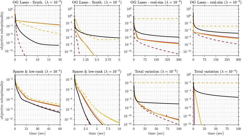
Figure 1: Empirical comparison of 5 algorithms for Problem (1) with smooth $f$. Dashed lines represent the line-search variants of TOS and PDHG. The performance of AdapTos is between TOS-LS and PDHG-LS. TOS and PDHG require the knowledge of the smoothness constant, and TOS-LS uses the Lipschitz constant for one of the nonsmooth terms.

In this subsection, we compare AdapTos with TOS, PDHG and their line-search variants TOS-LS and PDHG-LS. Our experiments are based on the benchmarks described in (Pedregosa & Gidel, 2018) and their source code available in COPT Library (Pedregosa et al., 2020) under the new BSD License. We implement AdapTos and investigate its performance on three different problems:

$\triangleright$ Logistic regression with overlapping group lasso penalty:

$$\min_{x\in\mathbb{R}^{n}}\quad\frac{1}{N}\sum_{i=1}^{N}\log(1+\exp(-b_{i}\langle a_{i},x\rangle))+\lambda\sum_{G\in\mathcal{G}}\sqrt{|G|}\|x_{G}\|+\lambda\sum_{H\in\mathcal{H}}\sqrt{|H|}\|x_{H}\|,$$ (27)

where $\{({a}_{1},{b}_{1}),\ldots,({a}_{N},{b}_{N})\}$ is a given set of training examples, $\mathcal{G}$ and $\mathcal{H}$ are the sets of distinct groups and $|\cdot|$ denotes the cardinality. The model we use (from COPT) considers groups of size $10$ with $2$ overlapping coefficients. In this experiment, we use the benchmarks on synthetic data (dimensions $n=1002$, $N=100$) and real-sim dataset (Chang & Lin, 2011) ($n=20958$, $N=72309$).

$\triangleright$ Image recovery with total variation penalty:

$$\min_{X\in\mathbb{R}^{m\times n}}\quad\|Y-\mathcal{A}(X)\|_{F}^{2}+\lambda\sum_{i=1}^{m}\sum_{j=1}^{n-1}|X_{i,j+1}-X_{i,j}|+\lambda\sum_{j=1}^{n}\sum_{i=1}^{m-1}|X_{i+1,j}-X_{i,j}|,$$ (28)

where $Y$ is a given blurred image and $\mathcal{A}:\mathbb{R}^{m\times n}\to\mathbb{R}^{m\times n}$ is a linear operator (blur kernel). The benchmark in COPT solves this problem for an image of size $153\times 115$ with a provided blur kernel.

$\triangleright$ Sparse and low-rank matrix recovery via $\ell_{1}$ and nuclear-norm regularizations:

$$\min_{X\in\mathbb{R}^{n\times n}}\quad\frac{1}{N}\sum_{i=1}^{N}\texttt{huber}(b_{i}-\langle A_{i},X\rangle)+\lambda\|X\|_{*}+\lambda\|X\|_{1}.$$ (29)

We use huber loss. $\{(A_{1},b_{1}),\ldots,(A_{N},b_{N})\}$ is a given set of measurements and $\|X\|_{1}$ is the vector $\ell_{1}$-norm of $X$. The benchmark in COPT considers a symmetric ground truth matrix $X^{\natural}\in\mathbb{R}^{20\times 20}$ and noisy synthetic measurements ($N=100$) where $A_{i}$ has Gaussian iid entries. $b_{i}=\langle A_{i},X^{\natural}\rangle+\omega_{i}$ where $\omega_{i}$ is generated from a zero-mean unit variance Gaussian distribution.

At each problem, we consider two different values for the regularization parameter $\lambda$. We use all methods with their default parameters in the benchmark. For AdapTos, we discard $\beta$ and tune $\alpha$ by trying the powers of $10$. See the supplementary material for the behavior of the algorithm with different values of $\alpha$. Figure 1 shows the results of this experiment. In most cases, the performance of AdapTos is between TOS-LS and PDHG-LS. Remark that TOS-LS is using the extra knowledge of the Lipschitz constant of $h$.

6.2 Experiments on Convex Optimization with Nonsmooth $f$

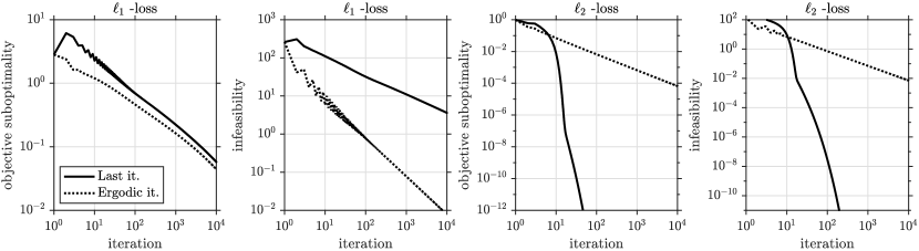
Figure 2: Performance of AdapTos on image impainting and denoising problems with $\ell_{1}$ and $\ell_{2}$-loss functions. The empirical rates for $\ell_{1}$-loss match the guaranteed $\smash{\mathcal{O}(1/\sqrt{t})}$ rate in objective suboptimality and $\smash{\mathcal{O}(1/t)}$ in infeasibility. We observe a locally linear convergence rate for the $\ell_{2}$-loss.

We examine the empirical performance of AdapTos for nonsmooth problems on an image impainting and denoising task from (Zeng & So, 2018; Yurtsever et al., 2018). We are given an occluded image (i.e., missing some pixels) of size $517\times 493$, contaminated with salt and pepper noise of $10\%$ density. We use the following template where data fitting is measured in terms of vector $\ell_{p}$-norm:

$$\min_{\bm{X}\in\mathbb{R}^{m\times n}}\quad\|\mathcal{A}(X)-Y\|_{p}\quad\text{subject to}\quad\|X\|_{\ast}\leq\lambda,~{}~{}~{}0\leq X\leq 1,$$ (30)

where $Y$ is the observed noisy image with missing pixels. This is essentially a matrix completion problem, $\mathcal{A}:\mathbb{R}^{m\times n}\to\mathbb{R}^{m\times n}$ is a linear map that samples the observed pixels in $Y$. In particular, we consider (30) with $p=1$ and $p=2$. The $\ell_{2}$-loss is common in practice for matrix completion (often in the least-squares form) but it is not robust against the outliers induced by the salt and pepper noise. $\ell_{1}$-loss is known to be more reliable for this task.

The subgradients in both cases have a fixed norm at all points (note that the subgradients are binary valued for $\ell_{1}$-loss and unit-norm for $\ell_{2}$-loss), hence the analytical and the adaptive step-sizes are same up to a constant factor.

Figure 2 shows the results. The empirical rates for $p=1$ roughly match our guarantees in Theorem 1. We observe a locally linear convergence rate when $\ell_{2}$-loss is used. Interestingly, the ergodic sequence converges faster than the last iterate for $p=1$ but significantly slower for $p=2$. The runtime of the two settings are approximately the same, with 67 msec per iteration on average. Despite the slower rates, we found $\ell_{1}$-loss more practical on this problem. A low-accuracy solution obtained by $1000$ iterations on $\ell_{1}$-loss yields a high quality recovery with PSNR 26.21 dB, whereas the PSNR saturates at 21.15 dB for the $\ell_{2}$-formulation. See the supplements for the recovered images and more details.

6.3 An Experiment on Neural Networks

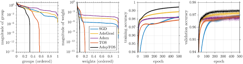
Figure 3: Comparison of methods on training neural networks with group lasso regularization. The outgoing connections of each neuron form a group. The first plot shows the magnitude of weights after 500 epochs. The second plot shows the absolute sum of outgoing weights from each neuron. x-axes are normalized by the total number of weights and neurons in these plots. More than 68% of the neurons are inactive on the network trained by AdapTos. The third and fourth plots show the training and validation losses. This experiment is performed with 20 random seeds. The solid lines show the average performance and the shaded area represents $\pm$ standard deviation from the mean.

In this section, we train a regularized deep neural network to test our methods on nonconvex optimization. We consider a regularized neural network problem formulation in (Scardapane et al., 2017). This problem involves a fully connected neural network with the standard cross-entropy loss function, a ReLu activation for the hidden layers, and the softmax activation for the output layer. Two regularizers are added to this loss function: The first one is the standard $\ell_{1}$ regularizer, and the second is the group sparse regularizer where the outgoing connections of each neuron is considered as a group. The goal is to force all outgoing connections from the same neurons to be simultaneously zero, so that we can safely remove the neurons from the network. This is shown as an effective way to obtain compact networks (Scardapane et al., 2017), which is crucial for the deployment of the learned parameters on resource-constrained devices such as smartphones (Blalock et al., 2020).

We reuse the open source implementation (built with Lasagne framework based on Theano) published in (Scardapane et al., 2017) under BSD-2 License. We follow their experimental setup and instructions with MNIST database (LeCun, 1998) containing 70k grayscale images ($28\times 28$) of handwritten digits (split 75/25 into train and test partitions). We train a fully connected neural network with $784$ input features, three hidden layers ($400/300/100$) and 10-dimensional output layer. Interested readers can find more details on the implementation in the supplementary material or in (Scardapane et al., 2017).

Scardapane et al. (2017) use SGD and Adam with the subgradient of the overall objective. In contrast, our methods can leverage the prox-operators for the regularizers. Figure 3 compares the performance in terms of two measures: the sparsity of the parameters and the accuracy. On the left side, we see the spectrum of weight and neuron magnitudes. The advantage of using prox-operators is outstanding: More than 93% of the weights are zero and 68% of neurons are inactive when trained with AdapTos. In contrast, subgradient based methods can achieve only approximately sparse solutions.

The third and the fourth subplots present the training and test accuracies. Remarkably, AdapTos performs better than the state-of-the-art (both in train and test). Unfortunately, we could not achieve the same performance gain in preliminary experiments with more complex models like ResNet (He et al., 2016), where SGD with momentum shines. Interested readers can find the code for these preliminary experiments in the supplements. We leave the technical analysis and a comprehensive examination of AdapTos for nonconvex problems to a future work.

7 Conclusions

We studied an extension of TOS that permits subgradients and stochastic gradients instead of the gradient step and established convergence guarantees for this extension. Moreover, we proposed an adaptive step-size rule (AdapTos) for the minimization of a convex function over the intersection of two convex sets. AdapTos guarantees a nearly optimal $\tilde{\mathcal{O}}(1/\sqrt{t})$ rate on the baseline setting, and it enjoys the faster $\tilde{\mathcal{O}}(1/t)$ rate when the problem is smooth and the solution is in the interior of feasible set. We present numerical experiments on various benchmark problems. The empirical performance of the method is promising.

We conclude with a short list of open questions and follow-up directions: (i) In parallel to the subgradient method, we believe TOS can achieve $\mathcal{O}(1/t)$ rate guarantees in the nonsmooth setting if $f$ is strongly convex. The analysis remains open. (ii) The faster rate for AdapTos on smooth $f$ requires an extra assumption on the location of the solution. We believe this assumption can be removed, and leave this as an open problem. (iii) We analyzed AdapTos only for a specific subclass of Problem (1) in which $g$ and $h$ are indicator functions. Extending this result for the whole class is a valuable question for future study.

Appendix A Preliminaries

We will use the following standard results in our analysis.

Lemma S.2.

Let $f:\mathbb{R}^{n}\to\mathbb{R}\cup\{+\infty\}$ be a proper closed and convex function. Then, for any $x,u\in\mathbb{R}^{n}$, the followings are equivalent:

1. $u=\mathrm{prox}_{f}(x)$.

2. $x-u\in\partial f(u)$.

3. $\langle x-u,y-u\rangle\leq f(y)-f(u)$  for any  $y\in\mathbb{R}^{n}$.
   

Corollary 2 (Firm non-expansivity of the prox-operator).

Let $f:\mathbb{R}^{n}\to\mathbb{R}\cup\{+\infty\}$ be a proper closed and convex function. Then, for any $x,u\in\mathbb{R}^{n}$, the followings hold:

(non-expansivity) $$\|\mathrm{prox}_{f}(x)-\mathrm{prox}_{f}(y)\|\leq\|x-y\|.$$

(firm non-expansivity) $$\|\mathrm{prox}_{f}(x)-\mathrm{prox}_{f}(y)\|^{2}\leq\langle x-y,\mathrm{prox}_{f}(x)-\mathrm{prox}_{f}(y)\rangle.$$

Appendix B Fixed Point Characterization

This appendix presents the proof for Lemma 1. This is a straightforward extension of Lemma 2.2 in (Davis & Yin, 2017) to permit subgradients. We will use this lemma in the next section to prove the boundedness of $y_{t}$ in Algorithm 1.

B.1 Proof of Lemma 1

Define $z=\mathrm{prox}_{\gamma g}(y)$ and $x=\mathrm{prox}_{\gamma h}(2z-y-\gamma u)$. Then, $\texttt{TOS}_{\gamma}(y,u):=y-z+x$.

Suppose there exists $u\in\partial f(z)$ such that $\texttt{TOS}(y,u)=y$. Then, we must have $z=x$. Moreover, by Lemma S.2, we have

$$z=\mathrm{prox}_{\gamma g}(y) \iff y-z\in\gamma\partial g(z),$$ (S.1)

$$\text{and}\quad z=x=\mathrm{prox}_{\gamma h}(2z-y-\gamma u) \iff z-y-\gamma u\in\gamma\partial h(x).$$ (S.2)

By summing up (S.1) and (S.2), we observe

$$0\in\gamma(u+\partial g(z)+\partial h(x))\implies 0\in\partial f(z)+\partial g(z)+\partial h(z)=\partial\phi(z),$$ (S.3)

which proves that $z$ is an optimal solution of Problem (1) since $\phi$ is convex.

To prove the reverse direction, suppose $z$ is an optimal solution, i.e., there exists $u\in\partial f(z),v\in\partial g(z),w\in\partial h(z)$ such that $u+v+w=0$. By Lemma S.2, we have

$$z=\mathrm{prox}_{\gamma g}(y) \iff y-z\in\gamma\partial g(z),$$ (S.4)

$$\text{and}\quad x=\mathrm{prox}_{\gamma h}(2z-y-\gamma u) \iff 2z-x-y-\gamma u\in\gamma\partial h(x).$$ (S.5)

Now, let $y=z+\gamma v$. Then,

$$2z-x-y-\gamma u=z-x-\gamma(u+v)=z-x+\gamma w.$$ (S.6)

Therefore, we have $z-x+\gamma w\in\partial h(x)$. Again, due to Lemma S.2, this means $x=\mathrm{prox}_{\gamma h}(z+\gamma w)$. We also know $w\in\partial h(z)\iff z+\gamma w-z\in\partial\gamma h(z)\iff z=\mathrm{prox}_{\gamma h}(z+\gamma w)$. However, since $h$ is convex, its prox-operator is unique, hence, $x=z$ and $\texttt{TOS}_{\gamma}(y,u)=y$.

Appendix C Boundedness Guarantees

Theorem S.6.

Consider Problem (1) and employ TOS (Algorithm 1) with subgradient steps ${u_{t}\in\partial f(z_{t})}$ and a fixed step-size $\gamma=\gamma_{0}/\sqrt{T+1}$ for some $\gamma_{0}>0$. Assume that $\|u_{t}\|\leq G_{f}$ for all $t$. Then,

$$\|y_{T+1}-y_{\star}\|\leq\|y_{0}-y_{\star}\|+2\gamma_{0}G_{f}$$ (S.7)

where $y_{\star}$ is a fixed point of TOS.

Proof.

By Lemma 1, there exists $u_{\star}\in\partial f(x_{\star})$ such that

$$x_{\star}=\mathrm{prox}_{\gamma g}(y_{\star})=\mathrm{prox}_{\gamma h}(2x_{\star}-y_{\star}-\gamma u_{\star})=z_{\star}.$$ (S.8)

We decompose $\|y_{t+1}-y_{\star}\|^{2}$ as

$$\|y_{t+1}-y_{\star}\|^{2} =\|y_{t}-z_{t}+x_{t}-y_{\star}+x_{\star}-x_{\star}\|^{2}$$

$$=\|y_{t}-z_{t}-y_{\star}+x_{\star}\|^{2}+\|x_{t}-x_{\star}\|^{2}+2\langle x_{t}-x_{\star},y_{t}-z_{t}-y_{\star}+x_{\star}\rangle.$$ (S.9)

Since $z_{t}=\mathrm{prox}_{\gamma g}(y_{t})$ and $x_{\star}=\mathrm{prox}_{\gamma g}(y_{\star})$, by the firm non-expansivity of the prox-operator, we have

$$\|y_{t}-z_{t}-y_{\star}+x_{\star}\|^{2} =\langle y_{t}-z_{t}-y_{\star}+x_{\star},y_{t}-y_{\star}\rangle-\langle y_{t}-z_{t}-y_{\star}+x_{\star},z_{t}-x_{\star}\rangle$$

$$\leq\langle y_{t}-z_{t}-y_{\star}+x_{\star},y_{t}-y_{\star}\rangle.$$ (S.10)

Similarly, since $x_{t}=\mathrm{prox}_{\gamma h}(2z_{t}-y_{t}-\gamma u_{t})$ and $x_{\star}=\mathrm{prox}_{\gamma h}(2x_{\star}-y_{\star}-\gamma u_{\star})$, by the firm non-expansivity of the prox-operator, we have

$$\|x_{t}-x_{\star}\|^{2}\leq\langle x_{t}-x_{\star},(2z_{t}-y_{t}-\gamma u_{t})-(2x_{\star}-y_{\star}-\gamma u_{\star})\rangle.$$ (S.11)

By combining (S.9), (S.10) and (S.11), we get

$$\|y_{t+1}-y_{\star}\|^{2} \leq\langle y_{t}-z_{t}+x_{t}-y_{\star},y_{t}-y_{\star}\rangle-\gamma\langle x_{t}-x_{\star},u_{t}-u_{\star}\rangle$$

$$=\langle y_{t+1}-y_{\star},y_{t}-y_{\star}\rangle-\gamma\langle x_{t}-x_{\star},u_{t}-u_{\star}\rangle$$

$$=\frac{1}{2}\|y_{t+1}-y_{\star}\|^{2}+\frac{1}{2}\|y_{t}-y_{\star}\|^{2}-\frac{1}{2}\|y_{t+1}-y_{t}\|^{2}-\gamma\langle x_{t}-x_{\star},u_{t}-u_{\star}\rangle.$$ (S.12)

Since $u_{t}\in\partial f(z_{t})$ and $u_{\star}\in\partial f(x_{\star})$, we have

$$-\langle x_{t}-x_{\star},u_{t}-u_{\star}\rangle =-\langle z_{t}-x_{\star},u_{t}-u_{\star}\rangle-\langle x_{t}-z_{t},u_{t}-u_{\star}\rangle$$

$$\leq-\langle x_{t}-z_{t},u_{t}-u_{\star}\rangle$$

$$\leq\frac{1}{2\gamma}\|x_{t}-z_{t}\|^{2}+\frac{\gamma}{2}\|u_{t}-u_{\star}\|^{2},$$ (S.13)

where we used Young’s inequality in the last line. We use this inequality in (S.12) to obtain

$$\|y_{t+1}-y_{\star}\|^{2}\leq\|y_{t}-y_{\star}\|^{2}+\gamma^{2}\|u_{t}-u_{\star}\|^{2}.$$ (S.14)

If we sum this inequality from $t=0$ to $T$, we get

$$\|y_{T+1}-y_{\star}\|^{2}\leq\|y_{0}-y_{\star}\|^{2}+\gamma^{2}\sum_{\tau=0}^{T}\|u_{\tau}-u_{\star}\|^{2}.$$ (S.15)

Finally, due to the bounded subgradients assumption, we have $\|u_{\tau}-u_{\star}\|\leq 2G_{f}$, hence

$$\|y_{T+1}-y_{\star}\|^{2} \leq\|y_{0}-y_{\star}\|^{2}+4G_{f}^{2}\gamma^{2}(T+1)=\|y_{0}-y_{\star}\|^{2}+4G_{f}^{2}\gamma_{0}^{2}.$$ (S.16)

We complete the proof by taking the square-root of both sides,

$$\|y_{T+1}-y_{\star}\|\leq\sqrt{\|y_{0}-y_{\star}\|^{2}+4G_{f}^{2}\gamma_{0}^{2}}\leq\|y_{0}-y_{\star}\|+2G_{f}\gamma_{0}.$$ (S.17)

∎

Theorem S.7.

Consider Problem (14) and employ TOS (Algorithm 1) with a fixed step-size $\gamma=\gamma_{0}/\sqrt{T+1}$ for some $\gamma_{0}>0$. Suppose we are receiving the update directions $u_{t}$ from an unbiased stochastic first-order oracle with bounded variance such that

$$\hat{u}_{t}:=\mathbb{E}[u_{t}|z_{t}]\in\partial f(z_{t})\quad\text{and}\quad\mathbb{E}[\|u_{t}-\hat{u}_{t}\|^{2}]\leq\sigma^{2}~{}~{}\text{for some $\sigma<+\infty$.}$$ (S.18)

Assume that $\|\hat{u}_{t}\|\leq G_{f}$ for all $t$. Then,

$$\mathbb{E}[\|y_{T+1}-y_{\star}\|]\leq\|y_{0}-y_{\star}\|+\gamma_{0}(2G_{f}+\sigma)$$ (S.19)

where $y_{\star}$ is a fixed point of TOS.

Proof.

We follow the same steps as in the proof of Theorem S.6 until (S.12):

$$\|y_{t+1}-y_{\star}\|^{2} \leq\|y_{t}-y_{\star}\|^{2}-\|y_{t+1}-y_{t}\|^{2}-2\gamma\langle x_{t}-x_{\star},u_{t}-u_{\star}\rangle.$$ (S.20)

Then, we need to take noise into account:

$$-\langle x_{t}-x_{\star},u_{t}-u_{\star}\rangle =-\langle x_{t}-z_{t},u_{t}-u_{\star}\rangle-\langle z_{t}-x_{\star},u_{t}-\hat{u}_{t}\rangle-\langle z_{t}-x_{\star},\hat{u}_{t}-u_{\star}\rangle$$

$$\leq-\langle x_{t}-z_{t},u_{t}-u_{\star}\rangle-\langle z_{t}-x_{\star},u_{t}-\hat{u}_{t}\rangle.$$ (S.21)

We take the expectation of both sides and get

$$-\mathbb{E}[\langle x_{t}-x_{\star},u_{t}-u_{\star}\rangle] \leq-\mathbb{E}[\langle x_{t}-z_{t},u_{t}-u_{\star}\rangle]$$

$$\leq\frac{1}{2\gamma}\mathbb{E}[\|x_{t}-z_{t}\|^{2}]+\frac{\gamma}{2}\mathbb{E}[\|u_{\star}-u_{t}\|^{2}]$$

$$=\frac{1}{2\gamma}\mathbb{E}[\|x_{t}-z_{t}\|^{2}]+\frac{\gamma}{2}\mathbb{E}[\|u_{\star}-\hat{u}_{t}\|^{2}]+\frac{\gamma}{2}\mathbb{E}[\|\hat{u}_{t}-u_{t}\|^{2}]$$

$$\leq\frac{1}{2\gamma}\mathbb{E}[\|x_{t}-z_{t}\|^{2}]+2\gamma G_{f}^{2}+\frac{\gamma}{2}\sigma^{2},$$ (S.22)

where the last line holds due to the bounded subgradients and variance assumptions.

Now, we take the expectation of (S.20) and substitute (S.22) into it:

$$\mathbb{E}[\|y_{t+1}-y_{\star}\|^{2}]\leq\mathbb{E}[\|y_{t}-y_{\star}\|^{2}]+\gamma^{2}(4G_{f}^{2}+\sigma^{2}).$$ (S.23)

Finally, we sum this inequality over $t=0,1,\ldots,T$:

$$\mathbb{E}[\|y_{T+1}-y_{\star}\|^{2}]\leq\|y_{0}-y_{\star}\|^{2}+\gamma_{0}^{2}(4G_{f}^{2}+\sigma^{2}).$$ (S.24)

By Jensen’s inequality, we have $\mathbb{E}[\|y_{T+1}-y_{\star}\|]^{2}\leq\mathbb{E}[\|y_{T+1}-y_{\star}\|^{2}]$. We finalize the proof by taking the square-root of both sides. ∎

Next, we assume that $f$ is $L_{f}$-smooth instead of Lipschitz continuity.

Theorem S.8.

Consider Problem (14) and suppose $f$ is $L_{f}$-smooth on $\mathrm{dom}(g)$. Employ TOS (Algorithm 1) with a fixed step-size $\gamma_{t}=\gamma=\gamma_{0}/\sqrt{T+1}$ for some $\gamma_{0}\in[0,\frac{2}{L_{f}}]$. Suppose we are receiving the update directions $u_{t}$ from an unbiased stochastic first-order oracle with bounded variance such that

$$\mathbb{E}[u_{t}|z_{t}]=\nabla f(z_{t})\quad\text{and}\quad\mathbb{E}[\|u_{t}-\nabla f(z_{t})\|^{2}]\leq\sigma^{2}~{}~{}\text{for some $\sigma<+\infty$.}$$ (S.25)

Then,

$$\mathbb{E}[\|y_{T+1}-y_{\star}\|]\leq\|y_{0}-y_{\star}\|+2\sigma\sqrt{\frac{\gamma_{0}}{L_{f}}},$$ (S.26)

where $y_{\star}$ is a fixed point of TOS.

Proof.

The proof is similar to the proof of Theorem S.7. We start from (S.20) and take the expectation:

$$\mathbb{E}[\|y_{t+1}-y_{\star}\|^{2}] \leq\mathbb{E}[\|y_{t}-y_{\star}\|^{2}]-\mathbb{E}[\|y_{t+1}-y_{t}\|^{2}]-2\gamma\mathbb{E}[\langle x_{t}-x_{\star},u_{t}-u_{\star}\rangle].$$ (S.27)

We decompose the last term as follows:

$$\mathbb{E}[\langle x_{t}-x_{\star},u_{\star}-u_{t}\rangle] =\mathbb{E}[\langle x_{t}-z_{t},u_{\star}-u_{t}\rangle]+\mathbb{E}[\langle z_{t}-x_{\star},u_{\star}-\nabla f(z_{t})\rangle]+\mathbb{E}[\langle z_{t}-x_{\star},\nabla f(z_{t})-u_{t}\rangle]$$

$$\leq\mathbb{E}[\langle x_{t}-z_{t},u_{\star}-u_{t}\rangle]-\frac{1}{L_{f}}\mathbb{E}[\|u_{\star}-\nabla f(z_{t})\|^{2}].$$ (S.28)

where the inequality holds since $f$ is $L_{f}$-smooth and convex. Moreover, we can bound the inner product term by using Young’s inequality as follows:

$$\mathbb{E}[\langle x_{t}-z_{t},u_{\star}-u_{t}\rangle] =\mathbb{E}\big{[}\langle x_{t}-z_{t},u_{\star}-\nabla f(z_{t})\rangle+\langle x_{t}-z_{t},\nabla f(z_{t})-u_{t}\rangle\big{]}$$

$$\leq\mathbb{E}\Big{[}\frac{c_{1}+c_{2}}{2}\|x_{t}-z_{t}\|^{2}+\frac{1}{2c_{1}}\|u_{\star}-\nabla f(z_{t})\|^{2}+\frac{1}{2c_{2}}\|\nabla f(z_{t})-u_{t}\|^{2}\Big{]}$$ (S.29)

for any $c_{1},c_{2}>0$. We choose $c_{1}=L_{f}/2$, so that the corresponding terms in (S.28) and (S.29) cancel out. Combining (S.27), (S.28) and (S.29), we get

$$\mathbb{E}[\|y_{t+1}-y_{\star}\|^{2}] \leq\mathbb{E}[\|y_{t}-y_{\star}\|^{2}]-\mathbb{E}[\|y_{t+1}-y_{t}\|^{2}]+\gamma(\tfrac{L_{f}}{2}+c_{2})\mathbb{E}[\|x_{t}-z_{t}\|^{2}]+\gamma\frac{\sigma^{2}}{c_{2}}$$

$$\leq\mathbb{E}[\|y_{t}-y_{\star}\|^{2}]+\Big{(}\gamma\frac{L_{f}+2c_{2}}{2}-1\Big{)}\mathbb{E}[\|x_{t}-z_{t}\|^{2}]+\gamma\frac{\sigma^{2}}{c_{2}}.$$ (S.30)

Then, we choose $c_{2}=\tfrac{L_{f}}{2}(\sqrt{T+1}-1)$. With the condition $\gamma_{0}\leq\tfrac{2}{L_{f}}$, this guarantees

$$\gamma\frac{L_{f}+2c_{2}}{2}-1=\frac{\gamma_{0}}{\sqrt{T+1}}\frac{L_{f}\sqrt{T+1}}{2}-1\leq\gamma_{0}\frac{L_{f}}{2}-1\leq 0.$$ (S.31)

Returning to (S.30), we now have

$$\mathbb{E}[\|y_{t+1}-y_{\star}\|^{2}] \leq\mathbb{E}[\|y_{t}-y_{\star}\|^{2}]+\frac{\gamma_{0}}{\sqrt{T+1}}\frac{2\sigma^{2}}{L_{f}(\sqrt{T+1}-1)}\leq\mathbb{E}[\|y_{t}-y_{\star}\|^{2}]+\frac{4\gamma_{0}\sigma^{2}}{L_{f}(T+1)}.$$ (S.32)

Finally, we sum this inequality over $t=0$ to $T$,

$$\mathbb{E}[\|y_{T+1}-y_{\star}\|^{2}]\leq\|y_{0}-y_{\star}\|^{2}+\frac{4\gamma_{0}\sigma^{2}}{L_{f}}.$$ (S.33)

Remark that $\mathbb{E}[\|y_{T+1}-y_{\star}\|]^{2}\leq\mathbb{E}[\|y_{T+1}-y_{\star}\|^{2}]$. We finish the proof by taking the square-root of both sides. ∎

Appendix D Convergence Guarantees

This section presents the technical analysis of our main results.

D.1 Proof of Theorem 1

We divide this proof into two parts.

Part 1. In the first part, we show that the sequence generated by TOS satisfies

$$\langle u_{t},x_{t}-x_{\star}\rangle+g(z_{t})-g(x_{\star})+h(x_{t})-h(x_{\star})\leq\frac{1}{2\gamma}\|y_{t}-x_{\star}\|^{2}-\frac{1}{2\gamma}\|y_{t+1}-x_{\star}\|^{2}-\frac{1}{2\gamma}\|y_{t+1}-y_{t}\|^{2}.$$ (S.34)

Since $x_{t}=\mathrm{prox}_{\gamma h}(2z_{t}-y_{t}-\gamma u_{t})$, by Lemma S.2, we have

$$\langle 2z_{t}-y_{t}-\gamma u_{t}-x_{t},x_{\star}-x_{t}\rangle\leq\gamma h(x_{\star})-\gamma h(x_{t}).$$ (S.35)

We rearrange this inequality as follows:

$$\langle u_{t},x_{t}-x_{\star}\rangle+h(x_{t})- h(x_{\star})\leq\frac{1}{\gamma}\langle 2z_{t}-y_{t}-x_{t},x_{t}-x_{\star}\rangle$$

$$=\frac{1}{\gamma}\langle z_{t}-y_{t},z_{t}-x_{\star}\rangle+\frac{1}{\gamma}\langle z_{t}-y_{t},x_{t}-z_{t}\rangle+\frac{1}{\gamma}\langle z_{t}-x_{t},x_{t}-x_{\star}\rangle$$

$$=\frac{1}{\gamma}\langle z_{t}-y_{t},z_{t}-x_{\star}\rangle+\frac{1}{\gamma}\langle y_{t}+x_{t}-z_{t}-x_{\star},z_{t}-x_{t}\rangle$$

$$=\frac{1}{\gamma}\langle z_{t}-y_{t},z_{t}-x_{\star}\rangle+\frac{1}{\gamma}\langle y_{t+1}-x_{\star},y_{t}-y_{t+1}\rangle.$$ (S.36)

Then, we use Lemma S.2 once again (for $\gamma g$) and get

$$\langle u_{t},x_{t}-x_{\star}\rangle+g(z_{t})-g(x_{\star})+h(x_{t})-h(x_{\star}) \leq\frac{1}{\gamma}\langle y_{t+1}-x_{\star},y_{t}-y_{t+1}\rangle$$

$$\leq\frac{1}{2\gamma}\|y_{t}-x_{\star}\|^{2}-\frac{1}{2\gamma}\|y_{t+1}-x_{\star}\|^{2}-\frac{1}{2\gamma}\|y_{t+1}-y_{t}\|^{2}.$$ (S.37)

This completes the first part of the proof.

Part 2. In the second part, we characterize the convergence rate of $f(\bar{z}_{t})+g(\bar{z}_{t})+h(\bar{x}_{t})-\phi_{\star}$ to $0$ by using (S.34). Since $f$ is convex, we have

$$\langle u_{t},x_{t}-x_{\star}\rangle=\langle u_{t},z_{t}-x_{\star}\rangle-\langle u_{t},z_{t}-x_{t}\rangle \geq f(z_{t})-f(x_{\star})-\frac{1}{2\gamma}\|x_{t}-z_{t}\|^{2}-\frac{\gamma}{2}\|u_{t}\|^{2}.$$ (S.38)

By combining (S.34) and (S.38), we obtain

$$f(z_{t})+g(z_{t})+h(x_{t})-\phi_{\star}\leq\frac{1}{2\gamma}\|y_{t}-x_{\star}\|^{2}-\frac{1}{2\gamma}\|y_{t+1}-x_{\star}\|^{2}+\frac{\gamma}{2}\|u_{t}\|^{2}.$$ (S.39)

We sum this inequality over $t=0$ to $T$:

$$\sum_{\tau=0}^{T}\Big{(}f(z_{\tau})+g(z_{\tau})+h(x_{\tau})-\phi_{\star}\Big{)} \leq\frac{1}{2\gamma}\|y_{0}-x_{\star}\|^{2}+\frac{\gamma}{2}\sum_{\tau=0}^{T}\|u_{\tau}\|^{2}\leq\frac{1}{2\gamma}\|y_{0}-x_{\star}\|^{2}+\frac{\gamma_{0}}{2}G_{f}^{2}\sqrt{T+1},$$ (S.40)

where the second inequality holds due to the bounded subgradients assumption. Finally, we divide both sides by $(T+1)$ and use Jensen’s inequality:

$$f(\bar{z}_{t})+g(\bar{z}_{t})+h(\bar{x}_{t})-\phi_{\star}\leq\frac{1}{2\sqrt{T+1}}\left(\frac{1}{\gamma_{0}}\|y_{0}-x_{\star}\|^{2}+\gamma_{0}G_{f}^{2}\right).$$ (S.41)

D.2 Proof of Theorem 2

The proof is similar to the proof of Theorem 1. We will only discuss the different steps. Part 1 of the proof is the same, i.e., (S.34) is still valid.

We need to consider the randomness of the gradient estimator in the second part. To this end, we modify (S.38) as:

$$\mathbb{E}[\langle u_{t},x_{t}-x_{\star}\rangle] =\mathbb{E}[\langle\hat{u}_{t},z_{t}-x_{\star}\rangle]+\mathbb{E}[\langle u_{t}-\hat{u}_{t},z_{t}-x_{\star}\rangle]-\mathbb{E}[\langle u_{t},z_{t}-x_{t}\rangle]$$

$$\geq\mathbb{E}[f(z_{t})-f(x_{\star})]-\mathbb{E}[\langle u_{t},z_{t}-x_{t}\rangle]$$

$$\geq\mathbb{E}[f(z_{t})-f(x_{\star})]-\frac{1}{2\gamma}\mathbb{E}[\|z_{t}-x_{t}\|^{2}]-\frac{\gamma}{2}\mathbb{E}[\|u_{t}\|^{2}]$$

$$\geq\mathbb{E}[f(z_{t})-f(x_{\star})]-\frac{1}{2\gamma}\mathbb{E}[\|z_{t}-x_{t}\|^{2}]-\frac{\gamma}{2}(G_{f}^{2}+\sigma^{2}),$$ (S.42)

where the last line holds since

$$\mathbb{E}[\|u_{t}\|^{2}] =\mathbb{E}[\|u_{t}-\hat{u}_{t}+\hat{u}_{t}\|^{2}]$$ (S.43)

$$=\mathbb{E}[\|u_{t}-\hat{u}_{t}\|^{2}]+\mathbb{E}[\|\hat{u}_{t}\|^{2}]+2\mathbb{E}[\langle u_{t}-\hat{u}_{t},\hat{u}_{t}\rangle]\leq\sigma^{2}+G_{f}^{2}.$$ (S.44)

Now, we take the expectation of (S.34) and substitute (S.42) into it:

$$\mathbb{E}[f(z_{t})+g(z_{t})+h(x_{t})]-\phi_{\star}\leq\frac{1}{2\gamma}\mathbb{E}[\|y_{t}-x_{\star}\|^{2}]-\frac{1}{2\gamma}\mathbb{E}[\|y_{t+1}-x_{\star}\|^{2}]+\frac{\gamma}{2}(\sigma^{2}+G_{f}^{2}).$$ (S.45)

We sum this inequality from $t=0$ to $T$ and divide both sides by $T+1$. Then, we use Jensen’s inequality and get

$$\mathbb{E}[f(\bar{z}_{T})+g(\bar{z}_{T})+h(\bar{x}_{T})]-\phi_{\star}\leq\frac{1}{2\sqrt{T+1}}\left(\frac{1}{\gamma_{0}}\|y_{0}-x_{\star}\|^{2}+\gamma_{0}(\sigma^{2}+G_{f}^{2})\right).$$ (S.46)

D.3 TOS for the Smooth and Stochastic Setting (Remark 3)

Theorem S.9.

Consider Problem (14) and suppose $f$ is $L_{f}$-smooth on $\mathrm{dom}(g)$. Employ TOS (Algorithm 1) with a fixed step-size $\gamma=\gamma_{0}/\sqrt{T+1}$ for some $\gamma_{0}\in[0,\frac{1}{2L_{f}}]$. Suppose we are receiving the update directions $u_{t}$ from an unbiased stochastic first-order oracle with bounded variance such that

$$\mathbb{E}[u_{t}|z_{t}]=\nabla f(z_{t})\quad\text{and}\quad\mathbb{E}[\|u_{t}-\nabla f(z_{t})\|^{2}]\leq\sigma^{2}~{}~{}\text{for some $\sigma<+\infty$.}$$ (S.47)

Then, the following guarantees hold:

$$\mathbb{E}[f(\bar{x}_{T})+g(\bar{z}_{T})+h(\bar{x}_{T})]-\phi_{\star}\leq\frac{1}{\sqrt{T+1}}\left(\frac{D^{2}}{2\gamma_{0}}+\gamma_{0}\sigma^{2}\right),~{}~{}~{}\text{where}~{}~{}~{}D=\|y_{0}-x_{\star}\|.$$ (S.48)

Proof.

The proof is similar to Theorem 1. (S.34) still holds. We modify (S.38) as follows (similar to (S.42)):

$$\mathbb{E}[\langle u_{t},x_{t}-x_{\star}\rangle] \geq\mathbb{E}[f(z_{t})-f(x_{\star})]+\mathbb{E}[\langle\nabla f(z_{t})-u_{t},z_{t}-x_{t}\rangle]-\mathbb{E}[\langle\nabla f(z_{t}),z_{t}-x_{t}\rangle]$$

$$\geq\mathbb{E}[f(x_{t})-f(x_{\star})]-\frac{1}{4\gamma}\mathbb{E}[\|z_{t}-x_{t}\|^{2}]-\gamma\mathbb{E}[\|\nabla f(z_{t})-u_{t}\|^{2}]-\frac{L_{f}}{2}\|x_{t}-z_{t}\|^{2}$$

$$\geq\mathbb{E}[f(x_{t})-f(x_{\star})]-\frac{1+2\gamma L_{f}}{4\gamma}\mathbb{E}[\|y_{t+1}-y_{t}\|^{2}]-\gamma\sigma^{2}.$$ (S.49)

We take the expectation of (S.34) and replace (S.49) into it

$$\mathbb{E}[f(x_{t})+g(z_{t})+h(x_{t})]-\phi_{\star} \leq\frac{1}{2\gamma}\|y_{t}-x_{\star}\|^{2}-\frac{1}{2\gamma}\|y_{t+1}-x_{\star}\|^{2}+\frac{2\gamma L_{f}-1}{4\gamma}\mathbb{E}[\|y_{t+1}-y_{t}\|^{2}]+\gamma\sigma^{2}$$

$$\leq\frac{1}{2\gamma}\|y_{t}-x_{\star}\|^{2}-\frac{1}{2\gamma}\|y_{t+1}-x_{\star}\|^{2}+\gamma\sigma^{2},$$ (S.50)

where the second line holds since we choose $\gamma_{0}\in[0,\frac{1}{2L_{f}}]$.

We sum (S.50) from $t=0$ to $T$ and divide both sides by $T+1$. We complete the proof by using Jensen’s inequality. ∎

Appendix E Convergence Guarantees for AdapTos

In this section, we focus on Problem (18), an important subclass of Problem (1) where $g$ and $h$ are indicator functions. In this setting, TOS performs the following steps iteratively for $t=0,1,\ldots$:

$$z_{t} =\mathrm{proj}_{\mathcal{G}}(y_{t})$$ (S.51)

$$x_{t} =\mathrm{proj}_{\mathcal{H}}(2z_{t}-y_{t}-\gamma_{t}u_{t})$$ (S.52)

$$y_{t+1} =y_{t}-z_{t}+x_{t},$$ (S.53)

where $\gamma_{t}$ at line (S.52) is chosen according to the adaptive step-size rule (19), i.e.,

$$\gamma_{t}=\frac{\alpha}{\sqrt{\beta+\sum_{\tau=0}^{t-1}\|u_{\tau}\|^{2}}}\quad\text{for some $\alpha,\beta>0$.}$$ (S.54)

The following lemmas are useful in the analysis.

Lemma S.3 (Lemma A.2 in (Levy, 2017)).

Let $f:\mathbb{R}^{n}\to\mathbb{R}$ be a $L_{f}$-smooth function and let $x_{\star}\in\arg\min_{x\in\mathbb{R}^{n}}f(x)$. Then,

$$\|\nabla f(x)\|^{2}\leq 2L_{f}\big{(}f(x)-f(x_{\star})\big{)},\qquad\forall x\in\mathbb{R}^{n}.$$

Lemma S.4 (Lemma 9 in (Bach & Levy, 2019)).

For any non-negative numbers $a_{0},\ldots,a_{t}\in[0,a]$, and $\beta\geq 0$

$$\sum_{i=0}^{t}\frac{a_{i}}{\sqrt{\beta+\sum_{j=0}^{i-1}a_{j}}}\leq\frac{2a}{\sqrt{\beta}}+3\sqrt{a}+3\sqrt{\beta+\sum_{i=0}^{t-1}a_{i}}.$$

Lemma S.5 (Lemma 10 in (Bach & Levy, 2019)).

For any non-negative numbers $a_{0},\ldots,a_{t}\in[0,a]$, and $\beta\geq 0$

$$\sum_{i=0}^{t}\frac{a_{i}}{\beta+\sum_{j=0}^{i-1}a_{j}}\leq 2+\frac{4a}{\beta}+2\log\left(1+\sum_{i=0}^{t-1}\frac{a_{i}}{\beta}\right).$$

Corollary 3.

Suppose $\|u_{t}\|\leq G$ for all $t$. Then, the following relations hold for AdapTos:

$$(i).~{}~{} \sum_{\tau=0}^{t}\gamma_{\tau}\|u_{\tau}\|^{2}=\alpha\sum_{\tau=0}^{t}\frac{\|u_{\tau}\|^{2}}{\sqrt{\beta+\sum_{j=0}^{\tau-1}\|u_{j}\|^{2}}}\leq\alpha\left(\frac{2G^{2}}{\sqrt{\beta}}+3G+3\sqrt{\beta+G^{2}t}\right)$$

$$(ii).~{}~{} \sum_{\tau=0}^{t}\gamma_{\tau}^{2}\|u_{\tau}\|^{2}=\alpha^{2}\sum_{\tau=0}^{t}\frac{\|u_{\tau}\|^{2}}{\beta+\sum_{j=0}^{\tau-1}\|u_{j}\|^{2}}\leq\alpha^{2}\left(2+\frac{4G^{2}}{\beta}+2\log\Big{(}1+\frac{G^{2}}{\beta}t\Big{)}\right)$$

$$(iii).~{}~{} \sum_{\tau=0}^{t}\gamma_{\tau}\|u_{\tau}\|=\sum_{\tau=0}^{t}\sqrt{\gamma_{\tau}^{2}\|u_{\tau}\|^{2}}\leq\sqrt{(t+1)\textstyle\sum_{\tau=0}^{t}\gamma_{\tau}^{2}\|u_{\tau}\|^{2}}\leq\alpha\sqrt{t+1}\sqrt{2+\frac{4G^{2}}{\beta}+2\log\Big{(}1+\frac{G^{2}}{\beta}t\Big{)}}$$

E.1 Proof of Theorem 3

First, we will bound the growth rate of $\|y_{t+1}-x_{\star}\|$. We decompose $\|y_{t+1}-x_{\star}\|^{2}$ as

$$\|y_{t+1}-x_{\star}\|^{2}=\|y_{t}-z_{t}+x_{t}-x_{\star}\|^{2}=\|y_{t}-z_{t}\|^{2}+\|x_{t}-x_{\star}\|^{2}+2\langle x_{t}-x_{\star},y_{t}-z_{t}\rangle.$$ (S.55)

Since $z_{t}=\mathrm{proj}_{\mathcal{G}}(y_{t})$ and $x_{\star}\in\mathcal{G}$, we have

$$\|y_{t}-z_{t}\|^{2}=\langle y_{t}-z_{t},y_{t}-x_{\star}\rangle+\langle y_{t}-z_{t},x_{\star}-z_{t}\rangle\leq\langle y_{t}-z_{t},y_{t}-x_{\star}\rangle.$$ (S.56)

Similarly, since $x_{t}=\mathrm{proj}_{\mathcal{H}}(2z_{t}-y_{t}-\gamma_{t}u_{t})$ and $x_{\star}\in\mathcal{H}$, by the firm non-expansivity, we have

$$\|x_{t}-x_{\star}\|^{2}\leq\langle x_{t}-x_{\star},2z_{t}-y_{t}-\gamma_{t}u_{t}-x_{\star}\rangle.$$ (S.57)

By combining (S.55), (S.56) and (S.57), we get

$$\|y_{t+1}-x_{\star}\|^{2} \leq\langle y_{t}-z_{t}+x_{t}-x_{\star},y_{t}-x_{\star}\rangle-\gamma_{t}\langle x_{t}-x_{\star},u_{t}\rangle$$

$$=\langle y_{t+1}-x_{\star},y_{t}-x_{\star}\rangle-\gamma_{t}\langle x_{t}-x_{\star},u_{t}\rangle$$

$$=\frac{1}{2}\|y_{t+1}-x_{\star}\|^{2}+\frac{1}{2}\|y_{t}-x_{\star}\|^{2}-\frac{1}{2}\|y_{t+1}-y_{t}\|^{2}-\gamma_{t}\langle x_{t}-x_{\star},u_{t}\rangle.$$ (S.58)

Now, we rearrange (S.58) as follows:

$$\|y_{t+1}-x_{\star}\|^{2} \leq\|y_{t}-x_{\star}\|^{2}-\|y_{t+1}-y_{t}\|^{2}+2\gamma_{t}\langle u_{t},x_{\star}-x_{t}\rangle$$

$$=\|y_{t}-x_{\star}\|^{2}-\|y_{t+1}-y_{t}\|^{2}+2\gamma_{t}\langle u_{t},x_{\star}-z_{t}\rangle+2\gamma_{t}\langle u_{t},z_{t}-x_{t}\rangle$$

$$\leq\|y_{t}-x_{\star}\|^{2}+2\gamma_{t}\langle u_{t},x_{\star}-z_{t}\rangle+\gamma_{t}^{2}\|u_{t}\|^{2}$$

$$\leq\|y_{t}-x_{\star}\|^{2}+2\gamma_{t}\|u_{t}\|\|z_{t}-x_{\star}\|+\gamma_{t}^{2}\|u_{t}\|^{2}$$

$$\leq\|y_{t}-x_{\star}\|^{2}+2\gamma_{t}\|u_{t}\|\|y_{t}-x_{\star}\|+\gamma_{t}^{2}\|u_{t}\|^{2}=(\|y_{t}-x_{\star}\|+\gamma_{t}\|u_{t}\|)^{2},$$ (S.59)

where we use non-expansivity of the projection operator in the last line: $\|z_{t}-x_{\star}\|=\|\mathrm{proj}_{\mathcal{G}}(y_{t})-x_{\star}\|\leq\|y_{t}-x_{\star}\|$.

Next, we take the square root of both sides and use Corollary 3 to get

$$\|y_{t+1}-x_{\star}\| \leq\|y_{t}-x_{\star}\|+\gamma_{t}\|u_{t}\|$$

$$\leq\|y_{0}-x_{\star}\|+\sum_{\tau=0}^{t}\gamma_{\tau}\|u_{\tau}\|$$

$$\leq\|y_{0}-x_{\star}\|+\alpha\sqrt{t+1}\sqrt{2+\tfrac{4G_{f}^{2}}{\beta}+2\log\big{(}1+\tfrac{G_{f}^{2}}{\beta}t\big{)}}.$$ (S.60)

Now, we can derive a bound on the infeasibility as follows:

$$\mathrm{dist}(\bar{z}_{t},\mathcal{H})\leq\|\bar{x}_{t}-\bar{z}_{t}\|=\frac{1}{t+1}\|\sum_{\tau=0}^{t}(x_{\tau}-z_{\tau})\|=\frac{1}{t+1}\|y_{t+1}-y_{0}\|\leq\frac{1}{t+1}\left(\|y_{t+1}-x_{\star}\|+\|y_{0}-x_{\star}\|\right)\\ \leq\frac{1}{t+1}\bigg{(}2\|y_{0}-x_{\star}\|+\alpha\sqrt{t+1}\sqrt{2+\tfrac{4G_{f}^{2}}{\beta}+2\log\big{(}1+\tfrac{G_{f}^{2}}{\beta}t\big{)}}\bigg{)}.$$ (S.61)

Next, we prove convergence in objective value. Define $s_{t}=\sum_{\tau=0}^{t}\gamma_{t}$ and $\tilde{z}_{t}=\frac{1}{s_{t}}\sum_{\tau=0}^{t}\gamma_{t}z_{t}$. Since $f$ is convex, by Jensen’s inequality,

$$f(\tilde{z}_{t})-f_{\star}\leq\frac{1}{s_{t}}\sum_{\tau=0}^{t}\gamma_{\tau}\left(f(z_{\tau})-f_{\star}\right)\leq\frac{1}{s_{t}}\sum_{\tau=0}^{t}\gamma_{\tau}\langle u_{t},z_{\tau}-x_{\star}\rangle.$$ (S.62)

From (S.59), we have

$$\gamma_{t}\langle u_{t},z_{t}-x_{\star}\rangle \leq\frac{1}{2}\|y_{t}-x_{\star}\|^{2}-\frac{1}{2}\|y_{t+1}-x_{\star}\|^{2}+\frac{1}{2}\gamma_{t}^{2}\|u_{t}\|^{2}.$$ (S.63)

If we substitute (S.63) into (S.62), we obtain

$$f(\tilde{z}_{t})-f_{\star} \leq\frac{1}{2s_{t}}\bigg{(}\|y_{0}-x_{\star}\|^{2}+\sum_{\tau=0}^{t}\gamma_{\tau}^{2}\|u_{\tau}\|^{2}\bigg{)}$$

$$\leq\frac{1}{2s_{t}}\bigg{(}\|y_{0}-x_{\star}\|^{2}+\alpha^{2}\left(2+\tfrac{4G_{f}^{2}}{\beta}+2\log\big{(}1+\tfrac{G_{f}^{2}}{\beta}t\big{)}\right)\bigg{)}$$ (S.64)

where the second line comes from Corollary 3. Finally, we note that

$$s_{t}=\sum_{\tau=0}^{t}\gamma_{\tau}=\sum_{\tau=0}^{t}\frac{\alpha}{\sqrt{\beta+\sum_{j=0}^{\tau-1}\|u_{j}\|^{2}}}\geq\sum_{\tau=0}^{t}\frac{\alpha}{\sqrt{\beta+G_{f}^{2}t}}=\frac{\alpha(t+1)}{\sqrt{\beta+G_{f}^{2}t}}\geq\frac{\alpha(t+1)}{\sqrt{\beta}+G_{f}\sqrt{t}}.$$ (S.65)

We complete the proof by using (S.65) in (S.64):

$$f(\tilde{z}_{t})-f_{\star}\leq\left(\frac{G_{f}}{\sqrt{t+1}}+\frac{\sqrt{\beta}}{t+1}\right)\bigg{(}\frac{1}{2\alpha}\|y_{0}-x_{\star}\|^{2}+\alpha\left(1+\tfrac{2G_{f}^{2}}{\beta}+\log\big{(}1+\tfrac{G_{f}^{2}}{\beta}t\big{)}\right)\bigg{)}.$$ (S.66)

E.2 Proof of Theorem 4

As in the proof of Theorem 3, our first goal is to bound $\|y_{t+1}-y_{\star}\|$. We start from (S.59):

$$\|y_{t+1}-x_{\star}\|^{2} \leq\|y_{t}-x_{\star}\|^{2}+2\gamma_{t}\langle u_{t},x_{\star}-z_{t}\rangle+\gamma_{t}^{2}\|u_{t}\|^{2}.$$ (S.67)

By assumption $f$ is convex and the solution lies in the interior of the feasible set. Hence, $\langle u_{t},x_{\star}-z_{t}\rangle\leq 0$ and

$$\|y_{t+1}-x_{\star}\|^{2} \leq\|y_{t}-x_{\star}\|^{2}+\gamma_{t}^{2}\|u_{t}\|^{2}\leq\|y_{0}-x_{\star}\|^{2}+\sum_{\tau=0}^{t}\gamma_{\tau}^{2}\|u_{\tau}\|^{2}.$$ (S.68)

By using Corollary 3, this leads to

$$\|y_{t+1}-x_{\star}\|^{2} \leq\underbrace{\|y_{0}-x_{\star}\|^{2}+\alpha^{2}\left(2+\tfrac{4G_{f}^{2}}{\beta}+2\log\big{(}1+\tfrac{G_{f}^{2}}{\beta}t\big{)}\right)}_{:=D_{t}^{2}}.$$ (S.69)

We take the square-root of both sides to obtain $\|y_{t+1}-x_{\star}\|\leq D_{t}$. This proves that $\|y_{t}-x_{\star}\|$ is bounded by a logarithmic growth. Similar to (S.61), we can use this bound to prove convergence to a feasible point:

$$\mathrm{dist}(\bar{z}_{t},\mathcal{H})\leq\|\bar{x}_{t}-\bar{z}_{t}\| \leq\frac{1}{t+1}\Big{(}\|y_{t+1}-x_{\star}\|+\|y_{0}-x_{\star}\|\Big{)}\leq\frac{1}{t+1}\Big{(}D_{t}+\|y_{0}-x_{\star}\|\Big{)}$$

$$\leq\frac{1}{t+1}\bigg{(}2\|y_{0}-x_{\star}\|+\alpha\sqrt{2+\tfrac{4G_{f}^{2}}{\beta}+2\log\Big{(}1+\tfrac{G_{f}^{2}}{\beta}t\Big{)}}\bigg{)}.$$ (S.70)

Next, we analyze the objective suboptimality. From (S.67), we have

$$\langle u_{t},z_{t}-x_{\star}\rangle \leq\frac{1}{2\gamma_{t}}\|y_{t}-x_{\star}\|^{2}-\frac{1}{2\gamma_{t}}\|y_{t+1}-x_{\star}\|^{2}+\frac{\gamma_{t}}{2}\|u_{t}\|^{2}.$$ (S.71)

Then, since $f$ is convex, by using Jensen’s inequality and (S.71), we get

$$\Phi_{t}: =\frac{1}{t+1}\sum_{\tau=0}^{t}\left(f(z_{\tau})-f_{\star}\right)$$

$$\leq\frac{1}{t+1}\sum_{\tau=0}^{t}\langle u_{t},z_{t}-x_{\star}\rangle$$

$$\leq\frac{1}{2(t+1)}\bigg{(}\frac{1}{\gamma_{0}}\|y_{0}-x_{\star}\|^{2}+\underbrace{\sum_{\tau=1}^{t}\Big{(}\frac{1}{\gamma_{\tau}}-\frac{1}{\gamma_{\tau-1}}\Big{)}\|y_{\tau}-x_{\star}\|^{2}}_{(*)}+\sum_{\tau=0}^{t}\gamma_{\tau}\|u_{\tau}\|^{2}\bigg{)}.$$ (S.72)

Now, we focus on $(*)$. By using (S.68), we get

$$(*) \leq\sum_{\tau=1}^{t}\Big{(}\frac{1}{\gamma_{\tau}}-\frac{1}{\gamma_{\tau-1}}\Big{)}\big{(}\|y_{0}-x_{\star}\|^{2}+\sum_{j=0}^{\tau-1}\gamma_{j}^{2}\|u_{j}\|^{2}\big{)}$$

$$=\Big{(}\frac{1}{\gamma_{t}}-\frac{1}{\gamma_{0}}\Big{)}\|y_{0}-x_{\star}\|^{2}+\sum_{\tau=1}^{t}\frac{1}{\gamma_{\tau}}\sum_{j=0}^{\tau-1}\gamma_{j}^{2}\|u_{j}\|^{2}-\sum_{\tau=1}^{t}\frac{1}{\gamma_{\tau-1}}\sum_{j=0}^{\tau-1}\gamma_{j}^{2}\|u_{j}\|^{2}$$

$$=\Big{(}\frac{1}{\gamma_{t}}-\frac{1}{\gamma_{0}}\Big{)}\|y_{0}-x_{\star}\|^{2}+\sum_{\tau=1}^{t}\frac{1}{\gamma_{\tau}}\sum_{j=0}^{\tau-1}\gamma_{j}^{2}\|u_{j}\|^{2}-\sum_{\tau=0}^{t-1}\frac{1}{\gamma_{\tau}}\sum_{j=0}^{\tau}\gamma_{j}^{2}\|u_{j}\|^{2}$$

$$=\Big{(}\frac{1}{\gamma_{t}}-\frac{1}{\gamma_{0}}\Big{)}\|y_{0}-x_{\star}\|^{2}+\sum_{\tau=1}^{t}\frac{1}{\gamma_{\tau}}\sum_{j=0}^{\tau}\gamma_{j}^{2}\|u_{j}\|^{2}-\sum_{\tau=1}^{t}\gamma_{\tau}\|u_{\tau}\|^{2}-\sum_{\tau=0}^{t-1}\frac{1}{\gamma_{\tau}}\sum_{j=0}^{\tau}\gamma_{j}^{2}\|u_{j}\|^{2}$$

$$=\Big{(}\frac{1}{\gamma_{t}}-\frac{1}{\gamma_{0}}\Big{)}\|y_{0}-x_{\star}\|^{2}+\sum_{\tau=0}^{t}\frac{1}{\gamma_{\tau}}\sum_{j=0}^{\tau}\gamma_{j}^{2}\|u_{j}\|^{2}-\sum_{\tau=0}^{t}\gamma_{\tau}\|u_{\tau}\|^{2}-\sum_{\tau=0}^{t-1}\frac{1}{\gamma_{\tau}}\sum_{j=0}^{\tau}\gamma_{j}^{2}\|u_{j}\|^{2}$$

$$=\Big{(}\frac{1}{\gamma_{t}}-\frac{1}{\gamma_{0}}\Big{)}\|y_{0}-x_{\star}\|^{2}+\frac{1}{\gamma_{t}}\sum_{j=0}^{t}\gamma_{j}^{2}\|u_{j}\|^{2}-\sum_{\tau=0}^{t}\gamma_{\tau}\|u_{\tau}\|^{2}.$$ (S.73)

We substitute this back into (S.72) and obtain

$$\Phi_{t} \leq\frac{1}{2(t+1)}\frac{1}{\gamma_{t}}\Big{(}\|y_{0}-x_{\star}\|^{2}+\sum_{j=0}^{t}\gamma_{j}^{2}\|u_{j}\|^{2}\Big{)}\leq\frac{D_{t}^{2}}{2\gamma_{t}(t+1)}$$ (S.74)

where $D_{t}^{2}$ is defined in (S.69).

By the definition of $\gamma_{t}$ we get

$$\Phi_{t} \leq\frac{D_{t}^{2}}{2\gamma_{t}(t+1)}=\frac{D_{t}^{2}}{2\alpha(t+1)}\sqrt{\beta+\sum_{\tau=0}^{t-1}\|u_{\tau}\|^{2}}\leq\frac{D_{t}^{2}}{2\alpha(t+1)}\sqrt{\beta+\sum_{\tau=0}^{t}\|u_{\tau}\|^{2}}.$$ (S.75)

By Lemma S.3, we have

$$\sum_{\tau=0}^{t}\|u_{\tau}\|^{2}\leq 2L_{f}\sum_{\tau=0}^{t}\big{(}f(z_{\tau})-f_{\star}\big{)}=2L_{f}(t+1)\Phi_{t}.$$ (S.76)

We place this back into (S.75), take the square of both sides, and rearrange the inequality as follows:

$$\frac{4\alpha^{2}(t+1)^{2}}{D_{t}^{4}}\Phi_{t}^{2} \leq 2L_{f}(t+1)\Phi_{t}+\beta.$$ (S.77)

This is a second order inequality of $\Phi_{t}$. By solving this inequality, we get

$$\Phi_{t} \leq\frac{1}{2(t+1)}\left(\Big{(}\frac{D_{t}^{2}}{\alpha}\Big{)}^{2}L_{f}+\frac{D_{t}^{2}}{\alpha}\sqrt{\beta}\right).$$ (S.78)

Finally, we note $f(\bar{z}_{t})-f_{\star}\leq\Phi_{t}$ by Jensen’s inequality.

E.3 Proof of Theorem 5

Once again we start from (S.59) and take the expectation of both sides:

$$\mathbb{E}[\|y_{t+1}-x_{\star}\|^{2}] \leq\mathbb{E}[\|y_{t}-x_{\star}\|^{2}]+\mathbb{E}[2\gamma_{t}\langle u_{t},x_{\star}-z_{t}\rangle]+\mathbb{E}[\gamma_{t}^{2}\|u_{t}\|^{2}]$$

$$\leq\mathbb{E}[\|y_{t}-x_{\star}\|^{2}]+\mathbb{E}[2\gamma_{t}\langle\hat{u}_{t},x_{\star}-z_{t}\rangle]+\mathbb{E}[\gamma_{t}^{2}\|u_{t}\|^{2}].$$ (S.79)

Since we assume $f$ is convex and the solution lies in the interior of the feasible set, we know $0\in\partial f(x_{\star})$ and $\langle\hat{u}_{t},x_{\star}-z_{t}\rangle\leq 0$. Hence, we have

$$\mathbb{E}[\|y_{t+1}-x_{\star}\|^{2}] \leq\mathbb{E}[\|y_{t}-x_{\star}\|^{2}]+\mathbb{E}[\gamma_{t}^{2}\|u_{t}\|^{2}]\leq\|y_{0}-x_{\star}\|^{2}+\mathbb{E}\big{[}\sum_{\tau=0}^{t}\gamma_{\tau}^{2}\|u_{\tau}\|^{2}\big{]}.$$ (S.80)

By using Corollary 3, this leads to

$$\mathbb{E}[\|y_{t+1}-x_{\star}\|^{2}] \leq\|y_{0}-x_{\star}\|^{2}+\alpha^{2}\left(2+\tfrac{4G_{f}^{2}}{\beta}+2\log\big{(}1+\tfrac{G_{f}^{2}}{\beta}t\big{)}\right).$$ (S.81)

We take the square-root of both sides. Note that $\mathbb{E}[\|y_{t+1}-x_{\star}\|]^{2}\leq\mathbb{E}[\|y_{t+1}-x_{\star}\|^{2}]$, hence

$$\mathbb{E}[\|y_{t+1}-x_{\star}\|] \leq\|y_{0}-x_{\star}\|+\alpha\sqrt{2+\tfrac{4G_{f}^{2}}{\beta}+2\log\big{(}1+\tfrac{G_{f}^{2}}{\beta}t\big{)}}.$$ (S.82)

Similar to (S.61), we can use this bound to prove convergence to a feasible point:

$$\mathbb{E}[\mathrm{dist}(\bar{z}_{t},\mathcal{H})] \leq\frac{1}{t+1}\Big{(}\mathbb{E}[\|y_{t+1}-x_{\star}\|]+\|y_{0}-x_{\star}\|\Big{)}$$

$$\leq\frac{1}{t+1}\Big{(}2\|y_{0}-x_{\star}\|+\alpha\sqrt{2+\tfrac{4G_{f}^{2}}{\beta}+2\log\big{(}1+\tfrac{G_{f}^{2}}{\beta}t\big{)}}\Big{)}.$$ (S.83)

Next, we analyze convergence in the function value. Note that

$$\gamma_{\tau}(f(z_{\tau})-f_{\star})\leq\gamma_{\tau}\langle\hat{u}_{t},z_{\tau}-x_{\star}\rangle=\gamma_{\tau}\langle u_{\tau},z_{\tau}-x_{\star}\rangle+\gamma_{\tau}\langle\hat{u}_{\tau}-u_{\tau},z_{\tau}-x_{\star}\rangle.$$ (S.84)

Recall that $\gamma_{\tau}$ and $u_{\tau}$ are independent given $z_{\tau}$. Then, the second term vanishes if we take the expectation of both sides:

$$\mathbb{E}[\gamma_{\tau}(f(z_{\tau})-f_{\star})]=\mathbb{E}[\gamma_{\tau}\langle u_{\tau},z_{\tau}-x_{\star}\rangle].$$ (S.85)

Then, by using (S.79), we get

$$\mathbb{E}[\gamma_{\tau}(f(z_{\tau})-f_{\star})]\leq\frac{1}{2}\mathbb{E}\big{[}\|y_{\tau}-x_{\star}\|^{2}-\|y_{\tau+1}-x_{\star}\|^{2}+\gamma_{\tau}^{2}\|u_{\tau}\|^{2}\big{]}.$$ (S.86)

If we sum this inequality over $\tau=0,1,\ldots,t$, we get

$$\mathbb{E}\Big{[}\sum_{\tau=0}^{t}\gamma_{\tau}(f(z_{\tau})-f_{\star})\Big{]}\leq\frac{1}{2}\|y_{0}-x_{\star}\|^{2}+\frac{1}{2}\mathbb{E}\Big{[}\sum_{\tau=0}^{t}\gamma_{\tau}^{2}\|u_{\tau}\|^{2}\Big{]}.$$ (S.87)

From Corollary 3,

$$\mathbb{E}\Big{[}\sum_{\tau=0}^{t}\gamma_{\tau}^{2}\|u_{\tau}\|^{2}\Big{]}\leq\alpha^{2}\Big{(}2+\tfrac{4G_{f}^{2}}{\beta}+2\log\big{(}1+\tfrac{G_{f}^{2}}{\beta}t\big{)}\Big{)}.$$ (S.88)

Replacing this back into (S.87), we get

$$\mathbb{E}\Big{[}\sum_{\tau=0}^{t}\gamma_{\tau}(f(z_{\tau})-f_{\star})\Big{]}\leq\frac{1}{2}\|y_{0}-x_{\star}\|^{2}+\alpha^{2}\Big{(}1+\tfrac{2G_{f}^{2}}{\beta}+\log\big{(}1+\tfrac{G_{f}^{2}}{\beta}t\big{)}\Big{)}.$$ (S.89)

Let us define $s_{t}:=\sum_{\tau=0}^{t}\gamma_{\tau}$. By Jensen’s inequality, we get

$$\mathbb{E}\Big{[}\sum_{\tau=0}^{t}\gamma_{\tau}(f(z_{\tau})-f_{\star})\Big{]}=\mathbb{E}\Big{[}\frac{s_{t}}{s_{t}}\sum_{\tau=0}^{t}\gamma_{\tau}(f(z_{\tau})-f_{\star})\Big{]}\geq\mathbb{E}\big{[}s_{t}(f(\tilde{z}_{t})-f_{\star})\big{]}.$$ (S.90)

Note that

$$s_{t}=\sum_{\tau=0}^{t}\gamma_{\tau}=\sum_{\tau=0}^{t}\frac{\alpha}{\sqrt{\beta+\sum_{j=0}^{\tau-1}\|u_{j}\|^{2}}}\geq\sum_{\tau=0}^{t}\frac{\alpha}{\sqrt{\beta+G_{f}^{2}t}}=\frac{\alpha(t+1)}{\sqrt{\beta+G_{f}^{2}t}}.$$ (S.91)

Then, we have

$$\frac{\alpha(t+1)}{\sqrt{\beta+G_{f}^{2}t}}\mathbb{E}\big{[}(f(\tilde{z}_{t})-f_{\star})\big{]}\leq\mathbb{E}\big{[}s_{t}(f(\tilde{z}_{t})-f_{\star})\big{]}\leq\frac{1}{2}\|y_{0}-x_{\star}\|^{2}+\alpha^{2}\Big{(}1+\tfrac{2G_{f}^{2}}{\beta}+\log\big{(}1+\tfrac{G_{f}^{2}}{\beta}t\big{)}\Big{)}.$$ (S.92)

By rearranging, we get

$$\mathbb{E}\big{[}(f(\tilde{z}_{t})-f_{\star})\big{]}\leq\Big{(}\frac{\sqrt{\beta}}{t+1}+\frac{G_{f}}{\sqrt{t+1}}\Big{)}\bigg{(}\frac{1}{2\alpha}\|y_{0}-x_{\star}\|^{2}+\alpha\Big{(}1+\tfrac{2G_{f}^{2}}{\beta}+\log\big{(}1+\tfrac{G_{f}^{2}}{\beta}t\big{)}\Big{)}\bigg{)}.$$ (S.93)

Appendix F More Details on the Experiments in Section 6

F.1 Details for Section 6.1

In the implementation of AdapTos we simply discarded $\beta$ and set $\gamma_{0}=\alpha$. Figure S.5 demonstrates how the performance of AdapTos depends on $\alpha$ for the experiments we considered in Section 6.1.

For Figure 1, we choose:
$~{}\quad\triangleright$ $\alpha=10$ for overlapping group lasso with $\lambda=10^{-3}$ and synthetic data,
$~{}\quad\triangleright$ $\alpha=1$ for overlapping group lasso with $\lambda=10^{-1}$ and synthetic data,
$~{}\quad\triangleright$ $\alpha=100$ for overlapping group lasso with $\lambda=10^{-3}$ and real-sim dataset,
$~{}\quad\triangleright$ $\alpha=100$ for overlapping group lasso with $\lambda=10^{-2}$ and real-sim dataset,
$~{}\quad\triangleright$ $\alpha=1$ for sparse and low-rank regularization with $\lambda=10^{-3}$,
$~{}\quad\triangleright$ $\alpha=1$ for sparse and low-rank regularization with $\lambda=10^{-4}$,
$~{}\quad\triangleright$ $\alpha=100$ for total variation deblurring with $\lambda=10^{-6}$,
$~{}\quad\triangleright$ $\alpha=100$ for total variation deblurring with $\lambda=10^{-4}$.

In Section 6.1, we consider problems only with smooth $f$. To present how the performance of AdapTos changes by $\alpha$ when $f$ is nonsmooth, we also run the overlapping group lasso problem with the hinge loss. In this setting, we used RCV1 dataset (Lewis et al., 2004) ($n=677399$, $N=20242$) and tried two different values of the regularization parameter $\lambda=10^{-3}$ and $10^{-2}$. The results are shown in Figure S.4.

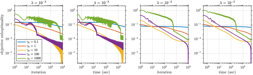
Figure S.4: Empirical performance of AdapTos for different choices of $\alpha$ for the overlapping group lasso problem with the hinge-loss. In this experiment we use RCV1 dataset (Lewis et al., 2004) ($n=677399$, $N=20242$) and tried two different values of the regularization parameter $\lambda=10^{-3}$ and $10^{-2}$.

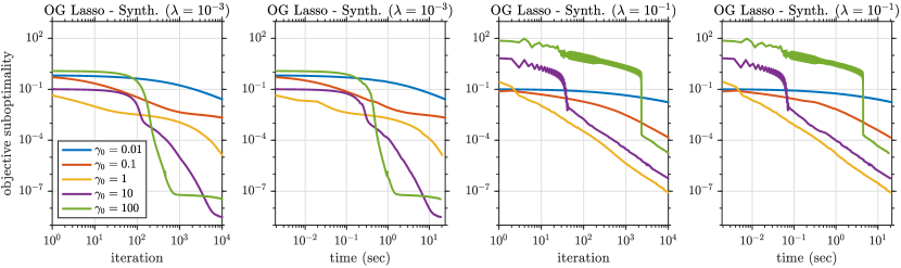
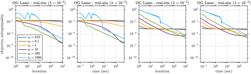
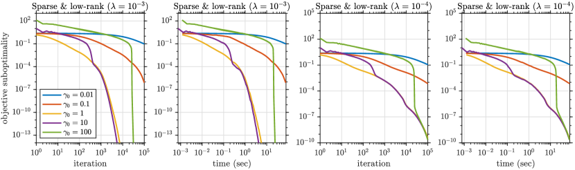
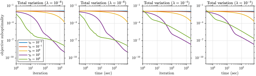
Figure S.5: Empirical performance of AdapTos with different choices of $\alpha$ for the problems with smooth and convex loss function studied in Section 6.1.

F.2 Details for Section 6.2

Figure S.7 shows the recovered approximations with $\ell_{1}$ and $\ell_{2}$-loss functions along with the original image and the noisy observation. $\ell_{1}$-loss is known to be more reliable against outliers, and it empirically generates a better approximation of the original image with 26.21 dB peak signal to noise ratio (PSNR) against 21.15 dB for the $\ell_{2}$-loss.

In Figure S.7 we extend the comparison in Figure 2 with the squared-$\ell_{2}$ loss.

$$\min_{\bm{X}\in\mathbb{R}^{m\times n}}\quad\frac{1}{2}\|\mathcal{A}(X)-Y\|_{2}^{2}\quad\text{subject to}\quad\|X\|_{\ast}\leq\lambda,~{}~{}~{}0\leq X\leq 1,$$ (S.94)

Note that the solution set is the same for $\ell_{2}$ and squared-$\ell_{2}$ formulations. However, squared-$\ell_{2}$ loss is smooth whereas $\ell_{2}$ loss is nonsmooth. Nevertheless, the empirical performance of AdapTos for the two formulations are similar. We also compare the evaluation of PSNR over the iterations. This comparison clearly demonstrates the advantage of using the robust $\ell_{1}$ loss formulation.

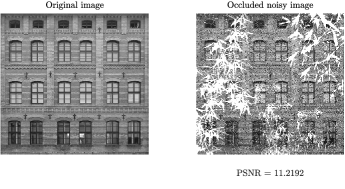
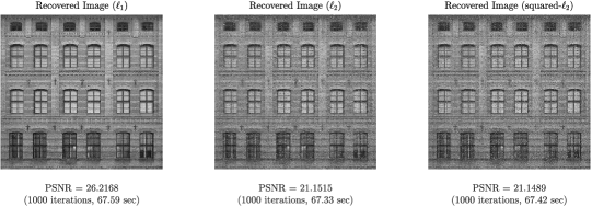
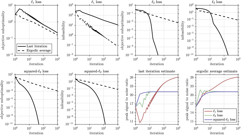
Figure S.6: Comparison or images recovered by minimizing the $\ell_{1}$, $\ell_{2}$ and squared-$\ell_{2}$ loss functions described in Section 6.2. $\ell_{1}$-loss empirically gives a better approximation with 5dB higher PSNR.

Figure S.7: Performance of AdapTos on image impainting problems with $\ell_{1}$, $\ell_{2}$, and squared-$\ell_{2}$ loss functions described in Section 6.2. The performance for nonsmooth $\ell_{2}$ loss and smooth squared-$\ell_{2}$ loss are qualitatively similar.

F.3 Details for Section 6.3

Let $\bm{y}=f(\bm{x},\bm{w})$ denote a generic deep neural network with $H$ hidden layers, which takes a vector input $x$ and returns a vector output $y$, and $w$ represents the column-vector concatenation of all adaptable parameters. $k$th hidden layer operates on input vector $\bm{\theta}_{k}$ and returns $\bm{\theta}_{k+1}$,

$$\bm{\theta}_{k+1} =\phi_{k}(\bm{W}_{k}\bm{\theta}_{k}+\bm{b}_{k}),\quad\text{for}~{}1\leq k\leq H,$$ (S.95)

where $\bm{\theta}_{1}=\bm{x}$ denotes the input layer by convention, $\{\bm{\theta}_{k},\bm{b}_{k}\}$ are the adaptable parameters of the layer and $\phi_{k}$ is an activation function to be applied entry-wise. We use ReLu activation (Glorot et al., 2011) for the hidden layers of the network and the softmax activation function for the output layer. We use the same initial weights as in (Scardapane et al., 2017), which is based on the method described in (Glorot & Bengio, 2010).

Given a set of $N$ training examples $\{(\bm{x}_{1},\bm{y}_{1}),\ldots,(\bm{x}_{N},\bm{y}_{N})\}$, we train the network by minimizing

$$\min_{\bm{w}\in\mathbb{R}^{n}}\quad\frac{1}{N}\sum_{i=1}^{N}L(\bm{y}_{i},f(\bm{x}_{i},\bm{w}))+\lambda\|\bm{w}\|_{1}+\lambda\sum_{\bm{\alpha}\in\Omega}\sqrt{|\bm{\alpha}|}\|\bm{\alpha}\|_{2},$$ (S.96)

with the standard cross-entropy loss given by $L(\bm{y},f(\bm{x},\bm{w}))=-\sum_{j=1}^{\mathrm{dim}(\bm{y})}y_{j}\log(f_{j}(\bm{x},\bm{w}))$. $\lambda>0$ is the regularization parameter. We set $\lambda=10^{-4}$, which is shown to provide the best results in terms of classification accuracy and sparsity in (Scardapane et al., 2017).

The first regularizer ($\ell_{1}$ penalty) in (S.96) promotes sparsity on the overall network, while the second regularizer (Group-Lasso penalty, introduced in (Yuan & Lin, 2006)) is used to achieve group-level sparsity. The goal is to force all outgoing connections from the same neurons to be simultaneously zero, so that we can safely remove them and obtain a compact network. To this end, $\Omega$ contains the sets of all outgoing connections from each neuron (corresponding to the rows of $\bm{W}_{k}$) and single element groups of bias terms (corresponding to the entries of $\bm{b}_{k}$).

We compare our methods against SGD, AdaGrad and Adam. We use minibatch size of $400$ for all methods. We use the built-in functions in Lasagne for SGD, AdaGrad and Adam. These methods use the subgradient of the overall objective (S.96). All of these methods have one learning rate parameter for tuning. We tune these parameters by trying the powers of $10$. We found that $\gamma_{0}=\alpha=1$ works well for TOS and AdapTos. For SGD and AdaGrad, we got the best performance when the learning rate parameter is set to $10^{-2}$, and for Adam we got the best results with $10^{-3}$.

Remark that subgradient methods are known to destroy sparsity at the intermediate iterations. For instance, the subgradients of $\ell_{1}$ norm are fully dense. In contrast, TOS and AdapTos handle the regularizers through their proximal operators. The advantage of using a proximal method instead of subgradients is outstanding. TOS and AdapTos result in precisely sparse networks whereas other methods can only get approximately sparse solutions. The comparison becomes especially stark in group sparsity, with no clear discontinuity in the spectrum for other methods.

Appendix G Additional Numerical Experiments

In this section, we present additional numerical experiments on isotonic regression and portfolio optimization problems. The experiments in this section are performed in Matlab R2018a with 2.6 GHz Quad-Core Intel Core i7 CPU.

G.1 Isotonic Regression

In this section, we compare the empirical performance of the adaptive step-size in Section 5 with the analytical step-size in Section 3. We consider the isotonic regression problem with the $\ell_{p}$-norm loss:

$$\min_{x\in\mathbb{R}^{n}}\quad\tfrac{1}{p}\|Ax-b\|_{p}^{p}\quad\mathrm{subject~{}to}\quad x_{1}\leq x_{2}\leq\ldots\leq x_{n},$$ (S.97)

where $A\in\mathbb{R}^{m\times n}$ is a given linear map and $b\in\mathbb{R}^{m}$ is the measurement vector. Projection onto the order constraint in (S.97) is challenging, but we can split it into two simpler constraints:

$$\min_{x\in\mathbb{R}^{n}}\quad\tfrac{1}{p}\|Ax-b\|_{p}^{p}\quad\mathrm{subject~{}to}\quad\left\{\begin{aligned} x_{1}\leq x_{2}\\ x_{3}\leq x_{4}\\[-5.0pt] \vdots\phantom{~{}~{}x_{1}}\end{aligned}\right\}~{}~{}~{}\mathrm{and}~{}~{}~{}\left\{\begin{aligned} x_{2}\leq x_{3}\\ x_{4}\leq x_{5}\\[-5.0pt] \vdots\phantom{~{}~{}x_{1}}\end{aligned}\right\}.$$ (S.98)

We demonstrate the numerical performance of the methods for various values of $p\in[1,2]$. Note that $p=1$ and $p=2$ capture the nonsmooth least absolute deviations loss and the smooth least squares loss respectively. For larger values of $p$, we expect AdapTos to exhibit faster rates by adapting to the underlying smoothness of the objective function.

We generate a synthetic test setup. To this end, we set the problem size as $m=100$ and $n=200$. We generate right and left singular vectors of $A$ by computing the singular value decomposition of a random matrix with iid entries drawn from the standard normal distribution. Then, we set the singular values according to a polynomial decay rule such that the $i$th singular vector is $1/i$. We generate $\smash{x^{\natural}\in\mathbb{R}^{n}}$ by sorting $n$ iid samples from the standard normal distribution. Then, we compute the noisy measurements $\smash{b=Ax^{\natural}+0.1\xi}$ where the entries of $\xi$ is drawn iid from the standard normal distribution.

By considering a decaying singular value spectrum for $A$ we control the condition number and make sure the problem is not very easy to solve. By adding noise, we ensure that the solution is not in the relative interior of the feasible set. Therefore, this experiment also supports our claim that AdapTos can achieve fast rates when the objective is smooth even if the solution does not lie in the interior of the feasible set.

When the problem is nonsmooth, i.e., when $p<2$, we use TOS with the analytical step-size in Section 3 and the adaptive step-size in Section 5. We choose $\alpha=\beta=\gamma_{0}=1$ without any tuning. When $p=2$, the problem is smooth so we also try TOS with the standard constant step-size $\gamma=1/L_{f}$ in this setting. We run each algorithm for $10^{5}$ iterations. In order to find the ground truth $f_{\star}$ we solve the problem to very high precision by using CVX (Grant & Boyd, 2014) with the SDPT3 solver (Toh et al., 1999).

We repeat the experiments with $20$ randomly generated data with different seeds and report the average performance in Figure S.8. This figure compares the performance we get by different step-size strategies in terms of objective suboptimality ($|f(z_{t})-f_{\star}|/f_{\star}$) and infeasbility bound ($\|z_{t}-x_{t}\|$). As expected, AdapTos performs better as $p$ becomes larger. Although it does not exactly match the performance of the fixed step-size $1/L_{f}$ when $f$ is smooth ($p=2$), remark that AdapTos does not require any prior knowledge on $L_{f}$ or $G_{f}$.

Figure S.8: Comparison of the empirical performance of TOS with the analytical step-size in Section 3 and the adaptive step-size in Section 5 on the isotonic regression problem in (S.97) with the $\ell_{p}$-loss function for various $p\in[1,2]$. For larger values of $p$, AdapTos exhibits faster convergence rates by adapting to the underlying smoothness of the objective function. For $p=2$, the problem is smooth so we also consider the standard fixed step-size $\gamma=1/L_{f}$ in this setting. Solid lines represent the last iteration and the dashed lines correspond to the ergodic sequences $\bar{x}_{t}$ and $\bar{z}_{t}$.

G.2 Portfolio Optimization

In this section, we demonstrate the advantage of stochastic methods for machine learning problems. We consider the portfolio optimization with empirical risk minimization from Section 5.1 in (Yurtsever et al., 2016):

$$\min_{x\in\mathbb{R}^{n}}\quad\frac{1}{2}\sum_{i=1}^{N}|\langle a_{i},x\rangle-b|^{2}\quad\mathrm{subject~{}to}\quad x\in\Delta\quad\text{and}\quad\langle a_{\mathrm{av}},x\rangle\geq b$$ (S.99)

where $\Delta$ is the unit simplex. Here $n$ is the number of different assets and $x\in\Delta$ represents a portfolio. The collection of $\{a_{i}\}_{i=1}^{N}$ represents the returns of each asset at different time instances, and the $a_{\mathrm{av}}$ is the average returns for each asset that is assumed to be known or estimated. Given a minimum target return $b\in\mathbb{R}$, the goal is to reduce the risk by minimizing the variance. As in (Yurtsever et al., 2016), we set the target return as the average return over all assets, i.e., $b=\mathrm{mean}(a_{\mathrm{av}})$.

In addition, we also consider a modification of (S.99) with the least absolute deviation loss, which is nonsmooth but known to be more robust against outliers:

$$\min_{x\in\mathbb{R}^{n}}\quad\sum_{i=1}^{N}|\langle a_{i},x\rangle-b|\quad\mathrm{subject~{}to}\quad x\in\Delta\quad\text{and}\quad\langle a_{\mathrm{av}},x\rangle\geq b.$$ (S.100)

We use $4$ different real portfolio datasets: Dow Jones industrial average (DJIA, 30 stocks for 507 days), New York stock exchange (NYSE, 36 stocks for 5651 days), Standard & Poor’s 500 (SP500, 25 stocks for 1276 days), and Toronto stock exchange (TSE, 88 stocks for 1258 days).

For both problems and each dataset, we run AdapTos with full (sub)gradients and stochastic (sub)gradients and compare their performances. We choose $\alpha=\beta=1$ without tuning and run the algorithms for $10$ epochs. In the stochastic setting, we evaluate a (sub)gradient estimator from a single datapoint chosen uniformly at random with replacement at every iteration. We run the stochastic algorithm 20 times with different random seeds and present the average performance. To find the ground truth $f_{\star}$ we solve the problems to very high precision by using CVX (Grant & Boyd, 2014) with the SDPT3 solver (Toh et al., 1999). Figures S.10 and S.10 present the results of this experiment for (S.99) and (S.100) respectively.

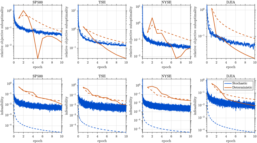
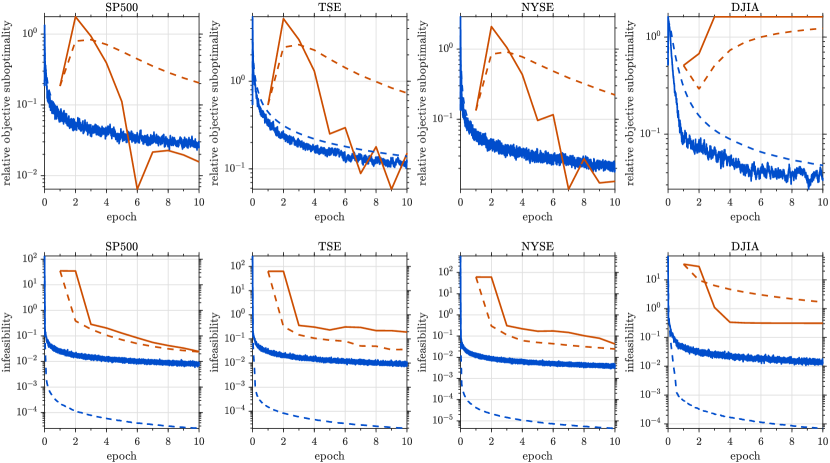
Figure S.9: Comparison of AdapTos with stochastic and deterministic gradients on the smooth portfolio optimization problem with least-squares loss in (S.99) for four different datasets. Solid and dashed lines represent the last and ergodic iterates respectively.

Figure S.10: Comparison AdapTos with stochastic and deterministic gradients on the nonsmooth portfolio optimization problem with least absolute deviations loss in (S.100) for four different datasets. Solid and dashed lines represent the last and ergodic iterates respectively.

References

- Azadi & Sra (2014) Azadi, S. and Sra, S. Towards an optimal stochastic alternating direction method of multipliers. In International Conference on Machine Learning, pp. 620–628. PMLR, 2014.
- Bach & Levy (2019) Bach, F. and Levy, K. Y. A universal algorithm for variational inequalities adaptive to smoothness and noise. In Conference on Learning Theory, pp. 164–194. PMLR, 2019.
- Barbero & Sra (2018) Barbero, A. and Sra, S. Modular proximal optimization for multidimensional total-variation regularization. The Journal of Machine Learning Research, 19(1):2232–2313, 2018.
- Bauschke et al. (2011) Bauschke, H. H., Combettes, P. L., et al. Convex analysis and monotone operator theory in Hilbert spaces, volume 408. Springer, 2011.
- Blalock et al. (2020) Blalock, D., Ortiz, J. J. G., Frankle, J., and Guttag, J. What is the state of neural network pruning? arXiv preprint arXiv:2003.03033, 2020.
- Briceño-Arias (2015) Briceño-Arias, L. M. Forward-douglas–rachford splitting and forward-partial inverse method for solving monotone inclusions. Optimization, 64(5):1239–1261, 2015.
- Cevher et al. (2018) Cevher, V., Vũ, B. C., and Yurtsever, A. Stochastic forward douglas-rachford splitting method for monotone inclusions. In Large-Scale and Distributed Optimization, pp. 149–179. Springer, 2018.
- Chambolle & Pock (2016) Chambolle, A. and Pock, T. On the ergodic convergence rates of a first-order primal–dual algorithm. Mathematical Programming, 159(1):253–287, 2016.
- Chang & Lin (2011) Chang, C.-C. and Lin, C.-J. Libsvm: A library for support vector machines. ACM transactions on intelligent systems and technology (TIST), 2(3):1–27, 2011.
- Condat (2013) Condat, L. A primal–dual splitting method for convex optimization involving lipschitzian, proximable and linear composite terms. Journal of optimization theory and applications, 158(2):460–479, 2013.
- Cutkosky (2019) Cutkosky, A. Anytime online-to-batch, optimism and acceleration. In International Conference on Machine Learning, pp. 1446–1454. PMLR, 2019.
- Davis & Yin (2017) Davis, D. and Yin, W. A three-operator splitting scheme and its optimization applications. Set-valued and variational analysis, 25(4):829–858, 2017.
- Ding et al. (2019) Ding, L., Yurtsever, A., Cevher, V., Tropp, J. A., and Udell, M. An optimal-storage approach to semidefinite programming using approximate complementarity. arXiv preprint arXiv:1902.03373, 2019.
- Duchi et al. (2011) Duchi, J., Hazan, E., and Singer, Y. Adaptive subgradient methods for online learning and stochastic optimization. Journal of machine learning research, 12(7), 2011.
- El Halabi & Cevher (2015) El Halabi, M. and Cevher, V. A totally unimodular view of structured sparsity. In Artificial Intelligence and Statistics, pp. 223–231. PMLR, 2015.
- Glorot & Bengio (2010) Glorot, X. and Bengio, Y. Understanding the difficulty of training deep feedforward neural networks. In Proceedings of the thirteenth international conference on artificial intelligence and statistics, pp. 249–256. JMLR Workshop and Conference Proceedings, 2010.
- Glorot et al. (2011) Glorot, X., Bordes, A., and Bengio, Y. Deep sparse rectifier neural networks. In Proceedings of the fourteenth international conference on artificial intelligence and statistics, pp. 315–323. JMLR Workshop and Conference Proceedings, 2011.
- Grant & Boyd (2014) Grant, M. and Boyd, S. CVX: Matlab software for disciplined convex programming, version 2.1, 2014.
- He et al. (2016) He, K., Zhang, X., Ren, S., and Sun, J. Deep residual learning for image recognition. In Proceedings of the IEEE conference on computer vision and pattern recognition, pp. 770–778, 2016.
- Higham & Strabić (2016) Higham, N. J. and Strabić, N. Anderson acceleration of the alternating projections method for computing the nearest correlation matrix. Numerical Algorithms, 72(4):1021–1042, 2016.
- Hoffmann (1992) Hoffmann, A. The distance to the intersection of two convex sets expressed by the distances to each of them. Mathematische Nachrichten, 157(1):81–98, 1992.
- Kavis et al. (2019) Kavis, A., Levy, K. Y., Bach, F., and Cevher, V. Unixgrad: A universal, adaptive algorithm with optimal guarantees for constrained optimization. In Proceedings of the 33rd International Conference on Neural Information Processing Systems, 2019.
- Kundu et al. (2018) Kundu, A., Bach, F., and Bhattacharya, C. Convex optimization over intersection of simple sets: improved convergence rate guarantees via an exact penalty approach. In International Conference on Artificial Intelligence and Statistics, pp. 958–967. PMLR, 2018.
- LeCun (1998) LeCun, Y. The mnist database of handwritten digits. http://yann. lecun. com/exdb/mnist/, 1998.
- Levy (2017) Levy, K. Y. Online to offline conversions, universality and adaptive minibatch sizes. In Proceedings of the 31st International Conference on Neural Information Processing Systems, 2017.
- Levy et al. (2018) Levy, K. Y., Yurtsever, A., and Cevher, V. Online adaptive methods, universality and acceleration. In Proceedings of the 32nd International Conference on Neural Information Processing Systems, 2018.
- Lewis et al. (2004) Lewis, D. D., Yang, Y., Russell-Rose, T., and Li, F. Rcv1: A new benchmark collection for text categorization research. Journal of machine learning research, 5(Apr):361–397, 2004.
- Malitsky & Pock (2018) Malitsky, Y. and Pock, T. A first-order primal-dual algorithm with linesearch. SIAM Journal on Optimization, 28(1):411–432, 2018.
- Mishchenko & Richtárik (2019) Mishchenko, K. and Richtárik, P. A stochastic decoupling method for minimizing the sum of smooth and non-smooth functions. arXiv preprint arXiv:1905.11535, 2019.
- Nesterov (2003) Nesterov, Y. Introductory lectures on convex optimization: A basic course, volume 87. Springer Science & Business Media, 2003.
- Nesterov (2015) Nesterov, Y. Universal gradient methods for convex optimization problems. Mathematical Programming, 152(1):381–404, 2015.
- Ouyang et al. (2013) Ouyang, H., He, N., Tran, L., and Gray, A. Stochastic alternating direction method of multipliers. In International Conference on Machine Learning, pp. 80–88. PMLR, 2013.
- Pedregosa (2016) Pedregosa, F. On the convergence rate of the three operator splitting scheme. arXiv preprint arXiv:1610.07830, 2016.
- Pedregosa & Gidel (2018) Pedregosa, F. and Gidel, G. Adaptive three operator splitting. In International Conference on Machine Learning, pp. 4085–4094, 2018.
- Pedregosa et al. (2019) Pedregosa, F., Fatras, K., and Casotto, M. Proximal splitting meets variance reduction. In The 22nd International Conference on Artificial Intelligence and Statistics, pp. 1–10. PMLR, 2019.
- Pedregosa et al. (2020) Pedregosa, F., Negiar, G., and Dresdner, G. copt: composite optimization in python. 2020. doi: 10.5281/zenodo.1283339. URL http://openo.pt/copt/.
- Raguet et al. (2013) Raguet, H., Fadili, J., and Peyré, G. A generalized forward-backward splitting. SIAM Journal on Imaging Sciences, 6(3):1199–1226, 2013.
- Rakhlin & Sridharan (2013) Rakhlin, A. and Sridharan, K. Optimization, learning, and games with predictable sequences. In Proceedings of the 26th International Conference on Neural Information Processing Systems-Volume 2, pp. 3066–3074, 2013.
- Salim et al. (2020) Salim, A., Condat, L., Mishchenko, K., and Richtárik, P. Dualize, split, randomize: Fast nonsmooth optimization algorithms. arXiv preprint arXiv:2004.02635, 2020.
- Scardapane et al. (2017) Scardapane, S., Comminiello, D., Hussain, A., and Uncini, A. Group sparse regularization for deep neural networks. Neurocomputing, 241:81–89, 2017.
- Shivanna et al. (2015) Shivanna, R., Chatterjee, B., Sankaran, R., Bhattacharyya, C., and Bach, F. Spectral norm regularization of orthonormal representations for graph transduction. In Neural Information Processing Systems, 2015.
- Tibshirani et al. (2011) Tibshirani, R. J., Hoefling, H., and Tibshirani, R. Nearly-isotonic regression. Technometrics, 53(1):54–61, 2011.
- Toh et al. (1999) Toh, K.-C., Todd, M. J., and Tütüncü, R. H. SDPT3—a MATLAB software package for semidefinite programming, version 1.3. Optimization methods and software, 11(1-4):545–581, 1999.
- Vũ (2013) Vũ, B. C. A splitting algorithm for dual monotone inclusions involving cocoercive operators. Advances in Computational Mathematics, 38(3):667–681, 2013.
- Yan (2018) Yan, M. A new primal–dual algorithm for minimizing the sum of three functions with a linear operator. Journal of Scientific Computing, 76(3):1698–1717, 2018.
- Yuan et al. (2011) Yuan, L., Liu, J., and Ye, J. Efficient methods for overlapping group lasso. Advances in neural information processing systems, 24:352–360, 2011.
- Yuan & Lin (2006) Yuan, M. and Lin, Y. Model selection and estimation in regression with grouped variables. Journal of the Royal Statistical Society: Series B (Statistical Methodology), 68(1):49–67, 2006.
- Yurtsever et al. (2016) Yurtsever, A., Vũ, B. C., and Cevher, V. Stochastic three-composite convex minimization. In Proceedings of the 30th International Conference on Neural Information Processing Systems, pp. 4329–4337, 2016.
- Yurtsever et al. (2018) Yurtsever, A., Fercoq, O., Locatello, F., and Cevher, V. A conditional gradient framework for composite convex minimization with applications to semidefinite programming. In International Conference on Machine Learning, pp. 5727–5736. PMLR, 2018.
- Yurtsever et al. (2021) Yurtsever, A., Mangalick, V., and Sra, S. Three operator splitting with a nonconvex loss function. In International Conference on Machine Learning, pp. 12267–12277. PMLR, 2021.
- Zeng & So (2018) Zeng, W.-J. and So, H. C. Outlier–robust matrix completion via -minimization. IEEE Trans. on Sig. Process, 66(5):1125–1140, 2018.
- Zhao & Cevher (2018) Zhao, R. and Cevher, V. Stochastic three-composite convex minimization with a linear operator. In International Conference on Artificial Intelligence and Statistics, pp. 765–774. PMLR, 2018.
- Zhao et al. (2019) Zhao, R., Haskell, W. B., and Tan, V. Y. An optimal algorithm for stochastic three-composite optimization. In The 22nd International Conference on Artificial Intelligence and Statistics, pp. 428–437. PMLR, 2019.