Numerical Simulations of Convective 3-Dimensional Red Supergiant Envelopes

Abstract

We explore the three-dimensional properties of convective, luminous ($L\approx 10^{4.5}-10^{5}L_{\odot}$), Hydrogen-rich envelopes of Red Supergiants (RSGs) based on radiation hydrodynamic simulations in spherical geometry using Athena++. These computations comprise $\approx 30\%$ of the stellar volume, include gas and radiation pressure, and self-consistently track the gravitational potential for the outer $\approx 3M_{\odot}$ of the simulated $M\approx 15M_{\odot}$ stars. This work reveals a radius, $R_{\mathrm{corr}}$, around which the nature of the convection changes. For $r>R_{\mathrm{corr}}$, though still optically thick, diffusion of photons dominates the energy transport. Such a regime is well-studied in less luminous stars, but in RSGs, the near- (or above-) Eddington luminosity (due to opacity enhancements at ionization transitions) leads to the unusual outcome of denser regions moving outwards rather than inward. This region of the star also has a large amount of turbulent pressure, yielding a density structure much more extended than 1D stellar evolution predicts. This “halo” of material will impact predictions for both shock breakout and early lightcurves of Type II-P supernovae. Inside of $R_{\mathrm{corr}}$, we find a nearly flat entropy profile as expected in the efficient regime of mixing-length-theory (MLT). Radiation pressure provides $\approx 1/3$ of the support against gravity in this region. Our comparisons to MLT suggest a mixing length of $\alpha=3-4$, consistent with the sizes of convective plumes seen in the simulations. The temporal variability of these 3D models is mostly on the timescale of the convective plume lifetimes ($\approx 300$ days), with amplitudes consistent with those observed photometrically.

1 Introduction

As massive ($M\mathrel{\vbox{ \offinterlineskip\halign{\hfil$#$\cr>\cr\kern 2.0pt\cr\sim\cr\kern-2.0pt\cr}}}10M_{\odot}$) stars leave the main sequence, they expand to become Red Supergiants (RSGs), reaching radii of $\approx 300-1200R_{\odot}$ and luminosities of $\approx 10^{4}-10^{5.5}L_{\odot}$ (e.g. Levesque et al., 2006; Drout et al., 2012; Massey et al., 2021), approaching the Eddington limit and receiving increasing hydrostatic support from radiation pressure. These stars are characterized by low-density convective hydrogen-rich envelopes with large scale heights ($H/r\approx 0.3$) and sonic convection near their surfaces. They are intrinsically variable and pulsate in large-amplitude coherent modes (e.g. Kiss et al. 2006; Soraisam et al. 2018; Chatys et al. 2019; Ren et al. 2019; Dorn-Wallenstein et al. 2020) and their 3D nature is revealed to us in spectro-interferometric observations of nearby stars (e.g. Arroyo-Torres et al. 2015; Kravchenko et al. 2019, 2021; Montargès et al. 2021; Norris et al. 2021).

It is a theoretical challenge to realistically model stars, or even parts of stars, in 3D. This is especially true when radiative transfer must also be simultaneously solved through a highly turbulent medium with large density variations over optical depths ranging from far above unity down to the radiating photosphere. This radiation hydrodynamic (RHD) challenge has been very well-addressed in cases where this region is close to plane-parallel, starting with the fundamental work for the Sun (Stein & Nordlund, 1989, 1998), and now ranging across the HR diagram (e.g. Trampedach et al., 2013, 2014a, 2014b; Magic et al., 2013a, b, 2015; Chiavassa et al., 2018a; Sonoi et al., 2019), building on earlier 2D RHD work (see Ludwig et al. 1999 for an excellent summary). These 3D computations have yielded a physical understanding of the nature of RHD convection in this limit, and provide a quantitative ability to set the outer boundary condition in 1D stellar models (e.g. Trampedach et al., 2014a; Salaris & Cassisi, 2015; Magic, 2016; Mosumgaard et al., 2018; Spada et al., 2021) for $\log g\mathrel{\vbox{ \offinterlineskip\halign{\hfil$#$\cr>\cr\kern 2.0pt\cr\sim\cr\kern-2.0pt\cr}}}1.5$, including for asteroseismic applications (Mosumgaard et al., 2020). While we have detailed understanding of the outer layers and quantitative surface relations for more compact, less luminous stars as guided by these works, such clarity has not been reached where the region requiring RHD calculations necessitates spherical geometry to capture large-scale plumes, and where the luminosity is locally super-Eddington.

In fainter giants, some of these aspects have been further addressed with global 3D simulations. In Red Giant Branch (RGB) stars, simulations of the convective interior reveal relatively flat velocity profiles set by large-scale convective plumes, and large temperature and density fluctuations (Brun & Palacios, 2009). These large-scale plumes extend up through the photosphere and produce granulation effects which can be interpreted by comparison of 3D models to interferometric data (e.g. Chiavassa et al., 2010a, 2017). In Asymptotic Giant Branch (AGB) stars, 3D simulations have revealed additional insights about the pulsational and circumstellar structure, with nearly-spherical shock fronts from large-scale convective cells which also levitate material to radii at which they can form dust (e.g. Freytag & Höfner, 2008; Freytag et al., 2017). These simulations can then be used to, e.g., generate inner boundary conditions for 1D wind models (Liljegren et al., 2018), and interpret both interferometric and photometric observations (e.g. Chiavassa et al., 2018b, 2020).

In the luminous RSG regime, early simulations focused on surface turbulence and magnetic properties (e.g. Freytag et al. 2002; Dorch 2004). Further simulations have been used to provide limb darkening coefficients and confirm the presence of large convective cells from interferometric observations of Betelgeuse (Chiavassa et al., 2009, 2010b). Chiavassa et al. (2011b) provide photocentric noise models towards quantifying Gaia astrometric parallax uncertainties and explain the “cosmic noise” impacting Hipparcos photometric measurements of Betelgeuse and Antares, while Chiavassa et al. (2011a) characterize microturbulence and macroturbulence parameters in grey- and frequency-dependent RSG atmosphere simulations. Further predictions from these models have been made with radiation transfer post-processing with the software OPTIM3D (Plez & Chiavassa, 2013) and reveal the inability to define a single “surface” responsible for setting the effective temperature, $T_{\mathrm{eff}}$.

A unifying feature of theory and observations of RSGs is the turbulent, extended outer envelope which manifests these inherently 3D convective properties. In 1D stellar evolution models, convection is conventionally handled by the Mixing Length Theory (MLT). The MLT approach derives from considering the fate of fluid elements as they move vertically a distance referred to as the mixing length $\ell\equiv\alpha H$, where $\alpha$ is a free parameter which can be calibrated to observations or by 3D simulations (Böhm-Vitense, 1958; Henyey et al., 1965; Cox & Giuli, 1968). Especially in Red Giants and Supergiants, mixing length assumptions, especially the value of $\alpha$ (and assumptions relevant to the structure and location of convective boundaries, which we will not explore in this work) strongly influence the stellar radii and $T_{\mathrm{eff}}$ (e.g. Stothers & Chin, 1995; Meynet & Maeder, 1997; Massey & Olsen, 2003; Meynet et al., 2015). While empirical constraints are useful, even crucial, for producing RSG models which match observed stars in luminosity, $L$, and $T_{\mathrm{eff}}$ (e.g. Chun et al., 2018), a first-principles calibration of MLT to 3D simulations of RSG envelopes remains an open channel for theoretical progress in characterizing the nature of convection in these very luminous objects.

The turbulent RSG envelope also plays a crucial role at the end of the star’s life, as a strong shock emerges from the collapsed core and propagates rapidly through the envelope. Such explosions result in Type II-P SNe with $\simeq\!100$-day plateaus in their lightcurves whose properties depend on the envelope structure, and especially the progenitor radius, ejected mass, explosion energy and ⁵⁶Ni mass (e.g. Popov 1993; Kasen & Woosley 2009; Sukhbold et al. 2016). The exact initial mass range of stars exploding as Type II-Ps is still a matter of significant debate (the so-called “RSG problem”, e.g. Smartt, 2009, 2015; Davies & Beasor, 2018; Kochanek, 2020; Davies & Beasor, 2020a, b). If the RSG radius is known at the moment of explosion, then light curve modeling can be used to constrain the ejected mass (Goldberg et al., 2019; Martinez & Bersten, 2019; Goldberg & Bildsten, 2020), with some sensitivity to the pulsation mode and phase at the time of explosion (see discussion in Goldberg et al. 2020). However, if the progenitor radius is unknown, very different stellar properties can yield identical lightcurves and photospheric velocities after the first $\approx 30$ days (Dessart & Hillier, 2019; Goldberg et al., 2019), limiting our ability to infer masses and explosion energies solely from these observations.

Early Supernova observations can assist with breaking these degeneracies, but doing so is hampered by our lack of understanding of the density structure of the outermost RSG layers responsible for the early time emission (see, e.g. Morozova et al., 2016). In addition, Type II-P SNe frequently exhibit luminosities in excess of explosion models that assume a simple stellar photosphere (e.g. Morozova et al. 2017, 2018). This early excess is often attributed to interaction between the SN ejecta and the progenitor’s outgoing wind (e.g. Moriya et al., 2018) or ejecta from pre-SN outbursts (Fuller, 2017; Morozova et al., 2020), and poses challenge in cleanly interpreting these early phases of SN evolution (see, e.g. Hosseinzadeh et al., 2018). It is also possible that these discrepancies are because the density structure in the vicinity of the photosphere is simply not well-described by conventional 1D stellar models. One important long-term goal of our effort is to better constrain the role of the 3D gas distribution in early SN emission.

This paper is organized as follows: In §2, we describe motivating expectations for the 3D regime we aim to explore, making use of Modules for Experiments in Stellar Astrophysics (MESA Paxton et al., 2011, 2013, 2015, 2018, 2019) to illustrate the importance of a proper 3D treatment of RSG envelopes. In §3 we describe our 3D Athena++ (Stone et al., 2020) RHD setup for RSG envelopes, and in §4 we discuss the convective properties of these envelopes, comparing where possible to findings of earlier 3D RSG models. We then compare our 3D envelope models to predictions from MLT where appropriate (§5). Finally, we discuss our results and comment on future directions in §6.

2 Properties of 1D Red Supergiant Models and Open Challenges

For our initial exploration, we constructed a suite of solar-metallicity ($Z=0.02$) models in MESA, following the test suite case make_pre_ccsn_IIp in revision 15140, shown in Fig. 1 from the onset of core H burning through the end of core Si burning. Our fiducial non-rotating models have modest exponential overshoot with overshooting parameter $f_{\mathrm{ov}}=0.016$, a wind efficiency of $\eta_{\mathrm{wind}}=0.2$ using the 'Dutch' scheme in MESA (Nugis & Lamers, 2000; Vink et al., 2001; Glebbeek et al., 2009), core mixing length $\alpha_{\mathrm{c}}=1.5$ in regions where the H fraction $X_{\mathrm{H}}\leq 0.5$, and mixing length $\alpha_{\mathrm{H}}=3$ in the H-rich envelope ($X_{\mathrm{H}}>0.5$). These parameters were chosen to be similar to those of the Type IIP Supernova progenitor models in Paxton et al. (2018), motivated also by the findings of Farmer et al. (2016).

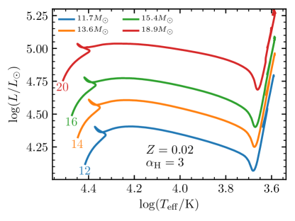
Figure 1: H-R diagrams of non-rotating MESA models with initial masses of $M_{i}/M_{\odot}$=12 (blue), 14 (orange), 16 (green), and 20 (red), from the main sequence through core Si burning. Final masses are given in the legend.

The left panels of Figure 2 show the structure of four model RSG envelopes at the end of core C burning (central $X_{\mathrm{C}}<10^{-6}$) with initial masses ranging from 12 to 20 $M_{\odot}$. The x-axis excludes the He core, which is always inside of $r=10R_{\odot}$ for all models. Through the envelope, the density falls by 3-4 orders of magnitude, nearly matching $\rho\propto 1/r^{2}$ through most of the inner envelope. The pressure scale height, $H=P/\rho g$, is large due to the weak gravity in the envelope, with $H/r\approx 0.3$ even at the half-radius coordinate. The envelope is fully convective, and both radiation pressure and gas pressure contribute significantly to the total pressure, with gas pressure dominating near the surface. Additionally, the opacity is very large throughout the envelope, dominated by opacity peaks from H and He ionization transitions inside the convective region.

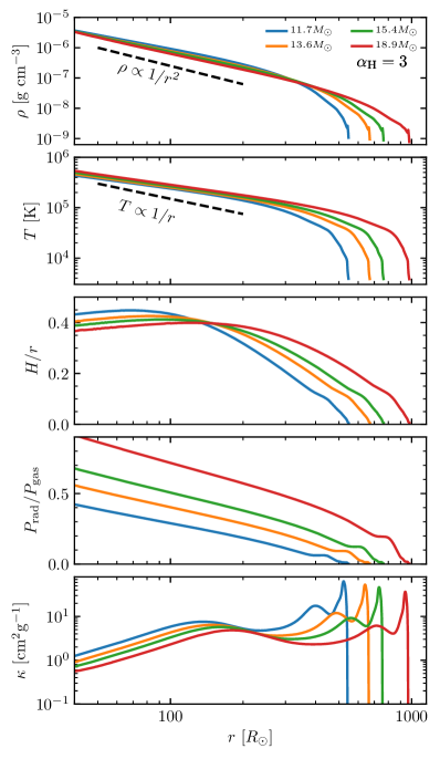
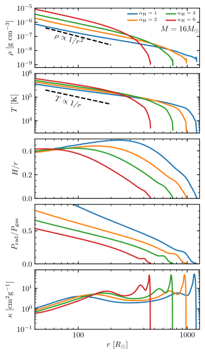
Figure 2: Top to bottom: Density, temperature, pressure scale height divided by radius, radiation to gas pressure ratio, and opacity as a function of radial coordinate $r$ in $Z=0.02$ RSG models. Left: Initial masses of $M_{i}/M_{\odot}$=12 (blue), 14 (orange), 16 (green), and 20 (red), all with $\alpha_{\mathrm{H}}=3$. Right: Masses of $M=16M_{\odot}$, varying the mixing length in the Hydrogen-rich envelope, $\alpha_{\mathrm{H}}$, for $\alpha_{\mathrm{H}}=1$ (blue), $\alpha_{\mathrm{H}}=2$ (orange), $\alpha_{\mathrm{H}}=3$ (green), and $\alpha_{\mathrm{H}}=6$ (red); here winds were neglected to isolate the effects of varying $\alpha_{\mathrm{H}}$, leading to the slight differences between the green lines in the left and right panels.

Where convection is “efficient”, $\nabla$ is nearly $\nabla_{\mathrm{e}}\approx\nabla_{\mathrm{ad}}$ and the fluid structure follows the adiabat. There are two senses in which convection is said to be inefficient. When the convection is inefficient in the superadiabatic sense (i.e. $\nabla\gg\nabla_{\mathrm{e}}$, where $\nabla=d\ln{T}/d\ln{P}$ and $\nabla_{\mathrm{e}}$ is the internal $\nabla$ of a convective parcel; see Table 2 in Appendix B), a rising fluid element will be hotter than the surrounding medium, and it will accelerate as it moves outwards in order to carry the flux. The stellar entropy profile thus declines. The convection can also be inefficient in the radiative sense, or “lossy”, when a convective fluid parcel has sufficient time to radiate its internal energy to the cooler surrounding as it rises. In a medium with $P_{\mathrm{gas}}\gg P_{\mathrm{rad}}$, the optical depth at which radiation is able to contribute significantly to the energy transport and lossy convection is expected is $\tau<\tau_{\mathrm{crit}}$, where

$$\tau_{\mathrm{crit}}\approx\frac{P_{\mathrm{rad}}}{P_{\mathrm{gas}}}\frac{c}{v_{c}},$$ (1)

where $c$ is the speed of light, and $v_{c}$ is the radial component of the convective velocity. The factor of $P_{\mathrm{rad}}/P_{\mathrm{gas}}$ comes from the fact that in the gas-pressure-dominated region near the cool stellar surface the parcel must evacuate the radiation field $P_{\mathrm{rad}}/P_{\mathrm{gas}}$ times in order to carry the same flux by radiation as convection (Kippenhahn et al., 2013). For $\tau>\tau_{\mathrm{crit}}$ where a parcel is unable to lose heat to radiation, $\nabla_{\mathrm{e}}\approx\nabla_{\mathrm{ad}}$. We will note later, in §4.4, the close relationship between $\tau/\tau_{\mathrm{crit}}$ and the more commonly-discussed convective efficiency parameter, $\gamma$.

In MLT, $\nabla-\nabla_{\mathrm{e}}$ is directly related to the mixing length $\ell=\alpha H$ by (Kippenhahn et al., 2013)

$$F_{\mathrm{conv}}=\rho c_{P}T\sqrt{gQ}\frac{\ell^{2}}{\sqrt{\nu}}H^{-3/2}(\nabla-\nabla_{\mathrm{e}})^{3/2},$$ (2)

where $F_{\mathrm{conv}}$ is the flux carried by convection, $Q=-\mathrm{D}\ln T/\mathrm{D}\ln\rho=(4-3\beta_{P})/\beta_{P}$ where $\beta_{P}=P_{\mathrm{gas}}/(P_{\mathrm{rad}}+P_{\mathrm{gas}})$ for an equation of state (EOS) made up of radiation and gas, $\nu=8$ following Henyey et al. (1965) and others, and $c_{P}$ is the specific heat at constant pressure.

So as to explore the dependence of the RSG envelope structure on the mixing length $\alpha_{\mathrm{H}}$, we constructed additional 16$M_{\odot}$ RSG models varying $\alpha_{H}$ from 1 to 6. In these, we neglect mass loss due to winds ($\eta_{\mathrm{wind}}=0.0$) and vary $\alpha_{\mathrm{H}}$ away from the fiducial value of $\alpha_{\mathrm{H}}=3$ only at the end of core He burning in order to ensure that the resulting models have comparable core masses, $M_{\mathrm{c,He}}=5.2M_{\odot}$, and luminosities, $\log(L/L_{\odot})=5.06$. The structure of these models is shown in the right panels of Figure 2. Lower values of $\alpha_{\mathrm{H}}$ produce models with larger radii, lower densities, and lower temperatures throughout the envelope.

The upper panels of Fig. 3 show the specific entropy, $s$, profiles for models varying the initial mass (left) and $\alpha_{\mathrm{H}}$ (right) at the end of core C burning. The lower panels compare $\tau_{\mathrm{crit}}$ (dashed lines) to the optical depth $\tau$ (solid lines). The transition to lossy convection with radiation-dominated transport typically occurs around $T\approx 10^{4}$K and $\tau=\tau_{\mathrm{crit}}\approx 300$, which is near the H opacity peak seen in Fig. 2. At that location, the peak in opacity and large luminosity implies $L\gg L_{\mathrm{Edd}}$ there, a critical distinction for RSG models compared to main-sequence, RGB, or AGB stars. As $T$ approaches $T_{\mathrm{eff}}$, $v_{c}$ declines to zero in a very thin radiative region above the convection zone. The green models are comparable between the left and right panels, with the only substantive difference being the inclusion of mass loss in the left panel leading to a slightly lower core mass, $M_{\mathrm{c,He}}=4.9M_{\odot}$, and luminosity, $\log(L/L_{\odot})=5.02$.

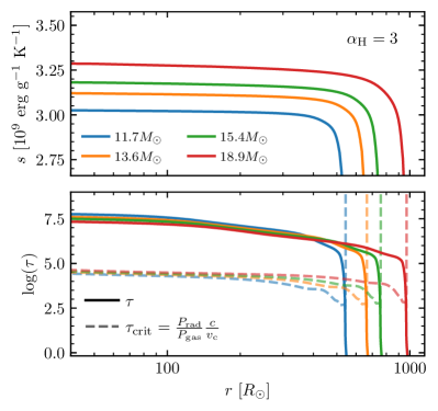
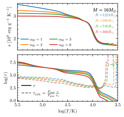
Figure 3: Specific entropy (upper panels) and optical depths (lower panels) for RSG models of different initial mass and $\alpha_{\mathrm{H}}=3$ (left panels), and varying $\alpha_{\mathrm{H}}$ with $M=16M_{\odot}$ (right panels). The optical depth remains much higher than $\tau_{\mathrm{crit}}$ (dashed lines) until $\tau\approx 300$ near $T\approx 10^{4}$ K.

Varying initial mass increases the luminosity and thereby $s$, with relatively flat entropy profiles that begin to decline near the surface. Decreasing $\alpha_{\mathrm{H}}$ decreases the efficiency of the convection, causing a steeper temperature gradient and an entropy decline. Larger mixing lengths correspond to more efficient convection and produce higher $T_{\mathrm{eff}}$. For a given luminosity, this leads to different radii with varying $\alpha_{\mathrm{H}}$, from $R=460R_{\odot}$ when $\alpha_{\mathrm{H}}=6$ to $R=1223R_{\odot}$ when $\alpha_{\mathrm{H}}=1$, despite comparable envelope masses and luminosities.

The assumed mixing length thus plays a dual role in determining the stellar structure. Foremost, the entropy profile declines even where $\tau\gg\tau_{\mathrm{crit}}$, especially for lower $\alpha_{\mathrm{H}}$, suggesting true superadiabatic convection with nonnegligible $\nabla-\nabla_{\mathrm{e}}$. The choice of $\alpha_{\mathrm{H}}$ influences $\nabla-\nabla_{\mathrm{e}}$ via Eq. (2) for a given $F_{\mathrm{conv}}$, and therefore determines the deviation of the temperature profile from the adiabat. Secondly, $\alpha_{\mathrm{H}}$ determines the adiabat on which the envelope sits. This effect can also be seen in models of cool stars more generally (e.g. Stothers & Chin, 1995; Meynet & Maeder, 1997; Massey & Olsen, 2003; Meynet et al., 2015) and is pronounced where convection occurs over orders of magnitude in radius, such as in cool giants. Running a further suite of models where we varied the location where the mixing length coefficient changes from a fixed $\alpha_{\mathrm{c}}$=1.5 to variable $\alpha_{\mathrm{H}}$ at different temperature coordinates, rather than setting the transition to be at the H-He interface as in our fiducial models, we find that changing $\alpha_{\mathrm{H}}$ in the lossy outer envelope below a few times $10^{4}$K (where $\tau\mathrel{\vbox{ \offinterlineskip\halign{\hfil$#$\cr<\cr\kern 2.0pt\cr\sim\cr\kern-2.0pt\cr}}}\tau_{\mathrm{crit}}$) is what primarily determines the outer radius of the star, as the entropy decline in that region is fixed (as seen in the upper right panel of Fig. 3). Since $\rho\mathrel{\vbox{ \offinterlineskip\halign{\hfil$#$\cr\propto\cr\kern 2.0pt\cr\sim\cr\kern-2.0pt\cr}}}1/r^{2}$, the stellar radius determines the density at the base of the envelope, the radiation to gas pressure ratio, the entropy, and thereby the adiabat. So even though less efficient convection at lower $\alpha_{\mathrm{H}}$ would predict a steeper radial temperature profile for fixed inner boundary, this is more than offset by the fact that the entropy deep within the envelope is larger for lower $\alpha_{\mathrm{H}}$. Although $\alpha_{\mathrm{H}}$ has been constrained for stellar models where $P_{\mathrm{rad}}\ll P_{\mathrm{gas}}$ and $H/r\ll 1$ throughout their convective regions (see, e.g. Trampedach et al., 2014b; Magic et al., 2015; Sonoi et al., 2019), the ‘true’ value of $\alpha_{\mathrm{H}}$ in the RSG envelope regime has never been calibrated to 3D simulations. Comparisons of 1D stellar models to observed RSG populations suggests $\alpha_{\mathrm{H}}\approx 2-3$ in different environments based on their location on the HR diagram, and in particular their effective temperatures (e.g. Ekström et al. 2012; Georgy et al. 2013; Chun et al. 2018).

In MLT, the convective velocity $v_{c}$ is related to the superadiabaticity and the mixing length by

$$v_{c}^{2}=gQ\left(\nabla-\nabla_{\mathrm{e}}\right)\frac{\ell^{2}}{\nu H}.$$ (3)

Where $\tau>\tau_{\mathrm{crit}}$, a fluid parcel retains most of its heat and $\nabla_{\mathrm{e}}\approx\nabla_{\mathrm{ad}}$. Note that superadiabatic convection with $\nabla>\nabla_{\mathrm{e}}\approx\nabla_{\mathrm{ad}}$ leads to an increase in the convective velocity, while lossy convection yields a decrease in the convective velocity required to carry the flux as $\nabla_{\mathrm{e}}$ deviates from $\nabla_{\mathrm{ad}}$ and approaches $\nabla$.

Fig. 4 shows the superadiabaticity $(\nabla-\nabla_{\mathrm{ad}})/\nabla_{\mathrm{ad}}$ (upper panel) and convective Mach number (middle panel) as a function of temperature coordinate for four $16M_{\odot}$ models with varying $\alpha_{\mathrm{H}}$. As the superadiabaticity becomes large, particularly for larger $\alpha_{\mathrm{H}}$, convective velocities become nearly supersonic.

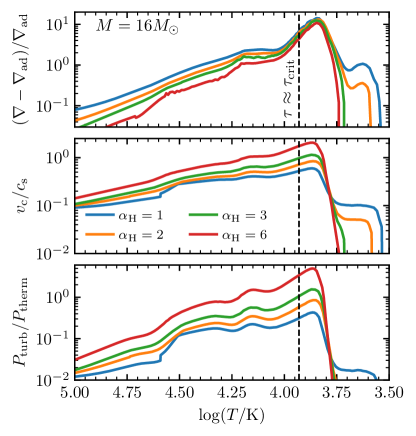
Figure 4: The superadiabaticity (upper panel), convective Mach number (middle panel), and estimated turbulent pressure (lower panel) versus log($T/$K) for $M=16M_{\odot}$, $Z=0.02$ RSG models as $\alpha_{\mathrm{H}}$ varies. The vertical dashed lines indicate where $\tau\approx\tau_{\mathrm{crit}}$ in these models.

In the plane parallel limit, the turbulent pressure term needed to incorporate the effects of the 3D Reynolds stress in a radial 1D model is $P_{\mathrm{turb}}=\rho v_{r}v_{r}\approx\beta\rho v_{c}^{2}$ up to a prefactor $\beta$ typically assumed to be unity (Henyey et al., 1965). This quantity is shown in the lower panel of Fig. 4 for $v_{c}$ given by MESA assuming $\beta=1$. Moving towards the stellar surface, the expected turbulent pressure rises, even exceeding the thermal pressure ($P_{\mathrm{therm}}=P_{\mathrm{gas}}+P_{\mathrm{rad}}$) in the cooler ($T\mathrel{\vbox{ \offinterlineskip\halign{\hfil$#$\cr<\cr\kern 2.0pt\cr\sim\cr\kern-2.0pt\cr}}}10^{4}$ K) regions of the $\alpha_{\mathrm{H}}\geq 3$ models. Due to the intrinsically 3D nature of large-scale convection and the resulting turbulent pressure, the handling of this large expected pressure contribution is another way in which 3D results can guide 1D models.

Moreover, the envelopes of these models are only very loosely gravitationally bound. The lower panel of Fig. 5 shows the local total energy (dashed lines) and cumulative total energy integrated from the surface inwards (solid lines). The upper panel shows the ratio of the cumulative total energy to the gravitational energy. The kinetic energy assuming $v=v_{c}$ is neglected, as it only contributes only a few times $10^{45}$ erg in total for these models. As seen in the upper panel, the gravitational energy and the internal energy nearly cancel, and for our $\alpha_{\mathrm{H}}=1$ model the internal energy exceeds the gravitational binding energy inside the envelope. This demonstrates the precariousness of these RSG envelopes, and why they can become unbound even from small energy deposited there from direct collapse of the He core to a black hole (e.g. Nadezhin 1980; Coughlin et al. 2018). This also highlights the importance of incorporating the envelope’s self-gravity in our 3D calculations.

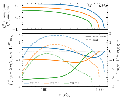
Figure 5: Upper panel: The ratio of the cumulative internal energy to the magnitude of the cumulative potential energy, integrated from the surface. Lower panel: Specific (solid) and cumulative (dashed) total energy (IE + PE) calculated from the surface inward in the envelope of 16 $M_{\odot}$ RSG models with $\alpha_{\mathrm{H}}$=1, 2, 3.

3 3D Model Setup and Equilibration

Name	$R_{\mathrm{IB}}/R_{\odot}$	$R_{\mathrm{out}}/R_{\odot}$	heat source	resolution ($r\times\theta\times\phi$)	duration	$m_{\mathrm{c}}/M_{\odot}$	$M_{\mathrm{final}}/M_{\odot}$
RSG1L4.5	400	22400	“hot plate”	$384\times 128\times 256$	5865 d	12.8	$16.4$
RSG2L4.9	300	6700	fixed $L$	$256\times 128\times 256$	5766 d	$10.79$	$12.9$

Table 1: Simulation properties, including inner boundary ($R_{\mathrm{IB}}$), outer boundary ($R_{\mathrm{IB}}$), heat source (as described in the text), resolution, run duration, core mass $m_{\mathrm{c}}$, and total mass at the simulation end ($M_{\mathrm{final}}$). All models have $\theta=\pi/4-3\pi/4$ and $\phi=0-\pi$, with $\delta r/r\approx 0.01$, and we restrict our analysis to material outside 450$R_{\odot}$. The naming scheme indicates $\log(L/L_{\odot})$.

3.1 Model Setup in Athena++

To explore the 3D convective properties of RSGs, we constructed two large-scale simulations using Athena++. For these simulations, we use spherical polar coordinates with 128 uniform bins in polar angle $\theta$ from $\pi/4-3\pi/4$ and 256 bins in azimuth $\phi$ from $0-\pi$ with periodic boundary conditions in $\theta$ and $\phi$, covering 70.6% of the face-on hemisphere (i.e. solid angle $\Omega=1.41\pi$). Outside of the simulation domain, Athena++ uses ghost zones to enforce its boundary conditions (see Stone et al. 2020 for more details). For the “periodic” boundary in $\theta$, the ghost zones from $\pi/4$ ($3\pi/4$) are copied from last active zones around the $3\pi/4$ ($\pi/4$) boundary, so that the mass and energy flux across the theta boundary is conserved. Although the spherical polar grid in Athena++ can in principle include the whole sphere, such a setup will cause a timestep that is too small to perform these simulations. That is why we only cover the polar region between $\pi/4$ and $3\pi/4$, which is designed to represent a large typical wedge of the star. There are 2 options for a boundary condition in order to conserve mass and energy in the $\theta/\phi$ direction. The method described here is preferred over a reflective boundary condition, which will lead to “splashback” (as is seen at the inner boundary). Athena++ solves the ideal hydrodynamic equations coupled with the time-dependent, frequency-integrated radiation transport equation for specific intensities over discrete angles (Jiang et al., 2014; Jiang, 2021). We adopt the spherical polar angular system as defined in Section 3.2.4 of Jiang (2021) with 120 total angles per grid for the specific intensities. In this initial work, we consider a non-rotating stellar model and neglect magnetic fields. This is likely a safe assumption, as the envelope rotation reduces dramatically as the stars ascend the Hayashi track after core H depletion, though some RSG envelopes may have non-negligible rotation due to interaction or a merger with a companion (see, e.g., Joyce et al. 2020).

The RHD equations are (Jiang, 2021):

$$\begin{split}\frac{\partial\rho}{\partial t}+{\mbox{\boldmath$\nabla$}}\cdot(\rho{\mbox{\boldmath$v$}})&=0,\\ \frac{\partial(\rho{\mbox{\boldmath$v$}})}{\partial t}+{\mbox{\boldmath$\nabla$}}\cdot({\rho{\mbox{\boldmath$v$}}{\mbox{\boldmath$v$}}+{{\sf P_{\mathrm{gas}}}}})&=-\mathbf{G}_{r}-\rho{\mbox{\boldmath$\nabla$}}\Phi,\\ \frac{\partial{E}}{\partial t}+{\mbox{\boldmath$\nabla$}}\cdot\left[(E+P_{\mathrm{gas}}){\mbox{\boldmath$v$}}\right]&=-cG^{0}_{r}-\rho{\mbox{\boldmath$v$}}\cdot{\mbox{\boldmath$\nabla$}}\Phi,\\ \frac{\partial I}{\partial t}+c{\mbox{\boldmath$n$}}\cdot{\mbox{\boldmath$\nabla$}}I&=S(I,{\mbox{\boldmath$n$}}),\end{split}$$ (4)

where $\rho$ is the gas density and $v$ is the flow velocity. The gas pressure tensor and scalar are given by ${\sf P_{\mathrm{gas}}}$ and $P_{\mathrm{gas}}$, respectively. The total gas energy density is $E=E_{g}+\rho v^{2}/2$, where $E_{g}=3P_{\mathrm{gas}}/2$ is the gas internal energy density. Source terms $G^{0}_{r}$ and $\mathbf{G}_{r}$ are the time-like and space-like components of the radiation four-force Mihalas & Mihalas (1984). The frequency-integrated intensity $I$ is a function of time, spatial coordinate, and photon propagation direction $n$.

The mass in the simulation domain is not negligible, and because the envelope is expected to be only loosely bound, it is important to include an accurate gravitational acceleration, which we take to be spherically symmetric, with $-\nabla\Phi=-Gm(r)/r^{2}$. Here $G$ is the gravitational constant, $r$ is the radial coordinate, and $m(r)$ is the total mass inside $r$. We calculate $m(r)$ as the sum of the “core” mass interior to the inner boundary (IB) and the total mass between the IB and $r$ at each time step. The gas temperature is $T=(P_{\mathrm{gas}}\mu m_{\mathrm{p}})/(k_{\mathrm{B}}\rho)$, where $k_{B}$ is the Boltzmann constant, and $m_{p}$ is the proton mass, with mean molecular weight $\mu=0.643$ to match our MESA models. A radiation temperature $T_{r}$ can be calculated from the radiation energy density $E_{r}$ included in the $G^{0}_{r}$ source term as $T_{r}=(E_{r}/a_{r})^{1/4}$ where $a_{r}=4\sigma_{\mathrm{SB}}/c$ is the radiation constant and $\sigma_{\mathrm{SB}}$ is the Stefan-Boltzmann constant; this is typically, but not necessarily, identical to $T$.

To calculate the radiation energy and momentum source terms, the lab frame intensity $I({\mbox{\boldmath$n$}})$ with angle $n$ is first transformed to the co-moving frame intensity $I_{0}({\mbox{\boldmath$n$}}_{0})$ with angle ${\mbox{\boldmath$n$}}_{0}$ via Lorentz transformation (Mihalas & Mihalas, 1984; Jiang, 2021). The source terms describing the interactions between gas and radiation in the comoving frame are

$$S_{0}(I_{0},{\mbox{\boldmath$n$}}_{0})=c\rho\kappa_{aP}\left(\frac{ca_{r}T^{4}}{4\pi}-J_{0}\right)+c\rho(\kappa_{s}+\kappa_{aR})\left(J_{0}-I_{0}\right),$$ (5)

where $\kappa_{aR}$ and $\kappa_{aP}$ are the Rosseland and Planck mean absorption opacities determined by interpolation of the OPAL opacity tables (Iglesias & Rogers, 1996), and $\kappa_{s}$ is the electron scattering opacity, all evaluated in the comoving frame. The angular quadrature of the intensity in the co-moving frame is $J_{0}=\int I_{0}({\mbox{\boldmath$n$}}_{0})d\Omega_{0}/(4\pi)$. After the specific intensities $I_{0}({\mbox{\boldmath$n$}}_{0})$ are updated in the co-moving frame, they are Lorentz transformed back to the lab frame. The radiation momentum and energy source terms $G^{0}_{r}$ and $\mathbf{G}_{r}$ are calculated by the differences between the angular quadratures of $I({\mbox{\boldmath$n$}})$ in the lab frame before and after adding the source terms. See Jiang (2021) for more details of the implementation. The hydrodynamic equations are solved using the standard Godunov method in Athena++ (Stone et al., 2020). Similar numerical methods and setup have been successfully used to model stellar envelopes in different locations of the HR diagram (Jiang et al., 2015, 2018).

3.2 RSG Setup and Model Evolution

We used the NASA supercomputer Pleiades to run two 3D RHD simulations. Each run takes about two months to finish with 80 skylake nodes in Pleiades. For this study, we motivate our initial and boundary conditions with the fiducial $15.4M_{\odot}$, $Z=0.02$, $\alpha_{\mathrm{H}}=3$ model at the end of core C burning discussed in §2 (shown in green in the left panels of Fig. 2). Our first model, referred to hereafter RSG1L4.5, is initialized in 3D by assuming a purely radiative envelope with luminosity equal to the radiative luminosity at $r=400R_{\odot}$ in the MESA model (which is a few % of the total luminosity). The mass and radius of the IB are $400R_{\odot}$ and 12.8$M_{\odot}$. To generate the initial conditions, the temperature ($T=7.19\times 10^{4}$ K) at the IB is first set to equal the $400R_{\odot}$ coordinate in the MESA model, and density ($\rho=5.45\times 10^{-8}$ g/ cm^-3) selected to approximately recover the $15.4M_{\odot}$ total mass. To perturb from the radiatively stable initial conditions and supply the convective luminosity, we increase the temperature at the IB by $10\%$ compared with the initial condition (a “hot plate”), while density is fixed and velocity is reflective at the inner boundary, akin to the setup of Jiang et al. (2018). This boundary condition produces a radiative layer near the bottom with the desired luminosity, which causes the envelope away from the bottom boundary to be convective. In this setup, we do not know in advance what the luminosity will be. RSG1L4.5 was one of 3 initial runs with this inner boundary condition; the other two at 20% and 40% Temperature increases gained mass too rapidly and never reached a convective steady state.

All our analysis will be done in the convective region starting from $\approx$ 450$R_{\odot}$. As convection sets in, the luminosity reaches $\log(L/L_{\odot})=4.5$, with some periodic and stochastic variability which we will discuss in more detail in §4.4. Because mass flux through the inner boundary cannot be exactly 0 on a spherical polar mesh even with our reflective velocity boundary condition, a small amount of additional mass enters the simulation domain as time goes on. At the end of the simulation, the total mass of this model is 16.4$M_{\odot}$. This 6.5% increase in the total mass of the star ($\approx$20% in the mass inside our simulation domain) is not of concern, as the aim of this work is to create realistic 3D envelope models to study the convective structure, not to diagnose a mass-luminosity relation in 3D models (which would also be sensitive to core properties). The simulation domain for this model is 384 radial zones, with $\delta r/r\approx 0.01$, with a free outer boundary at $r=22400R_{\odot}$. The choice of a large simulation domain was motivated, in part, to capture any wind structure or extended atmosphere, make sure we capture the stellar photosphere so that the outer boundary is always in the optically thin limit for the radiation field, as well as to provide ample space for expansion in explosions of this envelope model in forthcoming work. With a logarithmic radial grid spacing, the large outer boundary is achieved with small additional cost for our simulation, and $87$ zones lie within $r<1000R_{\odot}$.

Our second model, referred to hereafter RSG2L4.9, is initialized with the same method as RSG1L4.5 for the region that will become convective. This model has the IB at 300$R_{\odot}$ with 10.79$M_{\odot}$ enclosed, and the total initial mass at 14$M_{\odot}$. The simulation domain has 256 radial zones (98 at $r<1000R_{\odot}$) with $\delta r/r\approx 0.01$, with a free outer boundary at $r=6700R_{\odot}$, still far away from the stellar surface. Between $300R_{\odot}$ and $400R_{\odot}$, the initial profile is constructed with the radiative luminosity to be $10^{5}L_{\odot}$ and this is kept fixed in the inner boundary (“fixed $L$”). This serves the same purpose as the boundary condition used in the previous model to drive convection for the region above. We therefore similarly only perform our analysis for the region above $\approx$450$R_{\odot}$. We first run for 740 days with fixed total $F_{r}$ at the inner boundary (including advection and diffusion). After an initial relaxation period, this scheme begins to add mass somewhat rapidly, so we switch to fixing only the diffusive $F_{\mathrm{rad,0}}$ at the inner boundary. This leads to a small, steady decrease in the total envelope mass from the inner boundary. At the end of the simulation, the total mass of this model is 12.9$M_{\odot}$. In both cases, most of the mass change happens during the initial transient relaxation from the initial conditions to a convective structure. From day 4500 to the end of the simulation, the mass inside the simulation domain changes by less than 1% ($0.03M_{\odot}$) for RSG1L4.5, and 10% ($0.2M_{\odot}$) for RSG2L4.9. The properties of these models are summarized in Table 1.

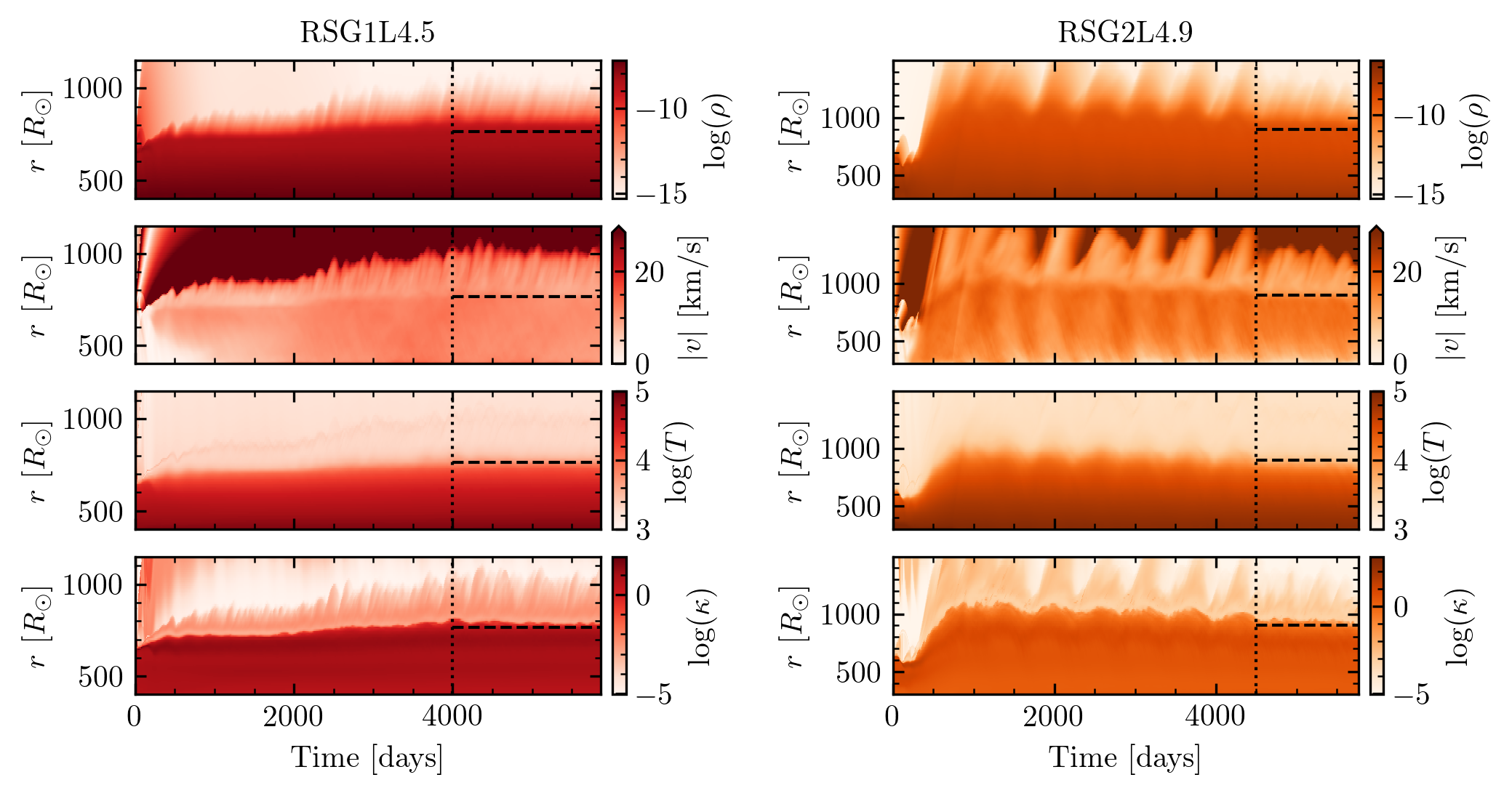
Figure 6: History of the averaged radial profiles for our RSG1L4.5 (red, left) and RSG2L4.9 (orange, right) models. Top to bottom show log(density), convective velocity, log(temperature), and log(opacity). All logarithms are base 10 and units inside the logarithms are cgs, and velocites are reported in km/s. Vertical dotted lines indicate when the envelope appears to have reached a convective steady state. Horizontal dashed lines approximate the region where some fraction of the stellar area has $\tau>\tau_{\mathrm{crit}}$.

Radial profiles of both simulations as a function of time are shown as space-time diagrams in Fig. 6. Radial density, opacity, and temperature are calculated by finding the volume-weighted average over spherical shells at each time (which we hereafter denote with $\langle\cdots\rangle$), and the magnitude of the velocity, is calculated from the mass-weighted average over spherical shells (which we hereafter denote with $\langle\cdots\rangle_{m}$), $|v|=\sqrt{\langle v_{r}^{2}+v_{\theta}^{2}+v_{\phi}^{2}\rangle_{m}}$. Horizontal dashed lines approximate the location where radiation begins to dominate the energy transport at late times. Inside the dashed line, convection is expected to resemble MLT, with denser material sinking as less dense material rises. We will explore this expectation in more detail in §4.4 and 5. For computational reasons, both models have density floors imposed with $\rho_{\mathrm{floor}}=5.35\times 10^{-16}$ g/cm³. The fast-moving low-density material at very large radii is caused by negligible amounts of density-floor material falling onto the star due to gravity.

The two simulations begin with an initial transient phase, as convection sets in from the unstable spherically symmetric initial conditions. In RSG1L4.5, the intial transient phase is accompanied by some material being launched outwards, falling back onto the stellar surface around day 2500. Additionally, convection begins to appear at the density inversion near the stellar surface, and makes its way to the IB by $\approx 1000$ days. By day 2000, the amplitudes of the convective velocities steady and by day 4000 the RSG1L4.5 simulation appears to have fully settled into equilibrium, with regular fluctuations in the stellar properties particularly in the region above $\tau=\tau_{\mathrm{crit}}$.

In RSG2L4.9, the fixed luminosity at the IB triggers convection at small radii in addition to the surface, so convection sets in quickly. The initial transient causes a sharp increase in the mass contained in the stellar envelope coming from the inner boundary, accompanied by a rapid expansion of the envelope around day 500. With the change in inner boundary condition at day 740, the rapid growth ceases, and by day 2000 the model begins to settle into a pattern of semi-regular oscillations. By day 4500, the amplitude of radial fluctuations dies down and the envelope exhibits similar steady-state behavior to the RSG1L4.5 simulation with larger radial extent and higher velocities. We now check this apparent steady-state behavior for both simulations.

3.3 Defining a ‘Steady State’

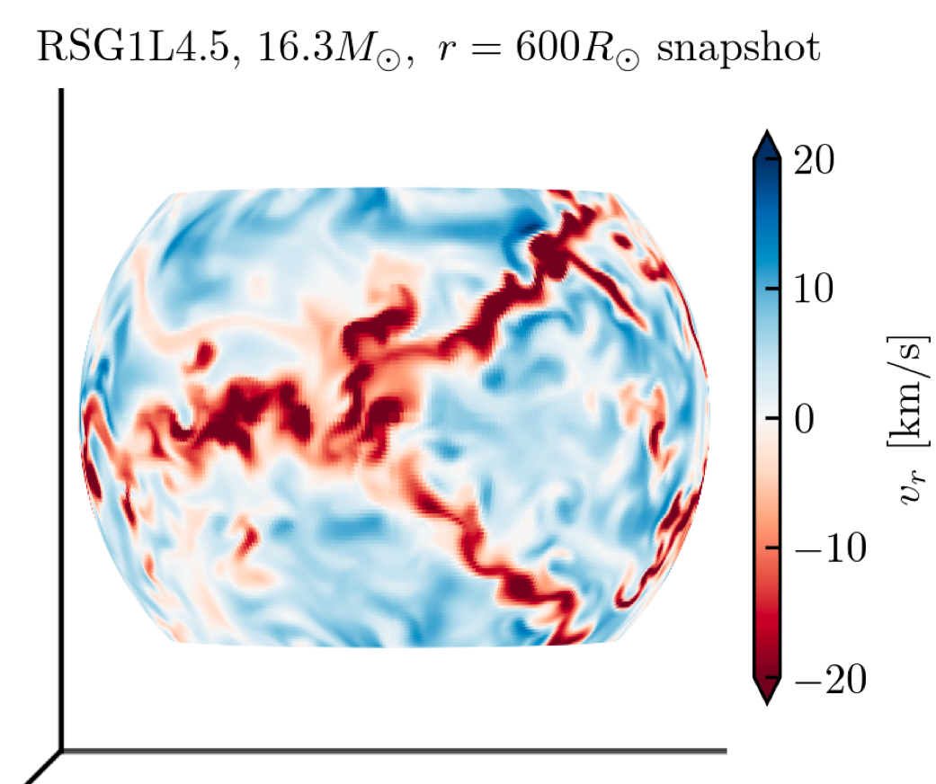
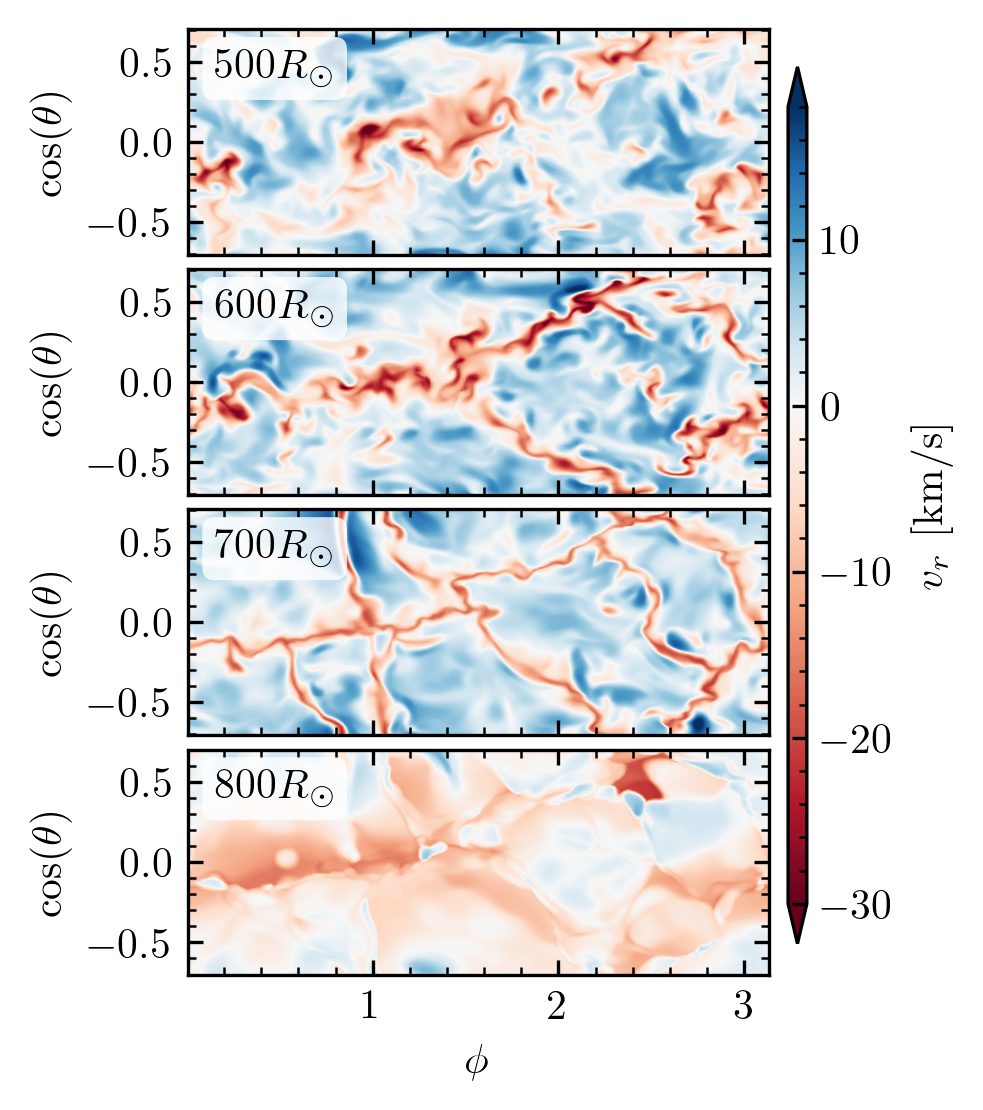
Figure 7: Left: Surface rendering of the radial velocity fluctuations at $r=600R_{\odot}$ in RSG1L4.5 at day 4707. Right: Snapshot of radial velocity slices for the same model. Panels show radial slices at $r=500R_{\odot}$ (top) to $800R_{\odot}$ (bottom) in $100R_{\odot}$ intervals, and axes show the extent in azimuth $\phi$ and co-polar angle cos($\theta$). The volume-weighted mean sound speed is 33 km/s at $r=500R_{\odot}$, 26 km/s at $600R_{\odot}$, 19 km/s at $700R_{\odot}$, and 8 km/s at $800R_{\odot}$.

By the end of the simulations, both models have thermal and kinetic energy content $E_{\mathrm{fluid}}=\int(E+E_{r})\mathrm{d}V$ comparable to the binding energy $E_{\mathrm{bind}}=\int(\rho\Phi)\mathrm{d}V$, with a ratio of $E_{\mathrm{fluid}}/|E_{\mathrm{bind}}|$ of 0.23 for RSG1L4.5 (with $E_{\mathrm{tot}}=E_{\mathrm{fluid}}+E_{\mathrm{bind}}=-3.0\times 10^{47}$erg extending the volume to $\Omega=4\pi$) and 0.32 for RSG2L4.9 ($E_{\mathrm{tot}}=-1.4\times 10^{47}$erg). The comparable gas and binding energies reinforce our choice of including the envelope mass in our gravitational.

The convective plumes show large ($\mathrel{\vbox{ \offinterlineskip\halign{\hfil$#$\cr>\cr\kern 2.0pt\cr\sim\cr\kern-2.0pt\cr}}}200R_{\odot}$) vertical and lateral extents, leading to a nearly-radius-independent velocity profile with an-order-of-magnitude scatter, shown in Fig. 7. When fluid flow is this coherent, the velocity field will be time-correlated for around an eddy-turnover time at any given spatial location. Beyond this timescale, we expect no memory of past convective plumes at a fixed coordinate. To start our exploration of the timescale required for the model to reach equilibrium, we calculate the autocorrelation of the radial velocity at fixed coordinates. The autocorrelation function for an arbitrary time-dependent parameter $Y(t)$ is defined for time lag $\Delta t$ by

$$\mathrm{acf}(Y,\Delta t)=\frac{\int{(Y(t)-\bar{Y})(Y(t+\Delta t)-\bar{Y})\mathrm{d}t}}{\int(Y(t)-\bar{Y})^{2}\mathrm{d}t},$$ (6)

where $\bar{Y}$ is the time-averaged value. Fig. 8 shows the autocorrelation function for the radial velocity, acf($v_{r},\Delta t$), for a few different radii in each model. Dark lines give the mean of the autocorrelation functions at 169 angles distributed across the stellar model, and the shaded areas give the standard deviation of the acf at each radius. Only radial velocities after day 1000 are considered for each model. The less luminous RSG1L4.5 model stays correlated for $\approx$550 days, whereas the more luminous RSG2L4.9 model decorrelates faster, over a timescale of $\approx$300 days. This is because the more luminous model exhibits larger convective velocities as required to carry the flux, even though the mass and radii are comparable. These timescales are short compared to the simulation duration, so we can proceed in our analysis with additional confidence that both models have reached their convective steady state after $\approx$4000 days.

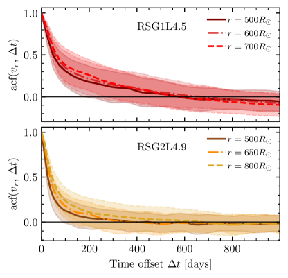
Figure 8: Average autocorrelation of radial velocities across different angles at different radii for the RSG1L4.5 model (upper panel) and the RSG2L4.9 model (lower panel) as a function of the time lag. All data in this plot are after the simulations have run for 1000 days. The shaded region gives the standard deviation of the acf across the different angles.

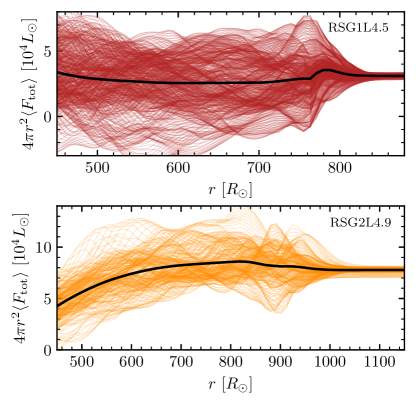
Figure 9: Volume-average of $4\pi r^{2}((E+P_{\mathrm{gas}})v_{r}+F_{\mathrm{r},\hat{r}}-(\rho v_{r}\Phi))$ at different times (thin colored lines) compared to the time-average (solid black line) for our RSG1L4.5 (red, upper panel) and RSG2L4.9 (orange, lower panel) models outside $r=450R_{\odot}$.

A direct check as to whether the models have reached a convective steady state is to explore the RHD equations for the time-averaged profiles. The momentum equation quickly equilibrates such that $\partial\rho{\mbox{\boldmath$v$}}/\partial t\rightarrow 0$ when taking the time-average on a dynamical timescale (i.e. the sound-crossing time across a pressure scale height, 10s to 100s of days in the outer envelope), but the energy equation will only reach equilibrium in our region of interest as convection is able to distribute the luminosity over a few eddy turnover times, which is significantly longer. Combining and rearranging RHD Eqs. (4) including the source term

$$G^{0}_{r}=\frac{\partial E_{\mathrm{r}}}{\partial t}+\nabla\cdot\boldsymbol{F}_{\mathrm{r}},$$ (7)

where ${\mbox{\boldmath$v$}}{F}_{r}$ is the total radiation flux (including radiative diffusion $F_{\mathrm{rad,0}}=-1/3(c/\kappa\rho)(\mathrm{d}a_{r}T_{r}^{4}/\mathrm{d}r)$ and advection $F_{\mathrm{adv}}=E_{r}v_{r}$), with $g=-\nabla\Phi\cdot\hat{r}$, for spherically symmetric $\Phi(r)$, we recover

$$\frac{\partial}{\partial t}(E+E_{\mathrm{r}})+\nabla\cdot[(E+P_{\mathrm{gas}})\boldsymbol{v}+\boldsymbol{F}_{\mathrm{r}}-(\rho\boldsymbol{v}\Phi)]$$ (8)

$$=-\Phi\nabla\cdot(\rho\boldsymbol{v})=-\Phi\frac{\partial}{\partial t}\rho.$$

In a steady state, $\partial/\partial t\rightarrow 0$ when we take the time average $\langle\cdots\rangle_{t}$. Taking the radial component of the divergence we find

$$\left\langle\frac{1}{r^{2}}\frac{\partial}{\partial r}[r^{2}(E+P_{\mathrm{gas}})v_{r}+r^{2}F_{\mathrm{r},\hat{r}}-r^{2}(\rho v_{r}\Phi)]\right\rangle_{t} =0.$$ (9)

Thus if $r^{2}\left\langle(E+P_{\mathrm{gas}})v_{r}+F_{\mathrm{r},\hat{r}}-(\rho v_{r}\Phi)\right\rangle_{t}\equiv r^{2}\langle F_{\mathrm{tot}}\rangle$ is spatially constant, the model can be considered to have equilibrated. This expression is equivalent to the time-average of the volume-weighted average of the total luminosity $L_{\mathrm{tot}}$, including enthalpy, gravity, kinetic energy, and radiation terms, divided by 4$\pi$. Though there is a net change in $L_{\mathrm{tot}}$ due to mass gained/lost near the IB, in the region of interest, our steady state criteria are sufficiently satisfied by both models in the region of interest, as shown in Fig. 9. The transparent colored lines show the volume-averaged total luminosity from days 4001$-$5864 in approximately 3 day intervals for the RSG1L4.5 model (red) and evolution from day 4501$-$5766 in approximately 5 day intervals for the RSG2L4.9 model (orange). The solid black lines give the time-average of this quantity, whose variance at different radii is significantly less than the scatter at different times. The small number of distinct convective plumes implies a fundamental variance in the stellar luminosity reflected in the scatter at large radii that we discuss in more detail in §4.4.

4 3D Model Properties

Having shown how to initiatlize a 3D RSG model and evolve it to its effectively equilibrium state, we now will describe the properties of the resulting models, compare to prior work, and discuss some of the unique properties of these highly luminous models.

4.1 Convective Properties and Comparison to Prior 3D CO${}^{\texttt{5}}$BOLD RSG Work

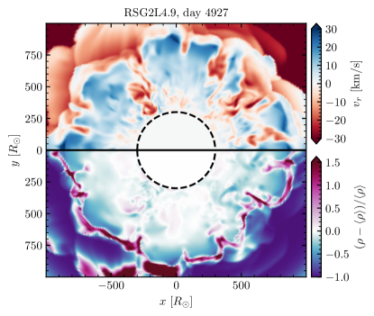
Figure 10: Equatorial ($\theta=\pi/2,z=0$) slice of a characteristic snapshot of the RSG2L4.9 model, showing (upper half of the figure:) radial velocities and (lower half of the figure:) density fluctuations relative to the shellular volume-averaged density at each radius. The simulation domain is from $\phi=0$ to $\pi$; thus the image is reflected about $y=0$ as indicated by the axis labels.

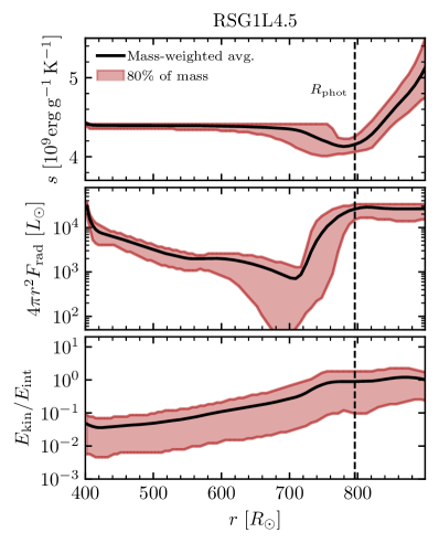
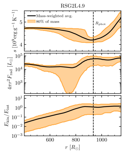
Figure 11: Specific entropy (top panels), radiative luminosity (middle panels), and ratio of the turbulent kinetic energy to the internal energy (bottom panels) in our RSG1L4.5 model at day 4707 (red, left) and RSG2L4.9 at day 4927 (orange, right). Mass-weighted averages are shown in black, with 80% of the mass lying within the shaded regions. The 1D photosphere, where $\langle{L(r)}\rangle=4\pi r^{2}\sigma_{\mathrm{SB}}\langle{T_{r}(r)}\rangle^{4}$, is given by the vertical dashed line.

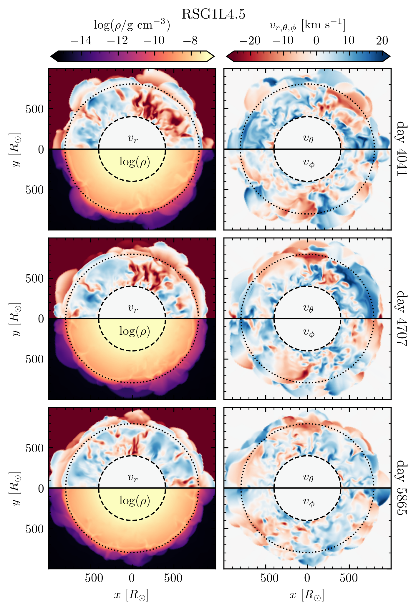
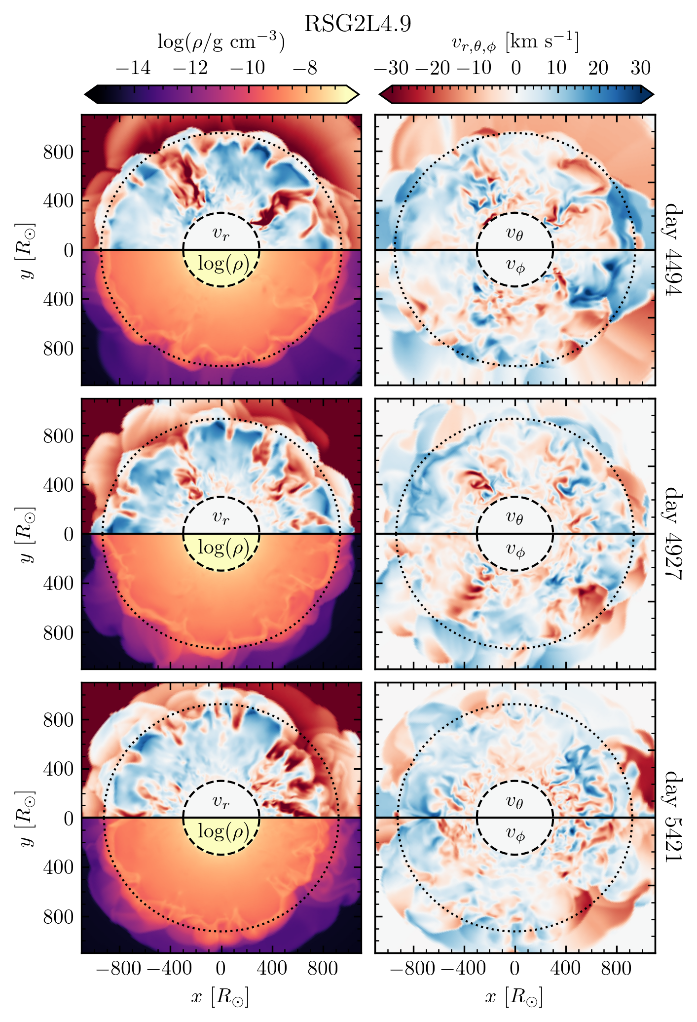
Figure 12: Equatorial ($\theta=\pi/2,z=0$) slices for our RSG1L4.5 (left 6 panels) and RSG2L4.9 (right 6 panels) models at different simulation times. At each time for each model, the left panel shows radial velocity (red/blue colors) and density (orange/purple colors) is beneath. The right panel shows polar tangential velocity ($v_{\theta}$) and azimuthal velocity ($v_{\phi}$) is beneath. The simulation domain is from $\phi=0$ to $\pi$; thus the y-axis is reflected in the lower half of each panel as indicated by axis labels. With $\theta=0$ along the $+z$ axis and $\phi=0$ along the $+x$ axis, $v_{\theta}>0$ indicates material flowing into the page, and $v_{\phi}>0$ indicates material flowing clockwise around the page (due to the inverted y-axis). The dashed line indicates the simulation inner boundary and the dotted line denotes the 1D photosphere.

Aspects of the observable 3D structure of RSGs have been studied in a series of pioneering papers (e.g. Chiavassa et al. (2009, 2010b, 2011b, 2011a); Kravchenko et al. (2018)) using the RHD “star-in-a-box” COnservative COde for the COmputation of COmpressible COnvection in a BOx of L Dimensions, L=2,3 (CO${}^{\texttt{5}}$BOLD, Freytag et al., 2002, 2010, 2012). In those simulations, the computational grid was cubic equidistant with typical mesh spacing of $\approx 8.6R_{\odot}$, with LTE radiation transport by short characteristics using opacity tables as function of $P,\ T$ interpolated from PHOENIX data at $T\mathrel{\vbox{ \offinterlineskip\halign{\hfil$#$\cr<\cr\kern 2.0pt\cr\sim\cr\kern-2.0pt\cr}}}12,000\,$K (Hauschildt et al., 1997) and OPAL values (Iglesias et al., 1992) at higher $T$. The EOS included ideal gas and ionization, but radiation was only present in the energy equation, and not as a pressure source. The gravitational potential was modeled by a Plummer potential $\Phi=-GM_{*}/(r_{0}^{4}+r^{4}/\sqrt{1+(r/r_{1})^{8}})^{1/4}$ fixed to the static Cartesian mesh with $M_{*}=12M_{\odot}$ and $3M_{\odot}$ of material contained in the simulation domain, and the luminosity was supplied via an energy source within the inner Plummer radius ($r_{0}$).

That work focused on stellar properties at low optical depth, where radiation transport dominates, and have been compared to recent tomagraphic observations of nearby RSGs to interpret their surface convective structure (e.g., Kravchenko et al., 2019, 2020, 2021). The neglect of radiation pressure deep within the star inhibited the ability to correctly simulate the deeper nearly-constant-entropy convective zone there. Hence, the convective flux in the interior of those RSG models is significantly lower than the radiative flux, with radiation carrying over 80% of the flux everywhere. Because of this, those simulations exhibit a positive entropy gradient out to $\approx$75% of the stellar radius (see Fig. 3 of Chiavassa et al. 2011a). While this is no concern when restricting analysis to the turbulent surface layers where the entropy profile does decline, it is counter to the theoretical expectations for a fully turbulent RSG envelope, which should have a nearly-flat, declining entropy profile throughout the convective envelope, with enthalpy and kinetic flux accounting for a significant fraction of the total flux.

In agreement with the CO${}^{\texttt{5}}$BOLD models, our Athena++ RSG simulations show a handful of large-scale, coherent convective plumes across the star, with radial velocities of tens of km/s and density fluctuations of 10% increasing to factors of a few at larger radii (see Figs. 7 and 10). As emphasized by Stein & Nordlund (1998), we see a topology of large area upwellings surrounded by narrow lanes of downward flows. Additionally, the specific entropy, radiative luminosity, and ratio of kinetic to thermal energy density in representative snapshots of our two models are shown in Fig. 11. The red/orange shaded regions give a sense of the scatter. Like in the CO${}^{\texttt{5}}$BOLD models, we observe a ‘halo’ of bound, high-entropy material above the conventional photosphere, with density fluctuations exceeding an order of magnitude in the outer-most parts of the star. The entropy profile in the interior of our Athena++ models is nearly adiabatic, declining slightly out to $100-200R_{\odot}$ beneath the 1D photosphere, and declining more rapidly as radiation is able to carry more of the flux. These entropy profiles are similar to those seen in lower-luminosity RHD models (e.g. Stein & Nordlund, 1998; Magic et al., 2015).

Following Chiavassa et al. (2011a), we define the 1D photosphere by calculating 1D radial profiles of the luminosity $\langle L(r)\rangle$ and radiation temperature $\langle T_{r}(r)\rangle$; $r=R_{\mathrm{phot}}$ is then defined as the location where $\langle L(r)\rangle=4\pi r^{2}\sigma_{\mathrm{SB}}\langle T_{r}(r)\rangle^{4}$. The energy transport in the stellar interior is dominated by convection, and radiation carries $\approx 10\%$ of the luminosity in the convective region. Moreover, the turbulent kinetic energy density from the vigorous convective motions dominates over the thermal energy in the outer envelope, in agreement with the findings of (Chiavassa et al., 2011a).

4.2 Stochastic Angular Momentum

The 3D properties of convection in RSG interiors are also of interest for predicting properties of the remnant in failed SNe (e.g. Coughlin et al., 2018; Quataert et al., 2019). Recently, Antoni & Quataert (2021) completed a detailed study of convective fluid motion with applications to collapsing RSGs using 3D hydrodynamical simulations of idealized RSG models spanning a factor of 20 in stellar radius. Their work considers an ideal gas with polytropic index $\gamma=1.462$ in a Plummer potential $\Phi=-GM/(r^{n}+a^{n})^{1/n}$ with $n=8$ for a smoothing radius $a\ll r_{o}$ in their dimensionless code units where $r_{o}=R_{\mathrm{phot}}/6$. This converges to a point mass in their region of interest. These pure-hydro simulations enforce a photospheric radius by providing a cooling sink at large fixed radii and smoothly decreasing the temperature outside the photosphere to be equal to their temperature floor. Their study focused on quantifying the randomly distributed angular momentum of the inner layers of the convective RSG envelope, and how these shells evolve during later collapse.

In our models, we likewise observe large tangential velocity fluctuations due to the random convective fluid motion with coherence across many scale heights. Fig. 12 shows the radial and tangential components of the fluid velocity for equatorial ($z=0$, $\theta=\pi/2$) slices through our Athena++ models, as well as the density structure. The large radial velocity plumes carry material out beyond $R_{\mathrm{phot}}$ (the dotted lines). As the fluid becomes optically thin, the temperature plummets and the pressure scale height drops, and the very large convective plumes fragment into smaller bubbles of surface convection. This is especially apparent in the more luminous RSG2L4.9 model (right 6 panels). Additionally, there is some outward-moving high-density material evident at large radii. We will discuss this material in greater detail in §4.4. The velocities in $r,\ \theta,$ and $\phi$ are comparable, with values of tens of km/s. The tangential flows ($v_{\theta}$ and $v_{\phi}$) exhibit smaller-scale structures at smaller radii, in agreement with the results of Antoni & Quataert (2021).

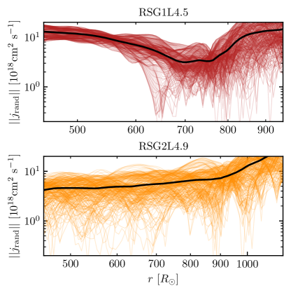
Figure 13: Specific angular momentum profiles at different snapshots (thin colored lines), compared to the time-average (solid black lines), for our RSG1L4.5 (red, upper panel) and RSG2L4.9 models (orange, lower panel).

Although the net angular momentum in the envelope is nearly zero, these tangential velocity fluctuations result in finite specific angular momentum $j_{\mathrm{rand}}$ at a given radius at any given time. The magnitude (denoted $||\cdots||$) of the mass-weighted average of the random specific angular momentum profiles, equivalent to $||j_{\mathrm{rand}}||=||\langle\rho{\mbox{\boldmath$v$}}\times{\mbox{\boldmath$r$}}\rangle/\langle\rho\rangle||$, is shown in Fig. 13. As in Fig. 9, faint colored lines correspond to individual snapshots in our models, and the solid black line indicates the time-average. In agreement with Antoni & Quataert (2021), these simulations exhibit relatively flat specific angular momentum profiles, pointing to the non-local coherent nature of the convective plumes. Due to the high $\sim 10$ km/s tangential velocities and the fact that our simulation domain emphasizes large radii ($r>400R_{\odot}$), we find specific angular momenta of $10^{18}-2\times 10^{19}$cm²/s throughout our simulation domain. Transforming to a local rotational velocity $\omega_{\mathrm{rot}}=||j_{\mathrm{rand}}||/r^{2}$, this corresponds to a range of $\omega_{\mathrm{rot}}$, declining from $\approx$10^-3 rad/day to 10^-4 rad/day before rising outside $R_{\mathrm{phot}}$ in RSG1L4.5, and a flatter, slightly declining time-averaged profile around a few $\times 10^{-3}$ rad/day in RSG2L4.9 with the scatter between snapshots ranging from a few times $10^{-5}$ to 8$\times 10^{-4}$ rad/day. These values are slightly larger than those reported by Antoni & Quataert (2021), likely owing to the larger convective velocities present in our simulations. Following Quataert et al. (2019), we should reduce our estimate by the expected scaling for the larger number of eddies available in a $4\pi$ steradian simulation, which would then be a factor of $(\Omega/4\pi)^{1/2}\approx 0.6\times$ smaller. This modifies our values to a few$\times 10^{17}-10^{19}$ cm²/s, which are closer to those found by Antoni & Quataert (2021).

4.3 Nature of 3D Convective Structure

In a clumpy or turbulent medium, density fluctuations are often characterized by $\sigma_{\rho}^{2}=\frac{\langle\rho^{2}\rangle}{\langle\rho\rangle^{2}}$ (see, e.g. Owocki & Sundqvist, 2018, in the context of stellar winds). For a log-normal density distribution typical of convective flows, this is related to the characteristic density fluctuations by $(\delta\rho/\rho)^{2}=\sigma_{\ln\rho}^{2}=\ln\left(\frac{\langle\rho^{2}\rangle}{\langle\rho\rangle^{2}}\right)$ (Schultz et al., 2020). Locally, the buoyant acceleration felt by a perturbed fluid element with density $\rho+\delta\rho$ will be related to gravity as $a\approx(\delta\rho/\rho)g$. The perturbation will approximately traverse a scale height (or mixing length) in time $t$ with velocity $v\sim~{}a~{}t\sim(\delta\rho/\rho)(H/v)g$. Thus $v^{2}\sim~{}gH(\delta\rho/\rho)$, or $\delta\rho/\rho\propto\mathcal{M}^{2}$, where $\mathcal{M}=v/c_{\mathrm{s}}$ is the Mach number. Fig. 14 shows the characteristic density fluctuations $\delta\rho/\rho=\sqrt{\sigma^{2}_{\ln\rho}}$ versus the average Mach number in each spherical shell for $450R_{\odot}<r<R_{\mathrm{phot}}$ using the snapshots shown in Fig. 12. The area fraction of the star where the optical depth along a radial line of sight is greater than the angle-averaged $\tau_{\mathrm{crit}}$, $A(\tau>\tau_{\mathrm{crit}})$, is also shown. Where $A(\tau>\tau_{\mathrm{crit}})$ is large, the fluid in both models follows closely with the expected $\delta\rho/\rho\propto\mathcal{M}^{2}$ scaling. As $A(\tau>\tau_{\mathrm{crit}})$ decreases and convection no longer dominates the energy transport everywhere, the scaling flattens and the density fluctuations begin to saturate. Other snapshots exhibit the same behavior in both models.

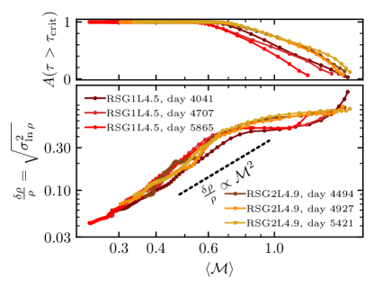
Figure 14: Characteristic density fluctuations versus the (volume-weighted) average turbulent mach number for the 6 model snapshots shown in Fig. 12. Each point corresponds to the averaged value in each radial shell. The upper panel shows the area fraction of the star at each location with $\tau<\tau_{\mathrm{crit}}$ along a radial line of sight. Where $A(\tau>\tau_{\mathrm{crit}})=1$ we expect the flow to follow the $\delta\rho/\rho\propto\mathcal{M}^{2}$ scaling, indicated by the black dashed line.

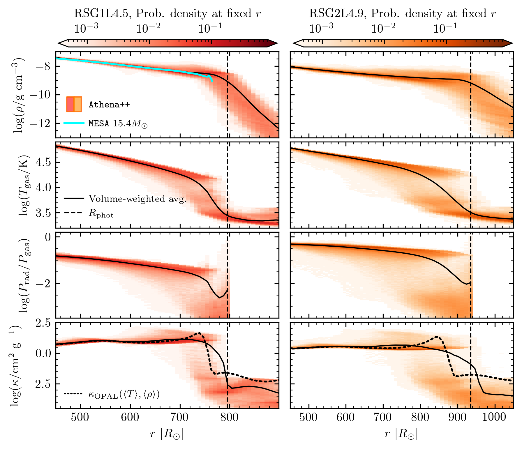
Figure 15: Top to bottom: Density, temperature, $P_{\mathrm{rad}}/P_{\mathrm{gas}}$ ratio, and opacity for our RSG1L4.5 model at day 4707 (red, left panels) and our RSG2L4.9 model at day 4927 (orange, right panels). Color saturation indicates the volume-weighted probability of finding a fluid element at a given ($\rho,T,H/r,P_{\mathrm{rad}}/P_{\mathrm{gas}},\kappa$) at each radial coordinate, and solid black lines give the volume-weighted averages of each (non-log) quantity ($\langle\rho\rangle,\langle T\rangle,\langle H/r\rangle,\langle P_{\mathrm{rad}}/P_{\mathrm{gas}}\rangle,\langle\kappa\rangle$). The vertical black dashed line is $R_{\mathrm{phot}}$. As $P_{\mathrm{rad}}$ is not defined in the free-streaming regime, the ratio $P_{\mathrm{rad}}/P_{\mathrm{gas}}$ is only shown for $r\leq R_{\mathrm{phot}}$. The $\kappa$ panels (bottom) show both the volume-averaged opacity $\log(\langle\kappa\rangle)$ reported by Athena++ (solid lines), and the recovered OPAL opacity (dotted lines) from the volume-averaged $T$ and $\rho$ profiles. For reference, the cyan line in the upper left panel shows the density profile of the fiducial MESA model (green line in the left panels of Fig. 2).

Other stellar properties also exhibit large fluctuations at a given radius, particularly in the outer stellar layers, where the transition to radiation-dominated energy transport does not happen at one single radial location. Fig. 15 shows radial profiles of the density, gas temperature, $P_{\mathrm{rad}}/P_{\mathrm{gas}}$ ratio, and opacity for characteristic snapshots of RSG1L4.5 and RSG2L4.9 (day 4707 and 4927, respectively), with solid black lines showing the volume-averaged radial profiles and color indicating the scatter. The density, which falls like $1/r^{2}$ in the nearly-adiabatic interior, exhibits variations over 2-3 orders of magnitude near $R_{\mathrm{phot}}$, with an extended atmosphere which is absent in 1D models (compare to the cyan line in the upper left panel).

The ratio of radiation to gas pressure is also significant, with $\langle P_{\mathrm{rad}}/P_{\mathrm{gas}}\rangle=0.15$ at $r=450R_{\odot}$ in the RSG1L4.5 model, and $\langle P_{\mathrm{rad}}/P_{\mathrm{gas}}\rangle=0.48$ at $r=450R_{\odot}$ in RSG2L4.9 owing to the larger luminosity and lower density within the envelope. Moreover, rather than a smooth transition from the H opacity peak to electron scattering, the temperature and opacity display bimodal behavior in the $\approx 100-200R_{\odot}$ region beneath $R_{\mathrm{phot}}$. This bimodality is not seen in the $\rho$ profile. Near and even within the 1D photosphere, at some angular locations outer convective plumes exhibit large opacities, whereas other angular locations are dominated by cool material beyond the H opacity peak. Due to the dramatic 4-order-of-magnitude differences in opacity of different material at fixed radius, a linear volume-average of the opacity, given by the black line in the bottom panels, will necessarily favor the high-opacity material. Most notably, the opacity above which $L$ locally exceeds $L_{\mathrm{Edd}}$, $\kappa_{\mathrm{Edd}}=4\pi Gcm/L_{\mathrm{surf}}$, is $\kappa_{\mathrm{Edd}}\approx 6$ cm²/g for RSG1L4.5 and $\kappa_{\mathrm{Edd}}\approx 2$ cm²/g for RSG2L4.9. In the bimodal transitionary region, a large fraction of the material has $\kappa>\kappa_{\mathrm{Edd}}$! Moreover, the presence of bimodal temperature and opacity distributions in this transitionary region causes a smearing out of the H-opacity peak, so the H opacity cliff, predicted by OPAL using the volume-averaged $\rho$ and $T$ profiles, is less steep in the 3D simulation.

This transitionary region corresponds to the place where $A(\tau>\tau_{\mathrm{crit}})$ goes from 1 to 0 and the turbulent motions deviate from classical convection. We now turn to exploring the fundamentally 3D properties of this convection in the RSG regime.

4.4 The Transition to Radiation-Dominated Energy Transport

In classical MLT, a flow of fluid parcels, or “bubbles,” approximately maintain their entropy and carry heat out as they rise with convective velocity $v_{c}$ over a mixing length $\ell$ (See Ludwig et al. 1999 Appendix A for a review). As hot bubbles rise, there is a temperature contrast between the bubble and the surroundings, and on sufficiently long timescales, a rising convective plume loses its heat via diffusion at a rate $L_{\mathrm{bubble}}\approx f4\pi\ell^{2}cP_{\mathrm{rad}}/\tau_{\mathrm{b}}$, where $\tau_{\mathrm{b}}$ is the optical depth of the bubble, and $f$ depends on the geometry of the bubble. The ratio of the heat content of the parcel to the heat lost as the parcel rises over distance $\ell$ is given by $\gamma$, the convective efficiency factor (see, e.g. Henyey et al., 1965; Cox & Giuli, 1968; Ludwig et al., 1999; Kippenhahn et al., 2013). In a radiation-pressure-dominated plasma ($P_{\mathrm{rad}}\gg P_{\mathrm{gas}}$), $\gamma=(v_{c}\tau_{\mathrm{b}})/(cf)$, and in a gas-pressure-dominated regime $\gamma=[(P_{\mathrm{gas}}/P_{\mathrm{rad}})\tau_{\mathrm{b}}v_{c}]/(2fc)$, as a parcel needs to evacuate the radiation field $\sim P_{\mathrm{rad}}/P_{\mathrm{gas}}$ times in order to lose its thermal content. In the radiation-dominated regime then $\tau_{\mathrm{crit}}=c/v_{c}$, and in the gas-dominated regime $\tau_{\mathrm{crit}}=(P_{\mathrm{rad}}c)/(P_{\mathrm{gas}}v_{c})$. Thus up to a geometric prefactor, where $\tau_{\mathrm{b}}\sim\tau$, the efficiency $\gamma$ decreases with decreasing $\tau/\tau_{\mathrm{crit}}$. In both regimes, where $\tau<\tau_{\mathrm{crit}}$, a bubble radiates a significant portion of its heat as it rises.

In solar-like convection, and in evolved lower-mass stars, the transition through $\tau=\tau_{\mathrm{crit}}$ is at low enough optical depth, $\tau\sim$ a few, that it can be studied in detailed, plane parallel RHD conputations (e.g. Trampedach et al., 2013, 2014a, 2014b; Magic et al., 2013a, b, 2015; Chiavassa et al., 2018a; Sonoi et al., 2019), and incorporated into 1D stellar models via a tabulated boundary condition (e.g. Trampedach et al., 2014a; Salaris & Cassisi, 2015; Magic, 2016; Mosumgaard et al., 2018; Spada et al., 2021). However, in our spherical-polar near-super-Eddington RSG models, the large density fluctuations in the global convective plumes discussed in the previous section extend out into the $\tau\leq\tau_{\mathrm{crit}}$ region, and behave somewhat differently.

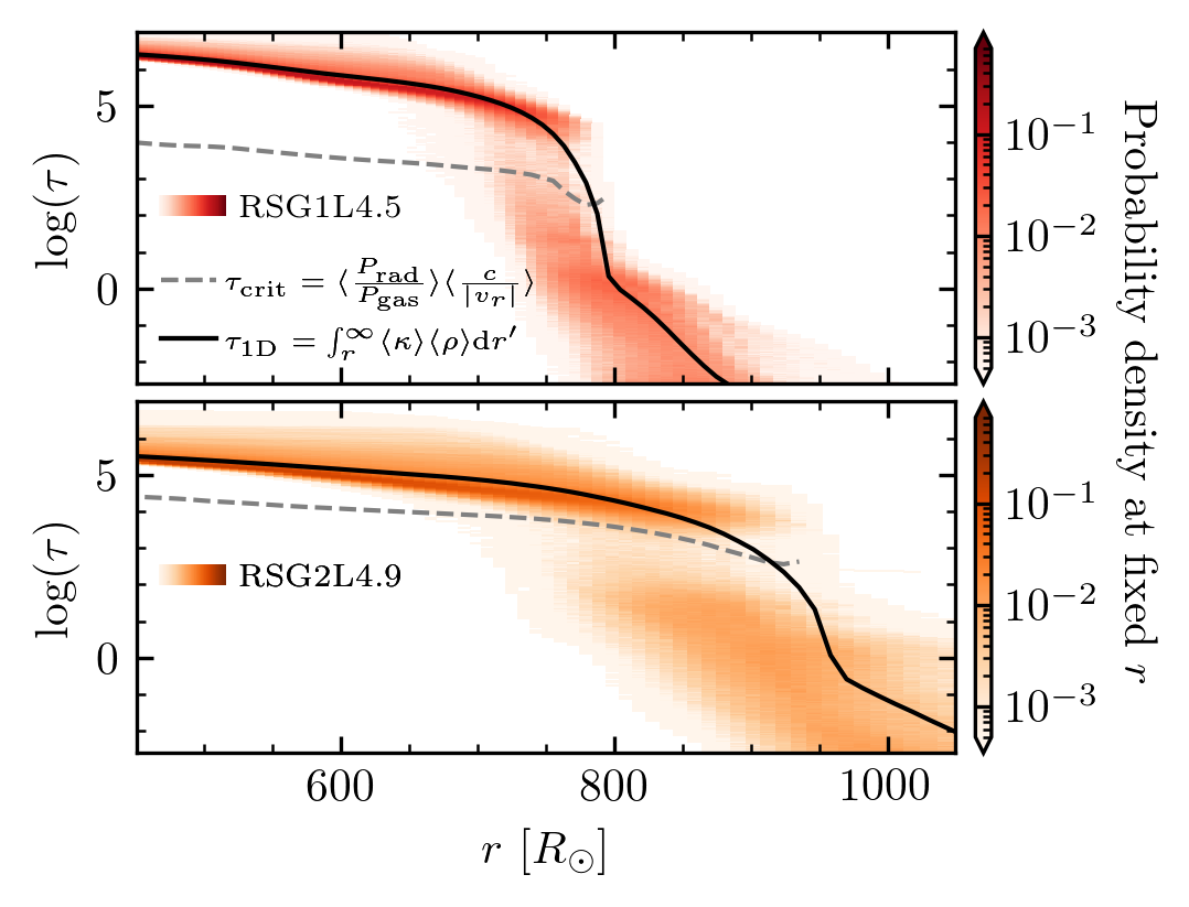
Figure 16: Optical depth $\tau$ in characteristic snapshots of our RSG1L4.5 (day 4707; red, upper panel) and RSG2L4.9 (day 4927; orange, lower panel) models. Color saturation indicates the volume-weighted probability of finding a fluid element at each radial coordinate with a given $\tau$, calculated along radial lines of sight. Optical depth $\tau_{\mathrm{1D}}$, integrating the volume-averaged opacity and volume-averaged density, is given by the black line. The grey dashed line indicates the average $\tau_{\mathrm{crit}}$ at each radius (truncated outside $r=R_{\mathrm{phot}}$); near the outer layers of the star, most material is either significantly above or below $\tau_{\mathrm{crit}}$, with little material with $\tau\approx\tau_{\mathrm{crit}}$.

Fig. 16 compares the optical depth profile integrated along radial lines of sight in our 3D Athena++ simulations to the critical optical depth $\tau_{\mathrm{crit}}$ where we use the amplitude of the radial velocity $|v_{r}|=\sqrt{v_{r}^{2}}$ as our proxy for $v_{c}$. Due to the bimodal opacity distribution of material above and below H-recombination, at a given radius near where $\tau_{\mathrm{1D}}=\tau_{\mathrm{crit}}$, there is very little material with $\tau$ near $\tau_{\mathrm{crit}}$. Rather, most of the fluid has $\tau\gg\tau_{\mathrm{crit}}$ by over an order of magnitude, or $\tau\ll\tau_{\mathrm{crit}}$ by more than an order of magnitude. This is yet another signature of the large-scale plume structure; within a given plume, the convective velocities are set nonlocally, and except at interfaces between plumes there is little opportunity for radiative losses as fluid interacts primarily within the same plume. Comparing to the same snapshots in Fig. 11, while the entropy profiles begin to decline due to superadiabatic convection even where $\tau>\tau_{\mathrm{crit}}$ (especially in the more luminous RSG2L4.9 model), the entropy profiles decline significantly in the region where some material has $\tau<\tau_{\mathrm{crit}}$, due to the plumes losing heat via diffusion and, where $\tau\mathrel{\vbox{ \offinterlineskip\halign{\hfil$#$\cr<\cr\kern 2.0pt\cr\sim\cr\kern-2.0pt\cr}}}1$, non-local radiative losses.

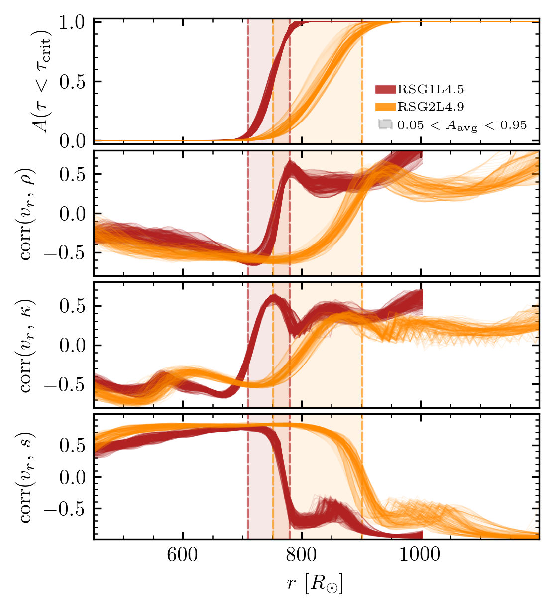
Figure 17: Fraction of the solid angle where $\tau<\tau_{\mathrm{crit}}$ along a radial line of sight (top panel), as well as the correlations of radial velocity with the density (second panel), opacity (third panel), and entropy (bottom panel). Colored lines show $\approx 350$ total snapshots starting from day 4000 in RSG1L4.5 and day 4500 in RSG2L4.9, until the end of the simulations. The shaded area indicates radii where the time-average of $A(\tau<\tau_{\mathrm{crit}})$ is between 5% and 95%. The RSG1L4.5 data are truncated at $r=1000R_{\odot}$, where the density approaches the density floor.

At optical depths with radiation-dominated energy transport where $\tau<\tau_{\mathrm{crit}}$, but still $\tau>1$, radiation forces may significantly impact fluid motion at high $L\sim L_{\mathrm{Edd}}$. In our simulations, we observe a change in the dynamics between regions of high and low $\tau/\tau_{\mathrm{crit}}$. This change can be seen in Fig. 17, which shows the area fraction of material with $\tau<\tau_{\mathrm{crit}}$, compared to correlations between the radial velocity and the density, opacity, and entropy of the fluid, defined by

$$\mathrm{corr}(x,y)=\frac{\sum\left(x_{i}-\langle{x}\rangle\right)\left(y_{i}-\langle{y}\rangle\right)}{\sqrt{\sum\left(x_{i}-\langle{x}\rangle\right)^{2}\sum\left(y_{i}-\langle{y}\rangle\right)^{2}}}$$ (10)

and the sum is taken over all zones (subscript $i$) in each radial shell. Where $A(\tau<\tau_{\mathrm{crit}})=0$, the density and opacity are anti-correlated with the radial velocity, and the entropy is positively correlated with the radial velocity (where +$v_{r}$ is defined as moving outwards). This is as expected for typical MLT-like convection; the material that sinks is denser, lower-entropy (colder), and more opaque material than the surrounding medium. However, for the outer radii where $\tau<\tau_{\mathrm{crit}}$, the correlation switches and cold (low-entropy), opaque, dense regions rise! The shaded area indicates radii where the fluid shows a mix of $\tau>\tau_{\mathrm{crit}}$ and $\tau<\tau_{\mathrm{crit}}$ material, quantified by where the time-average of $A(\tau<\tau_{\mathrm{crit}})$ is between 5% and 95%, and it also captures the region in the star where the correlations invert. This inverted correlation is also characteristic of surface turbulence driven by the Fe opacity peak in younger massive stars (Schultz et al., in prep). In these highly luminous stars, $L$ can exceed $L_{\mathrm{Edd}}$ at the $\tau=\tau_{\mathrm{crit}}$ location due to the presence of opacity peaks, and further analysis is required to understand what drives these near-surface dynamics. Because the nature the RHD turbulence changes where $\tau<\tau_{\mathrm{crit}}$, we thus presume for now that $\tau\approx\tau_{\mathrm{crit}}$ is an outer boundary where MLT treatments may cease to be appropriate in the RSG regime.

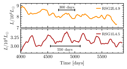
Figure 18: Lightcurves starting at day 4000 for both simulation runs. The RSG1L4.5 lightcurve is shown red on the lower panel and RSG2L4.9 in orange on the upper panel. Characteristic velocity decorrelation times for each model are indicated on the figure.

Moreover, the observable photosphere around $R_{\mathrm{phot}}$ is in this lossy, inverted-correlation, turbulent-pressure-dominated region! The convective motions here give rise to luminosity variations on timescales comparable to the timescales of the global convection cells. Fig. 18 shows the lightcurves of the last $\approx$2000 days of our simulations, determined at the simulation outer boundary as $L(t)=\frac{4\pi}{\Omega_{\mathrm{sim}}}\int r^{2}F_{r}(t)\mathrm{d}\Omega$, where $\Omega_{\mathrm{sim}}=\int_{\theta=\frac{\pi}{4}}^{\frac{3\pi}{4}}\int_{\phi=0}^{\pi}\mathrm{d}(\cos\theta)\mathrm{d}\phi$ is the solid-angle of our simulation domain. Fitting a second-order polynomial to the lightcurves and subtracting $L(t)-L_{\mathrm{poly}}(t)$, we compute the time-weighted variance as $\sigma_{L}^{2}=\sum{[L(t)-L_{\mathrm{poly}}(t)]^{2}\mathrm{d}t}/\sum\mathrm{d}t$, and the fluctuation amplitude as $\mathrm{max}[L(t)-L_{\mathrm{poly}}(t)]-\mathrm{min}[L(t)-L_{\mathrm{poly}}(t)]$. The lightcurves beyond day 4000 exhibit $\approx 3\%$ mean luminosity fluctuations, with $\sqrt{\sigma_{L}^{2}}=0.89\times 10^{3}L_{\odot}$ in RSG1L4.5, and $\sqrt{\sigma_{L}^{2}}=1.9\times 10^{3}L_{\odot}$ in RSG2L4.9. Fluctuation amplitudes are $\approx$10%: $3.6\times 10^{3}L_{\odot}$ in RSG1L4.5 and $8.6\times 10^{3}L_{\odot}$ in RSG2L4.9. The peak-to-peak fluctuations in the lightcurves are irregular in time, and for RSG2L4.9 a single dominant period could not be found in the power spectrum. This is likely due to the stochastic nature of the convective fluctuations. For the de-trended RSG1L4.5 power spectrum calculated from day 4500 onward, there is some excess power centered around 310 days/cycle with a 70 day spread resembling quasi-periodic oscillations with a wide window function. This flattens out when considering the lightcurve after day 4000, and disappears when considering the lightcurve from much earlier than that. We discuss briefly in the Conclusions (§6) how this variability compares to observations.

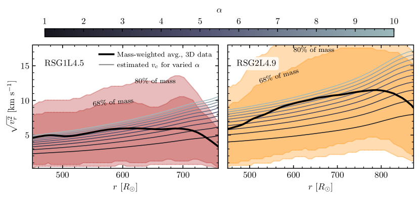
Figure 19: Radial fluid velocity magnitudes at characteristic snapshots of our models compared to MLT. The left panel shows RSG1L4.5 at day 4707, and the right panel shows RSG2L4.9 at day 4927. Mass-weighted average velocities are shown as thick black lines, with 68% and 80% of the mass lying within the dark and light shaded regions, respectively. The grey lines indicate the convective velocities predicted from MLT given the volume-averaged temperature and density profiles and the model luminosity, for integer values of $\alpha=1-10$. The plots are truncated where $\mathrm{corr}(v_{r},\rho)=0$, outside of which the turbulent motions do not resemble MLT-like convection.

4.5 Caveats of the 3D models

There are a few caveats which we believe do not impact any of the results presented here, but are worth stating. First, while we include radiation pressure in the stellar interior, the radiation transport module in Athena++ is not yet compatible with arbitrary gas equations of state. As such, our assumed value of $\mu=0.645$ entails that the gas pressure may be overestimated by up to a factor of $2$ in the outer regions with $T\mathrel{\vbox{ \offinterlineskip\halign{\hfil$#$\cr<\cr\kern 2.0pt\cr\sim\cr\kern-2.0pt\cr}}}10^{4}$K, which could help account for the relatively low $T_{\mathrm{eff}}$ of our models. However, it should be noted that this region is exactly where turbulent pressure is expected to dominate over thermal pressure, which would be even more significant if the gas pressure were lower than in our models here due to H recombination. Secondly, while these simulations employ full self-consistent coupling between radiation and hydrodynamics, the grey OPAL opacities do not account for frequency-dependent effects. As shown by Chiavassa et al. (2011a), non-grey opacities could lead to a steeper thermal gradient in the optically thin region, with weaker temperature fluctuations, which affects the stellar spectrum and thereby interferometric determinations of stellar radii. The small changes in the mass within the simulation domain are dominated by IB effects and not outflows. The incorporation of non-grey phenomena would also be required to place first-principles constraints on mass loss and other important observable stellar properties. Finally, while our simulation domain captures a very large fraction of the $\Omega=2\pi$ hemisphere, the relatively few convective plumes suggest that a full $\Omega=4\pi$ simulation might yield more accurate cancellation of random angular momenta than our estimate, and may have an impact on the RSG lightcurve, which shows variability consistent with these stochastic convective fluctuations.

5 Implications for 1D calculations

Computational RHD models of convection enable tests of MLT assumptions, possible calibrations, and incorporation into 1D models. A fundamental set of early 2D RHD simulations (Ludwig et al., 1999) calibrated MLT parameters for portions of the low-optical-depth regime in $L\ll L_{\mathrm{Edd}}$ stars, which was followed up with 3D simulations by Sonoi et al. (2019), who do not definitively conclude if any particular convection model gives the best correspondence between 1D and 3D models, but constrain $\alpha\approx 1-2$ across a grid of cool giant atmospheres (Red Giants with $T_{\mathrm{eff}}>4000$K), in agreement with some observational constraints (e.g. Joyce & Chaboyer, 2018). Other works (e.g. Trampedach et al. 2014b; Magic et al. 2015; Salaris & Cassisi 2015) recovered similar calibrations in similar $L\ll L_{\mathrm{Edd}}$ stars, though as convection becomes more vigorous in stars with higher luminosity and stronger opacity peaks and plumes take up larger and larger fractions of the star, the convective motions, particularly at the stellar surface, can deviate significantly from MLT (see e.g. discussion in Trampedach et al., 2013). We now discuss the implications of our 3D models for 1D calculations, focusing on the region where $\mathrm{corr}(v_{r},\rho)<0$ so convection can be fairly compared to MLT’s working hypothesis. Hereafter, we will refer to the location where the $v_{r}-\rho$ correlation inverts $(\mathrm{corr}(v_{r},\rho)=0)$ as the “correlation radius,” $R_{\mathrm{corr}}$.

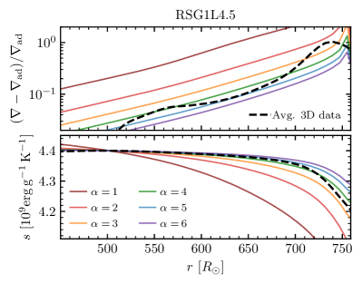
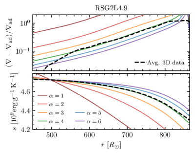
Figure 20: Comparison of superadiabaticity (upper panels) and specific entropy (lower panels) derived from our 3D models (black dashed lines) and from MLT (solid colored lines), for RSG1L4.5 (left) and RSG2L4.9 (right) when $P_{\mathrm{turb}}$ is neglected. All values shown are derived from the time-averaged, shellular (volume-weighted) averaged density and temperature profiles, as well as the time-averaged luminosity at the simulation outer boundary, beyond day 4000 in RSG1L4.5 and beyond day 4500 in RSG2L4.9.

5.1 Comparing Convective Velocities to MLT Expectations

We first check the fluid velocities in our models against expectations from MLT for spherical stellar envelopes with luminosity $L$, and $\rho(r)$, and $T(r)$ profiles matching averages of our 3D models. Where convection carries most of the flux, as in the RSG interior, $F_{\mathrm{conv}}\approx L/4\pi r^{2}$, and from Eqs (2) and (3),

$$v_{c}\approx\left(\frac{\alpha}{4}\right)^{1/3}\left(\frac{L}{4\pi r^{2}}{\frac{PQ}{\rho^{2}c_{p}T}}\right)^{1/3}.$$ (11)

Fig. 19 compares this expectation to the fluid motion in our two RSG envelope models as a function of the mixing length parameter $\alpha$, with the diagnostic velocity taken to be $\sqrt{v_{r}^{2}}$ in the 3D models. We represent the 3D data via bands, with 80% of the mass having velocities lying within the light colored regions, and 68% having velocities within the darker colored regions. The mass-weighted averages are indicated by the thick black lines. For clarity, we show here the comparison for individual model snapshots; the time-averaged profiles display similar behavior. The azimuthal and polar velocity profiles are comparable, with $\langle\sqrt{v_{\theta}^{2}}\rangle_{m}\approx\langle\sqrt{v_{\phi}^{2}}\rangle_{m}\approx 5-8$ km/s in RSG1L4.5 and 7-9 km/s in RSG2L4.9, with large scatter ($\mathrel{\vbox{ \offinterlineskip\halign{\hfil$#$\cr>\cr\kern 2.0pt\cr\sim\cr\kern-2.0pt\cr}}}\pm 5$km/s), and radial motion accounts for $\approx 1/3-1/2$ of the turbulent kinetic energy density. We see good (factor of $\approx 2$) agreement between the convective velocities predicted by MLT and the 3D models, and the scatter in convective velocities is much larger than the factor of $10^{1/3}$ introduced by varying $\alpha$ by a factor of 10. In both models, the velocity profile is flatter across a larger radial domain than MLT would predict for a fixed $\alpha$. We speculate that this can be attributed to the nonlocal, large-scale nature of the plumes, as the velocity profile is set by the motion of a mixture of plumes which do not change significantly over the simulation domain; this is also noted in, e.g., Brun & Palacios (2009) in 3D simulations of RGB stars.

5.2 Calibration of Mixing Length Parameters in the Absence of $P_{\mathrm{turb}}$

Convective efficiency is important in determining the stellar radius as discussed in detail in §2; therefore it is valuable to have a first-principles calibration of mixing length parameters, especially $\alpha$, within the RSG regime motivated by 3D models. Because the nature of the turbulent energy and momentum transport changes outside $R_{\mathrm{corr}}$, we treat $R_{\mathrm{corr}}$ as an outer boundary beyond which MLT treatments cannot be calibrated, and perhaps cease to be appropriate, in the high-luminosity RSG regime.

Most 1D stellar-evolutionary models do not account for turbulent pressure, and when included, it is a challenge (see discussion in Trampedach et al. 2014b), so we first explore the case where $P=P_{\mathrm{therm}}=P_{\mathrm{rad}}+P_{\mathrm{gas}}$. We generate a 1D model from the 3D simulations by finding the time-averaged, volume-averaged radial density and temperature profiles from each 3D simulation run ($\rho_{\mathrm{1D}}(r)$ and $T_{\mathrm{1D}}(r)$, respectively). We choose volume-averages along surfaces of constant gravity (radial coordinates) due to the loosely-bound nature of the envelope, though where $r<R_{\mathrm{corr}}$ different averages do not significantly affect our results. We calculate $\kappa$ from these profiles using the OPAL tables. The total luminosity is taken to be the time-averaged luminosity in the outermost zone $L=L_{\mathrm{surf}}$, up to the end of the simulation starting from day 4000 in RSG1L4.5 and from day 4500 in RSG2L4.9. We assume an EOS of ideal gas + radiation with $\mu=0.645$, as in our 3D model, which is appropriate for $r<R_{\mathrm{corr}}$ as $T\mathrel{\vbox{ \offinterlineskip\halign{\hfil$#$\cr>\cr\kern 2.0pt\cr\sim\cr\kern-2.0pt\cr}}}10^{4}$K. We then solve the Henyey et al. (1965) MLT equations assuming $y=3/4\pi^{2}$, and consider only material inside $R_{\mathrm{corr}}$ (where $\tau>\tau_{\mathrm{crit}}\gg 1$) for different values of $\alpha$ (see Appendix A for more specific details).

The upper panels of Fig. 20 show the comparison between the superadiabaticity, expressed as $(\nabla-\nabla_{\mathrm{ad}})/\nabla_{\mathrm{ad}}$, using $\nabla$ predicted by MLT and $\nabla$ derived directly from the averaged 3D data. The x-axis limits are $450R_{\odot}$ and $R_{\mathrm{corr}}$, respectively. We see significant deviations between $\nabla$ from $\nabla_{\mathrm{ad}}$, with nearly-adiabatic behavior in the interior and increasing superadiabaticity outward. The lower panels show entropy profiles, which are often used to calibrate MLT parameters to 3D atmosphere models in more compact, less luminous stellar environments (e.g. Trampedach et al., 2014b; Magic et al., 2015; Magic, 2016; Sonoi et al., 2019). For our averaged 3D data, we calculate $s$ including radiation and gas entropy, $s=\frac{k_{\mathrm{B}}}{\mu m_{p}}\ln\left(T^{3/2}/\rho\right)+\frac{4}{3}a_{r}T^{3}/\rho$, where $T$ is in K and $\rho$ is in g/cm³, and for MLT we integrate $\mathrm{d}s=c_{P}\,\mathrm{d}\ln T\left[1-\nabla_{\mathrm{ad}}/\nabla\right]$ using $\nabla$ given by MLT, connecting to the nearly-adiabatic $r=500R_{\odot}$ location to ensure agreement in the additive constant. Both models display nice agreement with $\alpha=4$ in the interior. At larger radii, the RSG1L4.5 model (left panels) exhibits greater superadiabaticity than implied by $\alpha=4$, in better agreement with $\alpha=2-3$. This contributes to the entropy profile, which falls more steeply than $\alpha=4$ and approaches the value predicted by $\alpha=3$ in our region of consideration. The more luminous RSG2L4.9 model (right panels of Fig. 20) closely follows the $\alpha=4$ predictions throughout most of the domain of interest, with generally excellent agreement for the entropy profile, becoming more shallow as $r$ approaches $R_{\mathrm{corr}}$.

5.3 Estimating $P_{\mathrm{turb}}$ in a 1D model and MLT Implications

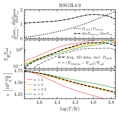
Figure 21: Impact of turbulent pressure on mixing length calibration. Comparison of superadiabaticity (middle panel) and entropy (lower panel) are shown, for our averaged 3D RSG2L4.9 model (black dashed lines) and MLT with different $\alpha$ (solid colored lines) as a function of temperature. The upper panel shows $P_{\mathrm{turb}}/P_{\mathrm{therm}}$ (dotted line) and $\mathrm{d}\ln P_{\mathrm{therm}}/\mathrm{d}\ln P_{\mathrm{tot}}$ (dash-dot line), which are included in the MLT calculation and in the averaged 3D $\nabla$. The grey dashed line in the middle panel shows $\nabla_{\mathrm{therm}}=\mathrm{d}\ln T/\mathrm{d}\ln P_{\mathrm{therm}}$ to facilitate direct comparison to Fig. 20. All values shown are derived from the time-averaged (beyond day 4500), shellular (volume-weighted) averaged density, temperature, and kinetic energy profiles, as well as the time-averaged luminosity at the simulation outer boundary. The x-axis extends from $r=450R_{\odot}$ to $R_{\mathrm{corr}}=865R_{\odot}$.

In a vigorously convective stellar envelope, turbulent pressure can become comparable to the thermal pressure and provide hydrostatic support. A fully self-consistent 1D implementation of turbulent pressure in 1D models remains an open challenge, as the inclusion of turbulent pressure leads to unrealistically steep pressure gradients near convective boundaries, especially near the stellar surface (Trampedach et al., 2014b). In MLT, turbulent pressure can be incorporated by modifying the pressure scale height and the adiabatic temperature gradient. Using the chain rule to include $P_{\mathrm{tot}}=P_{\mathrm{turb}}+P_{\mathrm{therm}}$, the modified adiabatic temperature gradient, $\nabla_{\mathrm{ad}}^{\prime}$, is given by (Henyey et al., 1965),

$$\nabla_{\mathrm{ad}}^{\prime}=\left(\frac{\mathrm{d}\ln{T}}{\mathrm{d}\ln{P_{\mathrm{therm}}}}\right)_{\mathrm{ad}}\times\frac{\mathrm{d}\ln{P_{\mathrm{therm}}}}{\mathrm{d}\ln{P_{\mathrm{tot}}}}.$$ (12)

The substitution $\nabla_{\mathrm{ad}}\rightarrow\nabla_{\mathrm{ad}}^{\prime}$ is then made where $\nabla_{\mathrm{ad}}$ appears in the MLT equations (Henyey et al. 1965; see also our Appendix B) and $H$ is calculated as $P_{\mathrm{tot}}/\rho g$. The lack of a reliable method to estimate $P_{\mathrm{turb}}$ inhibits such an incorporation in most 1D MLT implementations. For convenience, definitions of different gradients we used are also summarized in Appendix B.

Quantifying the pressure associated with turbulent kinetic energy densities from 3D RHD models allows us to explore how the 1D gradients are modified for these stars. The nonlocal nature of the convective motions means that the characteristic fluid velocity used in calculating $P_{\mathrm{turb}}$ is not simply identified with the velocity parameter in MLT. Therefore, in order to estimate the impact of turbulent pressure on the thermodynamic gradients and recovered values of $\alpha$, we determine $\mathrm{d}\ln P_{\mathrm{therm}}/\mathrm{d}\ln P_{\mathrm{tot}}$ directly from 1D averages of our 3D models. For this initial exploration, we calculate $P_{\mathrm{turb}}$ and thereby $\mathrm{d}\ln P_{\mathrm{therm}}/\mathrm{d}\ln P_{\mathrm{tot}}$ using the time-average of the angle-averaged $P_{\mathrm{turb}}=\langle\rho v_{r}v_{r}\rangle$. We then use Henyey et al. (1965)’s formula with turbulent pressure motivated by the 3D data to solve for $\nabla$ at different values of $\alpha$.

Fig. 21 shows the results of this exercise for the RSG2L4.9 model. The upper panel shows the adiabatic correction term ($\mathrm{d}\ln P_{\mathrm{therm}}/\mathrm{d}\ln P_{\mathrm{tot}}$; dash-dot line), as well as the ratio of turbulent pressure to thermal pressure (dotted line). The value of $\nabla=\mathrm{d}\ln T/\mathrm{d}\ln P_{\mathrm{tot}}$ from the averaged 3D data, for which we now include turbulent pressure as $P_{\mathrm{tot}}=P_{\mathrm{therm}}+P_{\mathrm{turb}}$, is shown by the black dashed line in the middle panel. For direct comparison to Fig. 20, we compare $\nabla$ here to $\nabla_{\mathrm{ad}}$ rather than $\nabla_{\mathrm{ad}}^{\prime}$. To further facilitate direct comparison, the grey dashed line in the middle panel shows the value of $\nabla_{\mathrm{therm}}=\mathrm{d}\ln{T}/\mathrm{d}\ln{P_{\mathrm{therm}}}$, which was taken to be equivalent to the true $\nabla$ in §5.2 and is equivalent to the dashed black line in the upper right panel of Fig. 20. The lower panel shows the entropy, calculated using $\nabla_{\mathrm{ad}}^{\prime}$ and $\nabla$. The black dashed line in the lower panel gives the entropy profile for our 3D-motivated 1D model, which is equivalent to the black dashed line in the lower right panel in Fig. 20, as the turbulent pressure terms cancel in the expression for $s$ (i.e. $\nabla_{\mathrm{ad}}^{\prime}/\nabla=\nabla_{\mathrm{ad}}/\nabla_{\mathrm{therm}}$). For the MLT values, shown by the colored lines, each value of $\alpha$ recovers a larger value of $\nabla$ compared to §5.2, but a slightly shallower $s$ profile (as the turbulent pressure correction in $\nabla_{\mathrm{ad}}^{\prime}$ accounts for a greater portion of the $\nabla-\nabla_{\mathrm{ad}}$ excess). Therefore, if a 1D stellar evolution code were to include a turbulent pressure correction to MLT using the Henyey et al. (1965) parameters, we would recommend a value of $\alpha=3.2$ from this model.

6 Discussion & Conclusions

We have constructed global 3D radiation hydrodynamical simulations in the RSG regime which include an accurate gravitational potential and radiation pressure in the convective interior for the first time. These simulations span $\approx$70% of the $2\pi$ hemisphere and yield predictions for the turbulent structure and dynamics from the middle of the convective envelope out beyond the photosphere. Our incorporation of radiation pressure in optically thick regions has enabled realization of the expected nearly-constant entropy profile and convective-luminosity domination in the convective interior. In agreement with Freytag et al. (2002) and Chiavassa et al. (2009) we find that the convection is dominated by a few large-scale plumes which flow through most of the simulation domain and survive for timescales of $\approx$300 and $\approx$550 days (for RSG1L4.5 and RSG2L4.9, respectively; see Fig. 8). When the models reach a convective steady state, RSG1L4.5 has $\log(L/L_{\odot})\approx 4.5$ and $R_{\mathrm{phot}}\approx 800R_{\odot}$, and RSG2L4.9 has $\log(L/L_{\odot})\approx 4.9$ and $R_{\mathrm{phot}}\approx 900R_{\odot}$.

Both models display $\approx$10% variation in luminosity owing to the large-scale turbulent surface structure (see Fig. 18). Temporal observations (see, e.g. Kiss et al. 2006; Soraisam et al. 2018; Conroy et al. 2018; Chatys et al. 2019; Ren et al. 2019; Soraisam et al. 2020) reveal RSG variability on timescales of a few hundred to thousands of days in a variety of host environments. These signals include both periodic and stochastic behavior, with increasing ubiquity of larger-amplitude fluctuations for brighter stars. In M31, for example, all RSGs brighter than $\log(L/L_{\odot})>4.8$ display lightcurve fluctuations with $\Delta m_{R}>0.05\ \mathrm{mag}$, up to around $\Delta m_{R}\approx 0.4$ (Soraisam et al., 2018). Periodic variability is interpreted as radial pulsations (Stothers, 1969; Stothers & Leung, 1971; Guo & Li, 2002), likely driven by a hydrogen ionization region inside the convective envelope (Heger et al., 1997; Yoon & Cantiello, 2010). The stochastic fluctuations (e.g. Ren & Jiang, 2020) qualitatively agree with our models, and we intend further analysis to compare these convective models directly to observations.

In the outer stellar layers, radiation carries an increasing fraction of the total luminosity as convection becomes lossy. This transition is associated with reaching an optical depth $\tau<\tau_{\mathrm{crit}}\approx 100$. Moreover, large density fluctuations and appreciable bimodality in $\kappa$ and $T$ lead to a range of radii with increasing amounts of material at $\tau<\tau_{\mathrm{crit}}$ (see Figs. 15,16). In the region where $\tau$ along some lines of sight falls below $\tau_{\mathrm{crit}}$, the correlations of radial velocity with the fluid density, entropy, and opacity fluctuations invert from what is characteristic of convective fluid motions (see Fig. 17); indeed the denser, lower-entropy, higher-opacity material rises! These inverse correlations at $A(\tau<\tau_{\mathrm{crit}})<1$ where $L$ locally exceeds $L_{\mathrm{Edd}}$ will not be seen if radiation pressure is not inlcuded. The change in the nature of convective motions in the outermost stellar layers of these highly luminous RSGs also prohibits a comparison to MLT treatments. Hence, we define the radius where these correlations invert as $R_{\mathrm{corr}}$, taking it as an outer boundary where MLT-like treatments cease to be appropriate.

Inside $R_{\mathrm{corr}}$, where MLT is applicable, the velocity profiles are flatter than MLT-like convection due to the nonlocal, large-scale convective plumes, but display good order-of-magnitude agreement (see Fig. 19). By comparing entropy profiles and superadiabatic gradients inside $R<R_{\mathrm{corr}}$, we find from our 3D simulations that the mixing length $\alpha$ appropriate for convection in this regime is $\alpha\approx 3-4$ (see Fig. 20 for models which neglect pressure from the turbulent motions and Fig. 21 which includes an estimate for such a correction). This convective efficiency is more consistent with estimates of larger-than-solar mixing lengths from the HR position of RSG populations (Chun et al., 2018), supernova color evolution (Dessart et al., 2013), and even some 3D treatments of the Sun which compare conventional MLT to other prescriptions for handling the different flux terms (e.g. Porter & Woodward, 2000). Future work of immediate interest will focus on better understanding the nature and implications of the surface turbulence outside of $R_{\mathrm{corr}}$. Similar inverted-correlation behavior is also seen in other simulations of luminous stars (e.g. in OB-star envelopes; Schultz et al. (2022)), but not in simulations of solar-like convection (e.g. Stein & Nordlund 1998), and may owe to RHD effects where $\tau_{\mathrm{crit}}\gg 1$ and $L\mathrel{\vbox{ \offinterlineskip\halign{\hfil$#$\cr>\cr\kern 2.0pt\cr\sim\cr\kern-2.0pt\cr}}}L_{\mathrm{Edd}}$.

In addition to exhibiting large density fluctuations which increase at large radii, the Athena++ RSG models display shallower density profiles in their outer stellar halos compared to traditional 1D hydrostatic models, and material near $\tau=1$ ($\approx$50$-$100$R_{\odot}$ beyond $R_{\mathrm{corr}}$) reaches densities 1 – 2 orders of magnitude lower than barren 1D model photospheres. In the eventual explosion of a RSG as a Type IIP Supernova, shock propagation (and therefore the SN emission) may be moderated by these 3D envelopes. Early SN emission (first $\approx 30$ days) is sensitive to the outermost $<0.01-0.1M_{\odot}$ of material; thus the inverted-correlation surface-turbulent outer halo defines the emitting region for the shock breakout and shock cooling phases of SN evolution. These phases have been studied extensively for 1D hydrostatic models with a well-defined outer radius (e.g., Nakar & Sari 2010; Morozova et al. 2016; Shussman et al. 2016; Sapir & Waxman 2017; Faran & Sari 2019; Kozyreva et al. 2020), but not for fundamentally 3D envelopes. The outer halo of material will also modify the predicted UV shock breakout signatures. The extent to which the 3D envelope properties discussed above may aid in our understanding of early-time Type IIP SN emission is thus an exciting avenue for our future exploration.

Appendix A MLT Calibration Details and Sensitivities

In MLT, as deployed by Henyey et al. (1965), the optical thickness of a bubble is $\omega=\kappa\rho\ell$, akin to $\tau_{\mathrm{b}}$ discussed in §4.4, which is typically comparable to the optical depth to the surface ($\tau$) when the opacity is not changing drastically. The convective efficiency parameter is then given by

$$\gamma=\frac{\nabla-\nabla_{\mathrm{e}}}{\nabla_{\mathrm{e}}-\nabla_{\mathrm{ad}}}=\gamma_{0}v_{c}$$ (A1)

where $\gamma_{0}=c_{p}\rho/\left(8\sigma_{\mathrm{SB}}T^{3}\theta\right)$, $\theta=\omega/(1+y\omega^{2})$, and $y$ depends on the geometry of the bubble. We solve for $\gamma$ via the cubic equation

$$\gamma+\gamma^{2}+\phi\gamma^{3}=\frac{gHQ\left(\alpha\gamma_{0}^{2}\right)}{\nu}\left(f\nabla_{\mathrm{rad}}-\nabla_{\mathrm{ad}}\right),$$ (A2)

where $F=L_{\mathrm{surf}}/4\pi r^{2}=16\sigma T^{4}\nabla_{\mathrm{rad}}/3\kappa\rho H$ defines $\nabla_{\mathrm{rad}}$ as the gradient required to carry all flux by radiative diffusion, $\phi=\frac{3}{4}f\omega\theta$, $\nu=8$, and $f=1$ as $\tau>\tau_{\mathrm{crit}}\gg 1$ inside $R_{\mathrm{corr}}$. For an ideal gas + radiation, EOS properties vary with $\alpha_{P}\equiv P_{\mathrm{rad}}/P_{\mathrm{gas}}$ (Mihalas & Mihalas 1984; $P$ subscript added to distinguish from $\alpha=\ell/H$), with

$$c_{P}=\frac{5}{2}\frac{k_{B}}{\mu m_{p}}\left(1+8\alpha_{P}+\frac{32}{5}\alpha_{P}^{2}\right),$$ (A3)

and

$$\nabla_{\mathrm{ad}}=\frac{1+5\alpha_{P}+4{\alpha_{P}}^{2}}{\frac{5}{2}+20\alpha_{P}+16{\alpha_{P}}^{2}}.$$ (A4)

From this, MLT yields a prediction for $\nabla$, which we compare to the gradients derived from $\rho_{\mathrm{1D}}$ and $T_{\mathrm{1D}}$:

$$\nabla=\frac{(1+\gamma)f\nabla_{\mathrm{rad}}+\phi\gamma^{2}\nabla_{\mathrm{ad}}}{1+\gamma+\phi\gamma^{2}}.$$ (A5)

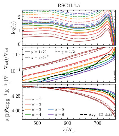
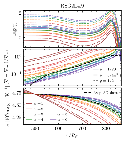
Figure 22: Comparison of efficiency factor $\gamma$ (upper panels), superadiabaticity (middle panels) and entropy (lower panels) derived from our 3D models (black dashed lines) and from MLT (pastel colored lines) against profiles derived from RSG1L4.5 (left) and RSG2L4.9 (right) when $P_{\mathrm{turb}}$ is neglected. Each color corresponds to a different value of $\alpha$, and each linestyle (solid, dash-dot, dashed) corresponds to a different value of $y$.

Following Henyey et al. (1965), we use $y=3/4\pi^{2}$ for our analysis in §5. We repeated this analysis varying $y$ for values ranging from $1/20$, which is the prediction for a parabolic temperature distribution inside a bubble, to $1/2$ (as used by Böhm-Vitense (1958)) which corresponds to a linear temperature distribution (see discussion in Henyey et al., 1965). This is shown in Fig. 22. The region inside $r<R_{\mathrm{corr}}$ is in the limit of higher $\omega$ ($\tau\gg 1$), so $\gamma_{0}\mathrel{\vbox{ \offinterlineskip\halign{\hfil$#$\cr\propto\cr\kern 2.0pt\cr\sim\cr\kern-2.0pt\cr}}}y$, leading to a strong $y$-dependence in $\gamma$ for both models. However, variations in $\gamma$ lead to large differences in $\nabla$ and $s$ only when $\gamma\mathrel{\vbox{ \offinterlineskip\halign{\hfil$#$\cr<\cr\kern 2.0pt\cr\sim\cr\kern-2.0pt\cr}}}1$. For the RSG1L4.5-derived model, $\omega$ is sufficiently large due to the slightly larger envelope mass and smaller radius, so fractional changes in $\gamma$ do not lead to significant differences in $\nabla$ or the recovered entropy profile except for the $\alpha=1$ line (which disagrees with the model profiles). In the case of RSG2L4.9, $\omega$ is smaller due to the lower envelope density, so changes in $y$ do affect the recovered superadiabatic gradient and entropy profiles even for $\alpha\mathrel{\vbox{ \offinterlineskip\halign{\hfil$#$\cr<\cr\kern 2.0pt\cr\sim\cr\kern-2.0pt\cr}}}3$, with higher values of $y$ leading to smaller $\nabla-\nabla_{\mathrm{ad}}$ and flatter $s$ profiles. However, this effect is still not substantial for $\alpha=4$, which also agrees best with the model. In all cases, the variation in $\nabla$ and $s$ introduced by varying $y$ is dominated by differences with different $\alpha$.

Comparing the luminosity carried by radiation recovered by MLT to the time-averaged shell-averaged $F_{r}$ of the 3D models, there is good agreement between the MLT values in both models within $\approx$5% for $r\mathrel{\vbox{ \offinterlineskip\halign{\hfil$#$\cr<\cr\kern 2.0pt\cr\sim\cr\kern-2.0pt\cr}}}700R_{\odot}$. Outside of those locations, however, MLT predicts dramatically lower radiative fluxes and higher convective fluxes due to the presence of the H opacity peak. This is not surprising for two reasons. First, we consider $\kappa$ from a 1D OPAL call, where the H opacity spike is sharper (see the bottom panels of Fig. 15) compared to the 3D data which displays a bimodal distribution of $\kappa$ in a given radial shell. Secondly, different values of $\tau$ along different lines of sight where there is appreciable bimodality (see Figs. 15,16) allow radiation to carry more of the flux than one would expect from radiative diffusion through a 1D shell with no density fluctuations.

Appendix B Gradient Definitions with and without Turbulent Pressure

For convenience, we state here how the above equations include the Henyey et al. (1965) turbulent-pressure correction. When $P_{\mathrm{tot}}=P_{\mathrm{therm}}+P_{\mathrm{turb}}$ is included, the modified Eq. A1 is

$$\gamma=\frac{\nabla-\nabla_{\mathrm{e}}}{\nabla_{\mathrm{e}}-\nabla_{\mathrm{ad}}^{\prime}}=\gamma_{0}v_{c},$$ (B1)

Eq. A2 becomes

$$\gamma+\gamma^{2}+\phi\gamma^{3}=\frac{gHQ\left(\alpha\gamma_{0}^{2}\right)}{\nu}\left(f\nabla_{\mathrm{rad}}-\nabla_{\mathrm{ad}}^{\prime}\right),$$ (B2)

and Eq. A5 becomes

$$\nabla=\frac{(1+\gamma)f\nabla_{\mathrm{rad}}+\phi\gamma^{2}\nabla_{\mathrm{ad}}^{\prime}}{1+\gamma+\phi\gamma^{2}}.$$ (B3)

For clarity, the definitions of the relevant gradients are given in Table 2 (on the next page).

gradient	Definition
$\nabla$	actual $\frac{\mathrm{d}\ln T}{{\mathrm{d}\ln P}}$ in the star
$\nabla_{\mathrm{therm}}$	$\frac{\mathrm{d}\ln T}{{\mathrm{d}\ln P_{\mathrm{therm}}}}$ in the star
$\nabla_{\mathrm{e}}$	$\nabla$ inside an eddy as it moves
$\nabla_{\mathrm{ad}}$	$\left(\frac{\mathrm{d}\ln T}{{\mathrm{d}\ln P_{\mathrm{therm}}}}\right)_{\mathrm{ad}}$ from the fluid properties
$\nabla_{\mathrm{ad}}^{\prime}$	$\nabla_{\mathrm{ad}}\times\frac{d\ln{P_{\mathrm{th}}}}{d\ln{P_{\mathrm{tot}}}}$
$\nabla_{\mathrm{rad}}$	$\nabla$ required to carry $L_{\mathrm{surf}}$ solely by radiative diffusion$=(3L_{\mathrm{surf}}\kappa\rho H)/(64\pi r^{2}\sigma_{\mathrm{SB}}T^{4})$

Table 2: Definitions of various gradients discussed in this work.

References

- Antoni & Quataert (2021) Antoni, A., & Quataert, E. 2021, arXiv e-prints, arXiv:2107.09068. https://arxiv.org/abs/2107.09068
- Arroyo-Torres et al. (2015) Arroyo-Torres, B., Wittkowski, M., Chiavassa, A., et al. 2015, A&A, 575, A50, doi: 10.1051/0004-6361/201425212
- Böhm-Vitense (1958) Böhm-Vitense, E. 1958, ZAp, 46, 108
- Brun & Palacios (2009) Brun, A. S., & Palacios, A. 2009, ApJ, 702, 1078, doi: 10.1088/0004-637X/702/2/1078
- Chatys et al. (2019) Chatys, F. W., Bedding, T. R., Murphy, S. J., et al. 2019, MNRAS, 487, 4832, doi: 10.1093/mnras/stz1584
- Chiavassa et al. (2018a) Chiavassa, A., Casagrande, L., Collet, R., et al. 2018a, A&A, 611, A11, doi: 10.1051/0004-6361/201732147
- Chiavassa et al. (2010a) Chiavassa, A., Collet, R., Casagrande, L., & Asplund, M. 2010a, A&A, 524, A93, doi: 10.1051/0004-6361/201015507
- Chiavassa et al. (2011a) Chiavassa, A., Freytag, B., Masseron, T., & Plez, B. 2011a, A&A, 535, A22, doi: 10.1051/0004-6361/201117463
- Chiavassa et al. (2018b) Chiavassa, A., Freytag, B., & Schultheis, M. 2018b, A&A, 617, L1, doi: 10.1051/0004-6361/201833844
- Chiavassa et al. (2010b) Chiavassa, A., Haubois, X., Young, J. S., et al. 2010b, A&A, 515, A12, doi: 10.1051/0004-6361/200913907
- Chiavassa et al. (2009) Chiavassa, A., Plez, B., Josselin, E., & Freytag, B. 2009, A&A, 506, 1351, doi: 10.1051/0004-6361/200911780
- Chiavassa et al. (2011b) Chiavassa, A., Pasquato, E., Jorissen, A., et al. 2011b, A&A, 528, A120, doi: 10.1051/0004-6361/201015768
- Chiavassa et al. (2017) Chiavassa, A., Norris, R., Montargès, M., et al. 2017, A&A, 600, L2, doi: 10.1051/0004-6361/201730438
- Chiavassa et al. (2020) Chiavassa, A., Kravchenko, K., Millour, F., et al. 2020, A&A, 640, A23, doi: 10.1051/0004-6361/202037832
- Chun et al. (2018) Chun, S.-H., Yoon, S.-C., Jung, M.-K., Kim, D. U., & Kim, J. 2018, ApJ, 853, 79, doi: 10.3847/1538-4357/aa9a37
- Conroy et al. (2018) Conroy, C., Strader, J., van Dokkum, P., et al. 2018, ApJ, 864, 111, doi: 10.3847/1538-4357/aad460
- Coughlin et al. (2018) Coughlin, E. R., Quataert, E., Fernández, R., & Kasen, D. 2018, MNRAS, 477, 1225, doi: 10.1093/mnras/sty667
- Cox & Giuli (1968) Cox, J. P., & Giuli, R. T. 1968, Principles of stellar structure
- Davies & Beasor (2018) Davies, B., & Beasor, E. R. 2018, MNRAS, 474, 2116, doi: 10.1093/mnras/stx2734
- Davies & Beasor (2020a) —. 2020a, MNRAS, 493, 468, doi: 10.1093/mnras/staa174
- Davies & Beasor (2020b) —. 2020b, MNRAS, 496, L142, doi: 10.1093/mnrasl/slaa102
- Dessart & Hillier (2019) Dessart, L., & Hillier, D. J. 2019, A&A, 625, A9, doi: 10.1051/0004-6361/201834732
- Dessart et al. (2013) Dessart, L., Hillier, D. J., Waldman, R., & Livne, E. 2013, MNRAS, 433, 1745, doi: 10.1093/mnras/stt861
- Dorch (2004) Dorch, S. B. F. 2004, A&A, 423, 1101, doi: 10.1051/0004-6361:20040435
- Dorn-Wallenstein et al. (2020) Dorn-Wallenstein, T. Z., Levesque, E. M., Neugent, K. F., et al. 2020, ApJ, 902, 24, doi: 10.3847/1538-4357/abb318
- Drout et al. (2012) Drout, M. R., Massey, P., & Meynet, G. 2012, ApJ, 750, 97, doi: 10.1088/0004-637X/750/2/97
- Ekström et al. (2012) Ekström, S., Georgy, C., Eggenberger, P., et al. 2012, A&A, 537, A146, doi: 10.1051/0004-6361/201117751
- Faran & Sari (2019) Faran, T., & Sari, R. 2019, ApJ, 884, 41, doi: 10.3847/1538-4357/ab3e3d
- Farmer et al. (2016) Farmer, R., Fields, C. E., Petermann, I., et al. 2016, ApJS, 227, 22, doi: 10.3847/1538-4365/227/2/22
- Freytag & Höfner (2008) Freytag, B., & Höfner, S. 2008, A&A, 483, 571, doi: 10.1051/0004-6361:20078096
- Freytag et al. (2017) Freytag, B., Liljegren, S., & Höfner, S. 2017, A&A, 600, A137, doi: 10.1051/0004-6361/201629594
- Freytag et al. (2002) Freytag, B., Steffen, M., & Dorch, B. 2002, Astronomische Nachrichten, 323, 213, doi: 10.1002/1521-3994(200208)323:3/4<213::AID-ASNA213>3.0.CO;2-H
- Freytag et al. (2012) Freytag, B., Steffen, M., Ludwig, H. G., et al. 2012, Journal of Computational Physics, 231, 919, doi: 10.1016/j.jcp.2011.09.026
- Freytag et al. (2010) Freytag, B., Steffen, M., Wedemeyer-Böhm, S., et al. 2010, CO5BOLD: COnservative COde for the COmputation of COmpressible COnvection in a BOx of L Dimensions with l=2,3. http://ascl.net/1011.014
- Fuller (2017) Fuller, J. 2017, MNRAS, 470, 1642, doi: 10.1093/mnras/stx1314
- Georgy et al. (2013) Georgy, C., Ekström, S., Eggenberger, P., et al. 2013, A&A, 558, A103, doi: 10.1051/0004-6361/201322178
- Glebbeek et al. (2009) Glebbeek, E., Gaburov, E., de Mink, S. E., Pols, O. R., & Portegies Zwart, S. F. 2009, A&A, 497, 255, doi: 10.1051/0004-6361/200810425
- Goldberg & Bildsten (2020) Goldberg, J. A., & Bildsten, L. 2020, ApJ, 895, L45, doi: 10.3847/2041-8213/ab9300
- Goldberg et al. (2019) Goldberg, J. A., Bildsten, L., & Paxton, B. 2019, ApJ, 879, 3, doi: 10.3847/1538-4357/ab22b6
- Goldberg et al. (2020) —. 2020, ApJ, 891, 15, doi: 10.3847/1538-4357/ab7205
- Guo & Li (2002) Guo, J. H., & Li, Y. 2002, ApJ, 565, 559, doi: 10.1086/324295
- Harris et al. (2020) Harris, C. R., Millman, K. J., van der Walt, S. J., et al. 2020, Nature, 585, 357–362, doi: 10.1038/s41586-020-2649-2
- Hauschildt et al. (1997) Hauschildt, P. H., Baron, E., & Allard, F. 1997, ApJ, 483, 390, doi: 10.1086/304233
- Heger et al. (1997) Heger, A., Jeannin, L., Langer, N., & Baraffe, I. 1997, A&A, 327, 224. https://arxiv.org/abs/astro-ph/9705097
- Henyey et al. (1965) Henyey, L., Vardya, M. S., & Bodenheimer, P. 1965, ApJ, 142, 841, doi: 10.1086/148357
- Hosseinzadeh et al. (2018) Hosseinzadeh, G., Valenti, S., McCully, C., et al. 2018, ApJ, 861, 63, doi: 10.3847/1538-4357/aac5f6
- Hunter (2007) Hunter, J. D. 2007, Computing in Science Engineering, 9, 90, doi: 10.1109/MCSE.2007.55
- Iglesias & Rogers (1996) Iglesias, C. A., & Rogers, F. J. 1996, ApJ, 464, 943, doi: 10.1086/177381
- Iglesias et al. (1992) Iglesias, C. A., Rogers, F. J., & Wilson, B. G. 1992, ApJ, 397, 717, doi: 10.1086/171827
- Jiang (2021) Jiang, Y.-F. 2021, ApJS, 253, 49, doi: 10.3847/1538-4365/abe303
- Jiang et al. (2015) Jiang, Y.-F., Cantiello, M., Bildsten, L., Quataert, E., & Blaes, O. 2015, ApJ, 813, 74, doi: 10.1088/0004-637X/813/1/74
- Jiang et al. (2018) Jiang, Y.-F., Cantiello, M., Bildsten, L., et al. 2018, Nature, 561, 498, doi: 10.1038/s41586-018-0525-0
- Jiang et al. (2014) Jiang, Y.-F., Stone, J. M., & Davis, S. W. 2014, ApJS, 213, 7, doi: 10.1088/0067-0049/213/1/7
- Joyce & Chaboyer (2018) Joyce, M., & Chaboyer, B. 2018, ApJ, 856, 10, doi: 10.3847/1538-4357/aab200
- Joyce et al. (2020) Joyce, M., Leung, S.-C., Molnár, L., et al. 2020, ApJ, 902, 63, doi: 10.3847/1538-4357/abb8db
- Kasen & Woosley (2009) Kasen, D., & Woosley, S. E. 2009, ApJ, 703, 2205, doi: 10.1088/0004-637X/703/2/2205
- Kippenhahn et al. (2013) Kippenhahn, R., Weigert, A., & Weiss, A. 2013, Stellar Structure and Evolution; 2nd ed., Astronomy and astrophysics library (Berlin: Springer), doi: 10.1007/978-3-642-30304-3. http://cds.cern.ch/record/1493272
- Kiss et al. (2006) Kiss, L. L., Szabó, G. M., & Bedding, T. R. 2006, MNRAS, 372, 1721, doi: 10.1111/j.1365-2966.2006.10973.x
- Kochanek (2020) Kochanek, C. S. 2020, MNRAS, 493, 4945, doi: 10.1093/mnras/staa605
- Kozyreva et al. (2020) Kozyreva, A., Nakar, E., Waldman, R., Blinnikov, S., & Baklanov, P. 2020, MNRAS, 494, 3927, doi: 10.1093/mnras/staa924
- Kravchenko et al. (2019) Kravchenko, K., Chiavassa, A., Van Eck, S., et al. 2019, A&A, 632, A28, doi: 10.1051/0004-6361/201935809
- Kravchenko et al. (2018) Kravchenko, K., Van Eck, S., Chiavassa, A., et al. 2018, A&A, 610, A29, doi: 10.1051/0004-6361/201731530
- Kravchenko et al. (2020) Kravchenko, K., Wittkowski, M., Jorissen, A., et al. 2020, A&A, 642, A235, doi: 10.1051/0004-6361/202038581
- Kravchenko et al. (2021) Kravchenko, K., Jorissen, A., Van Eck, S., et al. 2021, arXiv e-prints, arXiv:2104.08105. https://arxiv.org/abs/2104.08105
- Landau & Lifshitz (1987) Landau, L. D., & Lifshitz, E. M. 1987, Fluid Mechanics, Second Edition: Volume 6 (Course of Theoretical Physics), 2nd edn., Course of theoretical physics / by L. D. Landau and E. M. Lifshitz, Vol. 6 (Butterworth-Heinemann). http://www.worldcat.org/isbn/0750627670
- Levesque et al. (2006) Levesque, E. M., Massey, P., Olsen, K. A. G., et al. 2006, ApJ, 645, 1102, doi: 10.1086/504417
- Liljegren et al. (2018) Liljegren, S., Höfner, S., Freytag, B., & Bladh, S. 2018, A&A, 619, A47, doi: 10.1051/0004-6361/201833203
- Ludwig et al. (1999) Ludwig, H.-G., Freytag, B., & Steffen, M. 1999, A&A, 346, 111. https://arxiv.org/abs/astro-ph/9811179
- Magic (2016) Magic, Z. 2016, A&A, 586, A88, doi: 10.1051/0004-6361/201527438
- Magic et al. (2013a) Magic, Z., Collet, R., Asplund, M., et al. 2013a, A&A, 557, A26, doi: 10.1051/0004-6361/201321274
- Magic et al. (2013b) Magic, Z., Collet, R., Hayek, W., & Asplund, M. 2013b, A&A, 560, A8, doi: 10.1051/0004-6361/201322252
- Magic et al. (2015) Magic, Z., Weiss, A., & Asplund, M. 2015, A&A, 573, A89, doi: 10.1051/0004-6361/201423760
- Martinez & Bersten (2019) Martinez, L., & Bersten, M. C. 2019, A&A, 629, A124, doi: 10.1051/0004-6361/201834818
- Massey et al. (2021) Massey, P., Neugent, K. F., Levesque, E. M., Drout, M. R., & Courteau, S. 2021, AJ, 161, 79, doi: 10.3847/1538-3881/abd01f
- Massey & Olsen (2003) Massey, P., & Olsen, K. A. G. 2003, AJ, 126, 2867, doi: 10.1086/379558
- Meynet & Maeder (1997) Meynet, G., & Maeder, A. 1997, A&A, 321, 465
- Meynet et al. (2015) Meynet, G., Chomienne, V., Ekström, S., et al. 2015, A&A, 575, A60, doi: 10.1051/0004-6361/201424671
- Mihalas & Mihalas (1984) Mihalas, D., & Mihalas, B. W. 1984, Foundations of radiation hydrodynamics
- Montargès et al. (2021) Montargès, M., Cannon, E., Lagadec, E., et al. 2021, Nature, 594, 365, doi: 10.1038/s41586-021-03546-8
- Moriya et al. (2018) Moriya, T. J., Förster, F., Yoon, S.-C., Gräfener, G., & Blinnikov, S. I. 2018, MNRAS, 476, 2840, doi: 10.1093/mnras/sty475
- Morozova et al. (2020) Morozova, V., Piro, A. L., Fuller, J., & Van Dyk, S. D. 2020, ApJ, 891, L32, doi: 10.3847/2041-8213/ab77c8
- Morozova et al. (2016) Morozova, V., Piro, A. L., Renzo, M., & Ott, C. D. 2016, ApJ, 829, 109, doi: 10.3847/0004-637X/829/2/109
- Morozova et al. (2017) Morozova, V., Piro, A. L., & Valenti, S. 2017, ApJ, 838, 28, doi: 10.3847/1538-4357/aa6251
- Morozova et al. (2018) —. 2018, ApJ, 858, 15, doi: 10.3847/1538-4357/aab9a6
- Mosumgaard et al. (2018) Mosumgaard, J. R., Ball, W. H., Silva Aguirre, V., Weiss, A., & Christensen-Dalsgaard, J. 2018, MNRAS, 478, 5650, doi: 10.1093/mnras/sty1442
- Mosumgaard et al. (2020) Mosumgaard, J. R., Jørgensen, A. C. S., Weiss, A., Silva Aguirre, V., & Christensen-Dalsgaard, J. 2020, MNRAS, 491, 1160, doi: 10.1093/mnras/stz2979
- Nadezhin (1980) Nadezhin, D. K. 1980, Ap&SS, 69, 115, doi: 10.1007/BF00638971
- Nakar & Sari (2010) Nakar, E., & Sari, R. 2010, ApJ, 725, 904, doi: 10.1088/0004-637X/725/1/904
- Norris et al. (2021) Norris, R. P., Baron, F. R., Monnier, J. D., et al. 2021, arXiv e-prints, arXiv:2106.15636. https://arxiv.org/abs/2106.15636
- Nugis & Lamers (2000) Nugis, T., & Lamers, H. J. G. L. M. 2000, A&A, 360, 227
- Owocki & Sundqvist (2018) Owocki, S. P., & Sundqvist, J. O. 2018, MNRAS, 475, 814, doi: 10.1093/mnras/stx3225
- Paxton et al. (2011) Paxton, B., Bildsten, L., Dotter, A., et al. 2011, ApJS, 192, 3, doi: 10.1088/0067-0049/192/1/3
- Paxton et al. (2013) Paxton, B., Cantiello, M., Arras, P., et al. 2013, ApJS, 208, 4, doi: 10.1088/0067-0049/208/1/4
- Paxton et al. (2015) Paxton, B., Marchant, P., Schwab, J., et al. 2015, ApJS, 220, 15, doi: 10.1088/0067-0049/220/1/15
- Paxton et al. (2018) Paxton, B., Schwab, J., Bauer, E. B., et al. 2018, ApJS, 234, 34, doi: 10.3847/1538-4365/aaa5a8
- Paxton et al. (2019) Paxton, B., Smolec, R., Schwab, J., et al. 2019, ApJS, 243, 10, doi: 10.3847/1538-4365/ab2241
- Plez & Chiavassa (2013) Plez, B., & Chiavassa, A. 2013, Memorie della Societa Astronomica Italiana Supplementi, 24, 105. https://arxiv.org/abs/1305.6444
- Popov (1993) Popov, D. V. 1993, ApJ, 414, 712, doi: 10.1086/173117
- Porter & Woodward (2000) Porter, D. H., & Woodward, P. R. 2000, ApJS, 127, 159, doi: 10.1086/313310
- Quataert et al. (2019) Quataert, E., Lecoanet, D., & Coughlin, E. R. 2019, MNRAS, 485, L83, doi: 10.1093/mnrasl/slz031
- Ren & Jiang (2020) Ren, Y., & Jiang, B.-W. 2020, ApJ, 898, 24, doi: 10.3847/1538-4357/ab9c17
- Ren et al. (2019) Ren, Y., Jiang, B.-W., Yang, M., & Gao, J. 2019, ApJS, 241, 35, doi: 10.3847/1538-4365/ab0825
- Salaris & Cassisi (2015) Salaris, M., & Cassisi, S. 2015, A&A, 577, A60, doi: 10.1051/0004-6361/201525812
- Sapir & Waxman (2017) Sapir, N., & Waxman, E. 2017, ApJ, 838, 130, doi: 10.3847/1538-4357/aa64df
- Schultz et al. (2020) Schultz, W. C., Bildsten, L., & Jiang, Y.-F. 2020, ApJ, 902, 67, doi: 10.3847/1538-4357/abb405
- Schultz et al. (2022) —. 2022, ApJ, 924, L11, doi: 10.3847/2041-8213/ac441f
- Shussman et al. (2016) Shussman, T., Waldman, R., & Nakar, E. 2016, arXiv e-prints, arXiv:1610.05323. https://arxiv.org/abs/1610.05323
- Smartt (2009) Smartt, S. J. 2009, ARA&A, 47, 63, doi: 10.1146/annurev-astro-082708-101737
- Smartt (2015) —. 2015, PASA, 32, 16, doi: 10.1017/pasa.2015.17
- Sonoi et al. (2019) Sonoi, T., Ludwig, H. G., Dupret, M. A., et al. 2019, A&A, 621, A84, doi: 10.1051/0004-6361/201833495
- Soraisam et al. (2020) Soraisam, M. D., Bildsten, L., Drout, M. R., et al. 2020, ApJ, 893, 11, doi: 10.3847/1538-4357/ab7b7b
- Soraisam et al. (2018) Soraisam, M. D., Bildsten, L., Drout, M. R., et al. 2018, ApJ, 859, 73, doi: 10.3847/1538-4357/aabc59
- Spada et al. (2021) Spada, F., Demarque, P., & Kupka, F. 2021, MNRAS, 504, 3128, doi: 10.1093/mnras/stab1106
- Stein & Nordlund (1989) Stein, R. F., & Nordlund, A. 1989, ApJ, 342, L95, doi: 10.1086/185493
- Stein & Nordlund (1998) Stein, R. F., & Nordlund, Å. 1998, ApJ, 499, 914, doi: 10.1086/305678
- Stone et al. (2020) Stone, J. M., Tomida, K., White, C. J., & Felker, K. G. 2020, ApJS, 249, 4, doi: 10.3847/1538-4365/ab929b
- Stothers (1969) Stothers, R. 1969, ApJ, 156, 541, doi: 10.1086/149987
- Stothers & Leung (1971) Stothers, R., & Leung, K. C. 1971, A&A, 10, 290
- Stothers & Chin (1995) Stothers, R. B., & Chin, C.-W. 1995, ApJ, 440, 297, doi: 10.1086/175270
- Sukhbold et al. (2016) Sukhbold, T., Ertl, T., Woosley, S. E., Brown, J. M., & Janka, H.-T. 2016, ApJ, 821, 38, doi: 10.3847/0004-637X/821/1/38
- Thyng et al. (2016) Thyng, K. M., Greene, C. A., Hetland, R. D., Zimmerle, H. M., & DiMarco, S. F. 2016, Oceanography
- Trampedach et al. (2013) Trampedach, R., Asplund, M., Collet, R., Nordlund, Å., & Stein, R. F. 2013, ApJ, 769, 18, doi: 10.1088/0004-637X/769/1/18
- Trampedach et al. (2014a) Trampedach, R., Stein, R. F., Christensen-Dalsgaard, J., Nordlund, Å., & Asplund, M. 2014a, MNRAS, 442, 805, doi: 10.1093/mnras/stu889
- Trampedach et al. (2014b) —. 2014b, MNRAS, 445, 4366, doi: 10.1093/mnras/stu2084
- Vink et al. (2001) Vink, J. S., de Koter, A., & Lamers, H. J. G. L. M. 2001, A&A, 369, 574, doi: 10.1051/0004-6361:20010127
- Virtanen et al. (2020) Virtanen, P., Gommers, R., Oliphant, T. E., et al. 2020, Nature Methods, 17, 261, doi: 10.1038/s41592-019-0686-2
- Wolf & Schwab (2017) Wolf, W. M., & Schwab, J. 2017, wmwolf/py_mesa_reader: Interact with MESA Output, doi: 10.5281/zenodo.826958. https://doi.org/10.5281/zenodo.826958
- Yoon & Cantiello (2010) Yoon, S.-C., & Cantiello, M. 2010, ApJ, 717, L62, doi: 10.1088/2041-8205/717/1/l62