Stochastic Homogenization on Irregularly Perforated Domains

Abstract

We study stochastic homogenization of a quasilinear parabolic PDE with nonlinear microscopic Robin conditions on a perforated domain. The focus of our work lies on the underlying geometry that does not allow standard homogenization techniques to be applied directly. Instead we prove homogenization on a regularized geometry and demonstrate afterwards that the form of the homogenized equation is independent from the regularization. Then we pass to the regularization limit to obtain the anticipated limit equation. Furthermore, we show that Boolean models of Poisson point processes are covered by our approach.

Introduction

Soon after the groundbreaking introduction of stochastic homogenization by Papanicolaou and Varadhan [PV81] and Kozlov [Koz79], research developed a natural interest in the homogenization on randomly perforated domains. A good summary over the existing methods up to 1994 can be found in [KOZ94]. By the same time, Zhikov [Zhi93] provided a homogenization result for linear parabolic equations on stationary randomly perforated domains. It then became silent for a decade. In [ZP06], Zhikov and Piatnitsky reopened the case by introducing the stochastic two-scale convergence as a generalization of [Ngu89, All92, Zhi00] to the stochastic setting, particularly to random measures that comprise random perforations and random lower-dimensional structures in a natural way. The method was generalized to various applications in discrete and continuous homogenization [MP07, Fag08, FHS19] and recently also to an unfolding method [NV18, HNV21].

Concerning the homogenization on randomly perforated domains, there seem to be few results in the literature, with [GK15, FHL20, PP20] being the closest related work from the PDE point of view. We emphasize that there is a further discipline in stochastic homogenization, studying critical regimes of scaling for holes in a perforated domain of the stokes equation, see [GH20] and references therein.

In this work, we focus on the geometric aspects in the homogenization of quasilinear parabolic equations and go beyond any recent assumptions on the random geometry. Given $\varepsilon>0$, we consider for a bounded domain $Q\subset\mathbb{\mathbb{R}}^{d}$ perforated by a random set $G^{\varepsilon}$ and write $Q^{\varepsilon}:=Q\backslash G^{\varepsilon}$. Typically, $G^{\varepsilon}\approx\varepsilon G$ where $G$ is a stationary random set and $G^{\varepsilon}$ is additionally regularized close to $\partial Q$ [GK15, FHL20, PP20]. We then study the following PDE on $Q^{\varepsilon}$ for the time interval $I=[0,T]$:

$$\partial_{t}u^{\varepsilon}-\nabla\cdot\left(A(u^{\varepsilon})\,\nabla u^{\varepsilon}\right) =f \text{in }I\times Q^{\varepsilon}$$ (1)

$$A(u^{\varepsilon})\,\nabla u^{\varepsilon}\cdot\nu =0 \text{on }I\times\partial Q$$

$$A(u^{\varepsilon})\,\nabla u^{\varepsilon}\cdot\nu =h(u^{\varepsilon}) \text{on }I\times\partial Q^{\varepsilon}\backslash\partial Q$$

$$u^{\varepsilon}(0,x) =u_{0}(x) \text{in }Q^{\varepsilon}\,.$$

In case of a fully linear PDE, i.e. $h(\cdot)=const$ and $A(\cdot)=const$, this problem was homogenized already in the aforementioned [Zhi93]. In this linear case one benefits from the regularity of the limit solution and the weak convergence of the $\varepsilon$-solutions that is given a priori.

The nonlinear case is, however, more difficult. Weak convergence of solutions is no longer enough and one needs to establish strong convergence of the $u^{\varepsilon}$. Typical assumptions in the literature, such as minimal smoothness (see 17) of $G$ and uniform boundedness of the holes, ensure the existence of uniformly bounded extension operators $\text{$\mathcal{U}$}_{\varepsilon,\bullet}:W^{1,2}(Q^{\varepsilon})\to W^{1,2}(Q)$ (see, [GK15]). This in turn implies weak compactness of $\mathcal{U}_{\varepsilon,\bullet}u^{\varepsilon}$ in $W^{1,2}(Q)$, a property of uttermost importance to pass to the homogenization limit in the nonlinear terms. Other approaches are thinkable, e.g. exploiting the Frechet–Riesz–Kolmogorov compactness theorem, but in application the prerequisites are hard to prove.

If all limit passages go through, the homogenized limit as $\varepsilon\to 0$ reads for some positive definite matrix $\mathcal{A}_{(G)}$ as

$$C_{1,(G)}\partial_{t}u-\text{div}\left(A(u)\mathcal{A}_{(G)}\,\nabla u\right)-C_{2,(G)}h(u) =C_{1,(G)}f \text{in }I\times Q$$

$$A(u)\mathcal{A}_{(G)}\,\nabla u\cdot\nu =0 \text{on }I\times\partial Q$$ (2)

$$u(0,x) =C_{1,(G)}u_{0}(x) \text{in }Q\,,$$

which represents the macroscopic behavior of our object. We note at this point that positivity of $\mathcal{A}_{(G)}$ is in general non-trivial but can be shown for minimally smooth domains [GK15] and other examples (see Sections 6 and 7).

Unfortunately, canonical perforation models are neither minimally smooth nor do they come up with uniformly bounded holes. Our toy model of choice will be the Boolean model $\Xi\mathbb{X}_{\mathrm{poi}}:=\overline{\cup_{x\in\mathbb{X}_{\mathrm{poi}}}\mathbb{B}_{r}{\left(x\right)}}$ (see 1) driven by a Poisson point process $\mathbb{X}_{\mathrm{poi}}$. It clearly reveals the following general issues for the homogenization analysis:

1. $\Xi\mathbb{X}_{\mathrm{poi}}{}^{\complement}=\mathbb{R}^{d}\backslash\Xi\mathbb{X}_{\mathrm{poi}}$ is not connected. This happens due to areas that are encircled.

2. Two distinct balls can lie arbitrarily close to each other or – in case they intersect – have arbitrary small overlap. This implies that

   • the connected components in $\Xi\mathbb{X}_{\mathrm{poi}}$ develop arbitrarily large local Lipschitz constants: Two balls of equal radius intersecting at an angle $\alpha$ have the Lipschitz constant $\tan((\pi-\alpha)/2)$ at the points of intersection, and

   • there is no $\delta>0$ such that for every $p\in\partial\Xi\mathbb{X}_{\mathrm{poi}}{}^{\complement}$ the surface $\mathbb{B}_{\delta}{\left(p\right)}\cap\partial\Xi\mathbb{X}_{\mathrm{poi}}{}^{\complement}$ is a graph of a function: If $x,y\in\mathbb{X}_{\mathrm{poi}}$ with $|x-y|=2r+\eta$ and $\left|p-x\right|=r$, $\left|p-y\right|=r+\eta$, $\mathbb{B}_{\delta}{\left(p\right)}\cap\partial\Xi\mathbb{X}_{\mathrm{poi}}$ can be a graph only if $\delta<\eta$.

The first issue can be fixed by considering a “filled-up model” $\boldsymbol{\boxminus}\mathbb{X}_{\mathrm{poi}}$ in 1. The second issue poses an actual problem though. In a recent work [Hei21], one of the authors has shown that in some cases an extension operator $\text{$\mathcal{U}$}_{\varepsilon,\bullet}:W^{1,p}(Q^{\varepsilon})\to W^{1,r}(Q)$, $1\leq r<p$, can be constructed for some geometries including the Boolean model (strictly speaking this was shown for an extension from the balls to the complement in the percolation case). However, [Hei21] also suggests that the Boolean model for the Poisson point process requires $p>2$ for $\text{$\mathcal{U}$}_{\varepsilon,\bullet}$ to be properly defined for some $r>0$.

Due to these severe analytical difficulties, we are in need to try other approaches to the problem. Our approach includes the following steps:

1. Given a general stationary ergodic (admissible) random point process $\mathbb{X}$, we construct a regularization $\mathbb{X}^{(n)}:=\mathtt{F}_{n}\mathbb{X}$ (see 3) such that the set $\boldsymbol{\boxminus}\mathbb{X}^{(n)}$ is uniformly minimally smooth for given $n\in\mathbb{N}$.

2. Given $n\in\mathbb{N}$, we perform homogenization for the smoothed geometry $\boldsymbol{\boxminus}\mathbb{X}^{(n)}$ instead of $\boldsymbol{\boxminus}\mathbb{X}$ (see 6).

3. We pass to the limit $n\to\infty$ to obtain the anticipated homogenized limit problem (see 50). This happens under the assumption that $\boldsymbol{\boxminus}\mathbb{X}{}^{\complement}$ is statistically connected (see 11).

4. We show that the Poisson point process in the subcritical regime is a valid example for our general homogenization result (see Section 7).

We are thus in a position to prove an indirect homogenization result. This seems to us an appropriate intermediate step on the way to a full homogenization result, which may be achieved in the future using further developed homogenization techniques based on a better understanding of the interaction of geometry and homogenization.

This paper is structured in the following way:

• In Section 1, we introduce the core objects and state the main result. This includes the thinned point processes $\mathbb{X}^{(n)}$ and its filled-up Boolean model $\boldsymbol{\boxminus}\mathbb{X}^{(n)}$.

• In Section 2, we prove relevant properties of the thinning map and the thinned point processes, most importantly minimal smoothness of $\boldsymbol{\boxminus}\mathbb{X}^{(n)}$ (19) and $\boldsymbol{\boxminus}\mathbb{X}^{(n)}\to\boldsymbol{\boxminus}\mathbb{X}$ in a certain sense (23).

• Section 3 deals with the cell solutions and the definition of the effective conductivity $\mathcal{A}$.

• The homogenization theory for minimally smooth holes is sketched in Section 4 on the basis of stochastic two-scale convergence. Due to the considerations in Section 3, the underlying probability space is a compact separable metric space.

• In Section 5, we show that the homogenized solutions to LABEL:Eq:System-Homogenized-G for $G=\boldsymbol{\boxminus}\mathbb{X}^{(n)}$ converge and that their limit is a solution to the anticipated limit problem for $G=\boldsymbol{\boxminus}\mathbb{X}$.

• Section 6 establishes a criterion for statistical connectedness (non-degeneracy of the effective conductivity $\mathcal{A}$) using percolation channels. This follows the ideas in [KOZ94, Chapter 9] where a discrete model was considered.

• In Section 7, we show that the Poisson point process $\mathbb{X}_{\mathrm{poi}}$ is indeed admissible which follows from readily available percolation results. Showing statistical connectedness of $\boldsymbol{\boxminus}\mathbb{X}_{\mathrm{poi}}^{\complement}$ is much harder. We do so using the criterion established in Section 6 and a version of [Kes82, Theorem 11.1]. As the original [Kes82, Theorem 11.1] is a statement about percolation channels on the $\mathbb{Z}^{2}$-lattice, we need to fit the statement and proof to our setting.

Notation

General notation • $\mathcal{M}(\mathbb{R}^{d})$: Space of Radon measures on $\mathbb{R}^{d}$ equipped with the vague topology • $\mathcal{S}(\mathbb{R}^{d})\subset\mathcal{M}(\mathbb{R}^{d})$: Space of boundedly finite point clouds/point measures in $\mathbb{R}^{d}$ • $A^{\complement}$: Complement of a set $A$ • $\mathcal{B}(X)$: Borel-$\sigma$-algebra of the topological space $X$ • $\mathcal{L}^{d}$: $d$-dimensional Lebesgue-measure • $\mathcal{H}^{d}$: $d$-dimensional Hausdorff-measure • $\mathcal{H}_{\llcorner A}^{d}$: Restriction of $\mathcal{H}^{d}$ to $A$, i.e. $\mathcal{H}_{\llcorner A}^{d}(B):=\mathcal{H}^{d}(B\cap A)$ • $o:=0_{\mathbb{R}^{d}}\in\mathbb{R}^{d}$: Origin in $\mathbb{R}^{d}$ • $\mathds{1}_{A}$: Indicator/characteristic function of a set A

Specific notation introduced later • $\mathbb{B}_{r}{\left(A\right)}$: Open $r$-neighborhood around $A$. (1) • $\Xi\mathbbm{x}$ and $\boldsymbol{\boxminus}\mathbbm{x}$: Boolean model of $\mathbbm{x}$ and its filled version (1) • $\mathcal{C}_{\mathbbm{x}}(x)$: Cluster of $x$ in $\mathbbm{x}\in\mathcal{S}(\mathbb{R}^{d})$ (3) • $\mathbbm{x}^{(n)}$ for $\mathbbm{x}\in\mathcal{S}(\mathbb{R}^{d})$: $\mathbbm{x}^{(n)}=\mathtt{F}_{n}\mathbbm{x}$ with thinning map $\mathtt{F}_{n}$ (3) • $Q_{\mathbbm{x}}^{\varepsilon}$ and $J^{\varepsilon}(Q,\mathbbm{x})$: Perforated domain and index set generating perforations (4) • $\tau_{x}:\ \mathcal{M}(\mathbb{R}^{d})\to\mathcal{M}(\mathbb{R}^{d})$: Shift-operator in $\mathcal{M}(\mathbb{R}^{d})$ (7) • $\lambda(\mu)$: Intensity of random measure $\mu$ (7) • $\mu_{\mathbbm{x}}$: $\mathcal{H}^{d-1}$ restricted to $\partial\boldsymbol{\boxminus}\mathbbm{x}$ (24) • $\mathcal{A}$ and $\alpha_{\mathcal{A}}$: Effective conductivity and smallest eigenvalue of $\mathcal{A}$ (31) • $\mathcal{U}$ and $\mathcal{T}$: Extension and trace operators (37 and 45) • $\mu^{\varepsilon}$: Scaled measure (40)

1 Setting and main result

1.1 Generating minimally smooth perforations

We start by introducing some concepts from the theory of point processes. We will not formulate the concepts in full generality but only as general as needed for our purpose. Let $d\geq 2$ and let $\mathcal{S}(\mathbb{R}^{d})$ be the space of boundedly finite point clouds in $\mathbb{R}^{d}$ (i.e. point clouds without accumulation points) with the Fell topology and $\mathcal{M}(\mathbb{\mathbb{R}}^{d})$ the space of Radon measures with the vague topology. Every $\mathbbm{x}\in\mathcal{S}(\mathbb{\mathbb{R}}^{d})$ can be identified with a Borel measure through the measurable correspondence

$$\mathbbm{x}(A)=\sum_{x\in\mathbbm{x}}\delta_{x}(A)\,.$$

Hence we identify $\mathcal{S}(\mathbb{R}^{d})\subset\mathcal{M}(\mathbb{R}^{d})$.

Our perforation model of interest is the Boolean model driven by a point cloud $\mathbbm{x}\in\mathcal{S}(\mathbb{R}^{d})$. While it is a natural way to generate perforations, we need to fill it up so that its complement is connected for suitable $\mathbbm{x}$.

Definition 1 (Boolean model $\Xi$ of a point cloud and filled-up model $\boldsymbol{\boxminus}$ (see Figure 1)).

Let $\mathbbm{x}\in\mathcal{S}(\mathbb{R}^{d})$. The Boolean model of $\mathbbm{x}$ for a radius $r>0$ is

$$\Xi\mathbbm{x}:=\overline{\bigcup_{x\in\mathbbm{x}}\mathbb{B}_{r}{\left(x\right)}}=\overline{\mathbb{B}_{r}{\left(\mathbbm{x}\right)}}\,,$$

where $\mathbb{B}_{r}{\left(x\right)}$ is the open ball of radius $r$ around $x$ and $\mathbb{B}_{r}{\left(A\right)}:=\cup_{x\in A}\mathbb{B}_{r}{\left(x\right)}$.
We define the filled-up Boolean model $\boldsymbol{\boxminus}\mathbbm{x}$ of $\mathbbm{x}$ for radius $r$ through its complement, i.e.

$$\boldsymbol{\boxminus}\mathbbm{x}{}^{\complement}:=\big{\{}x\in\mathbb{R}^{d}\,|\, \exists\gamma:\,[0,\infty)\to\Xi\mathbbm{x}{}^{\complement}\text{ continuous and }\gamma(0)=x,\,\limsup_{t\to\infty}\big{|}\gamma(t)\big{|}=\infty\big{\}}.$$

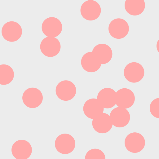
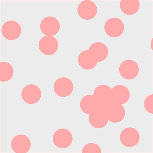
Figure 1: Initial Boolean model $\Xi\mathbbm{x}$ vs filled-up Boolean model $\boldsymbol{\boxminus}\mathbbm{x}$.

Remark 2.

We observe that

$$\Xi(\mathbbm{x}+x)=\Xi(\mathbbm{x})+x\,,\qquad\boldsymbol{\boxminus}(\mathbbm{x}+x)=\boldsymbol{\boxminus}(\mathbbm{x})+x\,.$$

As discussed in the introduction, we need to “smoothen” the geometry in order to be able to apply standard homogenization methods. Given a Lipschitz domain $P\subset\mathbb{\mathbb{R}}^{d}$, we define for $p\in\partial P$

$$\delta{\left(p\right)}:=\frac{1}{2}\sup_{\delta^{\prime}>0}\left\{\,\partial P\text{ is }\text{Lipschitz-graph in }\mathbb{B}_{\delta^{\prime}}{\left(p\right)}\right\}\,,$$

and because $\delta:\,\partial P\to\mathbb{R}_{\geq 0}$ is continuous [Hei21], we can define for bounded $P$

$$\delta(P):=\min_{p\in\partial P}\delta(p)\,.$$

Definition 3 (Thinning maps $\mathtt{F}_{n}$(see Figure 2)).

Let $\mathbbm{x}\in\mathcal{S}(\mathbb{R}^{d})$ be a point cloud. We denote the cluster of $x$ in $\mathbbm{x}$ by

$$\mathcal{C}_{\mathbbm{x}}(x):=\{y\in\mathbbm{x}\,|\,\exists\text{path from }x\text{ to }y\text{ inside }\Xi\mathbbm{x}\}.$$

We set

$$\mathtt{F}_{1,n}\mathbbm{x} :=\left\{x\in\mathbbm{x}\,|\,\forall y\in\mathbbm{x}:\,d(x,y)\notin\big{(}0,\frac{1}{n}\big{)}\cup\big{(}2r-\frac{1}{n},\,2r+\frac{1}{n}\big{)}\right\}$$

$$\mathtt{F}_{2,n}\mathbbm{x} :=\left\{x\in\mathbbm{x}\,|\,\#\mathcal{C}_{\mathbbm{x}}(x)\leq n,\,\delta{\left(\mathbb{B}_{r}{\left(\mathcal{C}_{\mathbbm{x}}(x)\right)}\right)}\geq\frac{1}{n}\right\}$$

and define the thinning map $\mathtt{F}_{n}$

$$\mathtt{F}_{n}:\ \mathcal{S}(\mathbb{R}^{d})\to\mathcal{S}(\mathbb{R}^{d})\,,\qquad\mathbbm{x}^{(n)}:=\mathtt{F}_{n}\mathbbm{x}:=\big{(}\mathtt{F}_{2,n}\circ\mathtt{F}_{1,n}\big{)}\mathbbm{x}\,.$$

$\mathtt{F}_{n}$ can be understood as a generalization of the classical Matérn construction [Mat86, SKM87]. For an arbitrary $\mathbbm{x}\in\mathcal{S}(\mathbb{R}^{d})$, we have that $(\boldsymbol{\boxminus}\mathbbm{x}^{(n)})^{\complement}$ is always minimally smooth (see 17). Furthermore, if $\mathbb{X}$ is a stationary point process (as defined later), then the same holds for $\mathbb{X}^{(n)}=\mathtt{F}_{n}\mathbb{X}$. We note that $\mathtt{F}_{n}$ is in general not monotone in $n$, i.e. $\mathtt{F}_{m}\mathbbm{x}\not\subset\mathtt{F}_{n}\mathbbm{x}$ for $m\leq n$.

            

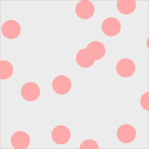
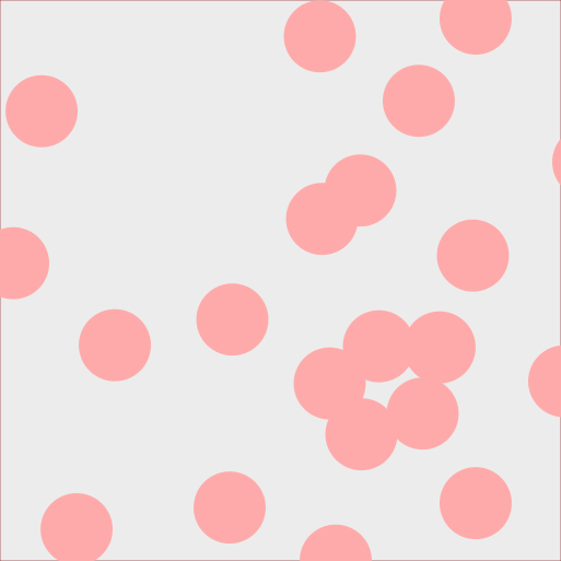
Figure 2: Thinning of point clouds under $\mathtt{F}_{n}$ pictured via the Boolean model $\Xi$. From left to right are $\mathbbm{x}$, $\mathbbm{x}^{(2)}$ and $\mathbbm{x}^{(5)}$.

Given a scale $\varepsilon>0$, we define the perforation domain $Q^{\varepsilon}$ such that the perforations have some minimal distance from the boundary $\partial Q$:

Definition 4 (Perforation of domain $Q^{\varepsilon}$).

Let $\mathbbm{x}\in\mathcal{S}(\mathbb{\mathbb{R}}^{d})$. We set

$$J^{\varepsilon}(\mathbbm{x},Q) :=\left\{x\in\mathbbm{x}\,|\,\mathrm{dist}{\left(\varepsilon\,\mathcal{C}_{\mathbbm{x}}(x)\,,\,Q^{\complement}\right)}>2\varepsilon r\right\},\qquad G_{\mathbbm{x}}^{\varepsilon}:=\varepsilon\boldsymbol{\boxminus}(J^{\varepsilon}(\mathbbm{x},Q))$$

as well as the perforated domain

$$Q_{\mathbbm{x}}^{\varepsilon}:=Q\,\backslash\,G_{\mathbbm{x}}^{\varepsilon}\,.$$

One quickly verifies that $Q_{\mathbbm{x}^{(n)}}^{\varepsilon}$ is minimally smooth (17), see 19.

1.2 Homogenization for minimally smooth perforations

We make the following parameter assumptions on our partial differential equation (LABEL:Eq:System-in-Eps).

Assumption 5 (Parameters of PDE).

Let $I=[0,T]\subset\mathbb{R}$ and $Q\subset\mathbb{R}^{d}$ be a bounded, connected open domain. We assume that

• $u_{0}\in W^{1,2}(Q)$

• $f\in L^{2}(I;L^{2}(Q))$

• $h:\ \mathbb{R}\to\mathbb{R}$ is Lipschitz continuous with Lipschitz constant $L_{h}$

• $A:\ \mathbb{R}\to\mathbb{R}$ is continuous with $0<\inf(A)$ and $\sup(A)<\infty$.

Generalized time derivatives will always be considered under the evolution triple $W^{1,2}(Q)\hookrightarrow L^{2}(Q)\hookrightarrow W^{1,2}(Q)^{*}$ or $W^{1,2}(Q_{\mathbbm{x}^{(n)}}^{\varepsilon})\hookrightarrow L^{2}(Q_{\mathbbm{x}^{(n)}}^{\varepsilon})\hookrightarrow W^{1,2}(Q_{\mathbbm{x}^{(n)}}^{\varepsilon})^{*}$ in the case of a perforated domain $Q_{\mathbbm{x}^{(n)}}^{\varepsilon}$.

Lemma 6 (Solution to PDE for minimally smooth holes).

Let $\mathbbm{x}\in\mathcal{S}(\mathbb{R}^{d})$ and $n\in\mathbb{N}$. Under 5,we have on $Q_{\mathbbm{x}^{(n)}}^{\varepsilon}$:
There exists a weak solution $u^{\varepsilon}\in L^{2}(I;W^{1,2}(Q_{\mathbbm{x}^{(n)}}^{\varepsilon}))$ with generalized time derivative $\partial_{t}u^{\varepsilon}\in L^{2}(I;W^{1,2}(Q_{\mathbbm{x}^{(n)}}^{\varepsilon})^{*})$ to LABEL:Eq:System-in-Eps.
This $u^{\varepsilon}$ satisfies for some $C>0$ depending only on $Q$, $n$, $f$ and $u_{0}$ but not on $\varepsilon$

$$\operatorname*{ess\,sup}_{t\in I}\big{\|}u^{\varepsilon}(t)\big{\|}_{L^{2}(Q_{\mathbbm{x}^{(n)}}^{\varepsilon})}+\big{\|}u^{\varepsilon}\big{\|}_{L^{2}(I;W^{1,2}(Q_{\mathbbm{x}^{(n)}}^{\varepsilon}))} \leq C$$

$$\big{\|}\partial_{t}u^{\varepsilon}\big{\|}_{L^{2}(I;W^{1,2}(Q_{\mathbbm{x}^{(n)}}^{\varepsilon})^{*})} \leq C\,.$$

The proof is given in Section 4 (47).

The next step is passing to the limit $\varepsilon\to 0$. We do so in the case that $\mathbbm{x}$ is the realization of a stationary ergodic point process $\mathbb{X}$ as defined below:

Definition 7 (Random measure and shift-operator $\tau_{x}$).

A random measure $\mu_{\bullet}$ is a random variable with values in $\mathcal{M}(\mathbb{R}^{d})$. It induces a probability distribution $\mathbb{P}$ on $\mathcal{M}(\mathbb{\mathbb{R}}^{d})$. Given the continuous map

$$\tau_{x}:\,\mathcal{M}(\mathbb{\mathbb{R}}^{d})\to\mathcal{M}(\mathbb{\mathbb{R}}^{d})\,,\qquad\tau_{x}\xi(A):=\xi(A+x)\,,$$ (3)

a random measure is stationary iff $\mathbb{P}(F)=\mathbb{P}(\tau_{x}F)$ for every $F\in\mathcal{B}(\mathcal{M}(\mathbb{\mathbb{R}}^{d}))$ and every $x\in\mathbb{\mathbb{R}}^{d}$. In line with the above setting, a random point process $\mathbb{X}$ is a random measure with $\mathbb{P}(\mathcal{S}(\mathbb{R}^{d}))=1$ and one quickly verifies that $\mathbb{X}$ is stationary iff for every $N\in\mathbb{N}$, $x\in\mathbb{\mathbb{R}}^{d}$ and bounded open $A\subset\mathbb{\mathbb{R}}^{d}$ it holds

$$\mathbb{P}\left(\mathbbm{x}\in\mathcal{S}(\mathbb{R}^{d}):\,\mathbbm{x}{\left(A\right)}=N\right)=\mathbb{P}\left(\mathbbm{x}\in\mathcal{S}(\mathbb{R}^{d}):\,\mathbbm{x}{\left(A+x\right)}=N\right).$$

We call a stationary random measure $\mu_{\bullet}$ ergodic iff the $\sigma$-algebra of $\tau$-invariant sets is trivial under its distribution $\mathbb{P}$.

Remark 8 (Compatibility of thinning with shifts).

The thinning map $\mathtt{F}_{n}$ is compatible with the shift $\tau_{x}$, i.e. on $\mathcal{S}(\mathbb{R}^{d})$

$$\mathtt{F}_{n}\circ\tau_{x}=\tau_{x}\circ\mathtt{F}_{n}\,.$$

Lemma 9 (Homogenized PDE for minimally smooth domains).

Let $\mathbb{X}$ be a stationary ergodic point process and $n\in\mathbb{N}$ fixed. For almost every realization $\mathbbm{x}$ of $\mathbb{X}$, we have under 5:
For $\varepsilon>0$, let $u^{\varepsilon}\in L^{2}(I;W^{1,2}(Q_{\mathbbm{x}^{(n)}}^{\varepsilon}))$ be a solution to LABEL:Eq:System-in-Eps. For a subsequence, there exist $\tilde{u}^{\varepsilon}\in L^{2}(I;W^{1,2}(Q))$ with $\tilde{u}^{\varepsilon}|_{Q_{\mathbbm{x}^{(n)}}^{\varepsilon}}=u^{\varepsilon}$ such that $\tilde{u}^{\varepsilon}\to u_{n}$ strongly in $L^{2}(I;L^{2}(Q))$ for some $u_{n}\in L^{2}(I;W^{1,2}(Q))$ with generalized time derivative $\partial_{t}u_{n}\in L^{2}(I;W^{1,2}(Q)^{*})$.
This $u_{n}$ is a weak solution to

$$C_{1,\mathbb{P}^{(n)}}\partial_{t}u_{n}-\nabla\cdot\big{(}A(u_{n})\mathcal{A}^{(n)}\nabla u_{n}\big{)}-C_{2,\mathbb{P}^{(n)}}h(u_{n}) =C_{1,\mathbb{P}^{(n)}}f \text{in }I\times Q$$

$$A(u_{n})\mathcal{A}^{(n)}\nabla u_{n}\cdot\nu =0 \text{on }I\times\partial Q$$ (4)

$$u_{n}(0,x) =C_{1,\mathbb{P}^{(n)}}u_{0}(x) \text{in }Q$$

with constants $C_{i,\mathbb{P}^{(n)}}>0$ depending on the distribution $\mathbb{P}^{(n)}$ of $\mathbb{X}^{(n)}$ and $\mathcal{A}^{(n)}$ being a symmetric positive semi-definite matrix – the so called effective conductivity based on the event that the origin is not covered by $\boldsymbol{\boxminus}\mathbb{X}^{(n)}$ (see 31).

This is shown in Section 4 (49) using two-scale convergence.

1.3 Homogenization for irregular perforations

When it comes to the final homogenization result, we will need the following assumptions on the point process $\mathbb{X}$.

Definition 10 (Admissible point process).

We call a point cloud $\mathbbm{x}\in\mathcal{S}(\mathbb{R}^{d})$ admissible iff the following holds (with $r>0$ from 1):

1. Equidistance Property: $\forall x,y\in\mathbbm{x}:\,\left|x-y\right|\neq 2r$.

2. Finite Clusters: For every $x\in\mathbbm{x}$, we have that $\#\mathcal{C}_{\mathbbm{x}}(x)<\infty$.

A stationary ergodic boundedly finite point process $\mathbb{X}$ is called admissible if its realizations are almost surely admissible.

Definition 11 (Statistical connectedness).

The random set $\boldsymbol{\boxminus}\mathbb{X}^{\complement}$ is statistically connected iff the effective conductivity $\mathcal{A}$ (31) based on the event that the origin is covered by $\boldsymbol{\boxminus}\mathbb{X}^{\complement}$ is strictly positive definite.

Remark 12 (Sufficient condition for statistical connectedness).

A criterion for statistical connectedness is given in Section 6, namely the existence of sufficiently many so called percolation channels. It also turns out that $\boldsymbol{\boxminus}\mathbb{X}^{\complement}$ is statistically connected if and only if the same holds for $\Xi\mathbb{X}^{\complement}$.

We may now state the main theorem of this work.

Theorem 13 (Homogenized limit for admissible point processes).

Let $\mathbb{X}$ be an admissible point process and $\boldsymbol{\boxminus}\mathbb{X}{}^{\complement}$ statistically connected. Under 5, we have for almost every realization $\mathbbm{x}$ of $\mathbb{X}$:
For every $n\in\mathbb{N}$, let $u_{n}$ be a homogenized limit from 9. Then, there exists a $u\in L^{2}(I;W^{1,2}(Q))$ with generalized time-derivative $\partial_{t}u\in L^{2}(I;W^{1,2}(Q)^{*})$ such that for a subsequence

$$u_{n} \xrightharpoonup[n\to\infty]{L^{2}(I;W^{1,2}(Q))}u\qquad\text{and}\qquad\partial_{t}u_{n}\xrightharpoonup[n\to\infty]{L^{2}(I;W^{1,2}(Q)^{*})}\partial_{t}u$$

and $u$ is a weak solution to

$$C_{1,\mathbb{P}}\partial_{t}u-\nabla\cdot\big{(}A(u)\mathcal{A}\nabla u\big{)}-C_{2,\mathbb{P}}h(u) =C_{1,\mathbb{P}}f \text{in }I\times Q$$

$$A(u)\mathcal{A}\nabla u\cdot\nu =0 \text{on }I\times\partial Q$$

$$u(0,x) =C_{1,\mathbb{P}}u_{0}(x) \text{in }Q$$

with constants $C_{i,\mathbb{P}}>0$ only depending on the distribution $\mathbb{P}$ of $\mathbb{X}$ and $\mathcal{A}$ being a symmetric positive definite matrix – the so called effective conductivity $\mathcal{A}$ based on the event that the origin is not covered by $\boldsymbol{\boxminus}\mathbb{X}$ (31). In particular, the system does not depend on the chosen thinning procedure.

Proof.

This main theorem is proven in 50. ∎

Remark 14 (Random radii).

Out of convenience, we have chosen the Boolean model with fixed radius $r$ as our underlying model. One can easily generalize the procedure to random independent radii $r\leq r_{\max}$.

Remark 15 (Homogenization procedure).

For fixed $\varepsilon>0$, solutions $u^{\varepsilon}=u_{\mathbbm{x}}^{\varepsilon}$ to LABEL:Eq:System-in-Eps exist for admissible $\mathbbm{x}\in\mathcal{S}(\mathbb{R}^{d})$ as $Q_{\mathbbm{x}^{(n)}}^{\varepsilon}=Q_{\mathbbm{x}}^{\varepsilon}$ for $n$ large enough (23). If $\mathbbm{x}$ is a realization of some admissible point process $\mathbb{X}$, then this is still not sufficient to pass to the limit $\varepsilon\to 0$. The missing regularity of $\boldsymbol{\boxminus}\mathbb{X}$ still prevents us from establishing a priori estimates.
All in all, our procedure yields the following diagram:

Statistical connectedness of $\boldsymbol{\boxminus}\mathbb{X}{}^{\complement}$ is crucial to establish $W^{1,2}(Q)$-estimates for $u_{n}$. This indicates that the direct limit passing $u^{\varepsilon}\to u$ might only rely on the statistical connectedness, but we cannot answer that as of yet.

1.4 Example: Poisson point processes

In order to demonstrate that the class of point process satisfying our assumptions is not empty, we show in Section 7 that the Poisson point process $\mathbb{X}_{\mathrm{poi}}$ is indeed suitable for our framework. We obtain the following.

Theorem 16 (Admissibility and statistical connectedness for $\mathbb{X}_{\mathrm{poi}}$).

In the subcritical regime (see 56), we have for the Poisson point process $\mathbb{X}_{\mathrm{poi}}$ that

• $\mathbb{X}_{\mathrm{poi}}$ is an admissible point process.

• $\boldsymbol{\boxminus}\mathbb{X}_{\mathrm{poi}}^{\complement}$ is statistically connected.

While admissibility is easily proven, the statistical connectedness is much harder to deal with. Most of Section 7 is dedicated to this proof. It also builds up on Section 6 in which we show that so called percolation channels yield statistical connectedness.

2 Thinning properties, surface measure and convergence of intensities

We first establish some properties of $\mathtt{F}_{n}:\ \mathcal{S}(\mathbb{R}^{d})\to\mathcal{S}(\mathbb{R}^{d})$, most importantly the minimal smoothness of $\boldsymbol{\boxminus}\mathbbm{x}^{(n)}$.

Definition 17 (Minimal smoothness [Ste16]).

An open set $P\subset\mathbb{R}^{d}$ is called minimally smooth with constants $(\delta,N,M)$ if we may cover $\partial P$ by a countable sequence of open sets $(U_{i})_{i}$ such that

1. $\forall x\in\mathbb{R}^{d}:\ \#\{U_{i}\,|\,x\in U_{i}\}\leq N$.

2. $\forall x\in\partial P\,\exists U_{i}:\ \mathbb{B}_{\delta}{\left(x\right)}\subset U_{i}$.

3. For every $i$, $\partial P\cap U_{i}$ agrees (in some Cartesian system of coordinates) with the graph of a Lipschitz function whose Lipschitz semi-norm is at most $M$.

Lemma 18 (Uniform $\delta$ on individual clusters).

Let $\mathbbm{x}\in\mathcal{S}(\mathbb{R}^{d})$ be an admissible point cloud. Then, for every $x\in\mathbbm{x}$

$$\delta{\left(\Xi{\left(\mathcal{C}_{\mathbbm{x}}(x)\right)}\right)}>0\,.$$

Proof.

Let $\mathbbm{x}\in\mathcal{S}(\mathbb{R}^{d})$ and assume $\delta{\left(\Xi{\left(\mathcal{C}_{\mathbbm{x}}(x)\right)}\right)}=0$ for some $x\in\mathbbm{x}$. Then, there must be some $p\in\partial\Xi_{\mathbbm{x}}$ with $\delta(p)=0$. This together with bounded finiteness gives $x_{p},y_{p}\in\mathbbm{x}$ such that $p\in B_{r}(x_{p})\cap B_{r}(y_{p})$, in particular $\big{|}x_{p}-y_{p}\big{|}=2r$. This contradicts the equidistance property of $\mathbbm{x}$. ∎

The thinning maps $\mathtt{F}_{n}$ have been constructed just to yield the following theorem:

Theorem 19 (Minimal smoothness of thinned point clouds).

For every $\mathbbm{x}\in\mathcal{S}(\mathbb{R}^{d})$, both $(\Xi\mathbbm{x}^{(n)})^{\complement}$ and $(\boldsymbol{\boxminus}\mathbbm{x}^{(n)})^{\complement}$ are minimally smooth with $\delta=\frac{1}{n}$, $M=\sqrt{2nr}$. Furthermore, every connected component of $\Xi\mathbbm{x}^{(n)}$ or $\boldsymbol{\boxminus}\mathbbm{x}^{(n)}$ has diameter less than $2nr$.

Proof.

It remains to verify the estimate on $M$. Let $x=o=0_{\mathbb{R}^{d}}$ and $y=\left(2r-n^{-1},0\dots,0\right)$. Then the Lipschitz constant at the intersection of the two balls $\mathbb{B}_{r}{\left(x\right)}$ and $\mathbb{B}_{r}{\left(y\right)}$ is less than $\sqrt{2nr}$. ∎

Theorem 20 (Further properties of $\mathtt{F}_{n}$).

The set $\mathcal{S}_{\mathcal{A}}(\mathbb{\mathbb{R}}^{d})$ of admissible point clouds is measurable in the vague $\sigma$-algebra. Given $n\in\mathbb{N}$, it holds that $\mathtt{F}_{n}:\,\mathcal{S}(\mathbb{\mathbb{R}}^{d})\to\mathcal{S}(\mathbb{\mathbb{R}}^{d})$ is measurable, $\mathcal{S}^{(n)}:=\mathtt{F}_{n}\mathcal{S}(\mathbb{\mathbb{R}}^{d})$ is compact in the vague topology and the following three properties of $\mathbbm{x}\in\mathcal{S}(\mathbb{\mathbb{R}}^{d})$ are equivalent:

1. $\mathtt{F}_{n}\mathbbm{x}=\mathbbm{x}$

2. $\mathbbm{x}\in\mathcal{S}^{(n)}$

3. (5)–(6) hold:

   $$\forall x,y\in\mathbbm{x},x\neq y:\quad d(x,y)\notin(0,\frac{1}{n})\cup(2r-\frac{1}{n},\,2r+\frac{1}{n})\,,$$ (5)

   $$\forall x\in\mathbbm{x}:\quad \#\mathcal{C}_{\mathbbm{x}}(x)\leq n,\,\delta{\left(\mathbb{B}_{r}{\left(\mathcal{C}_{\mathbbm{x}}(x)\right)}\right)}\geq\frac{1}{n}\,.$$ (6)

Proof.

$\mathtt{F}_{n}\mathbbm{x}=\mathbbm{x}$ implies $\mathbbm{x}\in\mathcal{S}^{(n)}$ since $\mathtt{F}_{n}\mathbbm{x}\in\mathcal{S}^{(n)}$ and vice versa $\mathbbm{x}\in\mathcal{S}^{(n)}$ implies $\mathtt{F}_{n}\mathbbm{x}=\mathbbm{x}$ by definition of $\mathtt{F}_{n}$. By construction of $\mathtt{F}_{n}$ it follows that (5)–(6) hold if and only if $\mathbbm{x}\in\mathcal{S}^{(n)}$.

Consider the space of (non-simple) counting measures $\mathcal{N}(\mathbb{R}^{d})\subset\mathcal{M}(\mathbb{R}^{d})$, i.e.

$$\mathcal{N}(\mathbb{R}^{d}):=\big{\{}\mu\in\mathcal{M}(\mathbb{R}^{d})\,|\,\text{$\mu=\sum_{k\in\mathcal{I}\subset\mathbb{N}}a_{k}\delta_{x_{k}}\text{ such that }$}a_{k}\in\mathbb{N}\text{ and }x_{k}\in\mathbb{R}^{d}\big{\}}\,.$$

We see, e.g. in [DVJ08], that

• $\mathcal{S}(\mathbb{R}^{d})$ and $\mathcal{N}(\mathbb{R}^{d})$ are both measurable w.r.t. the Borel-$\sigma$-algebra of $\mathcal{M}(\mathbb{R}^{d})$.

• $\mathcal{S}(\mathbb{R}^{d})\subset\mathcal{N}(\mathbb{R}^{d})$ and $\mathcal{N}(\mathbb{R}^{d})$ is closed in $\mathcal{M}(\mathbb{R}^{d})$. In particular, $\mathcal{N}(\mathbb{R}^{d})$ is also complete under the Prohorov metric.

Now $\mathcal{S}^{(n)}$ is precompact because of the characterization of precompact sets in the vague topology: For every bounded open $A\subset\mathbb{\mathbb{R}}^{d}$, it holds that $\sup_{\mathbbm{x}\in\mathcal{S}^{(n)}}\mathbbm{x}(A)\leq C\left(\mathrm{diam}\,A\right)^{d}$ with $C$ depending only on $n$. It remains to show that $\mathcal{S}^{(n)}$ is closed as a subset of $\mathcal{N}(\mathbb{R}^{d})$. Let $\left(\mathbbm{x}_{j}\right)_{j\in\mathbb{N}}\subset\mathcal{S}^{(n)}$ be a converging sequence with limit $\mathbbm{x}\in\mathcal{N}(\mathbb{\mathbb{R}}^{d})$. One checks that LABEL:Eq:thm:Fn-compact-and-nice-1 (namely $d(x,y)\notin\big{(}0,\frac{1}{n}\big{)}$) ensures $\mathbbm{x}\in\mathcal{S}(\mathbb{R}^{d})$, e.g. in a procedure similar to the proof of [DVJ08, Lemma 9.1.V]. We observe that for every $x,y\in\mathbbm{x}$, there exist $x_{j},y_{j}\in\mathbbm{x}_{j}$ such that $x_{j}\to x$, $y_{j}\to y$ as $j\to\infty$. This implies by a limit in (5) that $\mathbbm{x}$ still satisfies (5).

For $x\in\mathbbm{x}$, one checks that LABEL:Eq:thm:Fn-compact-and-nice-1 (namely $d(x,y)\notin\big{(}2r-\frac{1}{n},2r+\frac{1}{n}\big{)}$) implies $\#\mathcal{C}_{\mathbbm{x}}(x)\leq n$.

Let $p\in\partial\Xi(\mathbbm{x})$ and let $\left\{x^{(1)},\dots x^{(K)}\right\}=\mathbb{B}_{10r}{\left(p\right)}\cap\mathbbm{x}$ with sequences $x_{j}^{(k)}\to x^{(k)}$, $x_{j}^{(k)}\in\mathbbm{x}_{j}$. Given $\eta>0$, let $J\in\mathbb{N}$ such that for all $j>J$ and $k=1,\dots K$ it holds $\left|x^{(k)}-x_{j}^{(k)}\right|<\eta$. Then there exists $p_{j}\in\partial\Xi(\mathbbm{x}_{j})$ such that $\left|p_{j}-p\right|<\eta$ and $\partial\Xi(\mathbbm{x}_{j})$ is a Lipschitz graph in the ball $\mathbb{B}_{2\delta}{\left(p_{j}\right)}$ for every $\delta<\frac{1}{n}$. Hence $\partial\Xi(\mathbbm{x}_{j})$ is a Lipschitz graph in the ball $\mathbb{B}_{2\delta-\eta}{\left(p\right)}$. Because the Lipschitz regularity of $\partial\Xi(\mathbbm{x}_{j})$ changes continuously under slight shifts of the balls, there exists $\eta_{0}$ such that for $\eta<\eta_{0}$ and $\partial\Xi(\mathbbm{x})$ is Lipschitz graph in $\mathbb{B}_{2\delta-2\eta}{\left(p\right)}$. Since $\eta$ is arbitrary, we find $\partial\Xi(\mathbbm{x})$ is Lipschitz graph in $\mathbb{B}_{2\delta}{\left(p\right)}$ for every $\delta<n^{-1}$, implying $\delta(p)\geq\frac{1}{n}$. Since this holds for every $p$, we conclude (6) and $\mathcal{S}^{(n)}$ is compact.

To see that $\mathcal{S}_{\mathcal{A}}(\mathbb{\mathbb{R}}^{d})$ is measurable, consider for $\mathbbm{x}\in\mathcal{S}(\mathbb{\mathbb{R}}^{d})$

$$\mathbbm{x}_{1,m,R} :=\left\{x\in\mathbbm{x}\,|\,x\notin\mathbb{B}_{R}{\left(o\right)}\text{ or }\,d(x,y)\notin(0,\frac{1}{m})\cup(2r-\frac{1}{m},\,2r+\frac{1}{m})\ \forall y\in\mathbbm{x}\right\}\,,$$

$$\mathbbm{x}_{2,l,R} :=\left\{x\in\mathbbm{x}\,|\,x\notin\overline{\mathbb{B}_{R}{\left(o\right)}}\text{ or }\#\mathcal{C}_{\mathbbm{x}}(x)\leq l,\,\delta{\left(\mathbb{B}_{r}{\left(\mathcal{C}_{\mathbbm{x}}(x)\right)}\right)}>\frac{1}{l}\right\}\,,$$

and define

$$\mathtt{F}_{1,m,R}\mathbbm{x} :=\mathbbm{x}_{1,m,R} \mathcal{S}^{(1,m,R)} :=\mathtt{F}_{1,m,R}\mathcal{S}(\mathbb{R}^{d})$$

$$\mathtt{F}_{2,l,R}\mathbbm{x} :=\mathbbm{x}_{2,l,R}\,. \mathcal{S}^{(2,m,R)} :=\mathtt{F}_{2,m,R}\mathcal{S}(\mathbb{R}^{d})\,.$$

We check that $\mathcal{S}^{(1,m,R)}$ is a closed subset inside $\mathcal{S}(\mathbb{R}^{d})$ (repeat the arguments above), i.e. $\overline{\mathcal{S}^{(1,m,R)}}\cap\mathcal{S}(\mathbb{R}^{d})=\mathcal{S}^{(1,m,R)}$. In particular, $\mathcal{S}^{(1,m,R)}$ is measurable w.r.t. the vague topology of $\mathcal{M}(\mathbb{R}^{d})$. Similarly, one shows that $\mathcal{S}(\mathbb{R}^{d})\backslash\mathcal{S}^{(2,m,R)}$ is closed as a subset inside $\mathcal{S}(\mathbb{R}^{d})$. Again, this shows that $\mathcal{S}^{(2,m,R)}$ is measurable. Consider now the measurable sets

$$\mathcal{S}^{(1,\infty,\infty)}:=\bigcap_{R\in\mathbb{N}}\bigcup_{m\in\mathbb{N}}\mathcal{S}^{(1,m,R)}\qquad\text{and}\qquad\mathcal{S}^{(2,\infty,\infty)}:=\bigcap_{R\in\mathbb{N}}\bigcup_{m\in\mathbb{N}}\mathcal{S}^{(2,m,R)}\,.$$

We see that

1. $\mathbbm{x}\in\mathcal{S}^{(1,\infty,\infty)}$ if and only if for all $x,y\in\mathbbm{x}$ , it holds $d(x,y)\neq r$.

2. $\mathbbm{x}\in\mathcal{S}^{(2,\infty,\infty)}$ if and only if for every $x\in\mathbbm{x}$, it holds that $\#\mathcal{C}_{\mathbbm{x}}(x)<\infty$ and $\delta{\left(\mathbb{B}_{r}{\left(\mathcal{C}_{\mathbbm{x}}(x)\right)}\right)}>0$.

Therefore,

$$\mathcal{S}_{\mathcal{A}}(\mathbb{\mathbb{R}}^{d})=\mathcal{S}^{(1,\infty,\infty)}\cap\mathcal{S}^{(2,\infty,\infty)}$$

is measurable.

To see that $\mathtt{F}_{n}:\ \mathcal{S}(\mathbb{\mathbb{R}}^{d})\to\mathcal{S}(\mathbb{\mathbb{R}}^{d})$ is measurable, recall $\mathtt{F}_{n}=\mathtt{F}_{2,n}\circ\mathtt{F}_{1,n}$ from 3. It therefore suffices to show that the following maps are measurable:

$$\mathtt{F}_{1,n}:\ \mathcal{S}(\mathbb{R}^{d})\to\mathtt{F}_{1,n}\mathcal{S}(\mathbb{R}^{d})\subset\mathcal{S}(\mathbb{R}^{d})\qquad\text{and}\qquad\mathtt{F}_{2,n}:\ \mathtt{F}_{1,n}\mathcal{S}(\mathbb{R}^{d})\to\mathcal{S}(\mathbb{R}^{d})\,.$$

For $f\in C_{c}(\mathbb{\mathbb{R}}^{d})$, consider the evaluation by $f$, i.e.

$$M_{f}:\,\mathcal{S}(\mathbb{\mathbb{R}}^{d})\to\mathbb{R}\,,\qquad\mathbbm{x}\mapsto\int_{\mathbb{\mathbb{R}}^{d}}f\,\mathrm{d}\mathbbm{x}\,.$$

If $f\geq 0$, we observe the upper semi-continuity of

$$M_{f}\circ\mathtt{F}_{1,n}:\ \mathcal{S}(\mathbb{R}^{d})\to\mathbb{R}\qquad\text{and}\qquad M_{f}\circ\mathtt{F}_{2,n}:\ \mathtt{F}_{1,n}\mathcal{S}(\mathbb{R}^{d})\to\mathbb{R}\,.$$

We have lower semi continuity for $f\leq 0$ since $M_{-f}=-M_{f}$. Therefore $M_{f}\circ\mathtt{F}_{i,n}$ with $i\in\{1,2\}$ is measurable in the cases $f\geq 0$ and $f\leq 0$ and hence in general. Since the vague topology is generated by $\big{(}M_{f}\big{)}_{f\in C_{c}(\mathbb{R}^{d})}$, we conclude that $\mathtt{F}_{1,n}$ and $\mathtt{F}_{2,n}$ are measurable. ∎

Remark 21 (Fine details of 20).

• For $\mathcal{S}^{(n)}:=\mathtt{F}_{n}(\mathcal{S}(\mathbb{R}^{d})$), we have that

  $$\bigcup_{n\in\mathbb{N}}\mathcal{S}^{(n)}\subsetneq\mathcal{S}_{\mathcal{A}}(\mathbb{R}^{d})\subsetneq\big{\{}\mathbbm{x}\,|\,\lim_{n\to\infty}\mathtt{F}_{n}\mathbbm{x}=\mathbbm{x}\big{\}}\subsetneq\mathcal{S}(\mathbb{R}^{d})\subsetneq\overline{\bigcup_{n\in\mathbb{N}}\mathcal{S}^{(n)}}=\mathcal{N}(\mathbb{R}^{d})\,.$$

• $M_{f}\circ\mathtt{F}_{2,n}$ is not upper semi-continuous on $\mathcal{S}(\mathbb{R}^{d})$ (in contrast to $\mathtt{F}_{1,n}\mathcal{S}(\mathbb{R}^{d})$): The condition that $d(x,y)\notin(2r-\frac{1}{n},\,2r+\frac{1}{n})\ \forall x,y\in\mathtt{F}_{1,n}\mathbbm{x}$ is crucial to ensure that clusters do not change sizes.

Definition 22.

We define the events that the origin is not covered by the filled-up Boolean model, i.e.

$$\mathbf{G}:=\left\{\mathbbm{x}\in\mathcal{S}(\mathbb{R}^{d})\,|\,o\notin\boldsymbol{\boxminus}\mathbbm{x}\right\}\qquad\text{and}\qquad\mathbf{G}_{n}:=\mathtt{F}_{n}{}^{-1}(\mathbf{G})=\left\{\mathbbm{x}\in\mathcal{S}(\mathbb{R}^{d})\,|\,o\notin\boldsymbol{\boxminus}\mathbbm{x}^{(n)}\right\}\,.$$

This gives us for $x\in\mathbb{R}^{d}$ that

$$\mathds{1}_{\boldsymbol{\boxminus}\mathbbm{x}^{\complement}}(x)=\mathds{1}_{\mathbf{G}}(\tau_{x}\mathbbm{x})\,.$$

We will later consider the effective conductivities based on these events.

Theorem 23 (Approximation properties).

Let $\mathbbm{x}\in\mathcal{S}(\mathbb{R}^{d})$ be an admissible point cloud.

1. For every bounded domain $\Lambda$, there exists an $N(\mathbbm{x},\Lambda)\in\mathbb{N}$ such that for every $n\geq N(\mathbbm{x},\Lambda)$

   $$\mathbbm{x}^{(n)}\cap\Lambda=\mathbbm{x}\cap\Lambda\,,\qquad\text{in particular}\qquad\mathbbm{x}=\bigcup_{n\in\mathbb{N}}\mathbbm{x}^{(n)}\,.$$

2. For every bounded domain $\Lambda$, there exists an $\tilde{N}(\mathbbm{x},\Lambda)\in\mathbb{N}$ such that for every $n\geq\tilde{N}(\mathbbm{x},\Lambda)$

   $$\boldsymbol{\boxminus}\mathbbm{x}{}^{(n)}\cap\Lambda=\boldsymbol{\boxminus}\mathbbm{x}\cap\Lambda,\qquad\text{in particular}\qquad\boldsymbol{\boxminus}\mathbbm{x}=\bigcup_{n\in\mathbb{N}}\boldsymbol{\boxminus}\mathbbm{x}{}^{(n)}.$$

3. There exists an $N=N(\mathbbm{x})\in\mathbb{N}$ such that for every $n\geq N$:

   $$o\notin\boldsymbol{\boxminus}\mathbbm{x}^{(n)}\iff o\notin\boldsymbol{\boxminus}\mathbbm{x}\,.$$

   In particular, $\bigcap_{n\in\mathbb{N}}\mathbf{G}_{n}\backslash\mathbf{G}$ only consists of non-admissible point clouds.

Proof.

1. Boundedness of $\Lambda$ implies that there are only finitely many mutually disjoint clusters $\mathcal{C}_{\mathbbm{x}}(x_{i})$, $i=1,\dots,N_{\mathcal{C}}$ that intersect with $\Lambda$. Furthermore, because $\#\left(\mathbbm{x}\cap\mathbb{B}_{r}{\left(\Lambda\right)}\right)<\infty$ and because of Property 1 of admissible point clouds, we know

   $$\min\left\{\left|\left|x-y\right|-2r\right|:\,x,y\in\mathbbm{x}\cap\mathbb{B}_{r}{\left(\Lambda\right)},\,x\neq y\right\}>0$$

   and 18 yields

   $$\min\left\{\delta{\left(\Xi\mathcal{C}_{\mathbbm{x}}(x_{i})\right)}:\,\mathcal{C}_{\mathbbm{x}}(x_{i})\cap\Lambda\neq\emptyset\right\}>0\,.$$

   This implies the first statement.

2. By making $\Lambda$ larger, we may assume $\Lambda=[-k,k]^{d}$ for some $k\in\mathbb{N}$. For $n\geq N(\mathbb{B}_{r}{\left([-k,k]^{d}\right)})$:

   $$[-k,k]^{d}\backslash\Xi\mathbbm{x}^{(n)}=[-k,k]^{d}\backslash\Xi\mathbbm{x}.$$

   $[-k,k]^{d}\backslash\Xi\mathbbm{x}$ only has finitely many connected components $\mathcal{C}_{i}$. Take one of these connected components $\mathcal{C}_{i}$ and suppose it lies in $\boldsymbol{\boxminus}\mathbbm{x}$. Then, it has to be encircled by finitely many balls $\mathbb{B}_{r}{\left(x\right)}$ in $\Xi\mathbbm{x}$. Let $n_{i}$ large enough such that all these $x$ lie in $\mathbbm{x}^{(n_{i})}$. Then, $\mathcal{C}_{i}\subset\boldsymbol{\boxminus}\mathbbm{x}^{(n_{i})}$. We may do so for every $\mathcal{C}_{i}$. Take

   $$\tilde{N}(\mathbbm{x},\Lambda):=\max\big{\{}n_{i},\,N(\mathbb{B}_{r}{\left([-k,k]^{d}\right)})\big{\}}.$$

   For every $n\geq\tilde{N}(\mathbbm{x},\Lambda)$, the connected components $\mathcal{C}_{i}$ of $[-k,k]^{d}\backslash\Xi\mathbbm{x}^{(n)}$ and $[-k,k]^{d}\backslash\Xi\mathbbm{x}$ are identical since $[-k,k]^{d}\backslash\Xi\mathbbm{x}^{(n)}=[-k,k]^{d}\backslash\Xi\mathbbm{x}$. Therefore, we get the claim

   $$[-k,k]^{d}\backslash\boldsymbol{\boxminus}\mathbbm{x}^{(n)} =\Big{(}[-k,k]^{d}\backslash\Xi\mathbbm{x}^{(n)}\Big{)}\backslash\bigcup_{C_{i}\subset\boldsymbol{\boxminus}\mathbbm{x}^{(n)}}\mathcal{C}_{i}$$

   $$=\Big{(}[-k,k]^{d}\backslash\Xi\mathbbm{x}\Big{)}\backslash\bigcup_{C_{i}\subset\boldsymbol{\boxminus}\mathbbm{x}}\mathcal{C}_{i}\quad=[-k,k]^{d}\backslash\boldsymbol{\boxminus}\mathbbm{x}\,.$$

3. This is a direct consequence of Point 2. If $\mathbbm{x}\in\bigcap_{n\in\mathbb{N}}\mathbf{G}_{n}\backslash\mathbf{G}$, then $o\notin\boldsymbol{\boxminus}\mathbbm{x}^{(n)}$ for every $n$ but $o\in\boldsymbol{\boxminus}\mathbbm{x}$. Therefore, $\mathbbm{x}$ cannot be admissible by Point 2.

∎

Definition 24 (Surface measure of $\boldsymbol{\boxminus}\mathbbm{x}$).

We define the surface measure for $\mathbbm{x}\in\mathcal{S}(\mathbb{R}^{d})$

$$\mu_{\mathbbm{x}}(A):=\mathcal{H}_{\llcorner\partial\boldsymbol{\boxminus}\mathbbm{x}}^{d-1}(A)=\mathcal{H}^{d-1}(A\cap\partial\boldsymbol{\boxminus}\mathbbm{x})\,.$$

Note that $\mu_{\mathbbm{x}}{\left([0,1]^{d}\right)}\leq\mathcal{H}^{d-1}{\left(\mathbb{B}_{r}{\left(o\right)}\right)}\,\cdot\,\mathbbm{x}{\left(\mathbb{B}_{r}{\left([0,1]^{d}\right)}\right)}$.

Remark 25 (Distributions of $\mathbb{X}^{(n)},\,\mu_{\bullet}$).

Given a point process $\mathbb{X}$, we can consider $\mathbb{X}^{(n)}$ and $\mu_{\mathbb{X}}$. Both come with their own distributions, but they are still driven by $\mathbb{X}$ in a $\tau$-compatible way. Therefore, we can express their distributions and all relevant quantities in terms of the distribution $\mathbb{P}$ of $\mathbb{X}$. For example, the distribution of $\mathbb{X}^{(n)}$ is $\mathbb{P}\circ\mathtt{F}_{n}{}^{-1}$.

Definition 26 (Intensity of random measure).

Given a stationary random measure $\tilde{\mu}$, we define its intensity to be

$$\lambda(\tilde{\mu}):=\mathbb{E}\big{[}\tilde{\mu}\big{(}[0,1)^{d}\big{)}\big{]}\,.$$

Lemma 27 (Convergence of intensities).

Let $\mathbb{X}$ be an admissible point process with finite intensity $\lambda(\mathbb{X})$. Then,

$$\lim_{n\to\infty}\lambda(\mathbb{X}^{(n)})=\lambda(\mathbb{X})\qquad\text{and}\qquad\lim_{n\to\infty}\lambda(\mu_{\mathbb{X}^{(n)}})=\lambda(\mu_{\mathbb{X}})\,.$$

Proof.

“Almost surely” is to be understood w.r.t. the distribution $\mathbb{P}$ of $\mathbb{X}$.

1. By 23, we have almost surely $\mathbb{X}^{(n)}{\left([0,1]^{d}\right)}\to\mathbb{X}{\left([0,1]^{d}\right)}$ as $n\to\infty$. Dominated convergence with majorant $\mathbb{X}{\left([0,1]^{d}\right)}$ yields

   $$\lambda(\mathbb{X}^{(n)})=\mathbb{E}[\mathbbm{x}^{(n)}{\left([0,1]^{d}\right)}]\to\mathbb{E}[\mathbbm{x}{\left([0,1]^{d}\right)}]=\lambda(\mathbb{X}).$$

2. Again, by 23, we have almost surely $\boldsymbol{\boxminus}\mathbb{X}^{(n)}\cap[0,1]^{d}\to\boldsymbol{\boxminus}\mathbb{X}\cap[0,1]^{d}$, in particular

   $$\mu_{\mathbb{X}^{(n)}}{\left([0,1]^{d}\right)}=\mathcal{H}_{\llcorner\partial\boldsymbol{\boxminus}\mathbb{X}^{(n)}}^{d-1}{\left([0,1]^{d}\right)}\to\mathcal{H}_{\llcorner\partial\boldsymbol{\boxminus}\mathbb{X}}^{d-1}{\left([0,1]^{d}\right)}=\mu_{\mathbb{X}}{\left([0,1]^{d}\right)}.$$

   Dominated convergence yields again convergence of intensities.

∎

Remark 28 (Local convergence).

The convergence in 23 is much stronger than what is actually needed to prove the convergence of intensities. Indeed, we could prove convergence even for so called tame and local functions $f:\ \mathcal{M}(\mathbb{R}^{d})\to\mathbb{R}$ for which the intensity $\lambda$ is just one special case $f(\mathbbm{x}):=\mathbbm{x}{\left([0,1]^{d}\right)}$.

3 Effective conductivity and cell solutions

The structure $(\mathcal{M}(\mathbb{R}^{d}),\mathcal{B}(\mathcal{M}(\mathbb{R}^{d})),\mathbb{P},\tau)$ as in 7 is a so called dynamical system:

Definition 29 (Dynamical system, stationarity, ergodicity).

Let $(\Omega,\mathcal{F},\mathcal{P})$ be a separable metric probability space. A dynamical system $\tau=(\tau_{x})_{x\in\mathbb{R}^{d}}$ is a family of measurable mappings $\tau_{x}:\ \Omega\to\Omega$ satisfying

• Group property:
  $\tau_{0}=\text{id}_{\Omega}$ and $\tau_{x+y}=\tau_{x}\circ\tau_{y}$ for any $x,\,y\in\mathbb{R}^{d}$.

• Measure preserving:
  For any $x\in\mathbb{R}^{d}$ and any $F\in\mathcal{F}$, we have $\mathcal{P}\left(\tau_{x}(F)\right)=\mathcal{P}\left(F\right)$.

• Continuity:
  The map $\mathcal{T}:\ \Omega\times\mathbb{R}^{d}\to\Omega$, $\left(\omega,\,x\right)\mapsto\tau_{x}(\omega)$ is continuous w.r.t. the product topology on $\Omega\times\mathbb{R}^{d}$.

$\tau$ is called ergodic if the $\sigma$-algebra of $\tau$-invariant sets is trivial under $\mathcal{P}$.

Our practical setting will always be some $\Omega\subset\mathcal{M}(\mathbb{R}^{d})$, but we will still work with abstract dynamical systems in Section 3 and 4.

3.1 Potentials and solenoidals

Let $(\Omega,\mathcal{B}(\Omega),\mathcal{P},\tau)$ be a dynamical system. We write $L^{2}(\Omega):=L^{2}(\Omega,\,\mathcal{P})$. The dynamical system $\tau$ introduces a strongly continuous group action on $L^{2}(\Omega)\to L^{2}(\Omega)$ through $T_{x}f(\omega):=f(\tau_{x}\omega)$ with the $d$ independent generators

$$\mathrm{D}_{i}f:=\lim_{t\to 0}\frac{1}{t}\left(f-f(\tau_{te_{i}}\bullet)\right)$$

with domain $\mathcal{D}_{i}$ where $\left(e_{i}\right)_{i=1,\dots,d}\subset\mathbb{R}^{d}$ is the canonical Euclidean basis. Introducing

$$H^{1}(\Omega):=\bigcap_{i=1}^{d}\mathcal{D}_{i}\subset L^{2}(\Omega)$$

and the gradient $\nabla_{\omega}f:=\left(\mathrm{D}_{1}f,\dots,\mathrm{D}_{d}f\right)^{\top}$, we can define the space of potential vector fields

$$\mathcal{V}_{\mathrm{pot}}^{2}(\Omega):=\big{\{}\nabla_{\tilde{\omega}}f\,|\,f\in H^{1}(\Omega)\text{ and }\int_{\Omega}\nabla_{\tilde{\omega}}f\text{\,$\mathrm{d}$}\mathcal{P}(\omega)=0_{\mathbb{R}^{d}}\big{\}}\,.$$

Defining $L_{\mathrm{sol}}^{2}(\Omega):=\mathcal{V}_{\mathrm{pot}}^{2}(\Omega)^{\bot}$, we find with $u_{\omega}(x):=u(\tau_{x}\omega)$

$$L_{\mathrm{pot}}^{2}(\Omega) :=\left\{u\in L^{2}(\Omega;\mathbb{\mathbb{R}}^{d})\,:\,u_{\omega}\in L_{\mathrm{pot},\mathrm{loc}}^{2}(\mathbb{\mathbb{R}}^{d})\,\,\mbox{for }\mathcal{P}-\mbox{a.e. }\omega\in\Omega\right\}\,,$$

$$L_{\mathrm{sol}}^{2}(\Omega) =\left\{u\in L^{2}(\Omega;\mathbb{\mathbb{R}}^{d})\,:\,u_{\omega}\in L_{\mathrm{sol},\mathrm{loc}}^{2}(\mathbb{\mathbb{R}}^{d})\,\,\mbox{for }\mathcal{P}-\mbox{a.e. }\omega\in\Omega\right\}\,,$$ (7)

$$\mathcal{V}_{\mathrm{pot}}^{2}(\Omega) =\big{\{}u\in L_{\mathrm{pot}}^{2}(\Omega)\,:\,\int_{\Omega}u\,\mathrm{d}\mathcal{P}=0\big{\}}\,,$$

because $\Omega$ is separable metric and where

$$L_{\mathrm{pot},\mathrm{loc}}^{2}(\mathbb{\mathbb{R}}^{d}) :=\left\{u\in L_{\mathrm{loc}}^{2}(\mathbb{\mathbb{R}}^{d};\mathbb{\mathbb{R}}^{d})\,\,|\,\,\forall U\,\,\mbox{bounded domain }\exists\varphi\in W^{1,2}(U)\,:\,u=\nabla\varphi\right\}\,,$$

$$L_{\mathrm{sol},\mathrm{loc}}^{2}(\mathbb{\mathbb{R}}^{d}) :=\big{\{}u\in L_{\mathrm{loc}}^{2}(\mathbb{\mathbb{R}}^{d};\mathbb{\mathbb{R}}^{d})\,\,|\,\,\int_{\mathbb{\mathbb{R}}^{d}}u\cdot\nabla\varphi=0\,\,\forall\varphi\in C_{c}^{1}(\mathbb{\mathbb{R}}^{d})\big{\}}\,.$$

For $A\subset\Omega$ measurable, we define

$$\mathcal{V}_{\mathrm{pot}}^{2}(A|\Omega):=cl_{L^{2}(A)^{d}}\left\{v_{|_{A}}\,|\,v\in\mathcal{V}_{\mathrm{pot}}^{2}(\Omega)\right\}.$$

3.2 Cell solutions and effective conductivity

Definition 30 (Cell solutions).

Let $(\Omega,\mathcal{B}(\Omega),\mathcal{P})$ be a separable metric probability space with dynamical system $\tau$ and let $\mathcal{Q}\in\mathcal{B}(\Omega)$. The $i$-th cell solution $w_{i}\in\mathcal{V}_{\mathrm{pot}}^{2}(\mathcal{Q}|\Omega)$ is the unique solution (after the Riesz representation theorem) of

$$\forall v\in\mathcal{V}_{\mathrm{pot}}^{2}(\Omega):\qquad\int_{\mathcal{Q}}[w_{i}+e_{i}]\cdot v\text{\,$\mathrm{d}$}\mathcal{P}(\omega)=0\,.$$

The cell solutions satisfy

$$\big{\|}w_{i}\big{\|}_{L^{2}(\mathcal{Q})^{d}}\leq\sqrt{\mathcal{P}(\mathcal{Q})}\leq 1\,,$$

and can be grouped in the matrix

$$W_{\mathcal{Q}}:=(w_{1},\dots,w_{d})\,.$$

Definition 31 (Effective conductivity $\mathcal{A}$).

Let $w_{i}$ the cell solution on $\mathcal{Q}\in\mathcal{B}(\Omega)$. The effective conductivity $\mathcal{A}$ based on the event $\mathcal{Q}$ is defined as

$$\mathcal{A} :=\int_{\mathcal{Q}}(I_{d}+W_{\mathcal{Q}})^{t}(I_{d}+W_{\mathcal{Q}})\text{\,$\mathrm{d}$}\mathcal{P}(\omega)\,.$$ (8)

with $I_{d}$ being the identity matrix. We observe for the entries $\left(\mathcal{A}_{i,j}\right)_{i,j=1,\dots,d}$ of $\mathcal{A}$ that

$$\mathcal{A}_{i,j} =\int_{\mathcal{Q}}\left[e_{i}+w_{i}(\omega)\right]\cdot\left[e_{j}+w_{j}(\omega)\right]\text{\,$\mathrm{d}$}\mathcal{P}(\omega)=\int_{\mathcal{Q}}\left[e_{i}+w_{i}(\omega)\right]\cdot e_{j}\text{\,$\mathrm{d}$}\mathcal{P}(\omega)\,.$$ (9)

We write $\alpha_{\mathcal{A}}\geq 0$ for its smallest eigenvalue.

Theorem 32 (Convergence of cell solutions).

Let $\left(\mathcal{Q}_{n}\right)_{n\in\mathbb{N}}\subset\mathcal{B}(\Omega)$ and $\mathcal{Q}\in\mathcal{B}(\Omega)$ such that $\mathds{1}_{\mathcal{Q}_{n}}\to\mathds{1}_{\mathcal{Q}}$ $\mathcal{P}$-almost surely and $\mathcal{Q}_{n}\supset\mathcal{Q}$ for every $n\in\mathbb{N}$. The sequence of cell solutions $w_{i}^{(n)}$ to the cell problem on $\mathcal{Q}_{n}$ satisfies

$$w_{i}^{(n)}\rightharpoonup w_{i}\qquad\text{as }n\to\infty\,,$$

where $w_{i}\in\mathcal{V}_{\mathrm{pot}}^{2}(\mathcal{Q}|\Omega)$ is the $i$-th cell solution on $\mathcal{Q}$

$$\forall v\in\mathcal{V}_{\mathrm{pot}}^{2}(\Omega):\qquad\int_{\mathcal{Q}}\left[w_{i}+e_{i}\right]\cdot v\text{\,$\mathrm{d}$}\mathcal{P}(\omega)=0\,.$$

Proof.

We first check that the limit satisfies $\int_{\mathcal{Q}}\left[w_{i}+e_{i}\right]\cdot v\text{\,$\mathrm{d}$}\mathcal{P}(\omega)=0$ and then $w_{i}\in\mathcal{V}_{\mathrm{pot}}^{2}(\mathcal{Q}|\Omega)$.

1. The a priori estimate yields a $L^{2}$-weakly convergent subsequence of $w_{i}^{(n)}\rightharpoonup w_{i}\in L^{2}(\Omega)^{d}$ after extending $w_{i}^{(n)}$ to the whole of $\Omega$ via 0. Let $v\in\mathcal{V}_{\mathrm{pot}}^{2}(\Omega)$. We have $\mathds{1}_{\mathcal{Q}_{n}}\to\mathds{1}_{\mathcal{Q}}$ $\mathcal{P}$-almost surely, so dominated convergence yields

$$\lim_{n\to\infty}\int_{\mathcal{Q}_{n}}e_{i}\cdot v\text{\,$\mathrm{d}$}\mathcal{P}(\omega) =\int_{\mathcal{Q}}e_{i}\cdot v\text{\,$\mathrm{d}$}\mathcal{P}(\omega)$$

while weak convergence yields

$$\lim_{n\to\infty}\int_{\mathcal{Q}_{n}}w_{i}^{(n)}\cdot v\text{\,$\mathrm{d}$}\mathcal{P}(\omega) =\int_{\Omega}w_{i}\cdot v\text{\,$\mathrm{d}$}\mathcal{P}(\omega)$$

We also have

$$\mathds{1}_{\mathcal{Q}_{n}}w_{i}^{(n)}=w_{i}^{(n)}\xrightharpoonup[n\to\infty]{L^{2}(\Omega)}w_{i}\,,$$

which implies

$$\mathds{1}_{\mathcal{Q}}w_{i}=w_{i}.$$

Therefore, with $w_{i}\in L^{2}(\mathcal{Q})^{d}$:

$$0 =\lim_{n\to\infty}\int_{\mathcal{Q}_{n}}[w_{i}^{(n)}+e_{i}]\cdot v\text{\,$\mathrm{d}$}\mathcal{P}(\omega)=\int_{\mathcal{Q}}\left[w_{i}+e_{i}\right]\cdot v\text{\,$\mathrm{d}$}\mathcal{P}(\omega)\,.$$

2. $\mathcal{V}_{\mathrm{pot}}^{2}(\mathcal{Q}|\Omega)\subset L^{2}(\mathcal{Q})^{d}$ is closed and convex, so it is also weakly closed. We construct a weakly converging sequence in $\mathcal{V}_{\mathrm{pot}}^{2}(\mathcal{Q}|\Omega)$ that converges to $w_{i}$. Since $w_{i}^{(n)}\in\mathcal{V}_{\mathrm{pot}}^{2}(\mathcal{Q}_{n}|\Omega)$, we find $v^{(n)}\in\mathcal{V}_{\mathrm{pot}}^{2}(\Omega)$ such that

$$\|w_{i}^{(n)}-\mathds{1}_{\mathcal{Q}_{n}}v^{(n)}\|_{L^{2}(\mathcal{Q})^{d}}\leq\frac{1}{n}\,.$$

Since $w_{i}^{(n)}\rightharpoonup w_{i}$, we get

$$\mathds{1}_{\mathcal{Q}_{n}}v^{(n)}\xrightharpoonup[n\to\infty]{L^{2}(\Omega)^{d}}w_{i}\,.$$

Note that $\left(\mathds{1}_{\mathcal{Q}_{n}}-\mathds{1}_{\mathcal{Q}}\right)v^{(n)}$ is a bounded sequence that is point-wise convergent to 0 because of the weak convergence above and $\mathcal{Q}_{n}\supseteq\mathcal{Q}$. Therefore, it is weakly convergent to 0 and we obtain

$$\mathds{1}_{\mathcal{Q}}v^{(n)}\xrightharpoonup[n\to\infty]{L^{2}(\Omega)^{d}}w_{i}\,.$$

$\mathds{1}_{\mathcal{Q}}v^{(n)}\in\mathcal{V}_{\mathrm{pot}}^{2}(\mathcal{Q}|\Omega)$, so we get that $w_{i}\in\mathcal{V}_{\mathrm{pot}}^{2}(\mathcal{Q}|\Omega)$. ∎

Corollary 33 (Convergence of effective conductivities).

Let $\left(\mathcal{Q}_{n}\right)_{n\in\mathbb{N}}\subset\mathcal{B}(\Omega)$ and $\mathcal{Q}\in\mathcal{B}(\Omega)$ such that $\mathds{1}_{\mathcal{Q}_{n}}\to\mathds{1}_{\mathcal{Q}}$ $\mathcal{P}$-almost surely and $\mathcal{Q}_{n}\supset\mathcal{Q}$ for every $n\in\mathbb{N}$. Let $\mathcal{A}^{(n)}$ be the effective conductivity of $\mathcal{Q}_{n}$ and $\mathcal{A}$ be the effective conductivity of $\mathcal{Q}$. Then,

$$\mathcal{A}^{(n)}\xrightarrow{n\to\infty}\mathcal{A}\,.$$

Proof.

This follows from LABEL:Eq:eff-cond-linear and weak convergence $w_{i}^{(n)}\rightharpoonup w_{i}$. ∎

Remark 34 (Variational formulation).

There is another way to define $\mathcal{A}$: For $\eta\in\mathbb{R}^{d}$, $W_{\mathcal{Q}}\eta$ (see 30) is the unique minimizer to

$$\min_{\varphi\in\mathcal{V}_{\mathrm{pot}}^{2}(\mathcal{Q})}\int_{\mathcal{Q}}\big{|}\eta+\varphi\big{|}^{2}\text{\,$\mathrm{d}$}\mathcal{P}(\omega)$$

and therefore

$$\eta^{t}\mathcal{A}\eta=\int_{\mathcal{Q}}\big{|}(I_{d}+W_{\mathcal{Q}})\eta\big{|}^{2}\text{\,$\mathrm{d}$}\mathcal{P}(\omega)=\min_{\varphi\in\mathcal{V}_{\mathrm{pot}}^{2}(\mathcal{Q})}\int_{\mathcal{Q}}\big{|}\eta+\varphi\big{|}^{2}\text{\,$\mathrm{d}$}\mathcal{P}(\omega).$$

This equality is related to 51.

3.3 Pull-back for thinning maps

In Section 4, we will use two-scale convergence to homogenize LABEL:Eq:System-in-Eps for fixed $n$. This process is more convenient to handle if the underlying probability space is compact. Here we show that we may take $\mathtt{F}_{n}\mathcal{S}(\mathbb{R}^{d})$ as the underlying probability space instead of $\mathcal{S}(\mathbb{R}^{d})$.

Theorem 35.

Let $\mathcal{P}$ be a distribution on $\mathcal{S}(\mathbb{\mathbb{R}}^{d})$ and let $\mathcal{S}^{(n)}:=\mathtt{F}_{n}\mathcal{S}(\mathbb{R}^{d})$ with the push-forward measure $\tilde{\mathcal{P}}_{n}:=\mathcal{P}\circ\mathtt{F}_{n}^{-1}$. Recall $\mathbf{G}_{n}:=\left\{\mathbbm{x}\in\mathcal{S}(\mathbb{R}^{d}):\,o\notin\boldsymbol{\boxminus}\mathbbm{x}^{(n)}\right\}$ and let $\tilde{\mathbf{G}}_{n}:=\left\{\mathbbm{x}\in\mathcal{S}^{(n)}:\,o\notin\boldsymbol{\boxminus}\mathbbm{x}\right\}=\mathtt{F}_{n}\mathbf{G}_{n}$. Let $w_{i}^{(n)}$ be the cell solutions on $\mathbf{G}_{n}$ and $\tilde{w}_{i}^{(n)}$ the cell solutions on $\tilde{\mathbf{G}}_{n}$ for their respective dynamical systems. Then, for every $i,j\in\left\{1,\dots,d\right\}$, it holds that

$$\int_{\mathbf{G}_{n}}\big{[}w_{i}^{(n)}+e_{i}\big{]}\cdot e_{j}\text{\,$\mathrm{d}$}\mathcal{P}=\int_{\tilde{\mathbf{G}}_{n}}\big{[}\tilde{w}_{i}^{(n)}+e_{i}\big{]}\cdot e_{j}\text{\,$\mathrm{d}$}\tilde{\mathcal{P}}_{n}\,.$$ (10)

Lemma 36 (Properties of pull-back functions).

Let $(\Omega,\mathcal{F},\mathcal{P},\tau)$, $(\tilde{\Omega},\tilde{\mathcal{F}},\tilde{\mathcal{P}},\tilde{\tau})$ be dynamical systems, $\phi:\ \Omega\to\tilde{\Omega}$ measurable such that $\tilde{\mathcal{P}}=\mathcal{P}\circ\phi^{-1}$ and such that for every $x\in\mathbb{R}^{d}$

$$\phi\circ\tau_{x}=\tilde{\tau}_{x}\circ\phi\,.$$ (11)

Then, the following holds:
For every $\tilde{f}\in L^{2}(\tilde{\Omega})^{d}$, we have $f:=\tilde{f}\circ\phi\in L^{2}(\Omega)^{d}$ with $\big{\|}f\big{\|}_{L^{2}(\Omega)^{d}}=\big{\|}\tilde{f}\big{\|}_{L^{2}(\tilde{\Omega})^{d}}$. If $\tilde{f}\in\mathcal{V}_{\mathrm{pot}}^{2}(\tilde{\Omega})$, then $f\in\mathcal{V}_{\mathrm{pot}}^{2}(\Omega)$. If $\tilde{f}\in L_{\mathrm{sol}}^{2}(\tilde{\Omega})$, then $f\in L_{\mathrm{sol}}^{2}(\Omega)$. $f$ is called the pull-back of $\tilde{f}$.

Proof.

Due to $\tilde{\mathcal{P}}=\mathcal{P}\circ\phi^{-1}$, we immediately obtain for arbitrary measurable $\tilde{f}\in L^{1}(\tilde{\Omega})^{d}$ and its pull-back $f$

$$\int_{\tilde{\Omega}}\tilde{f}\text{\,$\mathrm{d}$}\tilde{\mathcal{P}} =\int_{\Omega}\tilde{f}\circ\phi\text{\,$\mathrm{d}$}\mathcal{P}=\int_{\Omega}f\text{\,$\mathrm{d}$}\mathcal{P}\,.$$ (12)

Therefore $\big{\|}f\big{\|}_{L^{2}(\Omega)^{d}}=\big{\|}\tilde{f}\big{\|}_{L^{2}(\tilde{\Omega})^{d}}$ and LABEL:Eq:Pullback-Compatible yields $\tilde{f}\in\mathcal{V}_{\mathrm{pot}}^{2}(\tilde{\Omega})\implies f\in\mathcal{V}_{\mathrm{pot}}^{2}(\Omega)$. For $\tilde{f}\in L_{\mathrm{sol}}^{2}(\tilde{\Omega})$, $f\in L_{\mathrm{sol}}^{2}(\Omega)$ follows from $\phi\circ\tau_{x}=\tilde{\tau}_{x}\circ\phi$ and checking

$$\int_{\Lambda}f(\tau_{x}\omega)\cdot\nabla\varphi(x)\text{\,$\mathrm{d}$}x=\int_{\Lambda}\tilde{f}(\tilde{\tau}_{x}\omega)\cdot\nabla\varphi(x)\text{\,$\mathrm{d}$}x=0$$

for $\mathcal{P}$-almost every $\omega$ and every $\varphi\in C_{c}^{1}(\Lambda)$ on a bounded domain $\Lambda\subset\mathbb{R}^{d}$. ∎

Proof of Theorem 35.

Let $\overline{w}_{i}$ be the pull-back of $\tilde{w}_{i}^{(n)}$ according to Lemma 36. We see $\mathtt{F}_{n}^{-1}\tilde{\mathbf{G}}_{n}=\mathbf{G}_{n}$, so $\overline{w}_{i}$ has support in $\mathbf{G}_{n}$. Let $\tilde{v}_{k}\in\mathcal{V}_{\mathrm{pot}}^{2}(\mathcal{S}^{(n)})$ with $\big{\|}\tilde{w}_{i}^{(n)}-\tilde{v}_{k}\big{\|}_{L^{2}(\tilde{\mathbf{G}}_{n})^{d}}\leq\frac{1}{k}$. The pull-back $v_{k}\in\mathcal{V}_{\mathrm{pot}}^{2}(\Omega)$ of $\tilde{v}_{k}$ satisfies $\big{\|}\overline{w}_{i}-v_{k}\big{\|}_{L^{2}(\mathbf{G}_{n}^{,})^{d}}\leq\frac{1}{k}$ and hence $\overline{w}_{i}\in\mathcal{V}_{\mathrm{pot}}^{2}(\mathbf{G}_{n}|\mathcal{S}(\mathbb{\mathbb{R}}^{d}))$. We observe $\big{(}\tilde{w}_{i}^{(n)}+e_{i}\big{)}\mathds{1}_{\tilde{\mathbf{G}}_{n}}\in L_{\mathrm{sol}}^{2}(\mathcal{S}^{(n)})$ with the pull-back $\big{(}\overline{w}_{i}+e_{i}\big{)}\mathds{1}_{\mathbf{G}_{n}}\in L_{\mathrm{sol}}^{2}(\mathcal{S}(\mathbb{\mathbb{R}}^{d}))$. This implies $\overline{w}_{i}=w_{i}^{(n)}$. LABEL:Eq:Pull-Back-Integral-Equation yields LABEL:Eq:thm:pull-back-cell-solution. ∎

4 Proof of Lemma 6 and 9

We first collect all the tools needed to prove the homogenization result for minimally smooth domains (9).

4.1 Extensions and traces for thinned point clouds

Theorem 37 (Extending beyond holes and trace operator).

There exists a constant $C>0$ depending only on $n\in\mathbb{N}$ and $M_{0}>1$ such that the following holds:
Assume that $Q\subset\mathbb{\mathbb{R}}^{d}$ is a bounded Lipschitz domain with Lipschitz constant $M_{0}$, $\mathbbm{x}\in\mathtt{F}_{n}\mathcal{S}(\mathbb{\mathbb{R}}^{d})$ and $\mathbbm{x}_{Q}\subset\mathbbm{x}$ such that for every $x\in\mathbbm{x}_{Q}$ it holds $\mathbb{B}_{2r}{\left(x\right)}\subset Q$. Then there exists an extension operator

$$\mathcal{U}_{\mathbbm{x}_{Q}}:\,W^{1,2}(Q\setminus\boldsymbol{\boxminus}\mathbbm{x}_{Q})\to W^{1,2}(Q)$$

such that $(\mathcal{U}_{\mathbbm{x}_{Q}}u)_{|Q\setminus\boldsymbol{\boxminus}\mathbbm{x}_{Q}}=u$ and

$$\left\|\mathcal{U}_{\mathbbm{x}_{Q}}u\right\|_{L^{2}(Q)}\leq C\left\|u\right\|_{L^{2}(Q\setminus\boldsymbol{\boxminus}\mathbbm{x}_{Q})}\,,\qquad\left\|\nabla\mathcal{U}_{\mathbbm{x}_{Q}}u\right\|_{L^{2}(Q)}\leq C\left\|\nabla u\right\|_{L^{2}(Q\setminus\boldsymbol{\boxminus}\mathbbm{x}_{Q})}\,.$$ (13)

Furthermore, there exists a trace operator

$$\mathcal{T}_{\mathbbm{x}_{Q}}:\,W^{1,2}(Q\setminus\boldsymbol{\boxminus}\mathbbm{x}_{Q})\to L^{2}(\partial\boldsymbol{\boxminus}\mathbbm{x}_{Q}):=L^{2}(\partial\boldsymbol{\boxminus}\mathbbm{x}_{Q},\,\mathcal{H}^{d-1})$$

such that $\mathcal{T}_{\mathbbm{x}_{Q}}u=u|_{\partial\boldsymbol{\boxminus}\mathbbm{x}_{Q}}$ for every $u\in C_{c}^{1}(Q)$ and

$$\big{\|}\mathcal{T}_{\mathbbm{x}_{Q}}u\big{\|}_{L^{2}(\partial\boldsymbol{\boxminus}\mathbbm{x}_{Q})}\leq C\left(\left\|u\right\|_{L^{2}(Q\setminus\boldsymbol{\boxminus}(\mathbbm{x}_{Q}))}+\left\|\nabla u\right\|_{L^{2}(Q\setminus\boldsymbol{\boxminus}\mathbbm{x}_{Q})}\right)\,.$$ (14)

Proof.

For every $\mathbbm{x}_{Q}\subset\mathbbm{x}$ with $\mathbbm{x}\in\mathtt{F}_{n}\mathcal{S}(\mathbb{\mathbb{R}}^{d})$, the set $Q\setminus\boldsymbol{\boxminus}\mathbbm{x}_{Q}$ is minimally smooth with $\delta=\min\left\{\frac{1}{n},r\right\}$ and , $M=\max\left\{\sqrt{2nr},M_{0}\right\}$. Furthermore, the connected components of $\boldsymbol{\boxminus}\mathbbm{x}_{Q}$ have diameter less than $2nr$. The existence of $\mathcal{U}_{\mathbbm{x}_{Q}}$ satisfying (13) follows from [GK15, Proposition 3.3]. The existence of $\mathcal{T}_{\mathbbm{x}_{Q}}$ satisfying (14) is provided in [Hei21]. ∎

4.2 Stochastic two-scale convergence

Definition 38 (Stationary and ergodic random measures).

A random measure $\mu_{\bullet}:\ \Omega\to\mathcal{M}(\mathbb{R}^{d})$ with underlying dynamical system $(\Omega,\mathcal{F},\mathcal{P},\tau)$ is called stationary iff

$$\mu_{\tau_{x}\omega}(A)=\mu_{\omega}(A+x)$$

for every measurable $A\subset\mathbb{R}^{d}$, $x\in\mathbb{R}^{d}$ and $\mathcal{P}$-almost every $\omega\in\Omega$. $\mu_{\bullet}$ is called ergodic iff it is stationary and $\tau$ is ergodic.

38 is compatible with 7 given in Section 1 by considering the canonical underlying probability space $(\mathcal{M}(\mathbb{R}^{d}),\mathcal{B}(\mathcal{M}(\mathbb{R}^{d}),\mathbb{P}_{\mu},\tau)$ with $\mathbb{P}_{\mu}$ being the distribution of $\mu$.

Theorem 39 (Palm theorem (for finite intensity) [Mec67]).

Let $\mu_{\bullet}$ be a stationary random measure with underlying dynamical system $(\Omega,\mathcal{F},\mathcal{P},\tau)$ of finite intensity $\lambda(\mu_{\bullet})$.
Then, there exists a unique finite measure $\mu_{\mathcal{P}}$ on $(\Omega,\mathcal{F})$ such that for every $g:\ \mathbb{R}^{d}\times\Omega\to\mathbb{R}$ measurable and either $g\geq 0$ or $g\in L^{1}\left(\mathbb{R}^{d}\times\Omega,\,\mathcal{L}^{d}\otimes\mu_{\mathcal{P}}\right)$:

$$\int_{\Omega}\int_{\mathbb{R}^{d}}g(x,\tau_{x}\omega)\text{\,$\mathrm{d}$}\mu_{\omega}(x)\text{\,$\mathrm{d}$}\mathcal{P}(\omega)=\int_{\mathbb{R}^{d}}\int_{\Omega}g(x,\omega)\text{\,$\mathrm{d}$}\mu_{\mathcal{P}}(\omega)\text{\,$\mathrm{d}$}x.$$

For arbitrary $f\in L^{1}(\mathbb{R}^{d})$ with $\int_{\mathbb{R}^{d}}f\text{\,$\mathrm{d}$}x=1$, we have that

$$\mu_{\mathcal{P}}(A)=\int_{\Omega}\int_{\mathbb{R}^{d}}f(x)\mathds{1}_{A}(\tau_{x}\omega)\text{\,$\mathrm{d}$}\mu_{\omega}(x)\text{\,$\mathrm{d}$}\mathcal{P}(\omega)\,,$$

in particular $\mu_{\mathcal{P}}(\Omega)=\lambda(\mu)$. Furthermore, for every $\phi\in C_{c}(\mathbb{\mathbb{R}}^{d})$ and $g\in L^{1}(\Omega;\mu_{\mathcal{P}})$ the ergodic limit

$$\lim_{\varepsilon\to 0}\int_{\mathbb{\mathbb{R}}^{d}}\phi(x)\,g{\left(\tau_{\frac{x}{\varepsilon}}\omega\right)}\,\mathrm{d}x=\int_{\mathbb{\mathbb{R}}^{d}}\int_{\Omega}\phi(x)\,g(\tilde{\omega})\,\mathrm{d}\mu_{\mathcal{P}}(\tilde{\omega})\,\mathrm{d}x$$ (15)

holds for $\mathcal{P}$-almost every $\omega$. We call $\mu_{\mathcal{P}}$ the Palm measure of $\mu_{\bullet}$.

For the rest of this subsection, we use the following assumptions.

Assumption 40.

$\Omega$ is a compact metric space with a probability measure $\mathcal{P}$ and continuous dynamical system $\left(\tau_{x}\right)_{x\in\mathbb{\mathbb{R}}^{d}}$. Furthermore, $\mu_{\bullet}:\ \Omega\to\mathcal{M}(\mathbb{R}^{d})$ is a stationary ergodic random measure with Palm measure $\mu_{\mathcal{P}}$. We define $\mu_{\omega}^{\varepsilon}(A):=\varepsilon^{d}\mu_{\omega}(\varepsilon^{-1}A)$.

According to [ZP06] (by an application of LABEL:Eq:thm:-Palm-Theorem-ergodic) almost every $\omega\in\Omega$ is typical, i.e. for such an $\omega$, it holds for every $\phi\in C(\Omega)$ that

$$\lim_{\varepsilon\to 0}\int_{Q}\phi{\left(\tau_{\frac{x}{\varepsilon}}\omega\right)}\,\mathrm{d}x=\int_{\Omega}\phi\,\mathrm{d}\mathcal{P}\,.$$

Definition 41 (Two-scale convergence).

Let Assumption 40 hold and let $\omega\in\Omega$ be typical. Let $\left(u^{\varepsilon}\right)_{\varepsilon>0}$ be a sequence $u^{\varepsilon}\in L^{2}(Q,\mu_{\omega}^{\varepsilon})$ and let $u\in L^{2}(Q;L^{2}(\Omega,\mu_{\mathcal{P}}))$ such that

$$\sup_{\varepsilon>0}\left\|u^{\varepsilon}\right\|_{L^{2}(Q,\mu_{\omega}^{\varepsilon})}<\infty\,,$$

and such that for every $\varphi\in C_{c}^{\infty}(Q)$, $\psi\in C(\Omega)$

$$\lim_{\varepsilon\to 0}\int_{Q}u^{\varepsilon}(x)\varphi(x)\psi{\left(\tau_{\frac{x}{\varepsilon}}\omega\right)}\,\mathrm{d}\mu_{\omega}^{\varepsilon}(x)=\int_{Q}\int_{\Omega}u(x,\tilde{\omega})\varphi(x)\psi{\left(\tilde{\omega}\right)}\,\mathrm{d}\mu_{\mathcal{P}}(\tilde{\omega})\,\mathrm{d}x\,.$$ (16)

Then $u^{\varepsilon}$ is said to be (weakly) two-scale convergent to $u$, written $u^{\varepsilon}\stackrel{{\scriptstyle 2s}}{{\rightharpoonup}}u$.

Remark 42 (Extending the space of test functions).

• If $\chi\in L^{\infty}(\Omega,\mu_{\mathcal{P}})$, then we can extend the class of test functions from $\psi\in C(\Omega)$ to $\chi\psi$ since $\chi(\tau_{\frac{\cdot}{\varepsilon}}\omega)\,\mathrm{d}\mu_{\omega}^{\varepsilon}$ is again a random measure with Palm measure $\chi\mathrm{d}\mu_{\mathcal{P}}$.

• Using a standard approximation argument, we can extend the class of test functions from $\varphi\in C_{c}^{\infty}(Q)$ to $\varphi\in L^{2}(Q)$, provided $\mu_{\omega}$ is uniformly continuous w.r.t the Lebesgue measure. Then, strong $L^{2}(Q)$-convergence implies two-scale convergence for $\mu_{\omega}\equiv\mathcal{L}^{d}$.

Lemma 43 ([ZP06, Lemma 5.1]).

Let Assumption 40 hold. Let $1<p\leq\infty$, $\omega\in\Omega$ be typical and $u^{\varepsilon}\in L^{p}(Q,\mu_{\omega}^{\varepsilon})$ be a sequence of functions such that $\left\|u^{\varepsilon}\right\|_{L^{p}(Q,\mu_{\omega}^{\varepsilon})}\leq C$ for some $C>0$ independent of $\varepsilon$. Then there exists a subsequence of $(u^{\varepsilon^{\prime}})_{\varepsilon^{\prime}\to 0}$ and $u\in L^{p}(Q;L^{p}(\Omega,\mu_{\mathcal{P}}))$ such that $u^{\varepsilon^{\prime}}\stackrel{{\scriptstyle 2s}}{{\rightharpoonup}}u$ and

$$\left\|u\right\|_{L^{p}(Q;L^{p}(\Omega,\mu_{\mathcal{P}}))}\leq\liminf_{\varepsilon^{\prime}\to 0}\left\|u^{\varepsilon^{\prime}}\right\|_{L^{p}(Q,\mu_{\omega}^{\varepsilon})}\,.$$ (17)

Theorem 44 (Two-scale convergence in $W^{1,2}(Q)$ [ZP06]).

Under Assumption 40, for every typical $\omega\in\Omega$ the following holds:
If $u^{\varepsilon}\in W^{1,2}(Q;\mathbb{\mathbb{R}}^{d})$ for all $\varepsilon$ and if

$$\sup_{\varepsilon>0}\big{(}\left\|u^{\varepsilon}\right\|_{L^{2}(Q)}+\left\|\nabla u^{\varepsilon}\right\|_{L^{2}(Q)}\big{)}<\infty\,,$$

then there exists a $u\in W^{1,2}(Q)$ with $u^{\varepsilon}\rightharpoonup u$ weakly in $W^{1,2}(Q)$ and there exists $v\in L^{2}(Q;\mathcal{V}_{\mathrm{pot}}^{2}(\Omega))$ such that $\nabla u^{\varepsilon}\stackrel{{\scriptstyle 2s}}{{\rightharpoonup}}\nabla u+v$ weakly in two scales.

4.3 Two-scale convergence on perforated domains

Due to Theorem 20, the set $\mathtt{F}_{n}\mathcal{S}(\mathbb{\mathbb{R}}^{d})\subset\mathcal{M}(\mathbb{\mathbb{R}}^{d})$ is compact, hence the above two-scale convergence method can be applied for the stationary ergodic point process $\mathbb{X}^{(n)}$ taking values in $\mathtt{F}_{n}\mathcal{S}(\mathbb{R}^{d})$ only. To be more precise, we consider the compact metric probability space $\Omega=\mathtt{F}_{n}\mathcal{S}(\mathbb{\mathbb{R}}^{d})$ and a random variable $\mathbb{X}^{n}:\ \Omega\to\mathcal{S}(\mathbb{R}^{d})$ such that $\mathbb{X}^{n}$ and $\mathbb{X}^{(n)}$ have the same distribution. By the considerations made in Subsection 3.3, they will both result in the same partial differential equation.

Theorem 45 (Extension and trace estimates on $Q_{\mathbbm{x}}^{\varepsilon}$ for $\mathbbm{x}\in\mathtt{F}_{n}\mathcal{S}(\mathbb{R}^{d})$).

Let $Q\subset\mathbb{\mathbb{R}}^{d}$ be a bounded domain, $n\in\mathbb{N}$ be fixed. Let $\mathbb{X}$ be an admissible point process with values in $\mathtt{F}_{n}\mathcal{S}(\mathbb{R}^{d})$. For almost every realization $\mathbbm{x}$ of $\mathbb{X}$, we have:
Let $Q_{\mathbbm{x}}^{\varepsilon}$ and $G_{\mathbbm{x}}^{\varepsilon}$ be defined according to 4.

1. There exists a $C>0$ depending only on $Q$ and $n$ and a family of extension and trace operators

   $$\mathcal{U}_{\varepsilon,\mathbbm{x}}:\,W^{1,2}(Q_{\mathbbm{x}}^{\varepsilon})\to W^{1,2}(Q)\,,\qquad\mathcal{T}_{\varepsilon,\mathbbm{x}}:\,W^{1,2}(Q_{\mathbbm{x}}^{\varepsilon})\to L^{2}(\partial G_{\mathbbm{x}}^{\varepsilon})$$

   such that for every $u\in W^{1,2}(Q_{\mathbbm{x}}^{\varepsilon})$ it holds

   $$\left\|\mathcal{U}_{\varepsilon,\mathbbm{x}}u\right\|_{W^{1,2}(Q)} \leq C\left\|u\right\|_{W^{1,2}(Q_{\mathbbm{x}}^{\varepsilon})}\,,$$

   $$\varepsilon\left\|\mathcal{T}_{\varepsilon,\mathbbm{x}}u\right\|_{L^{2}(\partial G_{\mathbbm{x}}^{\varepsilon})}^{2} \leq C\left(\left\|u\right\|_{L^{2}(Q_{\mathbbm{x}}^{\varepsilon})}^{2}+\varepsilon^{2}\left\|\nabla u\right\|_{L^{2}(Q_{\mathbbm{x}}^{\varepsilon})}^{2}\right)\,.$$

2. If $u^{\varepsilon}\in W^{1,2}(Q_{\mathbbm{x}}^{\varepsilon})$ is a sequence satisfying $\sup_{\varepsilon}\left\|u^{\varepsilon}\right\|_{W^{1,2}(Q_{\mathbbm{x}}^{\varepsilon})}<\infty$, then there exists a $u\in W^{1,2}(Q)$ and a subsequence still indexed by $\varepsilon$ such that $\mathcal{U}_{\varepsilon,\mathbbm{x}}u^{\varepsilon}\rightharpoonup u$ weakly in $W^{1,2}(Q)$ and there exists $v\in L^{2}(Q;L_{\mathrm{pot}}^{2}(\Omega))$ such that

   $$\nabla\mathcal{U}_{\varepsilon,\mathbbm{x}}u^{\varepsilon}\stackrel{{\scriptstyle 2s}}{{\rightharpoonup}}\nabla u+v\,,\qquad\nabla u^{\varepsilon}\stackrel{{\scriptstyle 2s}}{{\rightharpoonup}}\mathds{1}_{\mathbf{G}_{n}}\left(\nabla u+v\right)\,,$$

   with the event $\mathbf{G}_{n}:=\left\{\mathbbm{x}\in\mathtt{F}_{n}\mathcal{S}(\mathbb{R}^{d})\,|\,o\notin\boldsymbol{\boxminus}\mathbbm{x}\right\}$. Furthermore, for some $C>0$ depending only on $Q$ and $n$

   $$\varepsilon\left\|\mathcal{T}_{\varepsilon,\mathbbm{x}}(u^{\varepsilon}-u)\right\|_{L^{2}(\partial G_{\mathbbm{x}}^{\varepsilon})}^{2}\leq C\left(\left\|\mathcal{U}_{\varepsilon,\mathbbm{x}}u^{\varepsilon}-u\right\|_{L^{2}(Q)}^{2}+\varepsilon^{2}\left\|\nabla\mathcal{U}_{\varepsilon,\mathbbm{x}}u^{\varepsilon}-\nabla u\right\|_{L^{2}(Q)}^{2}\right)\,.$$ (18)

Proof.

1. follows from using 37 on $\varepsilon^{-1}G_{\mathbbm{x}}^{\varepsilon}$ and rescaling the inequalities (13)–(14).

2. is a bit more lengthy. The existence of a subsequence and $u\in W^{1,2}(Q)$ and $v\in L^{2}(Q;L_{\mathrm{pot}}^{2}(\Omega))$ such that $\mathcal{U}_{\varepsilon,\mathbbm{x}}u^{\varepsilon}\rightharpoonup u$ and $\nabla\mathcal{U}_{\varepsilon,\mathbbm{x}}u^{\varepsilon}\stackrel{{\scriptstyle 2s}}{{\rightharpoonup}}\nabla u+v$ follows from 44. We observe that $\mathds{1}_{\mathbf{G}_{n}}(\tau_{x}\mathbbm{x})=\mathds{1}_{\boldsymbol{\boxminus}\mathbbm{x}^{\complement}}(x)$ and $\mathds{1}_{\boldsymbol{\boxminus}\mathbbm{x}^{\complement}}(\frac{x}{\varepsilon})=\mathds{1}_{\varepsilon\boldsymbol{\boxminus}\mathbbm{x}^{\complement}}(x)$. Therefore, $\mathds{1}_{\varepsilon\boldsymbol{\boxminus}\mathbbm{x}^{\complement}}\nabla\mathcal{U}_{\varepsilon,\mathbbm{x}}u^{\varepsilon}\stackrel{{\scriptstyle 2s}}{{\rightharpoonup}}\mathds{1}_{\mathbf{G}_{n}}{\left(\nabla u+v\right)}$ (42 (1)). Furthermore, we observe with $Q_{n,r}^{\varepsilon}:=\left\{x\in Q:\;\mathrm{dist}(x,\partial Q)\leq\varepsilon nr\right\}$ that $\left(\varepsilon\boldsymbol{\boxminus}\mathbbm{x}\cap Q\right)\backslash G_{\mathbbm{x}}^{\varepsilon}\subset Q_{n,r}^{\varepsilon}$ and

$$\big{|}\mathds{1}_{\varepsilon\boldsymbol{\boxminus}\mathbbm{x}}-\mathds{1}_{G_{\mathbbm{x}}^{\varepsilon}}\big{|}\leq\mathds{1}_{Q_{n,r}^{\varepsilon}}\xrightarrow{\varepsilon\to 0}0\text{ pointwise a.e.}$$

Therefore, $\mathds{1}_{\varepsilon\boldsymbol{\boxminus}\mathbbm{x}}-\mathds{1}_{G_{\mathbbm{x}}^{\varepsilon}}\to 0$ strongly in $L^{p}(Q)$, $p\in[1,\infty)$ and hence taking $\phi\in C(\Omega)$, $\psi\in C(\overline{Q})$, we find

$$\int_{Q}{\left(\mathds{1}_{\varepsilon\boldsymbol{\boxminus}\mathbbm{x}}-\mathds{1}_{G_{\mathbbm{x}}^{\varepsilon}}\right)}\nabla\mathcal{U}_{\varepsilon,\mathbbm{x}}u^{\varepsilon}\phi(\tau_{\frac{\bullet}{\varepsilon}}\mathbbm{x})\psi\leq\left\|\mathds{1}_{\varepsilon\boldsymbol{\boxminus}\mathbbm{x}}-\mathds{1}_{G_{\mathbbm{x}}^{\varepsilon}}\right\|_{L^{2}(Q)}\left\|\nabla\mathcal{U}_{\varepsilon,\mathbbm{x}}u^{\varepsilon}\right\|_{L^{2}(Q)}\left\|\phi\right\|_{\infty}\left\|\psi\right\|_{\infty}\to 0\,.$$

In particular, $\mathds{1}_{\varepsilon\boldsymbol{\boxminus}\mathbbm{x}}\nabla\mathcal{U}_{\varepsilon,\mathbbm{x}}u^{\varepsilon}$ and $\nabla u^{\varepsilon}=\mathds{1}_{G_{\mathbbm{x}}^{\varepsilon}}\nabla\mathcal{U}_{\varepsilon,\mathbbm{x}}u^{\varepsilon}$ have the same two-scale limit (42 (2))

$$\nabla u^{\varepsilon}\xrightharpoonup[\varepsilon\to 0]{2s}\mathds{1}_{\mathbf{G}}{\left(\nabla u+v\right)}\,.$$

Due to the absolutely bounded diameter of the connected components of $\boldsymbol{\boxminus}\mathbbm{x}$, there exists a domain $B\supset Q$ big enough such that, with the notation of Definition 4,

$$Q\cap\varepsilon\boldsymbol{\boxminus}(J_{\varepsilon}(\mathbbm{x},B))=Q\cap\varepsilon\boldsymbol{\boxminus}\mathbbm{x}\quad\forall\varepsilon\in(0,1)\,.$$

Now let $\mathcal{U}_{Q}:\,W^{1,2}(Q)\to W^{1,2}(B)$ be the canonical extension operator satisfying

$$\left\|\mathcal{U}_{Q}u\right\|_{L^{2}(B)}\leq C\left\|\mathcal{U}_{Q}u\right\|_{L^{2}(Q)}\qquad\text{and}\qquad\left\|\nabla\mathcal{U}_{Q}u\right\|_{L^{2}(B)}\leq C\left\|\nabla u\right\|_{L^{2}(Q)}\,.$$

Reapplying 37 to the trace on $\varepsilon^{-1}\left(B\backslash\varepsilon\boldsymbol{\boxminus}(J_{\varepsilon}(\mathbbm{x},B))\right)$, we find for some constant $C$ independent from $\varepsilon$ and $\mathbb{X}$ but depending on $Q$, $B$ and $n$ and varying from line to line:

$$\varepsilon\left\|\mathcal{T}_{\varepsilon,\mathbbm{x}}(u^{\varepsilon}-u)\right\|_{L^{2}(\partial G_{\mathbbm{x}}^{\varepsilon})}^{2} \leq\varepsilon\left\|\mathcal{T}_{\varepsilon,\mathbbm{x}}(\mathcal{U}_{Q}\mathcal{U}_{\varepsilon,\mathbbm{x}}u^{\varepsilon}-\mathcal{U}_{Q}u)\right\|_{L^{2}(\varepsilon\partial\boldsymbol{\boxminus}(J_{\varepsilon}(\mathbbm{x},B)))}^{2}$$

$$\leq C\left(\left\|\mathcal{U}_{Q}\mathcal{U}_{\varepsilon,\mathbbm{x}}u^{\varepsilon}-\mathcal{U}_{Q}u\right\|_{L^{2}(B)}^{2}+\varepsilon^{2}\left\|\nabla\mathcal{U}_{Q}\mathcal{U}_{\varepsilon,\mathbbm{x}}u^{\varepsilon}-\nabla\mathcal{U}_{Q}u\right\|_{L^{2}(B)}^{2}\right)$$

$$\leq C\left(\left\|\mathcal{U}_{\varepsilon,\mathbbm{x}}u^{\varepsilon}-u\right\|_{L^{2}(Q)}^{2}+\varepsilon^{2}\left\|\nabla\mathcal{U}_{\varepsilon,\mathbbm{x}}u^{\varepsilon}-\nabla u\right\|_{L^{2}(Q)}^{2}\right)\,.$$

∎

4.4 Existence of solution on perforated domains (Lemma 6)

Due to the perforations, $\partial_{t}u^{\varepsilon}$ cannot be embedded in a common space in a convenient way for the application of the Aubin–Lions theorem. Hence we use the following general characterization of compact sets.

Theorem 46 (Characterization of compact sets in $L^{p}(I;V)$ [Sim86, Theorem 1]).

Let $V$ be a Banach space, $p\in[1,\infty)$ and $\Lambda\subset L^{p}(I;V)$. $\Lambda$ is relatively compact in $L^{p}(I;V)$ if and only if

$$\left\{\int_{t_{1}}^{t_{2}}v(t)\text{\,$\mathrm{d}$}t\,|\,v\in\Lambda\right\}\text{ is relatively compact in }V\ \forall\,0<t_{1}<t_{2}<T,$$ (19)

$$\sup_{v\in\Phi}\big{\|}\mathfrak{s}_{h}[v]-v\big{\|}_{L^{p}(0,T-h;V)}\to 0\text{ as }h\to 0\,,$$ (20)

where $\mathfrak{s}_{h}[v(\,\cdot\,)]:=v(\,\cdot\,+h)$ is the shift by $h\in\left(0,\,T\right)$.

We can now establish the existence of a solution for fixed $\varepsilon>0$ to our partial differential equation.

Theorem 47 (Existence of solution on perforated domains and a priori estimate).

Let $\mathbbm{x}\in\mathtt{F}_{n}\mathcal{S}(\mathbb{R}^{d})$. Under 5 and with $Q_{\mathbbm{x}}^{\varepsilon}$ as defined in 4, we have:
There exists a solution $u^{\varepsilon}\in L^{2}(I;W^{1,2}(Q_{\mathbbm{x}}^{\varepsilon}))$ with generalized time derivative $\partial_{t}u^{\varepsilon}\in L^{2}(I;W^{1,2}(Q_{\mathbbm{x}}^{\varepsilon})^{*})$ to LABEL:Eq:System-in-Eps, i.e.

$$\partial_{t}u^{\varepsilon}-\nabla\cdot\left(A(u^{\varepsilon})\,\nabla u^{\varepsilon}\right) =f \text{in }I\times Q_{\mathbbm{x}}^{\varepsilon}$$ (21)

$$A(u^{\varepsilon})\,\nabla u^{\varepsilon}\cdot\nu =0 \text{on }I\times\partial Q$$

$$A(u^{\varepsilon})\,\nabla u^{\varepsilon}\cdot\nu =\varepsilon h(u^{\varepsilon}) \text{on }I\times\partial Q_{\mathbbm{x}}^{\varepsilon}\backslash\partial Q$$

$$u^{\varepsilon}(0,x) =u_{0}(x) \text{in }Q_{\mathbbm{x}}^{\varepsilon}\,,$$

which satisfies the following a priori estimates for $\varepsilon$ small enough

$$\operatorname*{ess\,sup}_{t\in I}\big{\|}u^{\varepsilon}(t)\big{\|}_{L^{2}(Q_{\mathbbm{x}}^{\varepsilon})}^{2} \leq\exp(C_{1})\big{[}\big{\|}u_{0}\big{\|}_{L^{2}(Q)}^{2}+C_{2}\big{]}$$

$$\big{\|}\nabla u^{\varepsilon}\big{\|}_{L^{2}(I;L^{2}(Q_{\mathbbm{x}}^{\varepsilon}))}^{2} \leq\frac{1}{\inf(A)}\big{(}1+C_{1}\exp(C_{1})\big{)}\big{[}\big{\|}u_{0}\big{\|}_{L^{2}(Q)}^{2}+C_{2}\big{]}$$ (22)

$$\big{\|}\partial_{t}u^{\varepsilon}\big{\|}_{L^{2}(I;W^{1,2}(Q_{\mathbbm{x}}^{\varepsilon})^{*})}^{2} \leq\tilde{C}\,,$$

where

$$C_{1}:=T(1+3CL_{h})\qquad\text{and}\qquad C_{2}:=TL_{h}h(0)^{2}\mathcal{L}^{d}(Q)+\big{\|}f\big{\|}_{L^{1}(I;L^{2}(Q))}^{2}\,,$$

$C$ is from 45 depending only on $Q$ and $n$ and where $\tilde{C}>0$ is independent of $\varepsilon$.

Proof.

We will only sketch the proof. There are 3 main steps: Deriving a priori estimates, existence of Galerkin solutions and the limit passing.

1. Testing LABEL:Eq:System-Perforated-u-eps with $u^{\varepsilon}$ and using

$$\langle\partial_{t}u^{\varepsilon},\,u^{\varepsilon}\rangle_{W^{1,2}(Q_{\mathbbm{x}}^{\varepsilon})^{*},W^{1,2}(Q_{\mathbbm{x}}^{\varepsilon})}=\frac{1}{2}\frac{\text{\,$\mathrm{d}$}}{\text{\,$\mathrm{d}$}t}\big{\|}u^{\varepsilon}\big{\|}_{L^{2}(Q_{\mathbbm{x}}^{\varepsilon})}^{2}$$

yields

$$\frac{1}{2}\frac{\text{\,$\mathrm{d}$}}{\text{\,$\mathrm{d}$}t}\big{\|}u^{\varepsilon}\big{\|}_{L^{2}(Q_{\mathbbm{x}}^{\varepsilon})}^{2}+A(u^{\varepsilon})\,\big{\|}\nabla u^{\varepsilon}\big{\|}_{L^{2}(Q_{\mathbbm{x}}^{\varepsilon})}^{2}-\varepsilon\big{(}h(u^{\varepsilon}),\,u^{\varepsilon}\big{)}_{L^{2}(\partial G_{\mathbbm{x}}^{\varepsilon})} =\big{(}f,\,u^{\varepsilon}\big{)}{}_{L^{2}(Q_{\mathbbm{x}}^{\varepsilon})}\,.$$

The a priori estimate then follows from the Gronwall inequality and the trace estimate in 45.
For the a priori estimate in $\partial_{t}u^{\varepsilon}$, one simply uses

$$\langle\partial_{t}u^{\varepsilon},\,\varphi\rangle=\big{(}A(u^{\varepsilon})\,\nabla u^{\varepsilon},\,\nabla\varphi\big{)}{}_{L^{2}(Q_{\mathbbm{x}}^{\varepsilon})}+\varepsilon\big{(}h(u^{\varepsilon}),\,\varphi\big{)}{}_{L^{2}(\partial G_{\mathbbm{x}}^{\varepsilon})}+\big{(}f,\,\varphi\big{)}{}_{L^{2}(Q_{\mathbbm{x}}^{\varepsilon})}\,.$$

2. Let $(V_{m})_{m\in\mathbb{N}}$ be a family of finite-dimensional vector spaces, $V_{m}\nearrow W^{1,2}(Q_{\mathbbm{x}}^{\varepsilon})$. One can show that solutions to LABEL:Eq:System-in-Eps exist in $V_{m}$, e.g. via fixed point arguments. These solutions $u_{(m)}^{\varepsilon}$ also satisfy the a priori estimate in LABEL:Eq:A-Priori-Eps and

$$\sup_{m\in\mathbb{N}}\big{\|}\partial_{t}u_{(m)}^{\varepsilon}\big{\|}_{L^{2}(I;V_{m}^{*})}<\infty\,.$$ (23)

3. The a priori estimates yield a $L^{2}(I;L^{2}(Q_{\mathbbm{x}}^{\varepsilon}))$-weakly convergent subsequence to some $u^{\varepsilon}\in L^{2}(I;L^{2}(Q_{\mathbbm{x}}^{\varepsilon}))$. 46 and LABEL:Eq:Galerkin-A-Priori-Time imply pre-compactness of $(u_{(m)}^{\varepsilon})_{m\in\mathbb{N}}\subset L^{2}(I;L^{2}(Q_{\mathbbm{x}}^{\varepsilon}))$ as well as pre-compactness of $(\mathcal{T}_{\varepsilon,\mathbbm{x}}u_{(m)}^{\varepsilon})_{m\in\mathbb{N}}\subset L^{2}(I;L^{2}(\partial G_{\mathbbm{x}}^{\varepsilon}))$, see 48. Testing with functions in $L^{2}(I;V_{m})$ and passing to the limit $m\to\infty$ finishes the proof since $\bigcup_{m\in\mathbb{N}}V_{m}$ is dense in $W^{1,2}(Q_{\mathbbm{x}}^{\varepsilon})$. ∎

Remark 48 (Procedure of Simon’s theorem).

We will use Simon’s theorem (46) on multiple occasions. The general procedure will always be the same. We will exemplary prove the following result:
Let $I=[0,T]$, $U\subset\mathbb{R}^{d}$ be some bounded Lipschitz-domain and $\mathcal{T}:\ W^{1,2}(U)\to L^{2}(\partial U)$ the trace operator. For each $k\in\mathbb{N}$, let $u_{k}\in L^{2}(I;W^{1,2}(U))$ with generalized time-derivative $\partial_{t}u_{k}\in L^{2}(I;W^{1,2}(U)^{*})$ via $W^{1,2}(U)\hookrightarrow L^{2}(U)\hookrightarrow W^{1,2}(U)^{*}$. Assume that

$$C:=\sup_{k\in\mathbb{N}}\big{\|}u_{k}\big{\|}_{L^{2}(I;W^{1,2}(U))}<\infty\qquad\text{and}\qquad\tilde{C}:=\sup_{k\in\mathbb{N}}\big{\|}\partial_{t}u_{k}\big{\|}_{L^{2}(I;V_{k}^{*})}<\infty$$

for either the situation that $W^{1,2}(U)\subset V_{k}\subset L^{2}(U)$ with $\left\|\cdot\right\|_{V_{k}}\leq\left\|\cdot\right\|_{W^{1,2}(U)}$ and uniformly continuous injective maps $\mathcal{U}_{k}:\,V_{k}\to W^{1,2}(U)$ or for the situation that $V_{k}\subset W^{1,2}(U)$. We further claim $u_{k}(t)\in V_{k}$ for almost every $t\in I$. Then,

$$(\mathcal{U}_{k}u_{k})_{k\in\mathbb{N}}\subset L^{2}(U)\text{ resp. }(u_{k})_{k\in\mathbb{N}}\subset L^{2}(U)\quad\text{and }\quad(\mathcal{T}u_{k})_{k\in\mathbb{N}}\subset L^{2}(\partial U)$$

are relatively compact.

Exemplary proof for the procedure of Simon’s theorem.

We need to show Condition (19) and Condition (20) from 46.

1. Condition (19) usually relies on compactness results for the stationary setting. Since

   $$\sup_{k\in\mathbb{N}}\big{\|}\int_{t_{1}}^{t_{2}}u_{k}\text{\,$\mathrm{d}$}t\big{\|}_{W^{1,2}(Q)}\leq\sup_{k\in\mathbb{N}}\sqrt{T}\big{\|}u_{k}\big{\|}_{L^{2}(I;W^{1,2}(U))}<\infty,$$

   compactness of $\mathcal{T}$ yields pre-compactness of $\big{(}\int_{t_{1}}^{t_{2}}\mathcal{T}u_{k}\text{\,$\mathrm{d}$}t\big{)}_{k\in\mathbb{N}}=\big{(}\mathcal{T}\int_{t_{1}}^{t_{2}}u_{k}\text{\,$\mathrm{d}$}t\big{)}_{k\in\mathbb{N}}\subset L^{2}(\partial U)$, so we have shown Condition (19).

2. Condition (20) will additionally require some a-priori-estimate on $\partial_{t}u_{k}$. We have

   $$u_{k}(t_{2})=u_{k}(t_{1})+\int_{t_{1}}^{t_{2}}\partial_{t}u_{k}\text{\,$\mathrm{d}$}s$$

   as elements of $W^{1,2}(U)^{*}$. Using the Cauchy–Schwarz inequality twice, we get for $h\in(0,T)$:

   $$\big{\|}\mathfrak{s}_{h}[u_{k}]-u_{k} \big{\|}_{L^{2}((0,T-h);L^{2}(U))}^{2}=\int_{0}^{T-h}\big{(}u_{k}(t+h)-u_{k}(t),\,u_{k}(t+h)-u_{k}(t)\big{)}_{L^{2}(U)}\text{\,$\mathrm{d}$}t$$

   $$=\int_{0}^{T-h}\big{\langle}\int_{t}^{t+h}\partial_{t}u_{k}(s)\text{\,$\mathrm{d}$}s,\,u_{k}(t+h)-u_{k}(t)\big{\rangle}_{W^{1,2}(U)^{*},W^{1,2}(U)}\text{\,$\mathrm{d}$}t$$

   $$\leq\int_{0}^{T-h}\big{\|}\int_{t}^{t+h}\partial_{t}u_{k}(s)\text{\,$\mathrm{d}$}s\big{\|}_{L^{2}(V_{k}^{*})}\,\big{\|}\mathcal{U}_{k}u_{k}(t+h)-\mathcal{U}_{k}u_{k}(t)\big{\|}_{W^{1,2}(U)}\text{\,$\mathrm{d}$}t$$

   $$\leq h\big{\|}\partial_{t}u_{k}\big{\|}_{L^{2}(I;V_{k}^{*})}\,2\big{\|}u_{k}\big{\|}_{L^{2}(I;W^{1,2}(U))}\leq 2hC\tilde{C}\,.$$

   Compactness of $\mathcal{T}$ implies that for every $\delta>0$, there exists a $C_{\delta}>0$ such that

   $$\big{\|}\mathcal{T}v\big{\|}_{L^{2}(\partial U)}^{2}\leq C_{\delta}\big{\|}v\big{\|}_{L^{2}(U)}^{2}+\delta\big{\|}\nabla v\big{\|}_{L^{2}(U)}^{2}\ \forall v\in W^{1,2}(U)\,.$$

   Therefore,

   $$\big{\|}\mathfrak{s}_{h}[\mathcal{T}u_{k}] -\mathcal{T}u_{k}\big{\|}_{L^{2}((0,T-h);L^{2}(\partial U))}^{2}=\big{\|}\mathcal{T}[\mathfrak{s}_{h}u_{k}-u_{k}]\big{\|}_{L^{2}((0,T-h);L^{2}(\partial U))}^{2}$$

   $$\leq C_{\delta}\big{\|}\mathfrak{s}_{h}u_{k}-u_{k}\big{\|}_{L^{2}(\partial U)}^{2}+\delta\big{\|}\nabla\mathfrak{s}_{h}u_{k}-\nabla u_{k}\big{\|}_{L^{2}(U)}^{2}$$

   $$\leq 2hC_{\delta}C\tilde{C}+2\delta\tilde{C}\,.$$

   The estimate is independent of the chosen $u_{k}$, Condition (20) holds.

We have shown both conditions and conclude. ∎

4.5 Homogenization for minimally smooth domains (Lemma 9)

We can now pass to the limit $\varepsilon\to 0$ for the homogenized system. Some extra care has to be taken since $Q_{\mathbbm{x}}^{\varepsilon}\neq Q\backslash\varepsilon\boldsymbol{\boxminus}\mathbbm{x}$, especially in the boundary term. However, we show that the difference becomes negligible for the two-scale convergence as $\varepsilon\to 0$.

Theorem 49 (Homogenized system for $\boldsymbol{\boxminus}\mathbb{X}^{(n)}$).

Let $\mathbb{X}$ be a stationary ergodic point process with values in $\mathtt{F}_{n}\mathcal{S}(\mathbb{R}^{d})$. Recall the surface measure $\mu_{\mathbbm{x}}$ from 24

$$\mu_{\mathbbm{x}}:=\mathcal{H}_{\llcorner\partial\boldsymbol{\boxminus}\mathbbm{x}}^{d-1}\,.$$

Under 5, we have for almost every realization $\mathbbm{x}$ of $\mathbb{X}$ and with $Q_{\mathbbm{x}}^{\varepsilon}$ as defined in 4:
Let $u^{\varepsilon}$ be a solution to LABEL:Eq:System-Perforated-u-eps and let $\mathcal{U}_{\varepsilon,\mathbbm{x}}$ be given as in 45. There exists a $u_{n}\in L^{2}(I;W^{1,2}(Q))$ with generalized time derivative $\partial_{t}u_{n}\in L^{2}(I;W^{1,2}(Q)^{*})$ such that for a subsequence

$$\mathcal{U}_{\varepsilon,\mathbbm{x}}u^{\varepsilon} \xrightarrow[\varepsilon\to 0]{L^{2}(I;L^{2}(Q))}u_{n}$$

$$\partial_{t}u^{\varepsilon} \xrightharpoonup[\varepsilon\to 0]{L^{2}(I;W^{1,2}(Q)^{*})}\mathbb{P}(\mathbf{G}_{n})\partial_{t}u_{n}$$

and $u_{n}$ is a (not necessarily unique) solution to

$$\mathbb{P}(\mathbf{G}_{n})\partial_{t}u_{n}-\nabla\cdot\left(A(u_{n})\mathcal{A}\,\nabla u_{n}\right)-\lambda(\mu_{\mathbb{X}})h(u_{n}) =\mathbb{P}(\mathbf{G}_{n})f \text{in }I\times Q$$

$$A(u_{n})\mathcal{A}^{(n)}\,\nabla u_{n}\cdot\nu =0 \text{on }I\times\partial Q$$ (24)

$$u_{n}(0,x) =\mathbb{P}(\mathbf{G}_{n})u_{0}(x) \text{in }Q$$

with $\mathcal{A}^{(n)}$ being the effective conductivity based on the event $\mathbf{G}_{n}=\big{\{}\mathbbm{x}\in\mathtt{F}_{n}\mathcal{S}(\mathbb{R}^{d})\,|\,o\notin\boldsymbol{\boxminus}\mathbbm{x}\big{\}}$ defined in 31. Furthermore, $u_{n}$ satisfies the following a priori estimates

$$\operatorname*{ess\,sup}_{t\in I}\big{\|}u_{n}(t)\big{\|}_{L^{2}(Q)}^{2} \leq\exp(C_{1}^{(n)})\big{[}\big{\|}u_{0}\big{\|}_{L^{2}(Q)}^{2}+C_{2}^{(n)}\big{]}$$

$$\big{\|}\nabla u_{n}\big{\|}_{L^{2}(I;L^{2}(Q))}^{2} \leq\frac{\mathbb{P}(\mathbf{G}_{n})}{2\alpha_{\mathcal{A}^{(n)}}\inf(A)}\big{(}1+C_{1}^{(n)}\exp(C_{1}^{(n)})\big{)}\big{[}\big{\|}u_{0}\big{\|}_{L^{2}(Q)}^{2}+C_{2}^{(n)}\big{]}$$

for

$$C_{1}^{(n)} :=T\big{(}1+\frac{\lambda(\mu_{\mathbb{X}})}{\mathbb{P}(\mathbf{G}_{n})}(1+2L_{h})\big{)}$$

$$C_{2}^{(n)} :=\big{\|}f\big{\|}_{L^{2}(I;L^{2}(Q))}^{2}+2T\frac{\lambda(\mu_{\mathbb{X}})}{\mathbb{P}(\mathbf{G}_{n})}\big{|}h(0)\big{|}^{2}.$$

Proof.

The a priori estimates in LABEL:Eq:A-Priori-Eps and 45 tell us that

$$\mathcal{U}_{\varepsilon,\mathbbm{x}}u^{\varepsilon} \stackrel{{\scriptstyle 2s}}{{\rightharpoonup}}u_{n}\,, \nabla\mathcal{U}_{\varepsilon,\mathbbm{x}}u^{\varepsilon} \stackrel{{\scriptstyle 2s}}{{\rightharpoonup}}\nabla u_{n}+v\,,$$

$$u^{\varepsilon} \stackrel{{\scriptstyle 2s}}{{\rightharpoonup}}\mathds{1}_{\mathbf{G}_{n}}u_{n}\,, \nabla u^{\varepsilon} \stackrel{{\scriptstyle 2s}}{{\rightharpoonup}}\mathds{1}_{\mathbf{G}_{n}}\nabla u_{n}+v\,,$$

for some $u_{n}\in L^{2}(I;W^{1,2}(Q))$ and $v\in L^{2}(I;L^{2}(Q;L_{\mathrm{pot}}^{2}(\Omega)))$ where the two-scale convergence is with respect to the Lebesgue measure $\mathcal{L}^{d}$. The uniform bound for $\partial_{t}u^{\varepsilon}$ in LABEL:Eq:A-Priori-Eps together with 46 yields (for yet another subsequence)

$$\mathcal{U}_{\varepsilon,\mathbbm{x}}u^{\varepsilon}\xrightarrow[\varepsilon\to 0]{L^{2}(I;L^{2}(Q))}u_{n}\,,$$ (25)

compare to, e.g., 48.

For $\varphi_{1},\varphi_{2}\in C^{1}([0,T]\times\overline{Q})$ with $\varphi_{1}(T,\cdot)=0$ and $\psi\in H^{1}(\Omega)$, we use $\varphi^{\varepsilon}(t,x):=\varphi_{1}(t,x)+\varepsilon\varphi_{2}(t,x)\psi(\tau_{\frac{x}{\varepsilon}}\mathbbm{x})$ as a test function and pass to the limit using two-scale convergence. Furthermore, we use

$$A(u^{\varepsilon})\nabla u^{\varepsilon}\stackrel{{\scriptstyle 2s}}{{\rightharpoonup}}A(u_{n})\mathds{1}_{\mathbf{G}_{n}}\left(\nabla u_{n}+v\right)\qquad\text{and}\qquad h(u^{\varepsilon})\xrightharpoonup{2s,\,\mu_{\mathbb{X}}}h(u_{n})\,,$$ (26)

which we will prove below. We then obtain the two equations

$${-}\int_{0}^{T}\int_{Q}u_{n}\partial_{t}\varphi_{1}+\int_{Q}u_{0}\varphi_{1}+\int_{0}^{T}\int_{Q}\int_{\mathbf{G}_{n}}\nabla\varphi_{1}\cdot A(u_{n})\left(\nabla u_{n}+v\right)$$

$$+\int_{0}^{T}\int_{Q}h(u_{n})\varphi_{1}\int_{\Omega}\mathrm{d}\mu_{\mathcal{P}} =\int_{0}^{T}\int_{Q}f\varphi_{1}\,,$$

$$\int_{0}^{T}\int_{Q}\int_{\mathbf{G}_{n}}\varphi_{2}\nabla_{\omega}\psi\cdot A(u_{n})\left(\nabla u_{n}+v\right) =0\,.$$

The second equation holds true for every choice of $\varphi_{2}$ and $\psi$ as above if we make the standard ansatz $v=\sum_{i=1}^{d}\partial_{i}u_{n}w_{i}^{(n)}$, where $w_{i}^{(n)}$ are the cell solutions from 30 for $\Omega=\mathtt{F}_{n}\mathcal{S}(\mathbb{\mathbb{R}}^{d})$ and $\mathcal{P}=\mathbb{P}$ being the distribution of $\mathbb{X}$. Plugging this information into the first equation yields LABEL:Eq:System-u_n. The a priori estimate follows from testing LABEL:Eq:System-u_n with $u_{n}$ and the Gronwall inequality (see e.g. the proof of 47). It only remains to prove LABEL:Eq:thm:Homogenized-System-for-n-help-1.

Now, we show the first part of LABEL:Eq:thm:Homogenized-System-for-n-help-1. By 42, we know that

$$A(u_{n})\nabla u^{\varepsilon}\xrightharpoonup[\varepsilon\to 0]{2s}\mathds{1}_{\mathbf{G}_{n}}A(u_{n}){\left(\nabla u_{n}+v\right)}\,.$$

Using dominated convergence and LABEL:Eq:Strong-L2-Convergence-Eps yields a subsequence such that $A(\mathcal{U}_{\varepsilon,\mathbbm{x}}u^{\varepsilon})\to A(u_{n})$ in $L^{p}(0,T;L^{p}(Q))$ for every $1\leq p<\infty$. Using test functions $\phi\in C(\overline{Q})$ and $\psi\in C(\Omega)$ we observe that $\left(A(\mathcal{U}_{\varepsilon,\mathbbm{x}}u^{\varepsilon})-A(u_{n})\right)\nabla u^{\varepsilon}\stackrel{{\scriptstyle 2s}}{{\rightharpoonup}}0$, so $A(u^{\varepsilon})\stackrel{{\scriptstyle 2s}}{{\rightharpoonup}}\mathds{1}_{\mathbf{G}_{n}}A(u_{n}){\left(\nabla u_{n}+v\right)}$.

The second part of LABEL:Eq:thm:Homogenized-System-for-n-help-1 is more difficult. Given $\varphi\in C^{1}(\overline{Q})$ and $\psi\in C(\Omega)$, we set $\psi^{\varepsilon,\mathbbm{x}}(x):=\psi(\tau_{\frac{x}{\varepsilon}}\mathbbm{x})$ and find

$$\left|\varepsilon\int_{\partial G_{\mathbbm{x}}^{\varepsilon}}h\big{(}u^{\varepsilon}(x)\big{)}\varphi(x)\psi^{\varepsilon,\mathbbm{x}}(x)\mathrm{d}\mathcal{H}^{d-1}(x)-\int_{Q}\int_{\Omega}h\big{(}u_{n}(x)\big{)}\,\varphi(x)\,\psi(\mathbbm{x})\,\mathrm{d}\mu_{\mathcal{P}}(\mathbbm{x})\,\mathrm{d}x\right|$$

$$\leq\quad\left|\varepsilon\int_{\partial G_{\mathbbm{x}}^{\varepsilon}}h\big{(}u^{\varepsilon}(x)\big{)}\varphi(x)\psi^{\varepsilon,\mathbbm{x}}(x)\mathrm{d}\mathcal{H}^{d-1}(x)-\varepsilon\int_{\partial G_{\mathbbm{x}}^{\varepsilon}}h\big{(}u_{n}(x)\big{)}\varphi(x)\psi^{\varepsilon,\mathbbm{x}}(x)\mathrm{d}\mathcal{H}^{d-1}(x)\right|$$

$$\quad+\left|\varepsilon\int_{\partial G_{\mathbbm{x}}^{\varepsilon}}h\big{(}u_{n}(x)\big{)}\varphi(x)\psi^{\varepsilon,\mathbbm{x}}(x)\mathrm{d}\mathcal{H}^{d-1}(x)-\varepsilon\int_{Q\cap\varepsilon\partial\boldsymbol{\boxminus}\mathbbm{x}}h\big{(}u_{n}(x)\big{)}\varphi(x)\psi^{\varepsilon,\mathbbm{x}}(x)\mathrm{d}\mathcal{H}^{d-1}(x)\right|$$

$$\quad+\left|\varepsilon\int_{Q\cap\varepsilon\partial\boldsymbol{\boxminus}\mathbbm{x}}h\big{(}u_{n}(x)\big{)}\varphi(x)\psi^{\varepsilon,\mathbbm{x}}(x)\mathrm{d}\mathcal{H}^{d-1}(x)-\int_{Q}\int_{\Omega}h\big{(}u_{n}(x)\big{)}\,\varphi(x)\,\psi(\mathbbm{x})\,\mathrm{d}\mu_{\mathcal{P}}(\mathbbm{x})\,\mathrm{d}x\right|\,.$$

We will show that all these terms go to $0$ as $\varepsilon\to 0$. Due to the Lipschitz continuity of $h$ and Stampaccias lemma we find

$$\left\|\nabla h(u^{\varepsilon})\right\|_{L^{2}(Q_{\mathbbm{x}}^{\varepsilon})} \leq\left\|h\right\|_{C^{0,1}}\left\|\nabla u^{\varepsilon}\right\|_{L^{2}(Q_{\mathbbm{x}}^{\varepsilon})}\,, \left\|h(u^{\varepsilon})\right\|_{L^{2}(Q_{\mathbbm{x}}^{\varepsilon})} \leq\left\|h\right\|_{C^{0,1}}\left(\left\|u^{\varepsilon}\right\|_{L^{2}(Q_{\mathbbm{x}}^{\varepsilon})}+1\right)\,,$$

$$\left\|\nabla h(u_{n})\right\|_{L^{2}(Q)} \leq\left\|h\right\|_{C^{0,1}}\left\|\nabla u_{n}\right\|_{L^{2}(Q)}\,, \left\|h(u_{n})\right\|_{L^{2}(Q)} \leq\left\|h\right\|_{C^{0,1}}\left(\left\|u_{n}\right\|_{L^{2}(Q)}+1\right)\,.$$

Furthermore, $\mathcal{U}_{\varepsilon,\mathbbm{x}}u^{\varepsilon}\to u_{n}$ strongly in $L^{2}(I;L^{2}(Q))$ and weakly in $L^{2}(I;W^{1,2}(Q))$ implies $h\left(\mathcal{U}_{\varepsilon,\mathbbm{x}}u^{\varepsilon}\right)\to h(u_{n})$ in the same topologies. $G_{\mathbbm{x}}^{\varepsilon}$ as in 4 fulfills $\partial G_{\mathbbm{x}}^{\varepsilon}=\partial Q_{\mathbbm{x}}^{\varepsilon}\backslash\partial Q$. LABEL:Eq:Trace-to-0 together with the strong convergence of $\mathcal{U}_{\varepsilon,\mathbbm{x}}u^{\varepsilon}$ tell us

$$\varepsilon\left\|h\big{(}\mathcal{T}_{\varepsilon,\mathbbm{x}}u^{\varepsilon}\big{)}-h\big{(}\mathcal{T}_{\varepsilon,\mathbbm{x}}u_{n}\big{)}\right\|_{L^{2}(I;L^{2}(\partial G_{\mathbbm{x}}^{\varepsilon}))}^{2}\leq L_{h}\varepsilon\left\|\mathcal{T}_{\varepsilon,\mathbbm{x}}(u^{\varepsilon}-u_{n})\right\|_{L^{2}(I;L^{2}(\partial G_{\mathbbm{x}}^{\varepsilon}))}^{2}\to 0\,,$$

which already shows convergence in the first summand. Similar considerations to the proof of LABEL:Eq:Trace-to-0 tell us that $\mathcal{T}_{\varepsilon,\mathbbm{x}}:\ W^{1,2}(Q_{\mathbbm{x}}^{\varepsilon})\to L^{2}(\varepsilon\partial\boldsymbol{\boxminus}\mathbbm{x}\cap Q)$ is a bounded linear operator, so we can consider the trace not only on $\partial G_{\mathbbm{x}}^{\varepsilon}$ but even for clusters close to the boundary. We have, with $C>0$ changing from line to line but independent of $\varepsilon$,

$$\big{|}\varepsilon\int_{I}\int_{Q} \big{(}\mathds{1}_{\varepsilon\partial\boldsymbol{\boxminus}\mathbbm{x}}-\mathds{1}_{\partial G_{\mathbbm{x}}^{\varepsilon}}\big{)}h(u^{\varepsilon})\varphi\psi^{\varepsilon,\mathbbm{x}}\text{\,$\mathrm{d}$}\mathcal{H}^{d-1}\text{\,$\mathrm{d}$}t\big{|}^{2}$$

$$\leq C\varepsilon\big{\|}h(u^{\varepsilon})\big{\|}_{L^{2}(I;L^{2}((\varepsilon\partial\boldsymbol{\boxminus}\mathbbm{x})\backslash\partial G_{\mathbbm{x}}^{\varepsilon}))}^{2}\cdot\varepsilon\big{\|}1\big{\|}_{L^{2}(I;L^{2}((\varepsilon\partial\boldsymbol{\boxminus}\mathbbm{x})\backslash\partial G_{\mathbbm{x}}^{\varepsilon}))}^{2}$$

$$\leq C\big{\{}\big{\|}\mathds{1}_{Q_{n,r}^{\varepsilon}}h(u^{\varepsilon})\big{\|}_{L^{2}(I;L^{2}(Q))}^{2}+\varepsilon\big{\|}\mathds{1}_{Q_{n,r}^{\varepsilon}}\nabla h(u^{\varepsilon})\big{\|}_{L^{2}(I;L^{2}(Q))}^{2}\big{\}}\cdot\mathcal{L}^{d}(Q_{n,r}^{\varepsilon})\,,$$

where

$$Q_{n,r}^{\varepsilon}:=\big{\{}x\in Q\,|\,\mathrm{dist}(x,\partial Q)\leq\varepsilon nr\big{\}}\,.$$

We observe that $\mathcal{L}^{d}(Q_{n,r}^{\varepsilon})\to 0$ as $\varepsilon\to 0$, i.e. $\mathds{1}_{Q_{n,r}^{\varepsilon}}\to 0$ point-wise $\mathcal{L}^{d}$-almost everywhere. We know that $h(u^{\varepsilon})\to h(u)$ strongly in $L^{2}(I;L^{2}(Q))$, so dominated convergence yields that the second summand also converges to $0$.
The third summand follows from two-scale convergence, i.e. $h(u_{n})\xrightharpoonup{2s,\,\mu_{\mathbbm{x}}}h(u_{n})$ for almost every $\mathbbm{x}$. ∎

5 Proof of main theorem (Theorem 13)

13 is a consequence of the following.

Theorem 50 (Main theorem: homogenized limit of admissible point processes).

Let $\mathbb{X}$ be a stationary ergodic admissible point process with distribution $\mathbb{P}$ such that $\boldsymbol{\boxminus}\mathbb{X}^{\complement}$ is statistically connected. Under 5, let $u_{n}\in L^{2}(I;W^{1,2}(Q))$ be a homogenized solution from 49 for the thinned point process $\mathbb{X}^{(n)}$.
Then, a subsequence of $(u_{n})_{n\in\mathbb{N}}$ converges to a $u\in L^{2}(I;W^{1,2}(Q))$ that is a (not necessarily unique) weak solution to the initial value problem

$$\mathbb{P}(\mathbf{G})\partial_{t}u-\nabla\cdot\left(A(u)\mathcal{A}\,\nabla u\right)-\lambda(\mu_{\mathbb{X}})h(u) =\mathbb{P}(\mathbf{G})f \text{in }I\times Q\,,$$

$$A(u)\mathcal{A}\nabla u\cdot\nu =0 \text{on }I\times\partial Q\,,$$

$$u(0,x) =\mathbb{P}(\mathbf{G})u_{0}(x) \text{in }Q\,.$$

Here $\mathcal{A}$ is the effective conductivity defined in 31 based on the event $\mathcal{Q}=\mathbf{G}=\big{\{}\mathbbm{x}\in\mathcal{S}(\mathbb{R}^{d})\,|\,o\notin\boldsymbol{\boxminus}\mathbbm{x}\big{\}}$, $\Omega=\mathcal{S}(\mathbb{\mathbb{R}}^{d})$, $\mathcal{P}=\mathbb{P}$ and $\lambda(\mu_{\mathbb{X}})$ is the intensity of $\mu_{\mathbb{X}}:=\mathcal{H}_{\llcorner\partial\boldsymbol{\boxminus}\mathbb{X}}^{d-1}$.
Furthermore, with $\alpha_{\mathcal{A}}>0$ being the smallest eigenvalue of $\mathcal{A}$ and $L_{h}$ being the Lipschitz constant of $h$

$$\operatorname*{ess\,sup}_{t\in I}\big{\|}u(t)\big{\|}_{L^{2}(Q)}^{2} \leq\exp(C_{1})\big{[}\big{\|}u_{0}\big{\|}_{L^{2}(Q)}^{2}+C_{2}\big{]}$$

$$\big{\|}\nabla u\big{\|}_{L^{2}(I;L^{2}(Q))}^{2} \leq\frac{\mathbb{P}(\mathbf{G})}{2\alpha_{\mathcal{A}}\inf(A)}\big{(}1+\exp(C_{1})\big{)}\big{[}\big{\|}u_{0}\big{\|}_{L^{2}(Q)}^{2}+C_{2}\big{]}\,,$$

where

$$C_{1}:=T\big{(}1+\frac{\lambda(\mu_{\mathbb{X}})}{\mathbb{P}(\mathbf{G})}(1+2L_{h})\big{)}\qquad\text{and}\qquad C_{2}:=\big{\|}f\big{\|}_{L^{2}(I;L^{2}(Q))}^{2}+2T\frac{\lambda(\mu_{\mathbb{X}})}{\mathbb{P}(\mathbf{G})}\big{|}h(0)\big{|}^{2}.$$

Proof.

We note that $\mathcal{A}^{(n)}$ from 49 is defined with cell solutions on $\Omega=\mathtt{F}_{n}(\mathbb{\mathbb{R}}^{d})$ and the push-forward measure $\mathbb{P}\circ\mathtt{F}_{n}^{-1}$. We use the pull-back result from 35 to obtain a representation of $\mathcal{A}^{(n)}$ in terms of $\Omega=\mathcal{S}(\mathbb{\mathbb{R}}^{d})$ and the original probability distribution.

27, 23 and 33 yield respectively

$$\lambda(\mu_{\mathbb{X}^{(n)}})\to\lambda(\mu_{\mathbb{X}})\,,\qquad\mathbb{P}(\mathbf{G}_{n})\to\mathbb{P}(\mathbf{G})>0\,,\qquad\mathcal{A}^{(n)}\to\mathcal{A}\,,\qquad\alpha_{\mathcal{A}^{(n)}}\to\alpha_{\mathcal{A}}>0$$

for $\mathbf{G}_{n}:=\big{\{}\mathbbm{x}\,|\,o\notin\boldsymbol{\boxminus}\mathbbm{x}^{(n)}\big{\}}$ and $\mathbf{G}:=\big{\{}\mathbbm{x}\,|\,o\notin\boldsymbol{\boxminus}\mathbbm{x}\big{\}}$. From the a priori estimates in 49, we furthermore find

$$\limsup_{n\to\infty}\left(\|u_{n}(t)\|_{L^{\infty}(0,T;L^{2}(Q))}^{2}+\|\nabla u_{n}\|_{L^{2}(I;L^{2}(Q))}^{2}\right) <\infty\,,$$

$$\limsup_{n\to\infty}\big{\|}\partial_{t}u_{n}\big{\|}_{L^{2}(I;W^{1,2}(Q)^{*})} <\infty\,,$$

and Aubin–Lions (or more general 46) yields pre-compactness. These uniform bounds together with compactness arguments yield the existence of $u\in L^{2}(I;W^{1,2}(Q))$ with generalized time derivative $\partial_{t}u\in L^{2}(I;W^{1,2}(Q))^{*}$ such that for a subsequence

$$u_{n} \xrightharpoonup[n\to\infty]{L^{2}(I;W^{1,2}(Q))}u\,, \partial_{t}u_{n} \xrightharpoonup[n\to\infty]{L^{2}(I;W^{1,2}(Q))^{*}}\partial_{t}u\,,$$

$$u_{n} \xrightarrow[n\to\infty]{L^{2}(I;L^{2}(Q))}u h(u_{n}) \xrightarrow[n\to\infty]{L^{2}(I;L^{2}(Q))}h(u)$$

as well as

$$A(u_{n})\mathcal{A}^{(n)}\nabla u_{n}\xrightharpoonup[n\to\infty]{L^{2}(I;L^{2}(Q))}A(u)\mathcal{A}\nabla u\,.$$

From here we conclude. ∎

6 Criterion for non-degeneracy of effective conductivity

In this chapter, we will establish a criterion for $\boldsymbol{\boxminus}\mathbb{X}{}^{\complement}$ to be statistically connected (11), that is 54. To be precise, we will show that

$$e_{1}^{t}\mathcal{A}e_{1}>0$$

as all other directions $\eta\in\mathbb{R}^{d}$ can be shown analogously via rotation. The procedure will be based on [KOZ94, Chapter 9]. The matrix $\mathcal{A}$ corresponds to the matrix $\mathcal{A}^{0}$ there. We will also see that $\boldsymbol{\boxminus}\mathbb{X}^{\complement}$ is statistically connected iff $\Xi\mathbb{X}^{\complement}$ is statistically connected.

Notation.

Given a fixed admissible point process $\mathbb{X}$, we write in this section

$$\boldsymbol{\boxminus}:=\boldsymbol{\boxminus}\mathbb{X}\qquad\Xi:=\Xi\mathbb{X}\,.$$

Most arguments work for more general random perforations $\Xi$ and their filled-up versions as long as $\Xi$ has no infinite connected component (52 needs additionally that almost surely, the bounded connected components of $\mathbb{R}^{d}\backslash\Xi$ have non-zero distance to the infinite connected components). We refrain from doing so since we would need to introduce the notion of stationary random sets and the main focus here lies on point processes.

6.1 Variational formulation

The following theorem gives us a different point of view on the effective conductivity $\mathcal{A}$:

Theorem 51 (Variational formulation [KOZ94, Theorem 9.1]).

For every ergodic admissible point process we have almost surely and for every $\eta\in\mathbb{R}^{d}$:

$$\eta^{t}\mathcal{A}\eta=\lim_{n\to\infty}n^{-d}\inf_{v\in C_{0}^{\infty}([0,n]^{d})}\int_{[0,n]^{d}\backslash\Xi}\big{|}\eta-\nabla v\big{|}^{2}\text{\,$\mathrm{d}$}x\,$$

where $\mathcal{A}$ is the effective conductivity based on the event $\{o\notin\Xi\}$.

The first observation we can make is that the effective conductivity depends monotonously on the domain: The larger the set of holes, the lower the effective conductivity. The question arises in which cases this term becomes 0. This should only happen if $\mathbb{R}^{d}\backslash\Xi$ is “insufficiently connected”. Intuitively, we want $v\approx-\eta\cdot x+\text{const}$ but at the same time, $v$ needs to be $0$ at the boundaries. If our region is badly connected, we can hide large gradients inside the holes, see, e.g., Figure 3. As in [KOZ94], we will see that the existence of sufficiently many “channels” connecting the left to the right side of a box $[0,n]^{d}$ will ensure $e_{1}^{t}\mathcal{A}e_{1}>0$. Before we do that, we establish an important fact:

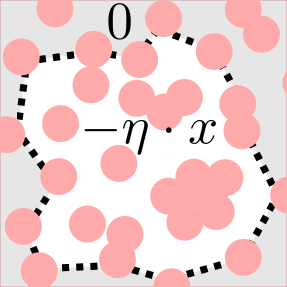
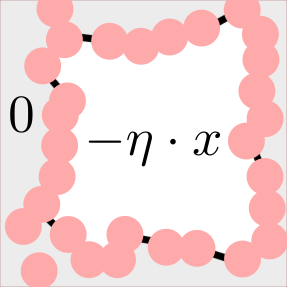
Figure 3: High vs low conductivity. The balls represent $\Xi$. The white area corresponds to $v\approx-\eta\cdot x+const$. Black lines indicate large contributions to $\int_{[0,n]^{d}\backslash\Xi}\big{|}\eta+\nabla v\big{|}^{2}\text{\,$\mathrm{d}$}x$.

We have defined statistical connectedness (11) via the filled-up Boolean model $\boldsymbol{\boxminus}$. Unfortunately, filling up holes is non-local (depending on the size of holes) which is troublesome on the stochastic side. However, an analogue of [KOZ94, Lemma 9.7] tells us that the effective conductivity of both the Boolean model $\Xi$ and its filled-up version $\boldsymbol{\boxminus}$ are the same.

Theorem 52 (Filling up holes preserves the effective conductivity).

For every ergodic admissible point process we have almost surely

$$\eta^{t}\mathcal{A}\eta =\lim_{n\to\infty}n^{-d}\inf_{v\in C_{0}^{\infty}([0,n]^{d})}\int_{[0,n]^{d}\backslash\boldsymbol{\boxminus}}\big{|}\eta-\nabla v\big{|}^{2}=\lim_{n\to\infty}n^{-d}\inf_{v\in C_{0}^{\infty}([0,n]^{d})}\int_{[0,n]^{d}\backslash\Xi}\big{|}\eta-\nabla v\big{|}^{2}\,.$$

Proof.

As mentioned before, this is a variation of [KOZ94, Lemma 9.7] fitted to our purpose. Let

• $K_{n}^{s}$ be the set of islands (i.e. connected components in $\mathbb{R}^{d}\backslash\Xi$ of finite diameter) that intersect but do not lie inside $[0,n]^{d}$ and that are encircled by a $\Xi$-cluster of size at most $s$.

• $L_{n}^{s}$ be the set of islands that do not completely lie inside $[0,n]^{d}$ and that are encircled by a $\Xi$-cluster of size larger than $s$.

All the islands in $K_{n}^{s}$ and $L_{n}^{s}$ belong to connected components of $\mathbb{R}^{d}\backslash\Xi$ different from $\boldsymbol{\boxminus}^{\complement}$ (the unique unbounded connected component). Since $\mathbb{X}$ is admissible, almost surely they all have non-zero distance to $\boldsymbol{\boxminus}^{\complement}$. Therefore, the following infimum decomposes, with all the infima being over $v\in C_{0}^{\infty}([0,n]^{d})$

$$\inf_{v}\int_{[0,n]^{d}\backslash\Xi}\big{|}\eta-\nabla v\big{|}^{2} =\inf_{v}\int_{([0,n]^{d}\backslash\Xi)\backslash(K_{n}^{s}\cup L_{n}^{s})}\big{|}\eta-\nabla v\big{|}^{2}+\inf_{v}\int_{K_{n}^{s}\cup L_{n}^{s}}\big{|}\eta-\nabla v\big{|}^{2}$$

$$=\inf_{v}\int_{([0,n]^{d}\backslash\boldsymbol{\boxminus})\backslash(K_{n}^{s}\cup L_{n}^{s})}\big{|}\eta-\nabla v\big{|}^{2}+\inf_{v}\int_{K_{n}^{s}\cup L_{n}^{s}}\big{|}\eta-\nabla v\big{|}^{2}$$

$$=\inf_{v}\int_{[0,n]^{d}\backslash\boldsymbol{\boxminus}}\big{|}\eta-\nabla v\big{|}^{2}+C\,,$$

with

$$\big{|}C\big{|}\leq\big{|}\eta\big{|}\left[\mathcal{L}^{d}(K_{n}^{s})+\mathcal{L}^{d}(L_{n}^{s})\right]$$

and where the second equality comes from the fact that filling up islands that lie completely inside $[0,n]^{d}$ does not change the value of the infimum. Now, the claim follows from

• $\mathcal{L}^{d}(K_{n}^{s})\sim O(n^{d-1})$ for fixed $s$, so $\lim_{n\to\infty}n^{-d}\mathcal{L}^{d}(K_{n}^{s})=0$ and

• $\lim_{n\to\infty}n^{-d}\mathcal{L}^{d}(L_{n}^{s})=\text{density}(L^{s})$ where $L^{s}$ denotes islands encircled by clusters of size greater than $s$. But

  $$\bigcap_{s\in\mathbb{N}}L^{s}=\emptyset,$$

  so $\lim_{s\to\infty}\text{density}(L^{s})=0$. Choosing $s$ sufficiently large finishes the proof.

∎

6.2 Percolation channels

Definition 53 (Percolation channels (see Figure 4)).

Fix a $k_{\text{$\mathrm{scale}$}}\in\mathbb{N}$. We consider the lattice $\mathbb{Z}_{n}^{d}\subset\mathbb{Z}^{d}$ and the cube with corner $z=(z_{1},\dots,z_{d})\in\mathbb{Z}^{d}$

$$\mathbb{Z}_{n}^{d}: =\mathbb{Z}^{d}\cap[0,n)^{d}\qquad\text{and}\qquad\mathcal{K}_{z}:=\bigtimes_{i=1}^{d}[z_{i},z_{i}+1]$$

and call two vertices $z,z^{\prime}$ neighbors if their $l^{1}$-distance is equal to $1$.
We call $z$ open iff

$$\Xi\cap k_{\text{$\mathrm{scale}$}}^{-1}\mathcal{K}_{z}=\emptyset.$$

An open left-right crossing $\gamma=(z^{(1)},\dots,z^{(l)})$ of $\mathbb{Z}_{n}^{d}$ is called a percolation channel in $\mathbb{Z}_{n}^{d}$, i.e.

1. all the $z^{(i)}$ are open and

2. $z_{1}^{(1)}=0$ and $z_{1}^{(l)}=n-1$.

We define the quantity (depending on the random $\Xi$ and on $k_{\text{$\mathrm{scale}$}}$)

$$\mathbf{N}(n): =\max\big{\{}j\,|\,\gamma_{1},\dots\gamma_{j}\text{ are disjoint percolation channels in }\mathbb{Z}_{n}^{d}\big{\}}$$

$$=\text{"maximal number of disjoint percolation channels in $\mathbb{Z}_{n}^{d}$"}$$

and the tube $L(\gamma)$ corresponding to the path $\gamma=(z^{(1)},\dots,z^{(l)})$ as

$$L(\gamma):=\bigcup_{i\leq l}k_{\text{$\mathrm{scale}$}}^{-1}\mathcal{K}_{z^{(i)}}.$$

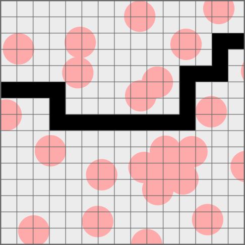
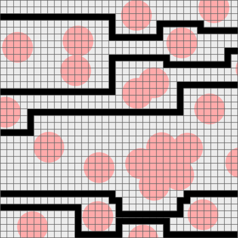
Figure 4: Percolation channels for different $k_{\text{$\mathrm{scale}$}}$

Statistical connectedness of $\mathbb{R}^{d}\backslash\Xi$ then reads as follows:

Theorem 54 (Percolation channels imply conductivity).

For almost every realization $\mathbbm{x}$ of an ergodic admissible point process, we have for $\Xi=\Xi\mathbbm{x}$

$$\lim_{n\to\infty}n^{-d}\inf_{v\in C_{0}^{\infty}([0,n]^{d})}\int_{[0,n]^{d}\backslash\Xi}\big{|}e_{1}-\nabla v\big{|}^{2}\text{\,$\mathrm{d}$}x\geq\limsup_{n\to\infty}\Big{(}\frac{\mathbf{N}(n)}{n^{d-1}}\Big{)}^{2}.$$

In particular, the effective conductivity is strictly positive if almost surely

$$\limsup_{n\to\infty}\frac{\mathbf{N}(n)}{n^{d-1}}>0\,.$$ (27)

Proof.

This is an analogue of [KOZ94, Theorem 9.11] and relies on defining a suitable vector field $\overrightarrow{F}_{\gamma}:\ [0,k_{\text{$\mathrm{scale}$}}^{-1}n]^{d}\to\mathbb{R}^{d}$ inside channels $\gamma=(z^{(1)},\dots,z^{(l)})$ on $\mathbb{Z}_{n}^{d}$. We want $\overrightarrow{F}_{\gamma}$ to satisfy the following

• $\big{|}\overrightarrow{F}_{\gamma}(x)\big{|}=1$ for every $x$ inside the tube $L(\gamma)$ and $\overrightarrow{F}_{\gamma}(x)=0$ outside.

• $\overrightarrow{F}_{\gamma}$ is orthogonal to $\partial L(\gamma)$ except on $\partial L(\gamma)_{-}:=\mathcal{K}_{z^{(1)}}\cap\{x_{1}=0\}$ and $\partial L(\gamma)_{+}:=\mathcal{K}_{z^{(l)}}\cap\{x_{1}=k_{\text{$\mathrm{scale}$}}^{-1}n\}$.

• $\overrightarrow{F}_{\gamma}(x)=e_{1}$ for $x\in\partial L(\gamma)_{-}\cup\partial L(\gamma)_{+}$.

• For the standard normal vector $\nu$ to $\partial L(\gamma)$:

  $$\int_{L(\gamma)}(e_{1}-\nabla v)\cdot\overrightarrow{F}_{\gamma}\text{\,$\mathrm{d}$}x=\int_{\partial L(\gamma)}(x_{1}-v)\overrightarrow{F}_{\gamma}\cdot\nu\text{\,$\mathrm{d}$}x.$$

Figure 5 illustrates how $\overrightarrow{F}_{\gamma}$ can be chosen to satisfy these properties.

The rest is simple. Take $\gamma_{1},\dots\gamma_{\mathbf{N}(n)}$ disjoint non-self-intersecting channels in $\mathbb{Z}_{n}^{d}$. Set

$$T:=\bigcup_{i\leq\mathbf{N}(n)}L(\gamma_{i})\subset[0,k_{\text{$\mathrm{scale}$}}^{-1}n]^{d},\qquad\overrightarrow{F}:=\sum_{i\leq\mathbf{N}(n)}\overrightarrow{F}_{\gamma_{i}}.$$

Then,

$$\int_{[0,k_{\text{$\mathrm{scale}$}}^{-1}n]^{d}\backslash\Xi}\big{|}e_{1}-\nabla v\big{|}^{2}\text{\,$\mathrm{d}$}x \geq\int_{T}\big{|}e_{1}-\nabla v\big{|}^{2}\text{\,$\mathrm{d}$}x\geq\int_{T}\big{|}(e_{1}-\nabla v)\cdot\overrightarrow{F}\big{|}^{2}\text{\,$\mathrm{d}$}x$$

$$\geq\frac{1}{\mathcal{L}^{d}(T)}\left(\int_{T}(e_{1}-\nabla v)\cdot\overrightarrow{F}\text{\,$\mathrm{d}$}x\right)^{2}\geq\frac{k_{\text{$\mathrm{scale}$}}^{d}}{n^{d}}\left(\int_{T}(e_{1}-\nabla v)\cdot\overrightarrow{F}\text{\,$\mathrm{d}$}x\right)^{2}\,.$$

For a fixed tube $L=L(\gamma_{i})$, we have

$$\int_{L}(e_{1}-\nabla v)\cdot\overrightarrow{F}\text{\,$\mathrm{d}$}x =\int_{\partial L}(x_{1}-v)\overrightarrow{F}\cdot\nu\text{\,$\mathrm{d}$}\mathcal{H}^{d-1}(x)=\int_{\partial L_{-}\cup\partial L_{+}}(x_{1}-v)\overrightarrow{F}\cdot\nu\text{\,$\mathrm{d}$}\mathcal{H}^{d-1}(x)$$

$$=\int_{\partial L_{+}}k_{\text{$\mathrm{scale}$}}^{-1}ne_{1}\cdot e_{1}\text{\,$\mathrm{d}$}\mathcal{H}^{d-1}(x)=k_{\text{$\mathrm{scale}$}}^{-1}n\mathcal{H}^{d-1}(\partial L_{+})=k_{\text{$\mathrm{scale}$}}^{-d}n.$$

Figure 5: Using the Gauß divergence theorem on the parts where the vector field is constant only yields contributions from the “starting” surface and the “ending” surface. Whenever the tube makes a left or right turn, we see that the contributions on the diagonal surface cancel out (we have a positive contribution from the incoming part of the tube and a negative contribution from the outgoing one).

Therefore,

$$\int_{[0,k_{\text{$\mathrm{scale}$}}^{-1}n]^{d}\backslash\Xi)}\big{|}e_{1}-\nabla v\big{|}^{2}\text{\,$\mathrm{d}$}x \geq\frac{k_{\text{$\mathrm{scale}$}}^{d}}{n^{d}}\big{(}k_{\text{$\mathrm{scale}$}}^{-d}n\mathbf{N}(n)\big{)}^{2}$$

and so

$$\big{(}k_{\text{$\mathrm{scale}$}}^{-1}n\big{)}^{-d}\int_{[0,k_{\text{$\mathrm{scale}$}}^{-1}n]^{d}\backslash\Xi}\big{|}e_{1}-\nabla v\big{|}^{2}\text{\,$\mathrm{d}$}x\geq\left(\frac{\mathbf{N}(n)}{n^{d-1}}\right)^{2}.$$

Passing to the $\limsup$ finishes the proof. ∎

Remark 55 ($d=2$ and bottom-top crossings).

Let $\mathbf{L}(n)$ be the minimal number of open vertices that a $l^{\infty}$-bottom-top crossing of $\mathbb{Z}_{n}^{2}$ must have. It turns out that in $d=2$

$$\mathbf{L}(n)=\mathbf{N}(n)\,$$

(see 67). We will use this to show LABEL:Eq:Number-of-Channels for the Poisson point process $\mathbb{X}_{\mathrm{poi}}$.

7 Example: Poisson point processes

The driving force behind this work has been a stationary Poisson point process $\mathbb{X}_{\mathrm{poi}}$. It is known that the Poisson point process is ergodic (even mixing) and its high spatial independence makes it the canonical random point process. As pointed out before though, $\Xi\mathbb{X}_{\mathrm{poi}}$ gives rise to numerous analytical issues which prevent the usage of the usual homogenization tools.
The main theorem (50) tells us that homogenization is still reasonable for highly irregular filled-up Boolean models $\boldsymbol{\boxminus}\mathbb{X}$ driven by admissible point processes $\mathbb{X}$.

It is known for $\mathbb{X}_{\mathrm{poi}}$ that there exists some critical radius $r_{c}:=r_{c}[\lambda(\mathbb{X}_{\mathrm{poi}})]\in(0,\,\infty)$ such that

• $\boldsymbol{\boxminus}\mathbb{X}_{\mathrm{poi}}$ only consists of finite clusters for $r<r_{c}$ (subcritical regime) and

• $\boldsymbol{\boxminus}\mathbb{X}_{\mathrm{poi}}$ has a unique infinite cluster for $r>r_{c}$ (supercritical regime).

The behavior at criticality $r=r_{c}$ is still a point of research. For details, we refer to [LP17] for the Poisson point process $\mathbb{X}_{\mathrm{poi}}$ and [MR96, Chapter 3] for the Boolean model $\Xi\mathbb{X}_{\mathrm{poi}}$.

We will see in the subcritical regime that

1. $\mathbb{X}_{\mathrm{poi}}$ is an ergodic admissible point process and

2. $\Xi\mathbb{X}_{\mathrm{poi}}{}^{\complement}$ is statistically connected which is equivalent to $\boldsymbol{\boxminus}\mathbb{X}_{\mathrm{poi}}{}^{\complement}$ being statistically connected (see 52).

We therefore make the following assumption for the rest of this section:

Assumption 56 (subcritical regime).

We assume that

$$r<r_{c}\,.$$

Remark 57 (Scaling relation).

$r_{c}$ has the following scaling relation

$$r_{c}[k^{d}\cdot\lambda(\mathbb{X}_{\mathrm{poi}})]=r_{c}[\lambda(k^{-1}\mathbb{X}_{\mathrm{poi}})]=k^{-1}r_{c}[\lambda(\mathbb{X}_{\mathrm{poi}})]\,.$$

7.1 Admissibility of Poisson point processes

The Mecke–Slivnyak theorem tells us that the Palm probability measure (39) of a stationary Poisson point process is just a Poisson point process with a point added in the origin. This gives us the following lemma:

Lemma 58 (Equidistance property).

The stationary Poisson point process $\mathbb{X}_{\mathrm{poi}}$ satisfies the equidistance property for arbitrary $r>0$, i.e.

$$\mathbb{P}{\left(\exists x,y\in\mathbb{X}_{\mathrm{poi}}\,|\,d(x,y)=2r\right)}=0\,.$$

Proof.

This follows from using the Palm theorem (39) on

$$f(x,\mathbbm{x}):=\sum_{x_{i}\in\mathbbm{x}}\mathds{1}\left\{d(x,x_{i})=2r\right\}$$

and the Mecke–Slivnyak theorem ([LP17, Theorem 9.4]). ∎

Corollary 59 ($\mathbb{X}_{\mathrm{poi}}$ is admissible).

Under 56, $\mathbb{X}_{\mathrm{poi}}$ is an admissible point process.

Proof.

$\mathbb{X}_{\mathrm{poi}}$ is not just ergodic, but even mixing ([LP17, Theorem 8.13]). The equidistance property has been proven in 58. Finiteness of clusters follows from the subcritical regime (56). ∎

7.2 Statistical connectedness for Poisson point processes

Proving the statistical connectedness of $\Xi\mathbb{X}_{\mathrm{poi}}{}^{\complement}$ (11) is much harder and does not immediately follow from readily available results. Our procedure is as follows:

1. We employ the criterion from Section 6. Therefore, we will check that there are sufficiently many percolation channels for $\Xi\mathbb{X}_{\mathrm{poi}}$.

2. Using the spatial independence of the Poisson point process $\mathbb{X}_{\mathrm{poi}}$, we show that it is sufficient to only consider $2$-dimensional slices.

3. We show the statement in $d=2$ using ideas in [Kes82, Chapter 11]. There, the result has been proven for certain iid fields on planar graphs, including $\mathbb{Z}^{2}$.

Additionally to 56, we need sufficient discretization for the percolation channels:

Assumption 60 (Sufficient scaling).

Let $k_{\text{$\mathrm{scale}$}}\in\mathbb{N}$ large enough such that for the critical radius $r_{c}$

$$\frac{1}{2}(r_{c}-r)>\sqrt{d}k_{\text{$\mathrm{scale}$}}^{-1}\,,$$

e.g. $k_{\text{$\mathrm{scale}$}}:=\lceil 2\frac{\sqrt{d}}{r_{c}-r}\rceil+1$.

Definition 61 (Recap and random field $(X_{z})_{z\in\mathbb{Z}^{d}}$).

Recall 53, most importantly

$$\mathbb{Z}_{n}^{i}: =\mathbb{Z}^{i}\cap[0,n)^{i}\qquad\text{and}\qquad\mathcal{K}_{z}:=\bigtimes_{i=1}^{d}[z_{i},z_{i}+1]$$

as well as the notion of percolation channels for $k_{\text{$\mathrm{scale}$}}$ and

$$\mathbf{N}(n): =\text{"maximal number of disjoint percolation channels in $\mathbb{Z}_{n}^{d}$"\,.}$$

We define the random field

$$(X_{z})_{z\in\mathbb{Z}^{d}}:=\Big{(}\mathds{1}\{\Xi\mathbb{X}_{\mathrm{poi}}\cap k_{\text{$\mathrm{scale}$}}^{-1}\mathcal{K}_{z}=\emptyset\}\Big{)}{}_{z\in\mathbb{Z}^{d}}.$$

We say that $z\in\mathbb{Z}^{d}$ is blocked iff $X_{z}=0$ and open iff $X_{z}=1$. (This is consistent with 53.)

Theorem 62 (Percolation channels of the Poisson point process).

Under 56 and 60, there is a $C>0$ such that LABEL:Eq:Number-of-Channels holds, i.e.

$$\mathbb{P}\big{(}\limsup_{n\to\infty}\frac{\mathbf{N}(n)}{n^{d-1}}\geq C\big{)}=1\,.$$

In particular, $\boldsymbol{\boxminus}\mathbb{X}_{\mathrm{poi}}{}^{\complement}$ is statistically connected (see 54).

The rest of the section deals with the proof of 62. It will follow as a direct consequence of 64 (reduction to $d=2$) and 68 (main result for $d=2$) which are given later.

7.2.1 Spatial independence and moving to $d=2$

For disjoint $U_{1},\,U_{2},\dots\,\subset\mathbb{R}^{d}$ and events $A_{i}$ only depending on $\mathbb{X}_{\mathrm{poi}}$ inside $U_{i}$, we know that $(A_{i})_{i}$ is an independent family. This is one of the striking properties of a Poisson point process and we will heavily make use of it. The Boolean model $\Xi\mathbb{X}_{\mathrm{poi}}$ for radius $r$ still retains this property in a slightly weaker form and correspondingly the random field $(X_{z})_{z\in\mathbb{Z}^{d}}$:

Lemma 63 (Independence in large distances).

Let $A,B\subset\mathbb{Z}^{d}$ such that

$$d^{\infty}(A,B):=\min_{z_{a}\in A,z_{b}\in B}\big{\|}z_{b}-z_{a}\big{\|}_{\infty}\geq 2rk_{\text{$\mathrm{scale}$}}+1\,.$$ (28)

Then, $(X_{z})_{z\in A}$ and $(X_{z})_{z\in B}$ are independent.

Proof.

$(X_{z})_{z\in A}$ is only affected by points of $\mathbb{X}_{\mathrm{poi}}$ inside

$$U_{A}:=\bigcup_{z\in A}\mathbb{B}_{r}{\left(k_{\text{$\mathrm{scale}$}}^{-1}\mathcal{K}_{z}\right)}\,.$$

The same holds for $(X_{z})_{z\in B}$ and we check that LABEL:Eq:Distance-For-Independence implies $U_{A}\cap U_{B}=\emptyset$. ∎

Theorem 64 ($2$-dimensional percolation channels imply channel property for $d>2$).

For $\tilde{z}\in\mathbb{Z}^{d-2}$, we define (compare to 53)

$$\mathbf{N}_{\tilde{z}}^{(2)}(n): =\text{"maximal number of disjoint percolation channels in $\mathbb{Z}_{n}^{2}\times\tilde{z}$"\,.}$$

If there are $\tilde{C},\,p_{0}>0$ such that for some $\tilde{z}\in\mathbb{Z}^{d-2}$

$$\limsup_{n\to\infty}\mathbb{P}{\left(\mathbf{N}_{\tilde{z}}^{(2)}(n)\geq\tilde{C}n\right)}>p_{0}>0\,,$$ (29)

then there exists a $C>0$ such that

$$\limsup_{n\to\infty}\mathbb{P}{\left(\mathbf{N}(n)\geq Cn^{d-1}\right)}=\mathbb{P}\big{(}\limsup_{n\to\infty}\frac{\mathbf{N}(n)}{n^{d-1}}\geq C>0\big{)}=1\,.$$

(This proof heavily relies on the independence structure of the Poisson point process, i.e. 63.)

Proof.

$\mathbb{X}_{\mathrm{poi}}$ is stationary, so for distinct $\tilde{z}_{1},\,\tilde{z}_{2}\in\mathbb{Z}^{d-2}$

$$p(n):=\mathbb{P}{\left(\mathbf{N}_{\tilde{z}_{1}}^{(2)}(n)\geq\tilde{C}n\right)}=\mathbb{P}{\left(\mathbf{N}_{\tilde{z}_{2}}^{(2)}(n)\geq\tilde{C}n\right)}.$$

Let $k:=\lceil 2rk_{\text{$\mathrm{scale}$}}\rceil+1$. By 63, the events on $\mathbb{Z}^{2}\times(k\tilde{z}_{1})$ are independent from the events on $\mathbb{Z}^{2}\times(k\tilde{z}_{2})$. Therefore, $\big{(}\mathds{1}\{\mathbf{N}_{k\tilde{z}}^{(2)}(kn)\geq\tilde{C}n\}\big{)}_{\tilde{z}\in\mathbb{Z}^{d-2}}$ is an iid family of Bernoulli random variables with parameter $p(n)$. Then,

$$\mathbb{P}\big{(}\mathbf{N}(kn) \geq\frac{\tilde{C}p_{0}}{2k^{d-2}}(kn)^{d-1}\big{)}$$

$$\geq \mathbb{P}\big{(}\text{For at least $\frac{1}{2}p_{0}$ of the }\tilde{z}\in\mathbb{Z}_{n}^{(d-2)}:\ \mathbf{N}_{\tilde{z}}^{(2)}(kn)\geq\tilde{C}kn\big{)}$$

$$= \mathbb{P}\Big{(}\frac{1}{\#\mathbb{Z}_{n}^{(d-2)}}\sum_{\tilde{z}\in\mathbb{Z}_{n}^{(d-2)}}\mathds{1}\{\mathbf{N}_{k\tilde{z}}^{(2)}(kn)\geq\tilde{C}n\}\geq\frac{1}{2}p_{0}\Big{)}\,.$$

By LABEL:Eq:Number-Percolation-Channels-D=00003D2 and the law of large numbers, we get

$$\limsup_{n\to\infty}\mathbb{P}\big{(}\mathbf{N}(n)\geq\frac{\tilde{C}p_{0}}{2k^{d-2}}n{}^{d-1}\big{)}\geq\limsup_{n\to\infty}\mathbb{P}\big{(}\mathbf{N}(kn)\geq\frac{\tilde{C}p_{0}}{2k^{d-2}}(kn)^{d-1}\big{)}=1\,.$$

Setting $C=\frac{\tilde{C}p_{0}}{2k^{d-2}}$, we obtain LABEL:Eq:Number-of-Channels after checking

$$\mathbb{P}\big{(}\limsup_{n\to\infty}\frac{\mathbf{N}(n)}{n^{d-1}}\geq C\big{)}=\limsup_{n\to\infty}\mathbb{P}\big{(}\frac{\mathbf{N}(n)}{n^{d-1}}\geq C\big{)}=1$$

which finishes the proof. ∎

Remark 65.

Spatial independence is needed to move from $d=2$ to $d\geq 3$. The strong independence properties of $\mathbb{X}_{\mathrm{poi}}$ allow far weaker conditions on $\mathbf{N}^{(2)}(n)$ (positive probability) than on $\mathbf{N}(n)$ (probability 1). Either way, 68 shows that $\mathbb{P}(\mathbf{N}^{(2)}(n)<Cn)$ drops exponentially in $n$.

7.2.2 $d=2$: Definitions and preliminary results

As shown before, we may limit ourselves to a fixed lattice $\mathbb{Z}^{2}\times 0_{\mathbb{Z}^{d-2}}\simeq\mathbb{Z}^{2}$. Therefore, we will often suppress the “anchor point” $0_{\mathbb{Z}^{d-2}}$ and just act like we are in $\mathbb{Z}^{2}$. Our random field from 61 is then by abuse of notation

$$(X_{z})_{z\in\mathbb{Z}^{2}}\simeq(X_{z})_{z\in\mathbb{Z}^{2}\times 0_{\mathbb{Z}^{d-2}}}\,.$$

Definition 66 (Vertical crossings).

Consider the $(\mathbb{Z}^{2},l^{\infty})$-lattice, that is $z,z^{\prime}$ are neighbors iff $\big{\|}z-z^{\prime}\big{\|}_{\infty}=1$.
An $l^{\infty}$-bottom-top crossing in $\mathbb{Z}_{n}^{2}$ is called a vertical crossing. We call a path blocked iff all its vertices are blocked. We define the quantity

$$\mathbf{L}(n):=\text{"minimal number of open vertices in a vertical crossing in $\mathbb{Z}_{n}^{2}$"}.$$

(The percolation channels lie on the $l^{1}$-graph, while the vertical crossings lie on the $l^{\infty}$-graph.)

We may work with single vertical crossings instead of collections of percolation channels:

Lemma 67 (Percolation channels vs vertical crossings (see Figure 6)).

It holds that

$$\mathbf{N}(n)=\mathbf{L}(n).$$

Proof.

See the proof of [Kes82, Theorem 11.1] based on Menger’s Theorem and [Kes82, Proposition 2.2]. ∎

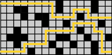
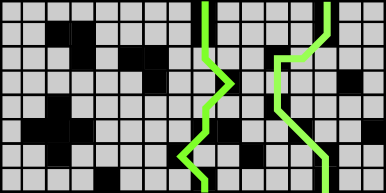
Figure 6: Disjoint percolation channels vs.~vertical crossings. On the left side, we see that we can only have at most two $l^{1}$-channels. The right figure shows that any $l^{\infty}$-vertical crossing must contain at least two open vertices.

The main work is proving the following equivalent of [Kes82, Proposition 11.1]:

Theorem 68 (Open vertices in vertical crossings).

Under 56 and 60, there are $C_{i}>0$ such that

$$\mathbb{P}\big{(}\exists o\leadsto\mathbb{Z}\times\{n\}\text{ with at most }C_{1}n\text{ open vertices}\big{)}\leq C_{2}\exp\big{(}-C_{3}n\big{)}\,,$$

in particular

$$\mathbb{P}\big{(}\mathbf{N}(n)\geq C_{1}n\big{)}\geq 1-C_{2}n\exp(-C_{3}n)\,.$$

The proof relies on a reduction scheme of the path $\gamma:\ o\leadsto\mathbb{Z}\times\{n\}$. We divide $\gamma$ into several segments which must either contain an open vertex or contain a blocked path of large diameter. Since we are in the subcritical regime, the probability of such paths decreases exponentially in their diameter:

Lemma 69 (Diameter of blocked paths).

Let $z\in\mathbb{Z}^{2}$. Under 56 and $k_{\text{$\mathrm{scale}$}}\in\mathbb{N}$ as in 60, there are $C_{i}>0$ such that

$$\mathbb{P}\big{(}\exists\text{blocked path }\gamma,\,z\in\gamma,\,\mathrm{diam}(\gamma)\geq n\big{)}\leq C_{1}\exp\big{(}-C_{2}n\big{)}\,,$$

where

$$\mathrm{diam}(\gamma):=\max_{z_{1},z_{2}\in\gamma}\big{\|}z_{1}-z_{2}\big{\|}_{2}\,.$$

Proof.

Consider the Boolean model for radius $R:=\frac{1}{2}(r+r_{c})<r_{c}$, i.e.

$$\Xi^{(R)}\mathbb{X}_{\mathrm{poi}}:=\mathbb{B}_{R}{\left(\mathbb{X}_{\mathrm{poi}}\right)}\,.$$

Let $\gamma=(z^{(1)},\dots,z^{(l)})$ be a blocked path in $\mathbb{Z}^{2}$ containing $z$ with diameter $\geq n$. Since $\gamma$ is blocked and $R-r>\sqrt{d}k_{\text{$\mathrm{scale}$}}^{-1}$ (60), we find for every $1\leq i\leq l$ some $x_{i}\in\mathbb{X}_{\mathrm{poi}}$ such that

$$\mathcal{K}_{z^{(i)}}\cap k_{\text{$\mathrm{scale}$}}\mathbb{B}_{r}{\left(x_{i}\right)}\neq\emptyset$$

and therefore

$$\mathcal{K}_{z^{(i)}}\subset k_{\text{$\mathrm{scale}$}}\mathbb{B}_{R}{\left(x_{i}\right)}\,.$$

Connecting all the $z^{(i)}$ by a straight line, we obtain a continuous path inside $k_{\text{$\mathrm{scale}$}}\Xi^{(R)}\mathbb{X}_{\mathrm{poi}}$. In particular, they all belong to the same $k_{\text{$\mathrm{scale}$}}\Xi^{(R)}\mathbb{X}_{\mathrm{poi}}$-cluster. Then,

$$\mathbb{P}\big{(}\exists \text{closed path }\gamma,\,z\in\gamma\text{ and }\mathrm{diam}(\gamma)\geq n\big{)}$$

$$\leq\mathbb{P}\big{(}z\text{ lies in a cluster in }k_{\text{$\mathrm{scale}$}}\Xi^{(R)}\mathbb{X}_{\mathrm{poi}}\text{ of diameter }\geq n\big{)}$$

$$\leq C_{1}\exp(-C_{2}n)$$

since the occurrence of large clusters drops exponentially in their diameter ([MR96, Lemma 2.4]). ∎

7.2.3 Proof of 68 (open vertices in vertical crossings)

Let $n\in\mathbb{N}$. As pointed out before, follow the procedure in [Kes82, Proposition 11.1] but fitted to the continuum setting. We define $A(z,k)$ for $z\in\mathbb{Z}^{2}$ and $k\in\mathbb{N}$ as

$$A(z,k):=\big{\{} \exists l^{\infty}\text{-path }z\leadsto\mathbb{Z}\times\{n\}\text{ with at most }k\text{ open vertices}\big{\}}.\text{ }$$

The idea is to break up the path $o\leadsto\mathbb{Z}\times\{n\}$ into multiple segments (see LABEL:Fig:Path-Decomposition). In each segment, we can either reduce $k$ by $1$ or employ 69. We set

$$\tilde{s}: =\lceil 2rk_{\text{$\mathrm{scale}$}}\rceil+1$$

$$B_{1}^{\infty}(z,s): =\big{\{}v\in\mathbb{Z}^{2}\,|\,\big{\|}z-v\big{\|}_{\infty}\leq s\big{\}}$$

$$B_{2}^{\infty}(z,s): =\big{\{}v\in\mathbb{Z}^{2}\,|\,\big{\|}z-v\big{\|}_{\infty}\leq s+\tilde{s}\big{\}}$$

$$D^{\infty}(z,s): =\big{\{}v\in\mathbb{Z}^{2}\,|\,\big{\|}z-v\big{\|}_{\infty}=s+\tilde{s}+1\big{\}}="\text{boundary of }B_{2}^{\infty}(z,s)"\,.$$

These boxes are defined so that the following holds: For fixed $z\in\mathbb{Z}^{2}$, we have by 63 that the random variables $(X_{v})_{v\in B_{1}^{\infty}(z,s)}$ and $(X_{v})_{v\in\mathbb{Z}^{2}\backslash B_{2}^{\infty}(z,s)}$ are independent. That means the state of the vertices in $B_{1}^{\infty}(z,s)$ is independent from the state of the vertices in $\mathbb{Z}^{2}\backslash B_{2}^{\infty}(z,s)=B_{2}^{\infty}(z,s)^{\complement}$. Additionally, we define the probability

$$g(z,s):= \mathbb{P}\big{(}\exists z\leadsto B_{1}^{\infty}(z,s)^{\complement}\text{ blocked inside }B_{1}^{\infty}(z,s)\big{)}.$$

The key inequality for the iteration in $k$ is the following

$$\mathbb{P}\big{(}A(z,k)\big{)}\leq\sum_{v\in D^{\infty}(z,s)}\Big{[}g(z,s)\mathbb{P}\big{(}A(v,k)\big{)}+\mathbb{P}\big{(}A(v,k-1)\big{)}\Big{]}$$ (30)

for $z=(z_{1},z_{2})\in\mathbb{Z}^{2}$ whenever $z_{2}<n-(s+\tilde{s})$.

Proof of LABEL:Eq:Kesten-Iteration.

Consider the event that for some $v\in D^{\infty}(z,s)$, we find a path $v\leadsto\mathbb{Z}\times\{n\}$ that has at most $k-1$ open vertices, i.e.

$$E:=\bigcup_{v\in D^{\infty}(z,s)}A(v,k-1)\,.$$

Now assume that the event $A(z,k)\backslash E$ happens. Take a path $\gamma=(z,v^{(1)},\dots,v^{(j)})$ with $v_{2}^{(j)}=n$ and at most $k$ of the $v^{(i)}$ being open. Let $i_{1}$ be the last index with $v^{(i_{1})}\in D^{\infty}(z,s)$. This $i_{1}$ exists since $z_{2}<n-(s+\tilde{s})$, so $\gamma$ has to pass by $D^{\infty}(z,s)$ to reach $\mathbb{Z}\times\{n\}$. For this $i_{1}$, we know that $(v^{(i_{1})},\dots v^{(j)})$ completely lies in $B_{2}^{\infty}(z,s)^{\complement}$. Since $E$ does not happen, it must have $k$ open vertices. $(z,v^{(1)},\dots,v^{(i_{1})})$ is a path from $z$ to $B_{1}^{\infty}(z,s)^{\complement}$ that is blocked everywhere except its end. Therefore,

$$A(z,k)\backslash E\subset\bigcup_{v\in D^{\infty}(z,s)}\big{\{} \exists z\leadsto B_{1}^{\infty}(z,s)^{\complement}\text{ blocked in }B_{1}^{\infty}(z,s)\text{ and}$$

$$\exists v\leadsto\mathbb{Z}\times\{n\}\text{ in }B_{2}^{\infty}(z,s)^{\complement}\text{ with }\text{at most }k\text{ open vertices}\big{\}}.$$

As mentioned before, the events in $B_{1}^{\infty}(z,s)$ and $B_{2}^{\infty}(z,s)^{\complement}$ are independent from each other. This gives us

$$\mathbb{P}\big{(}A(z,k)\backslash E\big{)}\leq\sum_{v\in D^{\infty}(z,s)}\mathbb{P}\big{(} \exists z\leadsto B_{1}^{\infty}(z,s)^{\complement}\text{ blocked in }B_{1}^{\infty}(z,s)\text{ and}$$

$$\exists v\leadsto\mathbb{Z}\times\{n\}\text{ in }B_{2}^{\infty}(z,s)^{\complement}\text{ with }\text{at most }k\text{ open vertices}\big{)}$$

$$=\sum_{v\in D^{\infty}(z,s)}\mathbb{P}\big{(} \exists z\leadsto B_{1}^{\infty}(z,s)^{\complement}\text{ blocked in }B_{1}^{\infty}(z,s)\big{)}$$

$$\times\mathbb{P}\big{(} \exists v\leadsto\mathbb{Z}\times\{n\}\text{ in }B_{2}^{\infty}(z,s)^{\complement}\text{ with }\text{at most }k\text{ open vertices}\big{)}$$

$$\leq\sum_{v\in D^{\infty}(z,s)}g( z,s)\mathbb{P}\big{(}A(v,k)\big{)}.$$

$$\mathbb{P}\big{(}A(z,k)\big{)} \leq\mathbb{P}\big{(}A(z,k)\backslash E\big{)}+\mathbb{P}(E)\leq\sum_{v\in D^{\infty}(z,s)}\Big{[}g(z,s)\mathbb{P}\big{(}A(v,k)\big{)}+\mathbb{P}\big{(}A(v,k-1)\big{)}\Big{]}$$

concludes the proof of LABEL:Eq:Kesten-Iteration. ∎

Figure 7: $B_{1}^{\infty},\,B_{2}^{\infty},\,D^{\infty}$ and decomposition of paths (left-right crossing instead of top-bottom)

Observe that the reduction in $k$ can only happen until $k=0$, so more $g(z,s)$-terms have to show up at some point. Since any path $z\leadsto B_{1}^{\infty}(z,s)^{\complement}$ has diameter of at least $s$, 69 tells us that $g(z,s)\leq C_{1}\exp\big{(}-C_{2}s\big{)}$ for $C_{1},\,C_{2}>0$ independent of $z$ and $s$. Choose $s$ large such that

$$g(z,s)\cdot\#D^{\infty}(z,s) \leq C_{1}\exp\big{(}-C_{2}s\big{)}\,\cdot 8(s+\tilde{s}+1)\leq\frac{1}{4}.$$

For simplicity, we introduce

$$D^{\infty} :=D^{\infty}(o,s)\qquad\text{and}\qquad h(z,y):=\begin{cases}g(z,s)&\text{if }y=0\\ 1&\text{if }y=1.\end{cases}$$

and rewrite LABEL:Eq:Kesten-Iteration into

$$\mathbb{P}\big{(}A(z,k)\big{)} \leq\sum_{v^{(1)}\in D^{\infty},\,y_{1}\in\{0,1\}}h(z,y_{1})\mathbb{P}\big{(}A(z+v^{(1)},k-y_{1})\big{)}\,.$$ (31)

We now iteratively use LABEL:Eq:Kesten-Iteration-2 up to $l$ times as it is only applicable when $z_{2}<n-(s+\tilde{s})$. All the $v^{(i)}$ are summed over $D^{\infty}$ and all the $y_{i}$ over $\{0,1\}$.

$$\mathbb{P}\big{(}A (o,k)\big{)}$$

$$\leq\ \ \sum_{\begin{subarray}{c}i\leq l,v^{(i)},y_{i}\\ v_{2}^{(1)}+\dots+v_{2}^{(l)}<n-(s+\tilde{s})\\ y_{1}+\dots+y_{l}\leq k\end{subarray}}\mathbb{P}(A(v^{(1)}+\dots+v^{(l)},k-y_{1}-\dots-y_{l}))\prod_{m\leq l}h(v^{(1)}+\dots+v^{(m-1)},y_{m})$$

$$+ \sum_{\frac{n-(s+\tilde{s})}{s+\tilde{s}+1}\leq j\leq l}\sum_{\begin{subarray}{c}i\leq j,v^{(i)},y_{i}\\ v_{2}^{(1)}+\dots+v_{2}^{(j-1)}<n-(s+\tilde{s})\\ v_{2}^{(1)}+\dots+v_{2}^{(j)}\geq n-(s+\tilde{s})\\ y_{1}+\dots+y_{j}\leq k\end{subarray}}\mathbb{P}(A(v^{(1)}+\dots+v^{(j)},k-y_{1}-\dots-y_{j}))\prod_{m\leq j}h(v^{(1)}+\dots+v^{(m-1)},y_{m})$$

$$\leq\ \ \sum_{\begin{subarray}{c}y_{1},\dots,y_{l}\\ y_{1}+\dots+y_{l}\leq k\end{subarray}}\Big{(}\#D^{\infty}\sup_{\begin{subarray}{c}v\in\mathbb{Z}^{2}\\ v_{2}<n-(s+\tilde{s})\end{subarray}}h(v,y_{m})\Big{)}^{l}+\sum_{\frac{n-(s+\tilde{s})}{s+\tilde{s}+1}\leq j\leq l}\sum_{\begin{subarray}{c}y_{1},\dots,y_{j}\\ y_{1}+\dots+y_{j}\leq k\end{subarray}}\Big{(}\#D^{\infty}\sup_{\begin{subarray}{c}v\in\mathbb{Z}^{2}\\ v_{2}<n-(s+\tilde{s})\end{subarray}}h(v,y_{m})\Big{)}^{j}$$

We iterate as long as $0+v_{2}^{(1)}+\dots v_{2}^{(j)}<n-(s+\tilde{s})$, otherwise we stop for $0+v_{2}^{(1)}+\dots v_{2}^{(j)}$ and land in the second summand. Only $y_{1}+\dots+y_{j}\leq k$ matters since $A(z,m)=0$ whenever $m<0$. Also observe that $v_{2}^{(1)}+\dots+v_{2}^{(j)}\geq n-(s+\tilde{s})$ can only happen if

$$j\geq\frac{n-(s+\tilde{s})}{s+\tilde{s}+1}$$

since we “gain” at most $s+\tilde{s}+1$ to the second component in each $v^{(i)}$.
Let $\alpha>0$ be large enough such that

$$\phi(\alpha): =\sum_{y\in\{0,1\}}\sup_{\begin{subarray}{c}z\in\mathbb{Z}^{2}\\ z_{2}<n-(s+\tilde{s})\end{subarray}}\#D^{\infty}\cdot h(z,y)\cdot e^{-\alpha y}\leq\frac{1}{4}+\#D^{\infty}\cdot e^{-\alpha}\leq\frac{1}{2}.$$

Then,

$$\mathbb{P}\big{(}A(o,k)\big{)}\leq\ \ e^{\alpha k}\sum_{\begin{subarray}{c}y_{1},\dots,y_{l}\\ y_{1}+\dots+y_{l}\leq k\end{subarray}}\Big{(}\#D^{\infty}\sup_{\begin{subarray}{c}v\in\mathbb{Z}^{2}\\ v_{2}<n-(s+\tilde{s})\end{subarray}}h(v,y_{m})\Big{)}^{l}\prod_{i\leq l}e^{-\alpha y_{i}}$$

$$+ e^{\alpha k}\sum_{\frac{n-(s+\tilde{s})}{s+\tilde{s}+1}\leq j\leq l}\sum_{\begin{subarray}{c}y_{1},\dots,y_{j}\\ y_{1}+\dots+y_{j}\leq k\end{subarray}}\Big{(}\#D^{\infty}\sup_{\begin{subarray}{c}v\in\mathbb{Z}^{2}\\ v_{2}<n-(s+\tilde{s})\end{subarray}}h(v,y_{m})\Big{)}^{j}\prod_{i\leq j}e^{-\alpha y_{i}}$$

$$\leq\ \ e^{\alpha k}\phi(\alpha)^{l}+e^{\alpha k}\sum_{j\geq\frac{n-(s+\tilde{s})}{s+\tilde{s}+1}}^{l}\phi(\alpha)^{j}\leq e^{\alpha k}\big{[}2^{-l}+2^{-\frac{n-(s+\tilde{s})}{s+\tilde{s}+1}+1}\big{]}\,.$$

Since $l\in\mathbb{N}$ was arbitrary, we get

$$\mathbb{P}\big{(}A(o,k)\big{)} \leq e^{\alpha k}\cdot 2^{-\frac{n-(s+\tilde{s})}{s+\tilde{s}+1}+1}=e^{\alpha k-\big{[}\frac{n-(s+\tilde{s})}{s+\tilde{s}+1}-1\big{]}\ln 2}=C_{3}e^{\alpha k-C_{4}n}.$$

Now we finally make use of $k$. Setting $C_{5}:=\frac{C_{4}}{2\alpha}$ and $k:=C_{5}n$, we obtain the claim

$$\mathbb{P}\big{(}A(o,C_{5}n)\big{)}\leq C_{3}\exp\big{(}-\frac{1}{2}C_{4}n\big{)}\,.$$

Acknowledgement.

This work was funded by the German Leibniz Association via the Leibniz Competition 2020.

References

- [All92] G. Allaire. Homogenization and two-scale convergence. SIAM Journal on Mathematical Analysis, 23(6):1482–1518, 1992.
- [DVJ08] D.J. Daley and D. Vere-Jones. An introduction to the theory of point processes. Vol. II. Probability and its Applications (New York). Springer, New York, second edition, 2008. General theory and structure.
- [Fag08] A. Faggionato. Random walks and exclusion processes among random conductances on random infinite clusters: homogenization and hydrodynamic limit. Electronic Journal of Probability, 13:2217–2247, 2008.
- [FHL20] B. Franchi, M. Heida, and S. Lorenzani. A mathematical model for Alzheimer’s disease: An approach via stochastic homogenization of the Smoluchowski equation. Accepted by Communications in Mathematical Sciences, preprint arXiv:1904.11015, 2020.
- [FHS19] F. Flegel, M. Heida, and M. Slowik. Homogenization theory for the random conductance model with degenerate ergodic weights and unbounded-range jumps. 55(3):1226–1257, 2019.
- [GH20] A. Giunti and R.M. Höfer. Convergence of the pressure in the homogenization of the stokes equations in randomly perforated domains. preprint arXiv:2003.04724, 2020.
- [GK15] N. Guillen and I. Kim. Quasistatic droplets in randomly perforated domains. Archive for Rational Mechanics and Analysis, 215(1):211–281, 2015.
- [Hei21] M. Heida. Stochastic homogenization on perforated domains I–Extension operators. preprint arXiv:2105.10945, 2021.
- [HNV21] M. Heida, S. Neukamm, and M. Varga. Stochastic homogenization of -convex gradient flows. Discrete & Continuous Dynamical Systems-S, 14(1):427–453, 2021.
- [Kes82] H. Kesten. Percolation theory for mathematicians, volume 194. Springer, 1982.
- [Koz79] S.M. Kozlov. Averaging of random operators. Matematicheskii Sbornik, 151(2):188–202, 1979.
- [KOZ94] S.M. Kozlov, O.A. Oleinik, and V.V. Zhikov. Homogenization of differential operators and integral functionals. Springer Berlin, Germany, 1994.
- [LP17] G. Last and M. Penrose. Lectures on the Poisson process, volume 7. Cambridge University Press, 2017.
- [Mat86] B. Matérn. Spatial variation, volume 36 of Lecture Notes in Statistics. Springer Berlin, Germany, second edition, 1986. With a Swedish summary.
- [Mec67] J. Mecke. Stationäre zufällige maße auf lokalkompakten abelschen gruppen. Probability Theory and Related Fields, 9(1):36–58, 1967.
- [MP07] P. Mathieu and A. Piatnitski. Quenched invariance principles for random walks on percolation clusters. Proceedings of The Royal Society of London. Series A. Mathematical, Physical and Engineering Sciences, 463(2085):2287–2307, 2007.
- [MR96] R. Meester and R. Roy. Continuum percolation, volume 119. Cambridge University Press, 1996.
- [Ngu89] G. Nguetseng. A general convergence result for a functional related to the theory of homogenization. SIAM Journal on Mathematical Analysis, 20:608–623, 1989.
- [NV18] S. Neukamm and M. Varga. Stochastic unfolding and homogenization of spring network models. Multiscale Modeling & Simulation, 16(2):857–899, 2018.
- [PP20] A. Piatnitski and M. Ptashnyk. Homogenization of biomechanical models of plant tissues with randomly distributed cells. Nonlinearity, 33(10):5510–5542, 2020.
- [PV81] G.C. Papanicolaou and S.R.S. Varadhan. Boundary value problems with rapidly oscillating random coefficients. In Random fields, Vol. I, II (Esztergom, 1979), volume 27 of Colloq. Math. Soc. János Bolyai, pages 835–873. North-Holland, Amsterdam-New York, 1981.
- [Sim86] J. Simon. Compact sets in the space . Annali di Matematica pura ed applicata, 146(1):65–96, 1986.
- [SKM87] D. Stoyan, W.S. Kendall, and J. Mecke. Stochastic geometry and its applications. Wiley Series in Probability and Mathematical Statistics: Applied Probability and Statistics. John Wiley & Sons, Ltd., Chichester, 1987.
- [Ste16] E.M. Stein. Singular integrals and differentiability properties of functions (PMS-30), Volume 30. Princeton university press, 2016.
- [Zhi93] V.V. Zhikov. Averaging in perforated random domains of general type. Mathematical Notes, 53(1):30–42, 1993.
- [Zhi00] V.V. Zhikov. On an extension of the method of two-scale convergence and its applications. Sbornik: Mathematics, 191(7):973–1014, 2000.
- [ZP06] V.V. Zhikov and A.L. Pyatniskii. Homogenization of random singular structures and random measures. Izv. Math., 70(1):19–67, 2006.