1 Introduction

Double holography has drawn much attention recently, which plays an important role in recovering Page curve of Hawking radiation [4, 5, 6]. See also [7, 8, 9, 10, 11, 12, 13, 14, 15, 16, 17, 18, 19, 20, 21, 22, 23, 24, 25, 26, 27, 28, 29, 30, 31, 32] for related works. Double holography is a generalization of the AdS/CFT correspondence [33, 34, 35] and is closely related to brane world holography [36, 37, 38] and AdS/BCFT [39, 40, 41], [2, 3, 42]. Here BCFT means a conformal field theory defined on a manifold with a boundary, where suitable boundary conditions (BC) are imposed [43, 44]. Recently, a novel doubly holographic model called wedge holography has been proposed [45, 46]. For one novel class of solutions, it has been shown that wedge holography is equivalent to AdS/CFT with Einstein gravity [47]. Generally, wedge holography can be obtained as a special limit of AdS/BCFT with edge modes living on the corner of the wedge [45]. Generalizing wedge holography to codim-$m$ defects, [48] proposes the so-called cone holography.

Due to the importance of AdS/BCFT itself and the prominent role it plays in various other dualities as discussed above, any deeper understanding of AdS/BCFT will be quite interesting. At the level of classical gravity, the action for AdS/BCFT is given by

$$I=\int_{N}d^{d+1}x\sqrt{|g|}(R-2\Lambda)+2\int_{Q}d^{d}y\sqrt{|h|}(K-T)$$ (1)

where $K$ is the extrinsic curvature, $T$ is the tension of end-of-the-world brane $Q$ and $h_{ij}$ is the induced metric on $Q$. Taking the variations and focusing on the boundary terms, we have

$$\delta I=-\int_{Q}d^{d}y\sqrt{|h|}\left(K^{ij}-(K-T)h^{ij}\right)\delta h_{ij}=0$$ (2)

in order to have a well-defined action principle (2). The original proposal of Takayanagi [39] is to take on $Q$ the Neumann boundary condition (NBC)

$$\text{NBC}:\ \left(K^{ij}-(K-T)h^{ij}\right)|_{Q}=0.$$ (3)

The Neumann boundary condition imposes conditions on the end-of-the-world brane $Q$ [39, 40, 41] as well as the bulk Einstein metric [49]. In addition, it is possible to impose alternative boundary conditions for AdS/BCFT. For example, we have the conformal boundary condition (CBC) [2, 3], which fixes the conformal geometry of the boundary and the trace of the extrinsic curvature

$$K=\frac{d}{d-1}T,$$ (4a)

$$\delta h_{ij}|_{Q}=2\sigma(y)h_{ij}|_{Q},$$ (4b)

where $\sigma(y)$ is an arbitrary conformal factor. One can also impose the Dirichlet boundary condition (DBC) [42]

$$\text{DBC}:\ \delta h_{ij}|_{Q}=0.$$ (5)

All of these boundary conditions define consistent theory of AdS/BCFT. See also [50, 51, 52, 53, 54] for some early works on the boundary condition of the gravity.

To see that the CBC works, it is instructive to rewrite (2) as

$$\int_{Q}d^{d}y\sqrt{|h|}\big{[}(T-\frac{d-1}{d}K)\delta h+\bar{K}^{ij}\delta h_{ij}\big{]}=0,$$ (6)

where $\delta h=h^{ij}\delta h_{ij}$ is the trace of metric variations and $\bar{K}^{ij}:=K^{ij}-\frac{K}{d}h^{ij}$ is the traceless part of the extrinsic curvature. Since $\bar{K}^{ij}\delta h_{ij}=2\sigma\bar{K}^{ij}h_{ij}=0$, it is clear that the CBC (4) makes vanish the action variation (6). It should be mentioned that the CBC (4) has been partially discussed in [2, 3], which was called mixed BC there. However, [2, 3] have mainly focused on the constraint (4a) without paying much attention to the second condition (4b). In this paper, we will study carefully the complete CBC in order to gain further insights on AdS/BCFT with CBC.

CBC is not just a possible boundary condition for AdS/BCFT, it is actually a very interesting class of boundary condition for a good reason. At the quantum level, one hopes the boundary condition of gravity to be elliptic so that it leads to a well-defined perturbation theory of ‘quantum gravity’ [1]. According to Witten [1], in general DBC is not elliptic and does not lead to a well-defined perturbation theory. It is better-behaved if the extrinsic curvature of the boundary is positive- or negative-definite. This additional condition indeed plays an important role in AdS/BCFT with DBC, which helps to select the correct solutions with positive brane tensions [42]. On the other hand, CBC is always elliptic and leads to a well-defined perturbation theory [1]. Thus it is interesting to consider AdS/BCFT with CBC and investigate the properties of the gravitational perturbations in this context. This is the main motivation of this paper.

The analysis of AdS/BCFT with CBC is however a little more subtle. As originally suggested in [41] and fully developed in [49], it has been shown that while the traditional construction of the bulk metric based on the Fefferman-Graham (FG) expansion does not work for AdS/BCFT due to the existence of junction, a construction of the bulk metric based on a perturbative expansion in the extrinsic curvature works fine. This method has been applied for the case of NBC [49] and DBC [42] with the bulk metric constructed correspondingly, leading to well-defined AdS/BCFT with NBC and DBC. However, it has been observed that the employment of CBC (4) does not fix all the integral constants in the bulk metric solution of the Einstein equations . This is puzzling and appears to be an obstacle to the construction of a well-defined theory of AdS/BCFT based on CBC. In this paper, we resolve this problem and show that CBC also fixes the bulk metric completely and give rises to a well-defined AdS/BCFT. We observe that the metric ansatz employed in [42, 49] admits a non-vanishing extrinsic curvature $k_{ij}$ for the boundary metric of BCFT. For simplicity, we have considered a constant $k_{ij}$ and that was sufficient for the analysis there since the NBC and DBC were already nontrivial at the considered linear perturbative order. However, as the CBC involves higher power of derivatives in the boundary metric, it becomes trivial at the linear perturbative order and this is why the CBC appears to be less restrictive. In this paper, we construct the metric ansatz with non-constant $k_{ij}$ and show that the CBC does fix the bulk metric completely as the case of NBC and DBC. As a result, all the boundary central charges of the Weyl anomaly are also determined.

Let us summarize the main results of this paper. We investigate AdS/BCFT with CBC in this paper. We resolve a subtly related to the application of the CBC to the bulk metric ansatz that has been shown to work well previously for NBC and DBC. We fix the central charges of boundary Weyl anomaly for AdS/BCFT with CBC. It is found that the central charge, which is related to the norm of displacement operator, is the exactly the same for CBC and DBC. Although the central charges are same, the locations of end-of-the-world branes are different for these two AdS/BCFT. We study the dynamics of the metric perturbations with CBC, DBC or NBC imposed on the end-of-the-world branes. At the linear order, the perturbations obey EOM of massive gravity with a mass square spectrum that is discrete and positive. The perturbation modes are obtained by imposing a gauge fixing condition. They can be quantized covariantly by utilizing the BRST method with the inclusion of ghost fields. As shown in [1], the resulting kinetic operators in the BRST invariant action are elliptic. It is in this sense that these fluctuations lead to a well-defined perturbative theory of gravity at the quadratic order. As application, we also briefly discuss the potential implications of the fluctuations, such as the two-point function and the relation to massive islands [13, 24].

We emphasis that in AdS/BCFT, the boundary condition is defined with a one side end-of-the-world brane, i.e. there is nothing beyond it. This is in contrast with the consideration in the Randall-Sundrum (RS) brane world theory where the RS brane is situated in a bulk spacetime and a junction condition is imposed instead. To get to a BCFT, one needs to perform an orbifolding to get to a one-sided setup. Apart from giving an extra factor of 2 in the equation of motion for $Q$ in the case of NBC and CBC, it also has implication on the localization of gravitons due to the rise of a volcano potential localized on the RS brane. Although it is not directly related to the study of AdS/BCFT, the set up is similar and we have performed a study of the problem of localization of gravitons in the brane world setup. Interestingly we find that, for NBC, the graviton is located on the brane with non-negative tension; while for CBC, the graviton is located on the brane with non-positive tension. This analysis is included in the appendix.

The paper is organized as follows. In section 2, we formulate AdS/BCFT with CBC and resolve a subtlety. We study the linear perturbations around an AdS background and find that the more general metric ansatz can fix all of the integral constants and yield a well-defined CBC. In section 3, we study the perturbations around a black string and show that CBC is well-defined on this background. In section 4, we discuss the second-order perturbations and determine all the central charges of 4d holographic BCFT with CBC. In section 5, we explore the dynamics of metric fluctuations on Dirichlet and conformal branes. In section 6, we make some physical discussions in relation to our results. In particular, we discuss the relation of our results to the massive island and the consistency of the various boundary conditions. Finally, we conclude with some open questions in section 7. A number of appendices is included which extended the results of the main text of the paper. In appendix A, we solve the Einstein equation up to second order in small extrinsic curvature of the field-theory boundary. In appendix B, we derive the massive spectrum for a massive bulk scalar field. In appendix C, localization of gravitons on the AdS brane is discussed for various kinds of BC imposed on the brane.

2 AdS/BCFT with CBC

In this section, we study the AdS/BCFT with CBC. Let us start with the geometry as shown in Fig.1. Takayanagi [39] proposes to extend the $d$ dimensional manifold $M$ to a $d+1$ dimensional asymptotically AdS space $N$ so that $\partial N=M\cup Q$, where $Q$ is a $d$ dimensional manifold which satisfies $\partial Q=\partial M=P$. A central issue in the construction of the AdS/BCFT is the determination of the location of end-of-the-world brane $Q$. It turns out the location of $Q$ can be fixed by imposing suitable BCs. [39] proposes to choose NBC, which produces many elegant results and has passed several non-trivial tests [41, 40]. Moreover [49], it verifies an universal relation between Casimir effects and Weyl anomaly, which has been shown to hold exactly in field theory.

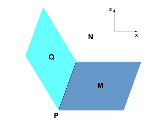
Figure 1: Geometry of AdS/BCFT

In this paper, we consider AdS/BCFT with the CBC (4).

Before we start, it is instructive to consider the simplest vacuum solution of AdS/BCFT with the bulk metric given by a part of $AdS_{d+1}$:

$$ds^{2}=dr^{2}+\cosh^{2}r\;\frac{dw^{2}+\sum_{a=1}^{d-1}dy_{a}^{2}}{w^{2}},\ \ -\rho\leq r<\infty,$$ (7)

and with the end-of-the-world brane $Q$ situated at

$$r=-\rho.$$ (8)

Here $\rho$ is a constant determined by $T=(d-1)\tanh\rho$. Note that the extrinsic curvature actually satisfies the constraint (3) and the action variation (2) vanishes automatically. As a result, the vacuum solution (7), (8) is actually a solution to AdS/BCFT independent of the type of boundary conditions imposed. In particular, it is a solution to the AdS/BCFT with NBC [39], DBC [42] as well as the CBC (4). For convenience of later use, the solution can also be written in the Poincare coordinates by performing the coordinate transformations

$$z=w/\cosh r,\ \ x=w\tanh r.$$ (9)

The metric (7) becomes

$$ds^{2}=\frac{dz^{2}+dx^{2}+\sum_{a=1}^{d-1}dy_{a}^{2}}{z^{2}}$$ (10)

and the embedding function of $Q$ becomes

$$x=-\sinh\rho\ z.$$ (11)

Some comments are in order. First, the CBC (4) apply to only the dimensions higher than two, i.e., $d>2$. That is because the 1d and 2d space are always conformal flat, so the second condition (4b) is trivial for $d\leq 2$. Second, in the above we have considered the choice of parameter $T<(d-1)$ such that the vacuum AdS can be foliated into slices with $Q$ being an AdS space (7). It is possible to consider other foliations of the AdS space such that $Q$ is a dS space or a flat space. This corresponds to the choices of the tension $T=(d-1)\coth\rho>(d-1)$ or $T=(d-1)$ respectively. In this paper, we focus on the case with AdS fiolation. The analysis performed in this paper can be easily generalized to these other cases.

2.1 Casimir effects, Weyl anomaly and displacement operator

For our purpose, let us give a quick review of the Casimir effects, Weyl anomaly and displacement operator for BCFTs. In the following sections, we will frequently use the central charges introduced in this subsection.

It is found in [55] that the renormalized stress tensor of BCFT is divergent near the boundary,

$$\langle T_{ij}\rangle=-2\alpha_{d}\frac{\bar{k}_{ij}}{x^{d-1}},\quad x\sim 0,$$ (12)

where $x$ is the proper distance from the boundary, $\bar{k}_{ij}$ are the traceless parts of extrinsic curvatures and $\alpha$ is a constant which depends only on the kind of BCFT under consideration. The coefficient $\alpha$ fixes the leading shape-dependence of Casimir effects of BCFTs.

Remarkably, the authors of [49] observe that the above Casimir coefficients are closely related to the central charges of Weyl anomaly. For example, there are universal relations

$$\alpha_{3}=b_{2},\ \ \alpha_{4}=-\frac{b_{4}}{2},$$ (13)

where $b_{i}$ are boundary central charges of Weyl anomaly of 3d BCFT and 4d BCFT [56, 57, 58, 59], respectively

$$\mathcal{A}=\int_{P}\sqrt{h}(b_{1}\mathcal{R}+b_{2}\text{Tr}\bar{k}^{2}),$$ (14)

$$\mathcal{A}=\text{Bulk Weyl anomaly}+\int_{P}\sqrt{h}(b_{3}\text{Tr}\bar{k}^{3}+b_{4}C^{ac}_{\ \ \ bc}\bar{k}_{\ a}^{b}).\;\;$$ (15)

The intimate connection of the Weyl anomaly to the Casimir effects has been generalized to higher dimensions [60], to anomalous currents [61, 62, 63, 64] and Fermion condensations [65, 66].

Due to the boundary, the energy moment tensor of BCFT is no longer conserved generally. Instead, we have [67]

$$\nabla_{i}T^{ij}=-\delta(x)D^{j}(y^{a}),$$ (16)

where $D^{j}(y^{a})$ is the displacement operator with scaling dimension $\Delta=d$. The two point function of displacement operator is given by

$$\langle D^{x}(y)D^{x}(0)\rangle=\frac{C_{D}}{|y|^{2d}},$$ (17)

with $x$ denotes the normal direction, $C_{D}$ is the Zamolodchikov norm, which is a piece of BCFT data [67]. In particular, we have

$$C_{D}\geq 0.$$ (18)

It is found in [60] that there is a universal relation

$$\alpha_{d}=\frac{d\Gamma(\frac{d+1}{2})\pi^{\frac{d-1}{2}}}{2(d-1)\Gamma(d+2)}C_{D},$$ (19)

between the Casimir coefficient (12) and displacement operator (17). See also [68, 69] where an equivalent relation is found for $d=3$ and $d=4$.

2.2 AdS/BCFT with NBC and DBC

The Casimir coefficient $\alpha_{d}$ is determined in terms of the boundary central charge. Similar to the case of the bulk Weyl anomaly [70], one can expect that generally the boundary Weyl anomaly (and hence the boundary central charges) can also be fixed holographically once the dual gravitational background is specified. This has been shown to be indeed the case in [49, 42] for 3d and 4d holographic BCFT obeying NBC and DBC respectively. Let us first briefly review this construction.

In [49, 42], the following ansatz of the bulk metric

$$ds^{2}=\frac{1}{z^{2}}\Big{[}dz^{2}+dx^{2}+\Big{(}\delta_{ab}-2\epsilon\ x\bar{k}_{ab}f(\frac{z}{x})-2\epsilon\ x\frac{k}{d-1}\delta_{ab}\Big{)}dy^{a}dy^{b}+O(\epsilon^{2})\Big{]}$$ (20)

was considered, where $k_{ab}$ is a symmetric matrix, $\bar{k}_{ab}$ its traceless part and $k$ its trace. Without loss of generality, one can choose the boundary condition

$$f(0)=1$$ (21)

at $z=0$ and the induced metric on $M$ reads [49]

$$ds_{M}^{2}=dx^{2}+\big{(}\delta_{ab}-2\epsilon xk_{ab}\big{)}dy^{a}dy^{b}+O(\epsilon^{2}).$$ (22)

Therefore $k_{ab}$ is simply the extrinsic curvature of the boundary $P$ of the BCFT. The metric (20) is considered perturbatively with small $k_{ab}$. However the dependence in $z$ is exact at each perturbative order. The function $f$ can be determined by substituting (20) into the Einstein equations. Performing a perturbative expansion in small $k_{ab}$, with $\epsilon$ counting the order of perturbations, we obtain at the order $O(\epsilon)$ a single equation

$$s\left(s^{2}+1\right)f^{\prime\prime}(s)-(d-1)f^{\prime}(s)=0.$$ (23)

This can be solved with

$$f(s)=1+\alpha_{d}\frac{s^{d}\,{}_{2}F_{1}\left(\frac{d-1}{2},\frac{d}{2};\frac{d+2}{2};-s^{2}\right)}{d},$$ (24)

where have used the BC (21) and $\alpha_{d}$ is an integration constant. From (20) and (24), we obtain the holographic stress tensor

$$T_{ij}=d\frac{\delta g_{ij}}{z^{d}}=-2\epsilon\alpha_{d}\frac{\bar{k}_{ij}}{x^{d-1}}+O(\epsilon^{2}),$$ (25)

which takes the expected form (12). According to section 2.1, the integral constant $\alpha_{d}$ is related to the Casimir coefficient (12), the central charges of Weyl anomaly (13) and the norm of displacement operator (19). So far $\alpha_{d}$ is arbitrary. This is correct as we have not specialized to any specific kind of BCFT.

To specify the holographic BCFT, the position of $Q$ needed to be constrained by imposing a BC on it. Consider an embedding of $Q$ given by

$$x=-\sinh\rho\ z+\lambda\epsilon kz^{2}+O(\epsilon^{2}).$$ (26)

As shown in [49, 42], this is a solution of the NBC or DBC if $\alpha_{d}$ and $\lambda$ are fixed to be:

$$\lambda=\frac{\cosh^{2}\rho}{2(d-1)},$$ (27)

$$\alpha_{Nd}=\frac{-d\cosh^{d}\rho}{(-\coth\rho)^{d}\,_{2}F_{1}\left(\frac{d-1}{2},\frac{d}{2};\frac{d+2}{2};-\text{csch}^{2}\rho\right)+d\cosh^{2}\rho\coth\rho},$$ (28)

$$\alpha_{Dd}=\frac{-d(-\text{csch}\rho)^{-d}}{\,{}_{2}F_{1}\left(\frac{d-1}{2},\frac{d}{2};\frac{d+2}{2};-\text{csch}^{2}\rho\right)}.$$ (29)

Note that suitable analytic continuation of the hypergeometric function should be taken in order to get smooth function at $\rho=0$ [49, 42]. For example, we have for $d=3,4$ explicitly,

$$\alpha_{N3}=\frac{2}{\pi+4\tan^{-1}\left(\tanh\left(\frac{\rho}{2}\right)\right)},\qquad\alpha_{N4}=\frac{1}{2(1+\tanh\rho)},$$ (30)

$$\alpha_{D3}=\frac{2}{\pi+4\tan^{-1}\left(\tanh\left(\frac{\rho}{2}\right)\right)+2\text{csch}\rho},\qquad\alpha_{D4}=\frac{\tanh\rho}{(1+\tanh\rho)^{2}}.$$ (31)

At this point, one can try to repeat the analysis for the CBC (4). However there is a small subtlety. We note that for $k_{ab}=0$, the unperturbed metric is just the AdS vacuum and $Q$ is an AdS-slice, which is conformally flat. As such the CBC simply asserts that the perturbed metric (20) must also be conformally flat:

$$K=\frac{3}{2}T,\quad\qquad C_{ijk}=0,\quad\mbox{for $d=3$},$$ (32a)

$$K=\frac{d}{d-1}T,\quad C^{i}{}_{jkl}=0,\quad\mbox{for $d\geq 4$},$$ (32b)

where $C_{ijk}$ and $C_{ijkl}$ are the intrinsic Cotton tensors and Weyl curvature tensors on $Q$, respectively. We have

$$C_{ijk}=2\nabla_{[i}S_{j]k},\quad C^{ij}_{\ \ kl}=R^{ij}_{\ \ kl}-4\delta^{[i}_{[k}S^{j]}_{l]},$$ (33)

where $S_{ij}$ is the Schouten tensor

$$S_{ij}=\frac{1}{d-2}\Big{(}R_{ij}-\frac{1}{2(d-1)}Rh_{ij}\Big{)}.$$ (34)

Note that $C_{ijk}$ and $C^{i}_{\ jkl}$ are Weyl invariant for $d=3$ and $d\geq 4$, respectively. It is easy to see that the CBC (32) fixes $\lambda$ to be given by the same (27). This is easy to understand since $\lambda$ is actually fixed by the asymptotic symmetry of AdS, which is universal and is independent of the BCs [2, 3]. However (32) does not fix the integral constant $\alpha_{d}$. The reason is because, as a result of (20), (26), (27), the induced metric on $Q$ is

$$ds_{Q}^{2}=\frac{\sinh^{2}\rho}{x^{2}}\Big{[}\coth^{2}\rho\;dx^{2}+\big{(}\delta_{ab}-2\epsilon\ x\bar{k}_{ab}f(-\text{csch}\rho)-2\epsilon\ x\frac{k}{d-1}\delta_{ab}\big{)}dy^{a}dy^{b}+O(\epsilon^{2})\Big{]},\;$$ (35)

and this is conformal equivalent to

$$ds_{Q}^{2}=dx^{2}+(\delta_{ab}-2\epsilon\ xK_{ab})dy^{a}dy^{b}+O(\epsilon^{2}),$$ (36)

where $K_{ab}$ are some constant tensors related to $k_{ab}$ and $f(-\text{csch}(\rho))$, whose exact expressions are not important. Now as the Cotton tensors and the Weyl tensors (33) contain three and two derivatives, respectively. As a result, for constant $K_{ab}$, we have $C_{ijk}\sim\epsilon^{3}K^{3}$ and $C_{ijkl}\sim\epsilon^{2}K^{2}$, which vanish at the linear order of $O(\epsilon)$. This means that the induced metric (35) on $Q$ is always conformal flat at the linear order $O(\epsilon)$, and the CBC (32) does not impose any constraint on the function $f(s)$. Therefore, unlike the NBC and DBC, the imposition of the CBC (32) does not fix the integral constant $\alpha_{d}$ of the bulk solution (20). This does not mean that there is any problem with the CBC. It just mean that the ansatz (20) for the bulk metric has to be more complicated in the case of CBC.

2.3 AdS/BCFT with CBC

From the discussions above, it is clear that it is the constant extrinsic curvature $k_{ab}$ that makes the induced metric on $Q$ to be trivially conformal flat at the first order of $\epsilon$. The condition (32) will become nontrivial if we consider more general extrinsic curvature $k_{ab}(y^{a})$ which depends on the coordinates on the brane $Q$. In this case, the Cotton tensors and the Weyl tensors is generically non-zero at the linear order of $O(\epsilon)$ and the nontrivial constraint provided by (32) on the bulk metric can fix the integration constant $\alpha_{d}$.

For simplicity, we focus on AdS₅/BCFT₄ with the following bulk metric

$$ds^{2}=\frac{1}{z^{2}}\Big{[}dz^{2}+dx^{2}+\delta_{ab}dy^{a}dy^{b}-4\epsilon xk_{12}(y_{3})f(\frac{z}{x})dy_{1}dy_{2}+O(\epsilon^{2})\Big{]},$$ (37)

and the embedding function of $Q$

$$x=-\sinh\rho\ z+O(\epsilon^{2}).$$ (38)

Here $k_{12}(y_{3})$ is given by

$$k_{12}(y_{3})=k^{(0)}_{12}+\kappa\ y_{3}k^{(1)}_{12}+O(\kappa^{2}),$$ (39)

where $\kappa$ is a small perturbation parameter, and $k^{(0)}_{12},k^{(1)}_{12}$ are constants. Note that the above metric is designed so that the intrinsic Weyl tensors $C_{ijkl}\sim k^{(1)}_{12}\epsilon\kappa+O(\epsilon^{2},\kappa^{2})$ are non-zero on the brane $Q$. Substituting (37) into the Einstein functions, we get the EOM of $f(s)$ as (23), which can be solved as (24). For $d=4$, we have

$$f(s)=1-2\alpha_{4}+\frac{\alpha_{4}\left(s^{2}+2\right)}{\sqrt{1+s^{2}}}.$$ (40)

From the CBC (32b), we get one independent equation at the linear order of $O(\kappa)$

$$f(-\text{csch}\rho)\ k^{(1)}_{12}\epsilon\kappa+O(\epsilon^{2},\kappa^{2})=0,$$ (41)

which imposes a non-trivial constraint on $f(s)$. From (40) and (41), the integral constant is fixed to be

$$\alpha_{C4}=\frac{\tanh\rho}{(1+\tanh\rho)^{2}},$$ (42)

where ‘C’ denotes CBC. Interestingly, $\alpha_{C4}$ is exactly the same as that of DBC (31). From (37), (40) and (25), we arrive at the holographic stress tensor

$$T_{12}=-2\epsilon\ \alpha_{C4}\frac{k_{12}(y_{3})}{x^{3}}+O(\epsilon^{2},\kappa^{2}).$$ (43)

As we reviewed in section 2.1, $\alpha_{C4}$ gives the central charge $b_{4}$ of the boundary Weyl anomaly.

We remark that the ansatz (37), (38) can be naturally generalized to higher dimensions. In fact, a more general ansatz would be

$$ds^{2}=\frac{1}{z^{2}}\Big{[}dz^{2}+dx^{2}+\big{(}\delta_{ab}-2\epsilon\ x\bar{k}^{(0)}_{ab}f(\frac{z}{x})\big{)}dy^{a}dy^{b}-2\epsilon\kappa\ xy_{a}H_{abc}(\frac{z}{x})dy^{b}dy^{c}+O(\epsilon^{2},\kappa^{2})\Big{]},$$

(44)

$$Q:x=-\sinh\rho\ z+\epsilon\kappa\ \lambda_{a}z^{2}y^{a}+O(\epsilon^{2},\kappa^{2}),$$ (45)

where $x^{i}=(x,y^{a})$, $\lambda_{a}$ and $H_{abc}(s)$ are constants and functions to be determined. For simplicity, we have set the trace $k=0$ above. However, the price to pay for the ansatz (2.3) (and also for (37)) is that they depends on too many coordinates $(z,x,y^{a})$, and this makes the analysis of the Einstein equation and the AdS/BCFT very complicated.

In this regard, it is instructive to consider the bulk solution in the coordinates system $(r,w,y_{a})$. For simplicity, let us focus on the case with vanishing traces of extrinsic curvatures, i.e, $k=0$. Applying the coordinate transformations (9), the perturbed metric (20) becomes

$$ds^{2}=dr^{2}+\cosh^{2}(r)\frac{dw^{2}+\big{(}\delta_{ab}-2\epsilon W(w)F(r)\bar{k}_{ab}\big{)}dy^{a}dy^{b}}{w^{2}}+O(\epsilon^{2}),$$ (46)

where

$$W(w)=w,$$ (47)

$$F(r)=\tanh(r)f(\text{csch}r),$$ (48)

and $f(s)$ is given by (24). The embedding function of $Q$ (26) becomes

$$r=-\rho+O(\epsilon^{2}).$$ (49)

Imposing NBC (3) and DBC (5), we get respectively

$$\text{NBC}:\ F^{\prime}(-\rho)=0,$$ (50)

$$\text{DBC}:\ F(-\rho)=0.$$ (51)

One the other hand, imposing CBC (32) we obtain

$$\text{CBC}:\begin{cases}\ W^{(3)}(w)F(-\rho)=0,&\ d=3,\\ \ W^{(2)}(w)F(-\rho)=0,&\ d\geq 4,\end{cases}$$ (52)

where $(n)$ denotes the $n$th derivative. Note that Cotton tensors (33) contain three derivatives and Weyl tensors include two derivatives, that is why we have $W^{(3)}(w)$ for $d=3$, while $W^{(2)}(w)$ for $d\geq 4$ above. Due to (47), CBC (52) is automatically satisfied and do not impose any constraint on $F(-\rho)$. As a result, one cannot fix the integral constant in $F(\rho)$ (48), or equivalently, in $f(s)$ (24).

To resolve this issue, one may consider a more general non-constant $k_{ab}$ as before. However, it is clear from (52) that the problem can also be resolved if $W^{(3)}(w)$ and $W^{(2)}(w)$ are non-zero. In fact, the choice (47) $W(w)=w$ is quite special and can be made more general. Substituting (46) together with (48, 24) into Einstein equations, we obtain the EOM of $W(w)$:

$$w^{2}W^{\prime\prime}(w)-(d-2)wW^{\prime}(w)+(d-2)W(w)=0,$$ (53)

which can be solved as

$$W(w)=\begin{cases}\ w(1+\kappa\log w),&\ d=3,\\ \ w(1+\kappa\ w^{d-3}),&\ d\geq 4,\end{cases}$$ (54)

where $\kappa$ is an arbitrary constant. For non-zero $\kappa$, $W^{(3)}(w)$ and $W^{(2)}(w)$ are indeed non-vanishing. As a result, from (52) we obtain

$$\text{CBC}:F(-\rho)=0,$$ (55)

which is exactly the same as DBC (51). This is not surprising. After all, keeping the induced metrics invariant (DBC) is a special case which keeps the induced metrics conformal invariant (CBC). However it should be stressed that, in general, CBC and DBC are different. As a result, the CBC (55) fixes the integral constant to be the same as the one (29) of DBC.

Some comments are in order. 1. For general $W(w)$, CBC is well-defined and yields the same integral constants/central charges (29) as DBC. 2. Although CBC and DBC have the same $\alpha_{d}$ central charge, as we will show in the section 4, the locations of end-of-the-world brane $Q$ are different for the two BCs and they define different holographic BCFT in general. 3. For the general $W(w)$ of (54), the induced metric on the AdS boundary $M$ ($z=w/\cosh r=0$) becomes

$$ds_{M}^{2}=dx^{2}+\Big{(}\delta_{ab}-2\epsilon(x+\kappa\ x^{d-2})k_{ab}\Big{)}dy^{a}dy^{b}+O(\epsilon^{2}),$$ (56)

where $x^{d-2}$ should be understood as $x\log x$ for $d=3$ and we have used $F(\infty)=f(0)=1$ from (48,21). For $d>3$, it is clear from (56) that $\kappa$ does not affect the value of extrinsic curvatures

$$\hat{k}_{ab}=-\frac{1}{2}\partial_{x}g_{ab}|_{x=0}=k_{ab}.$$ (57)

While for $d=3$, we have

$$\hat{k}_{ab}=-\frac{1}{2}\partial_{x}g_{ab}|_{x=0}=(1+\kappa\log x)k_{ab}|_{x=0},$$ (58)

which seems to be ill-defined unless $\kappa=0$. Note that we have the freedom to Weyl rescale the metric for a BCFT

$$ds_{M}^{2}\sim G^{2}(x)\Big{(}dx^{2}+\Big{(}\delta_{ab}-2\epsilon(x+\kappa\ x\log x)k_{ab}\Big{)}dy^{a}dy^{b}\Big{)}+O(\epsilon^{2}).$$ (59)

For $G(x)=1/(1+\kappa\log x)$, one can indeed get a well-defined extrinsic curvature.

$$\hat{k}_{ab}=\lim_{x\to 0}\frac{1}{G(x)}\partial_{x}\Big{[}G(x)^{2}(x+\kappa\ x\log x)\Big{]}=k_{ab}.$$ (60)

In fact, a simpler way to get a well-defined extrinsic curvature is to take $\kappa$ as a regularization parameter. We take $\kappa$ small but finite at the beginning and set it to zero at the end of calculations. Another regularization is that we focus on the case $d>3$ and derive the central charges by performing the analytical continuation $d\to 3$ at the end. From (29), it is clear that the analytical continuation $d\to 3$ is well-defined. 4. For more general background metrics such as black strings, the natural BC on the horizon yields $\kappa\neq 0$ and thus the well-defined CBC (55) is obtained without any arbitrariness. Please see the next section for details.

3 AdS/BCFT with CBC in more general background

In the above section, we have focused on the perturbations around a vacuum AdS background with $Q$ being a AdS space. In this section, we study holographic BCFT with CBC in more general backgrounds with $Q$ given by a deformation of the AdS black hole. In general, the induced metric on $Q$ is no longer conformally flat and the CBC (32) should be replaced by

$$K=\frac{3}{2}T,\quad\qquad\delta C_{ijk}=0,\quad\mbox{for $d=3$},$$ (61a)

$$K=\frac{d}{d-1}T,\quad\delta C^{i}_{\ jkl}=0,\quad\mbox{for $d\geq 4$},$$ (61b)

since a conformal rescaling of the metric does not affect the Cotton tensor and the Weyl tensor. A more covariant expression is that we keep conformally invariant all of the scalars constructed from the intrinsic Cotton tensors and Weyl tensors on $Q$. For example, we have $\delta(|g|C_{ijl}C^{ijk})=0$ for $d=3$, $\delta(|g|^{2/d}C_{ijkl}C^{ijkl})=0$ for $d\geq 4$ and so on.

Since CBC take different forms for $d=3$ and $d>3$, we discuss them separately below. The main purpose of this section is to show that, in the general background, CBC is well-defined and can determine all of the integral constants and thus the central charges of the Weyl anomaly.

3.1 3d BCFT

Let us start with the case $d=3$ and consider the following ansatz

$$ds^{2}=dr^{2}+\frac{\cosh^{2}(r)}{w^{2}}\Big{[}\frac{dw^{2}}{1-{w^{2}}/{w_{h}^{2}}}-(1-{w^{2}}/{w_{h}^{2}})dt^{2}+dy^{2}$$

$$\ \ \ \ \ \ \ \ \ \ \ \ \ \ \ \ \ \ \ \ \ \ \ \ \ \ \ \ \ \ \ -4\epsilon k_{ty}(1-{w^{2}}/{w_{h}^{2}})W(w)F(r)dtdy\Big{]}+O(\epsilon^{2}),$$

$$Q:\ r=-\rho+O(\epsilon^{2}),$$ (62)

where $k_{ty}$ is the extrinsic curvature and $w_{h}$ denotes the location of horizon. Note that the induced background geometry on $Q$ is a BTZ black hole. Substituting (3.1) into Einstein equations and separating variables, we get

$$\frac{F^{\prime\prime}(r)+3\tanh(r)F^{\prime}(r)}{F(r)\text{sech}^{2}(r)}=\gamma,$$ (64)

$$\frac{w\left(w\left(w^{2}-w_{h}^{2}\right)W^{\prime\prime}(w)+\left(w_{h}^{2}+3w^{2}\right)W^{\prime}(w)\right)}{w_{h}^{2}W(w)}=\gamma,$$

where $\gamma$ is the constant of separation. In general, $\gamma$ can have non-trivial dependence on $w_{h}$. Physically we require that the induced metric on the AdS boundary is given by (22) in the large $w_{h}$ limit. As the LHS of the EOM of $F(r)$ is independent of $w_{h}$, the simplest solution is obtained if $\gamma$ is independent of $w_{h}$, i.e.

$$\gamma=1.$$ (65)

More general solutions are possible as long as $\gamma=1$ in the limit of large $w_{h}$. We will focus on the choice (65) here, where in this case $F$ is given by (48) as in section 2.3 before and the equation (64) has the solution

$$W(w)=c_{1}G_{2,2}^{2,0}\left(\frac{w^{2}}{w_{h}^{2}}|\begin{array}[]{c}0,1\\ \frac{1}{2},\frac{1}{2}\\ \end{array}\right)+c_{2}\frac{wE\left(\frac{w^{2}}{w_{h}^{2}}\right)}{w^{2}-w_{h}^{2}},$$ (68)

where $G_{2,2}^{2,0}$ is Meijer $G$ function and $E$ denotes the complete elliptic integral. Recall that there is a BTZ black hole on the brane $Q$. We impose the natural BC on the black hole horizon

$$W(w_{h})\ \text{is finite},$$ (69)

which yields

$$c_{2}=0.$$ (70)

Expanding (68) around $w=0$, we have

$$W(w)=c_{1}w\frac{1+\log w-\log 4w_{h}}{\pi w_{h}}+O(w^{2}).$$ (71)

Comparing with (54), we get

$$c_{1}=\frac{\pi w_{h}}{1-\log 4w_{h}},\quad\kappa=\frac{1}{1-\log 4w_{h}}.$$ (72)

Thus the natural BC on the horizon yields a non-zero $\kappa$. As we have discussed in section 2.3, the non-zero $\kappa$ yields a well-defined CBC.

Now imposing the CBC (61) on $Q:r=-\rho$, we get two independent equations:

$$\frac{w\left(w^{2}-w_{h}^{2}\right)W^{\prime\prime}(w)+\left(w_{h}^{2}+3w^{2}\right)W^{\prime}(w)}{w_{h}^{4}}F(-\rho)=0,$$ (73)

$$\frac{\left(9w^{2}-5w_{h}^{2}\right)W^{\prime}(w)+\left(w^{2}-w_{h}^{2}\right)\left(\left(w^{2}-w_{h}^{2}\right)W^{(3)}(w)+7wW^{\prime\prime}(w)\right)}{w_{h}^{4}}F(-\rho)=0,$$ (74)

which reduce to (52) in the large $w_{h}$ limit. Substituting $W(w)$ (68) with $c_{2}=0$ into the above equations, we find that the coefficients of $F(-\rho)$ are non-zero. As a result, (73) and (74) are satisfied if $F(-\rho)=0$. This is precisely the same as (55) before and give rises to a well-defined CBC which fixes all of the integral constants and the central charges of the Weyl anomaly.

Some comments are in order. 1. EOM, BCs and solutions of $F(r)$ are the same for the AdS background (46) and the more general background (3.1). As a result, the integral constants (central charges) $\alpha_{d}$ are given by the same (29) for these two backgrounds. This is consistent with the fact that holographic boundary central charges are independent of the bulk solutions. 2. Recall that from (72) we have $\kappa\to 0$ in the limit $w_{h}\to\infty$. The metric (3.1) considered in this section provides an exact realization of the regularization discussed around (58) of section 2.3. We can first consider the metric (3.1) with a large but finite $w_{h}$, which yield a well-defined CBC (55) and fix the integral constants. Then we set $w_{h}\to\infty$ and thus $\kappa\to 0$, which give a well-defined extrinsic curvature (58). 3. Finally, we remark that for the general metric (3.1) with finite $w_{h}$, the induced spacetime on the AdS boundary $M$ is not flat.

3.2 4d BCFT

Let us go on to discuss the case $d\geq 4$. For simplicity, we focus on $d=4$ in this subsection and the generalization to higher dimensions is straightforward. We take the following ansatz

$$ds^{2}=dr^{2}+\frac{\cosh^{2}(r)}{w^{2}}\Big{[}\frac{dw^{2}}{1-{w^{3}}/{w_{h}^{3}}}-(1-{w^{3}}/{w_{h}^{3}})dt^{2}+dy_{1}^{2}+dy_{2}^{2}$$

$$\ \ \ \ \ \ \ \ \ \ \ \ \ \ \ \ \ \ \ \ \ \ \ \ \ \ \ \ \ \ \ -4\epsilon k_{12}W(w)F(r)dy_{1}dy_{2}\Big{]}+O(\epsilon^{2})$$ (75)

$$Q:\ r=-\rho+O(\epsilon^{2}),$$ (76)

where $k_{12}$ denotes the extrinsic curvature and the first line of (3.2) is the metric of a black string. Substituting (3.2) into the Einstein equations and separate the variables as before, we obtain

$$\frac{F^{\prime\prime}(r)+4\tanh(r)F^{\prime}(r)}{F(r)\text{sech}^{2}(r)}=\gamma,$$ (77)

$$\frac{w\left(w\left(w^{3}-w_{h}^{3}\right)W^{\prime\prime}(w)+\left(2w_{h}^{3}+w^{3}\right)W^{\prime}(w)\right)}{w_{h}^{3}W(w)}=\gamma,$$ (78)

where $\gamma$ is a constant. Similar to the case of 3d BCFT, a simple solution where $F(r)$ is independent of $w_{h}$ is obtained if

$$\gamma=2.$$ (79)

In this case $F(r)$ is given by (48), (24) as in section 2.

Solving (78) with $\gamma=2$, we get

$$W(w)=c_{1}w\,_{2}F_{1}\left(\frac{1}{3},\frac{1}{3};\frac{2}{3};\frac{w^{3}}{w_{h}^{3}}\right)+c_{2}w^{2}\,_{2}F_{1}\left(\frac{2}{3},\frac{2}{3};\frac{4}{3};\frac{w^{3}}{w_{h}^{3}}\right),$$ (80)

Imposing the natural BC (69) on the black hole horizon $w=w_{h}$, we obtain

$$c_{2}=-\frac{\Gamma\left(\frac{2}{3}\right)^{3}}{\Gamma\left(\frac{1}{3}\right)^{2}\Gamma\left(\frac{4}{3}\right)w_{h}}c_{1}.$$ (81)

Expanding (80) with (81) around $w=0$, we have

$$W(w)=c_{1}w-\frac{c_{1}w^{2}\Gamma\left(\frac{2}{3}\right)^{3}}{w_{h}\Gamma\left(\frac{1}{3}\right)^{2}\Gamma\left(\frac{4}{3}\right)}+O\left(w^{3}\right)$$ (82)

and hence

$$c_{1}=1,\quad\kappa=\frac{-\Gamma\left(\frac{2}{3}\right)^{3}}{w_{h}\Gamma\left(\frac{1}{3}\right)^{2}\Gamma\left(\frac{4}{3}\right)}$$ (83)

when (82) is matched with (54). Similar to the 3d case, the natural BC on the horizon yields a non-zero $\kappa$, and $\kappa$ vanishes in the large $w_{h}$ limit. Note that the BC (54) is chosen for $W(w)$ so that the induced metric on the AdS boundary is given by (56), which makes $k_{12}$ of (3.2) to be really an extrinsic curvature.

Now imposing the CBC (61) on the end-of-the-world brane $Q$, we get two independent equations

$$\frac{wW(w)}{w_{h}^{3}}F(-\rho)=0,$$ (84)

$$W^{\prime\prime}(w)F(-\rho)=0,$$ (85)

which agree with (52) in the large $w_{h}$ limit. From (80), (81), it is clear that $W(w)$ and $W^{\prime\prime}(w)$ are non-zero. As a result, (84) yields $F(-\rho)=0$, which is the same (55) as before. It gives a well defined CBC and fixes all the integral constants (central charges) in $F(r)$.

To summarize, we have shown in this section that the more general metrics (3.1), (3.2) yield a well-defined CBC without any arbitrariness. In the large horizon limit $w_{h}\to\infty$, we have $\kappa\to 0$. In this sense we can think of the metrics (3.1), (3.2) as ones providing an explicit regularization discussed in section 2.3: that we first take $w_{h}$ large but finite to get a well-defined CBC, and then send $w_{h}\to\infty$ to have a well-defined extrinsic curvature. Since the central charges are independent of $w_{h}$ and $\kappa$, the regularization of section 2.3 is well-defined.

4 AdS/BCFT with CBC up to the 2nd order of perturbations

In the previous sections, we have focused on the linear perturbations in the extrinsic curvature around an AdS background and a black string background. At this order, the coefficient $\alpha_{d}$ (and hence the bulk background) as well as the location of $Q$ are found to be the same for CBC and DBC. To detect and determine the other central charges of the theory, analysis beyond the linear perturbation is needed.

In this section, we will analysis the AdS/BCFT up to the second order of perturbations. Since all of the central charges of 3d BCFTs have already been obtained through the inclusion of linear perturbations , we will focus on 4d BCFTs in this section. We will derive the B-type boundary central charges $b_{3}$ and $b_{4}$, and find that they are the same for CBC and DBC. Although the central charges are the same, the embedding functions of $Q$ are different for CBC and DBC. The calculations of this section are quite complicated. Readers who are not interested in the details can skip this section. The main results of this section are summarized in table 1 and table 2.

At the second order of perturbations, we find that it is more convenient to work with the Poincare coordinates $(z,x,y_{a})$ as it is easier to solve Einstein equations in these coordinates. Consider the following ansatz for the metric

$$ds^{2}=\frac{1}{z^{2}}\Big{[}dz^{2}+\left(1+\epsilon^{2}x^{2}\left(X(\frac{z}{x})+\kappa x\hat{X}(\frac{z}{x})\right)\right)dx^{2}$$

$$+\left(\delta_{ab}-2\epsilon\ x\left(1+\kappa\sqrt{x^{2}+z^{2}}\right)\bar{k}_{ab}f(\frac{z}{x})+\epsilon^{2}x^{2}\left(Q_{ab}(\frac{z}{x})+\kappa x\hat{Q}_{ab}(\frac{z}{x})\right)\right)dy^{a}dy^{b}\Big{]}$$

$$+O(\epsilon^{3},\kappa^{2}),$$ (86)

and for the embedding function of $Q$

$$x=-\sinh\rho\ z+\epsilon^{2}z^{3}(d_{1}+\kappa z\ d_{2})+O(\epsilon^{3},\kappa^{2}).$$ (87)

Here $d_{1}$, $d_{2}$ are constants and $X(s)$, $\hat{X}(s)$, $f(s)$, $Q_{ab}(s)$, $\hat{Q}_{ab}(s)$ are functions to be determined, $\epsilon$ is a small perturbation parameters denoting the order of the small extrinsic curvature $k_{ab}$, and we have assumed, for simplicity, that the trace of extrinsic curvature vanishes $k=0$. Similar to what we have seen in section 2.3, we have introduced a small parameter $\kappa$ whose purpose is to complicate the ansatz (4) sufficiently enough to make the CBC nontrivial so that it can be used to fix all of the integral constants in the solution. $\kappa$ is free and it can be considered as a regularization parameter since it can be set to zero at the end of the calculations and (4) (87) still solve the Einstein equation and the CBC. We remark that (4) reduces to the ansatz of [49] when $\kappa=0$. The arrival at this form of the ansatz (4), (87) with a non-zero $\kappa$ has been a nontrivial task for this part of our work.

We choose the following BCs on the AdS boundary $M$ $(z=0)$

$$f(0)=1,\quad X(0)=\hat{X}(0)=\hat{Q}_{ab}(0)=0,\quad Q_{ab}(0)=q_{ab},$$ (88)

so that the induced metric on $M$ becomes

$$ds_{M}^{2}=dx^{2}+\Big{(}\delta_{ab}-2\epsilon x(1+\kappa x)\bar{k}_{ab}+\epsilon^{2}x^{2}q_{ab}+\cdots\Big{)}dy^{a}dy^{b},$$ (89)

which reduces to the standard form of [49] when $\kappa=0$. For simplicity, we further set

$$\bar{k}_{ab}=\text{diag}(k_{1},-k_{1},0),\ \ \ \ \ \ \ \ \ \ \ \ \ q_{ab}=\text{diag}(0,0,0),$$ (90)

$$Q_{ab}(s)=\text{diag}(Q_{1}(s),Q_{2}(s),Q_{3}(s)),\quad\hat{Q}_{ab}(s)=\text{diag}(\hat{Q}_{1}(s),\hat{Q}_{2}(s),\hat{Q}_{3}(s)).$$ (91)

With these, one can go on to solve Einstein equations with the DBC (88) on the AdS boundary $M$ and the CBC (4) on the end-of-the world brane $Q$. The approach is similar to that of [49], so we do not repeat it here. Please see the appendix for the solutions of $f(s),X(s),\hat{X}(s),Q_{ab}(s),\hat{Q}_{ab}(s)$ and $d_{1},d_{2}$. Interestingly, we find that $f(s),X(s),Q_{ab}(s)$ are the same for CBC and DBC, while the parameter $d_{1}$ of the embedding function is different. The difference is given by

$$d_{1\ DBC}-d_{1\ CBC}=\frac{1}{18}k_{1}^{2}e^{-4\rho}\cosh\rho\coth\rho,$$ (92)

which shows that CBC and DBC are indeed different BCs. We remark that DBC (5) can fix all of the integral constants even for $\kappa=0$ [42], and so we can simply set $\kappa=0$ and do not need to care about $\hat{X}(s),\hat{Q}_{ab}(s),d_{2}$ in this case.

Substituting the metric (4) into the holographic stress tensor (25) and taking the limit $\kappa\to 0$, we obtain

$$T_{xx}=-\frac{2\epsilon^{2}k_{1}^{2}\tanh\rho}{x^{2}(1+\tanh\rho)^{2}},$$ (93)

$$T_{11}=\frac{-2\epsilon k_{1}\tanh\rho}{x^{3}(\tanh\rho+1)^{2}}+\frac{\epsilon^{2}k_{1}^{2}\text{sech}^{8}\rho(7\sinh 2\rho+\cosh 2\rho)(\sinh 6\rho+\cosh 6\rho)}{3x^{2}(\tanh\rho+1)^{8}},$$

(94)

$$T_{22}=\frac{2\epsilon k_{1}\tanh\rho}{x^{3}(\tanh\rho+1)^{2}}+\frac{\epsilon^{2}k_{1}^{2}\text{sech}^{8}\rho(7\sinh 2\rho+\cosh 2\rho)(\sinh 6\rho+\cosh 6\rho)}{3x^{2}(\tanh\rho+1)^{8}},$$

(95)

$$T_{33}=-\frac{\epsilon^{2}k_{1}^{2}\text{sech}^{8}\rho(2\cosh 2\rho-\sinh 2\rho)(\sinh 6\rho+\cosh 6\rho)}{3x^{2}(\tanh\rho+1)^{8}},$$ (96)

plus terms of $O\left(\epsilon^{3}\right)$. According to [49], the stress tensors near the boundary can be completely fixed by Weyl anomaly. Applying (A.24) and (A.26) of [49], we have

$$T_{ij}=b_{4}\frac{\bar{k}_{ij}-2x\epsilon k^{l}_{(i}\bar{k}_{j)l}}{x^{3}}\epsilon+b_{4}\frac{(n_{i}n_{j}-\frac{1}{3}h_{ij})\text{Tr}\bar{k}^{2}}{2x^{2}}\epsilon^{2}+(-3b_{3}-2b_{4})\frac{k^{l}_{(i}k_{j)l}-\frac{1}{3}h_{ij}\text{Tr}k^{2}}{x^{2}}\epsilon^{2}$$ (97)

where $b_{3},b_{4}$ are central charges of the Weyl anomaly, $n_{i}=(1,0,0,0)$, $h_{ij}=\text{diag}(0,1,1,1)$ is the boundary metric, $k_{ij}=\bar{k}_{ij}=\text{diag}(0,k_{1},-k_{1},0)$ and we have used $k=C_{ixjx}=0$ above. Comparing (97) with (93-96), we finally derive the boundary central charges for 4d BCFTs

$$b_{3}=\frac{1}{6}-\frac{e^{-4\rho}}{2},\quad b_{4}=-\frac{2\tanh\rho}{(1+\tanh\rho)^{2}}.$$ (98)

Some comments are in order. 1. To compare (97) with (93)-(96), we have two free parameters $(b_{3},b_{4})$ but four equations. It is non-trivial to have the consistent solution (98). This can be regarded as a check of our calculations. 2. Since CBC and DBC have the same bulk solutions, they have the same central charges (98) too. 3. Let us stress again that CBC and DBC have different embedding functions of $Q$ (87), (92). Thus they are different BCs. 4. To end this section, we list the central charges of the Weyl anomaly (14), (15) for various BCs in the following table 1 and table 2.

Table 1: Boundary Central Charge of 3d BCFT

charge	NBC	DBC	CBC
$b_{1}$	$\sinh\rho$	$\sinh\rho$	$\sinh\rho$
$b_{2}$	$\frac{2}{\pi+4\tan^{-1}\left(\tanh\left(\frac{\rho}{2}\right)\right)},$	$\frac{2}{\pi+4\tan^{-1}\left(\tanh\left(\frac{\rho}{2}\right)\right)+2\text{csch}\rho}$	$\frac{2}{\pi+4\tan^{-1}\left(\tanh\left(\frac{\rho}{2}\right)\right)+2\text{csch}\rho}$

Table 2: Boundary Central Charge of 4d BCFT

charge	NBC	DBC	CBC
$b_{3}$	$\frac{1}{1+\tanh\rho}-\frac{1}{3}$	$\frac{1}{6}-\frac{e^{-4\rho}}{2}$	$\frac{1}{6}-\frac{e^{-4\rho}}{2}$
$b_{4}$	$\frac{-1}{1+\tanh\rho}$	$\frac{-2\tanh\rho}{(1+\tanh\rho)^{2}}$	$\frac{-2\tanh\rho}{(1+\tanh\rho)^{2}}$

5 Metric perturbations for different BCs

According to [35], CBC is elliptic and leads to a well-defined perturbation theory for gravity. In this section, we analysis the metric perturbation with CBC, DBC and NBC imposed respectively on the end-of-the-world brane $Q$.

5.1 Metric perturbations

Consider the following ansatz of the perturbation metric and the embedding function of $Q$

$$ds^{2}=dr^{2}+\cosh^{2}r\left(\bar{h}^{(0)}_{ij}(y)+\epsilon H(r)\bar{h}^{(1)}_{ij}(y)\right)dy^{i}dy^{j}+O(\epsilon^{2}),$$ (99)

$$Q:\ r=-\rho+O(\epsilon^{2}),$$ (100)

where $\bar{h}^{(0)}_{ij}(y)$ is the unperturbed metric and $\bar{h}^{(1)}_{ij}(y)$ denotes the perturbation. Our results below for the spectrum of gravitons is independent of the choice of the unperturbed metric. Interesting examples of the unperturbed metric includes, for example, the $d$ dimensional AdS space in the RS brane world scenario or the AdS black hole for applications in islands. In terms of bulk metric perturbations, we have

$$\delta g_{r\mu}=0,\quad\delta g_{ij}=\cosh^{2}(r)H(r)\bar{h}^{(1)}_{ij}(y).$$ (101)

The usual transverse traceless gauge

$$\nabla^{\mu}\delta g_{\mu\nu}=0,\quad g^{\mu\nu}\delta g_{\mu\nu}=0,$$ (102)

reads in the linear order

$$D^{i}\bar{h}^{(1)}_{ij}=0,\quad\bar{h}^{(0)ij}\bar{h}^{(1)}_{ij}=0,$$ (103)

where $\nabla^{\mu}$ and $D^{i}$ are the covariant derivatives with respect to $g_{\mu\nu}$ and $\bar{h}^{(0)}_{ij}$ respectively. In the gauge (102), the linearlized Einstein equations become

$$\left(\nabla_{\alpha}\nabla^{\alpha}+2\right)\delta g_{\mu\nu}=0.$$ (104)

Substituting (101), (103), into (104) and separating variables, we obtain

$$\left(D_{i}D^{i}+2-m^{2}\right)\bar{h}^{(1)}_{ij}(y)=0,$$ (105)

$$\cosh^{2}(r)H^{\prime\prime}(r)+d\sinh(r)\cosh(r)H^{\prime}(r)+m^{2}H(r)=0,$$ (106)

where $m^{2}$ is the constant of separation. The spectrum of fluctuations is determined once the boundary conditions of the AdS/BCFT are specified. We impose the standard DBC on the AdS boundary $M$

$$H(\infty)=0.$$ (107)

In addition, we impose a BC on $Q$. For the choice of CBC, the second condition of (32) or the second condition (61) both yields

$$\text{CBC/DBC}:\quad H(-\rho)=0.$$ (108)

Note that DBC also yields the same condition (108). This implies that the spectrum of fluctuations are the same for CBC and DBC. As for NBC, we have the condition

$$\text{NBC}:\quad H^{\prime}(-\rho)=0.$$ (109)

Each mode of fluctuation of $\bar{h}^{(1)}_{ij}$ represents a massive graviton of mass $m$ in the theory. It also has the interpretation as fluctuation mode

$$\delta K_{ij}=-\frac{\epsilon}{2}\cosh^{2}(\rho)H^{\prime}(-\rho)\bar{h}^{(1)}_{ij}$$ (110)

of the extrinsic curvature $K_{ij}=-\frac{1}{2}\partial_{r}g_{ij}\big{|}_{r=-\rho}$ of $Q$. Note that $\delta K_{ij}$ vanishes for NBC but is non-trivial for CBC and DBC. Note also that the perturbation (110), while nontrivial, actually keeps $K$ invariant and this is consistent with the CBC and DBC.

5.2 Mass spectrum

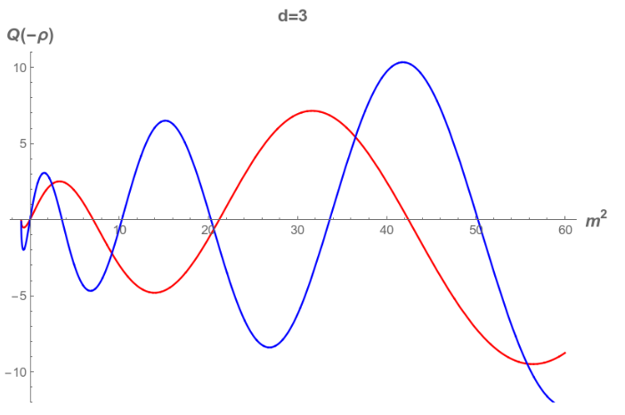
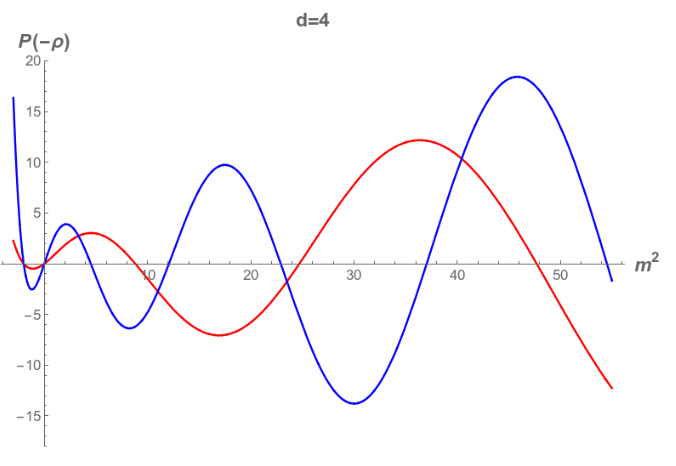
Figure 2: Mass spectrum for CBC/DBC with $d=3,4.$ Here the roots of $H(-\rho)=0$ gives the allowed masses $m^{2}$ for CBC and DBC. Red (Blue) curve is for $\rho=0.1(1)$.

Let us now work out the mass spectrum of the gravitons. For generic $m^{2}$, the general solution to (106) is given in terms of the two independent Legendre functions $P_{\lambda}^{\frac{d}{2}}(x)$ and $Q_{\lambda}^{\frac{d}{2}}(x)$ by

$$H(r)=\text{sech}^{\frac{d}{2}}(r)\left(c_{1}P_{\lambda}^{\frac{d}{2}}(\tanh r)+c_{2}Q_{\lambda}^{\frac{d}{2}}(\tanh r)\right).$$ (111)

Here $c_{1}$ and $c_{2}$ are integral constants and $\lambda$ is

$$\lambda:=\frac{1}{2}\left(\sqrt{(d-1)^{2}+4m^{2}}-1\right).$$ (112)

We note however that for the special value of $m^{2}$

$$m^{2}=\begin{cases}-\frac{1}{4}((d-1)^{2}-1),&\ \text{even $d$},\\ -\frac{1}{4}(d-1)^{2},&\ \text{odd $d$},\end{cases}$$ (113)

which corresponds to $\lambda=0$ ($d$ even) and $\lambda=-1/2$ ($d$ odd) respectively, (111) no longer gives the general solution since the Legendre functions $P^{n}_{0}(x),Q^{n+\frac{1}{2}}_{-\frac{1}{2}}(x)$ vanish identically for integer $n$. In this case, the general solution is given, for even $d$, by

$$H(r)=\text{sech}^{\frac{d}{2}}(r)\left(c_{1}e^{\frac{dr}{2}}+c_{2}e^{-\frac{dr}{2}}\right),$$ (114)

and for odd $d$, by

$$H(r)=\text{sech}^{\frac{d}{2}}(r)\left(c_{1}P^{\frac{d}{2}}_{-\frac{1}{2}}(\tanh r)+c_{2}P^{-\frac{d}{2}}_{-\frac{1}{2}}(\tanh r)\right).$$ (115)

As $P^{\pm\frac{d}{2}}_{-\frac{1}{2}}(\tanh r)\sim e^{\pm\frac{dr}{2}}$ for large $r\to\infty$, it is clear that (114,115) cannot satisfy the boundary conditions (107, 108) or (107, 109) and so we can rule out (113) from the spectrum. Next us now get back to the discussion for generic $m^{2}$. The imposition of (107) gives

$$H(r)=\begin{cases}\ c_{1}\ \text{sech}^{\frac{d}{2}}(r)\ P_{\lambda}^{\frac{d}{2}}(\tanh r),&\ \text{even $d$},\\ \ c_{2}\ \text{sech}^{\frac{d}{2}}(r)\ Q_{\lambda}^{\frac{d}{2}}(\tanh r),&\ \text{odd $d$}.\end{cases}$$ (116)

We note that for $m^{2}=0$, it is $\lambda=d/2-1$ and $H(r)$ as given by (116) is identically zero. So massless graviton is excluded for all cases, CBC, DBC and NBC, of boundary condition.

Next, let us first consider the boundary condition CBC/DBC (108) on the end-of-the-world brane $Q$. We get the constraint on $m^{2}$:

$$0=\begin{cases}P_{\lambda}^{\frac{d}{2}}\left(\tanh\left(-\rho\right)\right),&\ \text{even $d$},\\ Q_{\lambda}^{\frac{d}{2}}\left(\tanh\left(-\rho\right)\right),&\ \text{odd $d$}.\end{cases}$$ (117)

For $m^{2}<-\frac{(d-1)^{2}}{4}$ outside the Breitenlohner-Freedman (BF) bound, there is no solution to (117) since in this case $\lambda=-1/2+i\alpha\;(\alpha>0)$ becomes complex and the Legendre function $P^{\frac{d}{2}}_{\lambda}(\tanh(-\rho))$ is real and strictly positive, while $Q^{\frac{d}{2}}_{\lambda}(\tanh(-\rho))$ is purely imaginary and strictly negative for this range of $m^{2}$. For $m^{2}\geq-\frac{(d-1)^{2}}{4}$ satisfying the BF bound of AdS_d, as massless graviton is excluded, all the solutions have positive $m^{2}$. In Fig 2, we plot for $d=3,4$ the value of $P^{\frac{d}{2}}_{\lambda}(-\rho)$ or $Q^{\frac{d}{2}}_{\lambda}(-\rho)$ against $m^{2}$. The roots of the curves give the admissible values of $m^{2}$.

To get further understandings of the spectrum, let us study some special cases. For large $\rho\to\infty$, (117) can be approximated by [71]

$$0=\lim_{\rho\to\infty}H(-\rho)\sim\begin{cases}-2^{d/2}\pi^{-1}\sin(\lambda\pi)\,&\ \text{even $d$},\\ -2^{(d/2)-1}\Gamma(d/2)\cos(\lambda\pi),&\ \text{odd $d$},\end{cases}$$ (118)

which has the roots

$$m^{2}\approx k(k+d-1),\,\ \ \ \ \text{for large }\rho,$$ (119)

where $k\geq 1$ are integers. On the other hand, in the limit of small $\rho\to 0$, we have

$$0=\lim_{\rho\to 0}H(-\rho)\sim\begin{cases}f_{1}(m^{2})1/\Gamma\left(\frac{1}{4}\left(d+3-\sqrt{(d-1)^{2}+4m^{2}}\right)\right),\,&\ \text{even $d$},\\ f_{2}(m^{2})\sin\left(\frac{1}{4}\pi\left(d-1+\sqrt{(d-1)^{2}+4m^{2}}\right)\right),&\ \text{odd $d$},\end{cases}$$ (120)

where $f_{1}>0$ and $f_{2}>0$ are some unimportant positive functions. From (120), we derive the roots

$$m^{2}\approx 2k(2k+d-1),\ \ \ \ \text{for small }\rho,$$ (121)

where $k\geq 1$ are integers. Remarkably, the spectrum (121) of small $\rho$ is included in the spectrum (119) of large $\rho$ with even mass level $k$.

Finally, let us work out the metric perturbation spectrum with the NBC (109) imposed on $Q$. After some simplification, we obtain the following constraints on $m^{2}$:

$$0=\begin{cases}P_{\lambda}^{\frac{d}{2}-1}\left(\tanh\left(-\rho\right)\right),&\ \text{even $d$},\\ Q_{\lambda}^{\frac{d}{2}-1}\left(\tanh\left(-\rho\right)\right),&\ \text{odd $d$}.\end{cases}$$ (122)

We remark that while (122) for NBC appears to be the same as (122) for CBC/DBC with $d$ replaced by $(d-2)$, this is not true since the parameter $\lambda$ as given by (112) is not changed. The analysis of the solutions to (122) is similar to the the discussion above for the case of CBC/DBC. The perturbation modes are all positive, as seen in the figure 3.

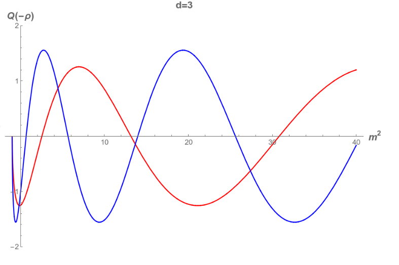
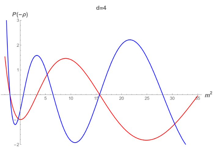
Figure 3: Mass spectrum for NBC with $d=3,4.$ Here the roots of $H^{\prime}(-\rho)=0$ gives the allowed masses $m^{2}$ for NBC. Red (Blue) curve is for $\rho=0.1(1)$.

Summarizing, the quadratic metric fluctuations of AdS/BCFT are all massive. On the end-of-the-world brane, they manifest as fluctuation modes (110) of the extrinsic curvature $\delta K_{ij}$ in the case of CBC and DBC, and as fluctuation modes of the metric $\delta g_{ij}$ in the case of NBC:

$$\begin{cases}\delta K_{ij}=-\frac{\epsilon}{2}\cosh^{2}(\rho)H^{\prime}(-\rho)\bar{h}^{(1)}_{ij}&\mbox{for CBC and DBC},\\ \delta g_{ij}=\epsilon\cosh^{2}(\rho)H(-\rho)\bar{h}^{(1)}_{ij}&\mbox{for NBC}.\end{cases}$$ (123)

The mass spectrum is determined by (117) in the case of CBC and DBC, and (122) in the case of NBC. The spectrum is countable and positive, and we can denote it as $\{m_{n}^{2}\}$ .

5.3 Two point functions in BCFT

As an application for the mass spectrum obtained above, let us consider the two point functions of operators in BCFT. For simplicity, let us discuss the case of primary operator ${\cal O}_{\Delta}$ with conformal dimension $\Delta$. We use the Gaussian normal coordinates $y^{i}=(w,\vec{y})$ on $M$ where $w$ is the coordinate in the normal direction and $\vec{y}=(y^{a})$ is the coordinates for the orthogonal slices. The two-point function in BCFT for primary operators ${\cal O}_{i}$ with dimensions $\Delta_{i}$ is generally given by

$$\langle{\cal O}_{1}(w,\vec{y}){\cal O}_{2}(w^{\prime},\vec{y}^{\prime})\rangle=\frac{f(\eta)}{(2w)^{\Delta_{1}}(2w^{\prime})^{\Delta_{2}}},$$ (124)

where $f$ is a function of the conformal invariant

$$\eta=\frac{(\vec{y}-\vec{y}^{\prime})^{2}+(w-w^{\prime})^{2}}{ww^{\prime}}.$$ (125)

It was shown in [72] that 2-point function for the same scalar operators $(\Delta_{1}=\Delta_{2}=\Delta$) can be constructed in terms of the bulk-to-bulk propagators in AdS space . The result is

$$f(\eta)=(2\Delta-d)^{2}\sum_{n}C_{n}^{2}{\cal G}_{n}(\eta),$$ (126)

where the sum $n$ is over the mass spectrum $\{m^{2}_{n}\}$ of the radial equation (106). Here the conformal block ${\cal G}_{n}$ is given by the standard bulk-to-bulk AdS_d propagator

$${\cal G}_{n}(\eta)=\frac{C_{\Delta_{n},d}}{2\Delta_{n}-(d-1)}(\eta)^{-\Delta_{n}}{}_{2}F_{1}\left(\Delta_{n},\Delta_{n}-\frac{d}{2}+1,2\Delta_{n}-d+2,-\frac{4}{\eta}\right),$$ (127)

where $C_{\Delta_{n},d}=\frac{\Gamma(\Delta_{n})}{\pi^{\frac{d-1}{2}}\Gamma(\Delta_{n}-\frac{d-1}{2})}$ and $\Delta_{n}$ is determined by $\Delta_{n}(\Delta_{n}-(d-1))=m_{n}^{2}$. The numerical factor $C_{n}$ can be extracted from the fall off

$$H_{n}(r)=C_{n}e^{-\Delta_{n}r}+O(e^{-(\Delta_{n}+2)r})$$ (128)

at large $r$. With the mass spectrum $\{m_{n}^{2}\}$ and the mode functions $H_{n}(r)$ we determine above, the 2-point function for holographic BCFT with CBC, DBC or NBC imposed is entirely fixed and one can perform a detailed study of its properties. Note that the EOM (105) and BCs (107, 108, 109) of $H_{n}(r)$ are exactly the same for the massless scalar and gravity in the bulk. Thus our above results can help to study the holographic two point function of the scalar primary operator (124). See appendix for the discussions of the mass spectrum for massive bulk scalars. It is also interesting to extend the analysis to determine the 2-point function for energy-momentum tensor in AdS/BCFT. We leave it to future works.

6 More physical discussions

In this section, we make more physical discussions concerning our results.

6.1 Relation to massive island

The authors of [13] notice that all reliable calculations of the Page curve in more than three dimensions have been performed in gravity theories with only massive gravitons. If one attempts to take the limit of zero graviton mass, any contribution from the islands disappears. In their following work [24], the authors further argue that islands might not constitute consistent entanglement wedges in massless gravity where the Gauss law applies. On the other hand, the puzzle can be resolved naturally in massive gravity, where the Gauss law does not apply. This implies that consistent island formation seems to be possible only in massive gravity. Their argument is general. So far islands has been studied mainly with NBC. Our results show that the gravitons in the AdS black hole backgrounds with AdS brane are indeed massive for all three kinds of boundary conditions. It will be interesting to study the properties of islands with CBC/DBC as well.

6.2 Consistency of AdS/BCFT boundary conditions

In this subsection, we argue that CBC/DBC and NBC all define a consistent theory of AdS/BCFT. Different holographic BCFTs self-consistently correspond to different boundary conditions. The reasons are as follows. First, there are generally more than one consistent boundary conditions that can be imposed for a theory. For examples, one can impose either DBC and NBC for scalar theory, and either the absolute boundary condition or the relative boundary condition for the Maxwell theory. It is natural that there are more than one consistent boundary conditions for AdS/BCFT as well. Second, we note that the holographic Weyl anomaly obtained with CBC, DBC and NBC not only admit the correct form in agreement with general classification, but also the corresponding boundary charges all possess the correct physical properties. Take 3d BCFT as an example. The A-type boundary central charge is listed in Table. 1,

$$b_{1}=\sinh\rho.$$ (129)

From the null energy condition on the brane, [39, 40] derive

$$\rho_{UV}\geq\rho_{IR},$$ (130)

which has a natural geometric interpretation [47]. From (11) [47] notices that the larger $\rho$ is, the closer the brane approaches to the AdS boundary (UV). Thus, large $\rho$ corresponds to the UV, while small $\rho$ corresponds to the IR. From (129) and (130), therefore the holographic g/c-theorem for the A-type boundary central charge

$$b_{1\ UV}\geq b_{1\ IR}$$ (131)

is observed. This is a strong support for the consistency of all 3 kinds of boundary conditions. As for the B-type boundary central charge, they are given by (30,31) and are different for CBC/DBC and NBC. For a unitary BCFT, the B-type boundary central charge, which is related to the norm of displacement operator, should be non-negative (see section 2.1 for more discussions)

$$\alpha_{d}\geq 0.$$ (132)

As shown in [42], this is indeed the case for all kinds of BCs, as long as the brane tension is non-negative, i.e., $\rho\geq 0$. In other word, CBC/DBC and NBC all yield “correct Weyl anomaly” with A-type boundary central charges obeying the holographic g/c-theorem and non-negative B-type boundary central charges that correspond to unitary theories. Third, graviton are massive for all kinds of BCs. This is another support for various choices of BCs. For the above reasons, we believe that the AdS/BCFT with CBC/DBC and NBC are all well-defined. To get more tests of different BCs, one can study two-point functions of stress tensor and the bootstrap constraints [77, 78, 79]. These are non-trivial problems which go beyond the main purpose of this paper. We leave them to future works.

7 Conclusions

In this paper, we have investigated the holographic BCFT with CBC. The CBC is an interesting BC of gravity, which is elliptic and leads to a well-defined perturbation theory of ‘quantum’ gravity [1]. For simplicity, we have focused on the classical gravity. We derived the massive gravitational modes for various boundary conditions imposed on the end-of-the-world brane $Q$. Compared with NBC and DBC, CBC is more subtle. For the simplest perturbations with homogeneous extrinsic curvature around the AdS background, we showed that CBC does not impose any constraint on the integral constants of the solution and the central charges of the Weyl anomaly. Nevertheless the central charges of the Weyl anomaly can be fixed holographically if one consider more general metric perturbations around an AdS or a black string background. In this way, we fix the central charges of Weyl anomaly for holographic BCFT with CBC. Interestingly, we find that the central charges are the same for CBC and DBC, although they are different BCs in general since they yield different locations of the end-of-the-world brane. We also study the gravitational perturbations for the different choices of BCs. Remarkably, we find that there are non-trivial gravitational dynamics from the extrinsic curvatures, which obeys EOM of massive gravity at the linear perturbations on a Dirichlet and conformal brane. Finally, we analysis the mass spectrum of metric perturbations and find that there is no massless mode in the theory for all kinds of boundary conditions. Our results show that it should be possible to form island in AdS/BCFT with CBC/DBC as well.

Many interesting problems are worth exploring. The existence of massive gravitons is interesting and it is expected to have interesting implications on the BCFT through holography. In this paper, we have worked out the mass spectrum of the gravitons. It is interesting to study the non-linear dynamics of the metric perturbations in order to better understand their interactions. Further study of double holography with CBC, such as wedge holography is also an interesting problem. For example, according to the results of this paper, the wedge holography with CBC yields the correct forms of Weyl anomaly. In particular, the A-type Weyl anomaly is exactly the same for wedge holography with CBC and NBC. Investigation of other aspects of the holography would be interesting. For example, how do the perturbation modes affect the quantum extreme surface and the island formula on the Dirichlet and conformal branes? We hope these interesting problems could be addressed in the near future.

Appendix A Second order perturbative solutions to AdS/BCFT with CBC

In this appendix, we solve the bulk Einstein equations for the ansatz (4) that include perturbations in the extrinsic curvature up to the second order. Solving Einstein equations together with the DBC (88) on AdS boundary $M$ and the CBC (32) on the end-of-brane $Q$, we obtain

$$f(s)=1+2a_{0}-\frac{a_{0}\left(s^{2}+2\right)}{\sqrt{s^{2}+1}},$$ (133)

$$X(s)=-\frac{k_{1}^{2}}{2}\left(2a_{0}\left(a_{0}\left(8\sqrt{s^{2}+1}+s^{2}\left(\log\left(s^{2}+1\right)-4\right)-8\right)-2s^{2}+4\sqrt{s^{2}+1}-4\right)+s^{2}\right),$$

$$Q_{1}(s) = a_{1}\left(s^{2}-2\sqrt{s^{2}+1}+2\right)-a_{0}^{2}k_{1}^{2}\log\left(s^{2}+1\right)$$ (135)

$$+\frac{k_{1}^{2}\left(a_{0}\left(-4s^{2}+8\sqrt{s^{2}+1}-8\right)-s^{2}+\sqrt{s^{2}+1}-1\right)}{\sqrt{s^{2}+1}}$$

$$+\frac{a_{0}^{2}k_{1}^{2}\left(-14s^{4}+\left(51\sqrt{s^{2}+1}-76\right)s^{2}+62\left(\sqrt{s^{2}+1}-1\right)\right)}{6\left(s^{2}+1\right)^{3/2}},$$

$$Q_{2}(s) = a_{2}\left(s^{2}-2\sqrt{s^{2}+1}+2\right)-a_{0}^{2}k_{1}^{2}\log\left(s^{2}+1\right)$$ (136)

$$+\frac{k_{1}^{2}\left(a_{0}\left(-4s^{2}+8\sqrt{s^{2}+1}-8\right)-s^{2}+\sqrt{s^{2}+1}-1\right)}{\sqrt{s^{2}+1}}$$

$$+\frac{a_{0}^{2}k_{1}^{2}\left(-14s^{4}+\left(51\sqrt{s^{2}+1}-76\right)s^{2}+62\left(\sqrt{s^{2}+1}-1\right)\right)}{6\left(s^{2}+1\right)^{3/2}},$$

$$Q_{3}(s) = \left(a_{1}+a_{2}\right)\left(-s^{2}+2\sqrt{s^{2}+1}-2\right)$$ (137)

$$+\frac{1}{2}k_{1}^{2}\left(a_{0}\left(-4s^{2}+8\sqrt{s^{2}+1}-8\right)-s^{2}+4\sqrt{s^{2}+1}-4\right)$$

$$+\frac{1}{6}a_{0}^{2}k_{1}^{2}\left(15s^{2}-20\sqrt{s^{2}+1}-\frac{1}{s^{2}+1}-6\log\left(s^{2}+1\right)+21\right),$$

$$\hat{X}(s) = \frac{4}{3}k_{1}^{2}\left(\left(\sqrt{s^{2}+1}-5\right)s^{2}+\sqrt{s^{2}+1}-1\right)$$ (138)

$$-\frac{2}{3}a_{0}^{2}k_{1}^{2}\left(\left(4\sqrt{s^{2}+1}+6\right)s^{2}-8\sqrt{s^{2}+1}-6\left(s^{2}+1\right)\log\left(s^{2}+1\right)+8\right)$$

$$+\frac{2}{3}a_{0}k_{1}^{2}\left(\left(8\sqrt{s^{2}+1}-15\right)s^{2}+8\left(\sqrt{s^{2}+1}-1\right)+3\left(s^{2}+1\right)\log\left(s^{2}+1\right)\right),\;\;\;\;\;$$

$$\hat{Q}_{1}(s) = \frac{1}{2}{\hat{a}}_{1}\left(\left(2\sqrt{s^{2}+1}-3\right)s^{2}+2\left(\sqrt{s^{2}+1}-1\right)\right)$$ (139)

$$+\frac{4}{3}k_{1}^{2}\left(-2s^{2}+3\sqrt{s^{2}+1}-3\right)$$

$$+\frac{2}{3}a_{0}k_{1}^{2}\left(-13s^{2}+24\left(\sqrt{s^{2}+1}-1\right)+\log\left(s^{2}+1\right)\right)$$

$$+\frac{2a_{0}^{2}k_{1}^{2}\left(\left(24-11\sqrt{s^{2}+1}\right)s^{2}-30\left(\sqrt{s^{2}+1}-1\right)+2\sqrt{s^{2}+1}\log\left(s^{2}+1\right)\right)}{3\sqrt{s^{2}+1}},\;\;\;\;\;\;\;$$

$$\hat{Q}_{2}(s) = \frac{1}{3}{\hat{a}}_{2}\left(\left(2\sqrt{s^{2}+1}-3\right)s^{2}+2\left(\sqrt{s^{2}+1}-1\right)\right)$$ (140)

$$+\frac{4k_{1}^{2}\left(-4s^{4}+s^{2}-5\sqrt{s^{2}+1}+5\right)}{9\sqrt{s^{2}+1}}$$

$$+\frac{2a_{0}k_{1}^{2}\left(-26s^{4}+20s^{2}-46\sqrt{s^{2}+1}+3\sqrt{s^{2}+1}\log\left(s^{2}+1\right)+46\right)}{9\sqrt{s^{2}+1}}$$

$$+\frac{4a_{0}^{2}k_{1}^{2}\left(-11s^{4}+14s^{2}-34\sqrt{s^{2}+1}+3\sqrt{s^{2}+1}\log\left(s^{2}+1\right)+34\right)}{9\sqrt{s^{2}+1}},$$

$$\hat{Q}_{3}(s) = \frac{\left(3{\hat{a}}_{1}+2{\hat{a}}_{2}\right)\left(-2s^{4}+\left(3\sqrt{s^{2}+1}-4\right)s^{2}+2\left(\sqrt{s^{2}+1}-1\right)\right)}{6\sqrt{s^{2}+1}}$$ (141)

$$+\frac{4k_{1}^{2}\left(s^{4}+\left(6\sqrt{s^{2}+1}+2\right)s^{2}-\sqrt{s^{2}+1}+1\right)}{9\sqrt{s^{2}+1}}$$

$$+\frac{2a_{0}^{2}k_{1}^{2}\left(46s^{4}+\left(56-57\sqrt{s^{2}+1}\right)s^{2}-10\left(\sqrt{s^{2}+1}-1\right)+6\sqrt{s^{2}+1}\log\left(s^{2}+1\right)\right)}{9\sqrt{s^{2}+1}}$$

$$+\frac{2a_{0}k_{1}^{2}\left(2\left(s^{2}-3\sqrt{s^{2}+1}+2\right)s^{2}-2\sqrt{s^{2}+1}+3\sqrt{s^{2}+1}\log\left(s^{2}+1\right)+2\right)}{9\sqrt{s^{2}+1}},$$

where the integral constants are given by

$$a_{0}=-\frac{\coth\rho}{(\coth\rho+1)^{2}},$$ (142)

$$a_{1}=a_{2}=\frac{1}{48}k_{1}^{2}e^{-4\rho}(-8\sinh 4\rho+\cosh 4\rho-9),$$ (143)

$${\hat{a}}_{1}=\frac{-k_{1}^{2}e^{-3\rho}(29\sinh 3\rho-54\sinh\rho+19\sinh 5\rho+12\cosh\rho+22\cosh 3\rho-2\cosh 5\rho)}{18\left(e^{2\rho}+3\right)},$$

(144)

$${\hat{a}}_{2}=\frac{k_{1}^{2}e^{-3\rho}(4\sinh\rho-4\sinh 5\rho+8\cosh\rho+3\cosh 3\rho+5\cosh 5\rho)}{2\left(e^{2\rho}+3\right)}.$$ (145)

Note that, according to [49], suitable analytical continuations should be performed for the above equations. In order to get continuous solutions around $x=0$, one should replace $\sqrt{1+s^{2}}=\sqrt{1+\frac{z^{2}}{x^{2}}}$ by $\sqrt{1+s^{2}}=\sqrt{x^{2}+z^{2}}/x$ when $s=z/x$ is substituted [49].

The parameters of embedding function (87) can be fixed by the CBC (4a),

$$d_{1} = \frac{1}{8}k_{1}^{2}e^{-4\rho}\sinh^{2}2\rho\sinh 4\rho\text{csch}\rho$$

$$-\frac{1}{96}k_{1}^{2}e^{-4\rho}\sinh\rho\left(8\cosh^{2}\rho+(\cosh 2\rho+4)\log\left(\coth^{2}\rho\right)\right)$$

$$+\frac{1}{96}k_{1}^{2}e^{-4\rho}\sinh\rho\left(4\cosh 4\rho\left(\log\left(\coth^{2}\rho\right)+5\right)+\cosh 6\rho\left(\log\left(\coth^{2}\rho\right)+12\right)\right),$$

$$d_{2} = \frac{1}{24}k_{1}^{2}e^{-4\rho}(-5\cosh 2\rho+7\cosh 4\rho-3\cosh(6\rho)+2)$$

$$\frac{1}{96}k_{1}^{2}e^{-4\rho}\sinh 4\rho\left(28-3\sinh^{2}2\rho\log\left(\coth^{2}\rho\right)\right)$$

$$-\frac{1}{96}k_{1}^{2}e^{-4\rho}(33\sinh 2\rho+9\sinh 6\rho+4\sinh 8\rho+4\cosh 8\rho).$$

We note that the coefficients $a_{1},a_{2},{\hat{a}}_{1},{\hat{a}}_{2}$, $d_{1}$, $d_{2}$, and hence the functions $X$, $\hat{X}$, $Q_{ab}$ and $\hat{Q}_{ab}$ are all second order in the extrinsic curvature $k_{ab}$. This is consistent with the assumption made in the ansatz (4).

Appendix B Mass spectrum for massive bulk scalar field

Let us start with the EOM of the scalar field in the bulk

$$(\nabla_{\mu}\nabla^{\mu}-M^{2})\phi(r,y)=0,$$ (148)

where $M$ is the mass of bulk scalar. Separating variables $\phi(r,y)=F(r)\bar{\phi}(y)$, we get

$$\left(D_{i}D^{i}-m^{2}\right)\bar{\phi}(y)=0,$$ (149)

$$\cosh^{2}(r)F^{\prime\prime}(r)+d\sinh(r)\cosh(r)F^{\prime}(r)+\left(m^{2}-M^{2}\cosh^{2}(r)\right)F(r)=0,$$ (150)

Note that EOM of $F(r)$ is exactly the same as that of $H(r)$ (106) when $M=0$. In general, we have

$$F(r)=\text{sech}^{\frac{d}{2}}(r)\left(c_{1}P_{\lambda}^{\mu}(\tanh r)+c_{2}Q_{\lambda}^{\mu}(\tanh r)\right),$$ (151)

where $\lambda$ is given by (112) and

$$\mu=\frac{\sqrt{d^{2}+4M^{2}}}{2}.$$ (152)

From (151), we get the BF bound that $M^{2}\geq-d^{2}/4$ and $m^{2}\geq-(d-1)^{2}/4$.

We impose DBC on the AdS boundary

$$F(\infty)=0.$$ (153)

On the end-of-world brane, we can impose either the CBC/DBC

$$F(-\rho)=0,$$ (154)

or the NBC

$$F^{\prime}(-\rho)=0.$$ (155)

According to [71], in the large $r$ limit, we have

$$\lim_{r\to\infty}\text{sech}^{\frac{d}{2}}(r)Q_{\lambda}^{\mu}(\tanh r)\approx 2^{\frac{d+2\mu-4}{4}}\Gamma(\mu)\cos(\mu\pi)\left(1-\tanh(r)\right)^{\frac{d-\sqrt{d^{2}+4M^{2}}}{4}},$$ (156)

and

$$\lim_{r\to\infty}\text{sech}^{\frac{d}{2}}(r)P_{\lambda}^{\mu}(\tanh r)\approx\begin{cases}\frac{2^{\frac{d+2\mu}{4}}}{\Gamma(1-\mu)}\left(1-\tanh(r)\right)^{\frac{d-\sqrt{d^{2}+4M^{2}}}{4}},&\ \mu\ \text{is non-integer},\\ c_{3}\left(1-\tanh(r)\right)^{\frac{d+\sqrt{d^{2}+4M^{2}}}{4}},&\ \mu\ \text{is integer}.\end{cases}$$ (157)

where $c_{3}$ is a non-zero factor. As a result, we notice that, when $M^{2}<0$, BC (153) does not impose any constraint on the solution (151) and the spectrum of $m^{2}$ is continuous when $M^{2}<0$. Since we have already studied the case $M^{2}=0$ in sect.5, we focus on $M^{2}>0$ below. We have two cases:

Case 1: When $M^{2}>0$ and $\mu$ is an integer, from (153) we get

$$F(r)=c_{1}\text{sech}^{\frac{d}{2}}(r)P_{\lambda}^{\mu}(\tanh r).$$ (158)

Case 2: When $M^{2}>0$ and $\mu$ is not an integer, from (153) we derive

$$F(r)=c_{0}\ \text{sech}^{\frac{d}{2}}(r)\left(\Gamma(\mu)\cos(\mu\pi)P_{\lambda}^{\mu}(\tanh r)-\frac{2}{\Gamma(1-\mu)}Q_{\lambda}^{\mu}(\tanh r)\right),$$ (159)

where $c_{0}$ is a constant. Substituting (158, 159) into the BCs (154,155) on $Q$, we get the constraint of mass spectrum for various cases discussed above.

Appendix C Localization of gravity

In this appendix, we discuss the localization of gravity in the brane world theory [36, 37, 38]. For simplicity, we focus on the AdS brane. We find that, for NBC, the graviton is located on the brane with non-negative tension, while for CBC/DBC, the graviton is located on the brane with non-positive tension. For CBC with zero brane tension, we verify that the first mode of graviton is located on the brane in the sense that the wave function peaks on the brane only and decays when it goes far from the brane.

Before we start, it should be stressed that although the existence of localized gravity is important for brane world theory with a two-side brane [36, 37, 38], it is not a necessary condition for AdS/BCFT with a one-side end-of-the-world brane [39]. That is because brane world theory and AdS/BCFT have different physical motivations. On one hand, brane world theory aims to describe our real world. To do so, one requires that the gravity is localized on the brane and the gravity mass is sufficiently small, so that general relativity can be recovered at low energies. On the other hand, AdS/BCFT is a gravity dual of BCFT. It is well-defined as long as it gives the reasonable BCFT data.

C.1 Volcanic potential

To analyze the localization of gravity, let us study the “volcanic potential”. To recover the delta function in the potential, we rewrite perturbation metric (99) as

$$ds^{2}=dr^{2}+\exp(2A(r))\left(\bar{h}^{(0)}_{ij}(y)+\epsilon H(r)\bar{h}^{(1)}_{ij}(y)\right)dy^{i}dy^{j}+O(\epsilon^{2}),$$ (160)

where the brane is located at $r=-\rho$ and $\exp(2A(r))=\cosh^{2}(-\rho+|r+\rho|)$. Now the equation of motion (EOM) of $H(r)$ (106) becomes

$$\exp\left(2A(r)\right)\Big{(}H^{\prime\prime}(r)+dA^{\prime}(r)H^{\prime}(r)\Big{)}+m^{2}H(r)=0.$$ (161)

To warm-up, we first study the case of NBC, where the dynamical gravity on the brane is given by the induced metric (123), which is proportional to $H(r)$. Performing the transformations

$$dr=\exp\left(A(w)\right)dw,\ H(r)=\exp\left(-\frac{d-1}{2}A(w)\right)\Psi_{\text{NBC}}(w),$$ (162)

we rewrite (161) as

$$-\Psi_{\text{NBC}}^{\prime\prime}+V_{\text{NBC}}\Psi_{\text{NBC}}=m^{2}\Psi_{\text{NBC}},$$ (163)

where the potential energy is given by

$$V_{\text{NBC}}=\frac{1}{4}(d-1)\Big{(}2A^{\prime\prime}(w)+(d-1)A^{\prime}(w)^{2}\Big{)}.$$ (164)

Note that the delta function is hidden in $A^{\prime\prime}(w)$. From $\exp(A(r))=\cosh(-\rho+|r+\rho|)$ and (162), we have

$$A(w)=-\log\cos(w_{0}+|w-w_{0}|),\ \ \ w_{0}=-\sin^{-1}(\text{tanh}(\rho)).$$ (165)

Substituting the above equations into (164), we derive the volcanic potential for NBC

$$V_{\text{NBC}}=\frac{1}{4}(d-1)\Big{(}(d+1)\sec^{2}(w_{0}+|w-w_{0}|)-d+1\Big{)}-(d-1)\sinh(\rho)\delta(w-w_{0}),$$ (166)

which agrees with [38].

Now let us turn to the case of CBC/DBC. Recall that, for CBC/DBC, the dynamical gravity on the brane is given by the extrinsic curvature (123), which is proportional to $H^{\prime}(r)$. Differentiating (106), we get EOM of $H^{\prime}(r)$

$$e^{2A(r)}\left(H^{(3)}(r)+(d+2)A^{\prime}(r)H^{\prime\prime}(r)\right)+\left(de^{2A(r)}A^{\prime\prime}(r)+2de^{2A(r)}A^{\prime}(r)^{2}+m^{2}\right)H^{\prime}(r)=0.$$ (167)

Performing the transformations

$$dr=\exp\left(A(w)\right)dw,\ H^{\prime}(r)=\exp\left(-\frac{d+1}{2}A(w)\right)\Psi_{\text{CBC}}(w),$$ (168)

we rewrite (167) as

$$-\Psi_{\text{CBC}}^{\prime\prime}+V_{\text{CBC}}\Psi_{\text{CBC}}=m^{2}\Psi_{\text{CBC}}$$ (169)

where

$$V_{\text{CBC}}=\frac{1}{4}(d-1)\Big{(}-2A^{\prime\prime}(w)+(d-1)A^{\prime}(w)^{2}\Big{)}.$$ (170)

By applying (165), we finally derive the potential for CBC

$$V_{\text{CBC}}=\frac{1}{4}(d-1)\Big{(}(d-3)\sec^{2}(w_{0}+|w-w_{0}|)-d+1\Big{)}+(d-1)\sinh(\rho)\delta(w-w_{0}).$$ (171)

Note that the delta function has opposite sign in the potential of NBC (166) and CBC (171). At low energies, the gravity tends to be located at the minimum of the potential energy. Thus we hope to have a negative delta function potential in order to have a located gravity on the brane. This is the case for NBC with a positive brane tension $T=(d-1)\tanh(\rho)>0$, while for CBC with a negative brane tension $T=(d-1)\tanh(\rho)<0$. As a result, for CBC, the gravity is well localized on the brane with a negative tension instead of a positive tension. It is interesting to study the critical case of a zero tension. For zero brane tension, we have $w_{0}=\rho=0$. As a result, for $d\geq 4$ the potential $V_{\text{CBC}}$ (171) is minimum at $w=w_{0}=0$ and goes to infinity faraway from the brane. Thus it is expected that the gravity is located on the brane with zero tension at low energies. As we will show in the next subsection, this is indeed the case.

C.2 Wave function

In this subsection, we show that, for CBC with zero brane tension, the first mode of graviton is located on the brane in the sense that the wave function peaks on the brane only and decays when it goes far from the brane. For simplicity, let us focus on four dimensions $d=4$ and only one side of the brane $r\geq 0$, the other side with $r\leq 0$ can be recovered by the $Z_{2}$ symmetry.

For phenomenological reasons, we hope the mass of first mode is small. This can be achieved with a two branes setup as follow: One brane is set at $r=0$ in the bulk, and the other one is located at $r=\tanh^{-1}(\cos(\epsilon))$ near the AdS boundary. Here $\epsilon\neq 0$ is a small parameter. We impose CBC on the brane in the bulk, while NBC on the brane close to the AdS boundary

$$H(0)=0,\quad H^{\prime}(\tanh^{-1}(\cos(\epsilon)))=0.$$ (172)

We will show now that the smaller $\epsilon$ is, the closer the second brane approaches to the AdS boundary, and the smaller the mass of first mode is. In fact, substituting the general solution (111) of $H(r)$ into the BCs (172), we obtain a constraint equation for the mass. Focus on the first mode, we have

$$m^{2}=0.02969,\ \ \text{for}\ \epsilon=0.1,$$ (173)

$$m^{2}=0.00029,\ \ \text{for}\ \epsilon=0.01,$$ (174)

which shows it is roughly that $m^{2}\propto\epsilon^{2}$ for the first mode of graviton. We require that the first mode is normalizable

$$1=\int_{0}^{\frac{\pi}{2}-\epsilon}\Psi_{\text{CBC}}^{2}(w)dw=\int_{0}^{\tanh^{-1}(\cos(\epsilon))}\cosh^{d}(r)H^{\prime 2}(r)dr,$$ (175)

where

$$\Psi_{\text{CBC}}(w)=\cosh^{\frac{d+1}{2}}(r)H^{\prime}(r),$$ (176)

is the wave function (168) for CBC/DBC. Eq.(175) together with BCs (172) can fix the integral constants of $H(r)$ (111) numerically. Note that, one cannot set $\epsilon=0$ in order to have a normalizable wave function. This means that the gravitons on the brane are always massive.

To see the localization of gravity, let us draw the figure of the wave function $\Psi_{\text{CBC}}(w)$ for CBC. As shown in Fig. 4, the first mode of massive gravity is localized on the brane $w=0$ in the sense that $\Psi_{\text{CBC}}^{2}(w)$ peaks at $w=0$ only and decays when it goes far from the brane. On the other hand, similar to the case of NBC, the other modes are not well-localized on the brane as shown by the oscillation behaviour of the wave function. See Fig. 5.

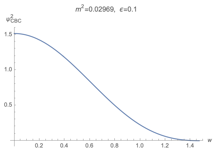
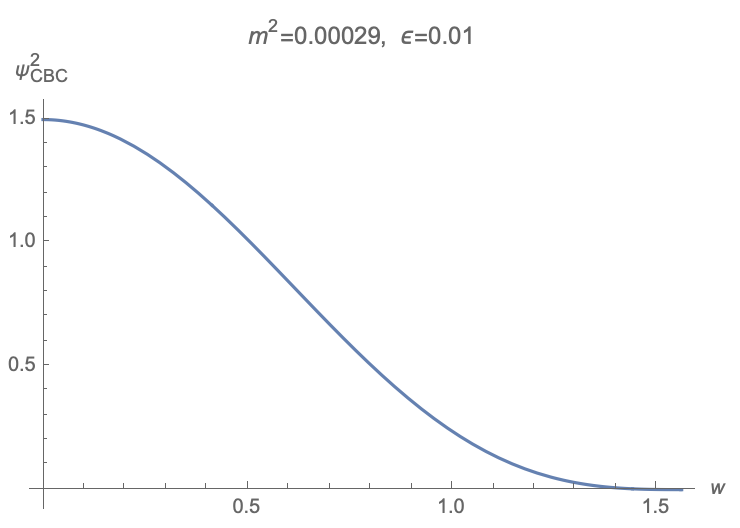
Figure 4: For CBC with zero brane tension, the first mode of massive gravity is localized on the brane in the sense that $\Psi^{2}_{\text{CBC}}(w)$ peaks on the brane $w=0$ only and decays when it goes far from the brane.

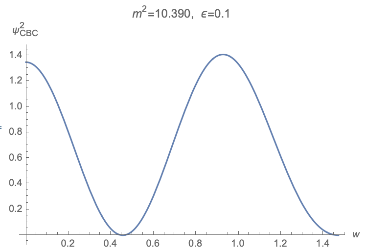
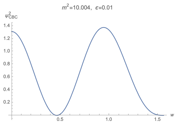
Figure 5: For CBC with zero brane tension, the second mode of massive gravity is not well-localized on the brane $w=0$.

In the above discussions, we have focused on the zero brane tension. To end this subsection, let us briefly discuss the case of non-zero brane tension. Following the above approach, let us draw the figures of wave functions. As shown in Fig. 6, for CBC with negative brane tension, the first mode of gravity is localized on the brane. While for CBC with positive brane tension, as shown in Fig. 7, the gravity is not well-localized on the brane. This agrees with the analysis of “volcanic potential” in section C.1.

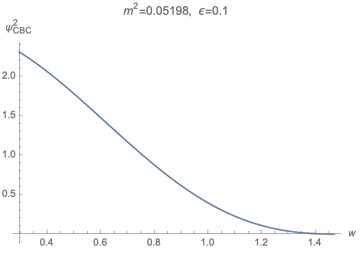
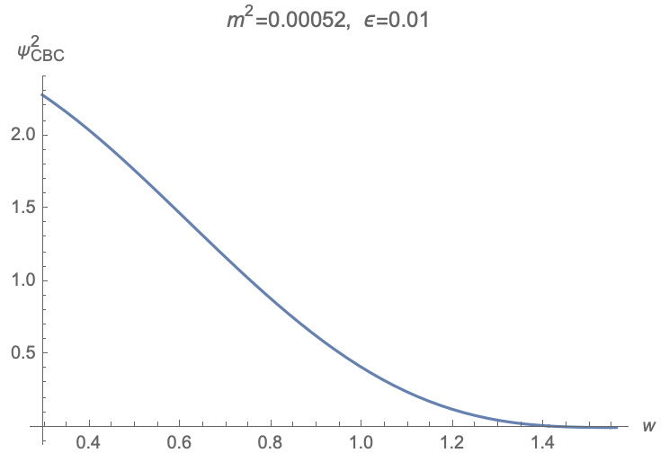
Figure 6: For CBC with negative brane tension $T=3\tanh\rho\approx-0.874$, the first mode of gravity is localized on the brane in the sense that $\Psi^{2}_{\text{CBC}}(w)$ peaks on the brane $w\approx 0.296$ only and decays when it goes far from the brane.

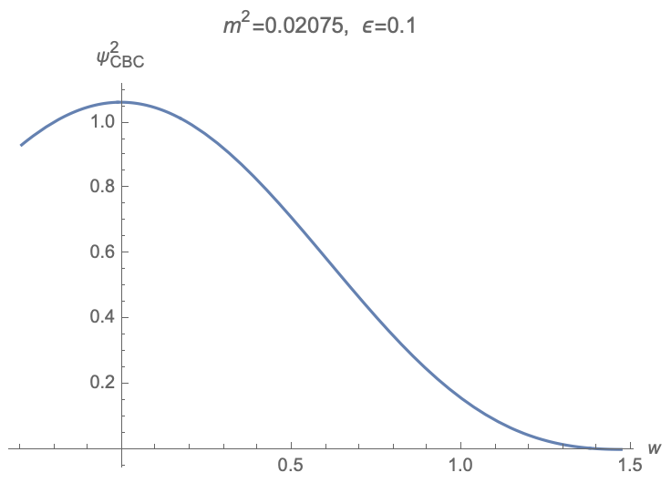
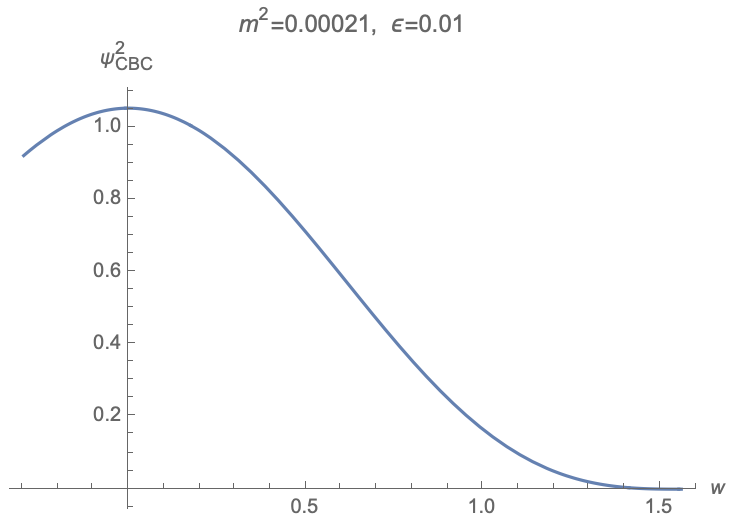
Figure 7: For CBC with positive brane tension $T=3\tanh\rho\approx 0.874$, the first mode of gravity is not well-localized on the brane at $w\approx-0.296$.

References

- [1] E. Witten, arXiv:1805.11559 [hep-th].
- [2] R. X. Miao, C. S. Chu and W. Z. Guo, Phys. Rev. D 96, no.4, 046005 (2017) [arXiv:1701.04275 [hep-th]].
- [3] C. S. Chu, R. X. Miao and W. Z. Guo, JHEP 04, 089 (2017) [arXiv:1701.07202 [hep-th]].
- [4] G. Penington, JHEP 09, 002 (2020) [arXiv:1905.08255 [hep-th]].
- [5] A. Almheiri, N. Engelhardt, D. Marolf and H. Maxfield, JHEP 12, 063 (2019) [arXiv:1905.08762 [hep-th]].
- [6] A. Almheiri, R. Mahajan, J. Maldacena and Y. Zhao, JHEP 03, 149 (2020) [arXiv:1908.10996 [hep-th]].
- [7] M. Rozali, J. Sully, M. Van Raamsdonk, C. Waddell and D. Wakeham, JHEP 05, 004 (2020) [arXiv:1910.12836 [hep-th]].
- [8] H. Z. Chen, Z. Fisher, J. Hernandez, R. C. Myers and S. M. Ruan, JHEP 03, 152 (2020) [arXiv:1911.03402 [hep-th]].
- [9] A. Almheiri, R. Mahajan and J. E. Santos, SciPost Phys. 9, no.1, 001 (2020) [arXiv:1911.09666 [hep-th]].
- [10] Y. Kusuki, Y. Suzuki, T. Takayanagi and K. Umemoto, [arXiv:1912.08423 [hep-th]].
- [11] V. Balasubramanian, A. Kar, O. Parrikar, G. Sárosi and T. Ugajin, [arXiv:2003.05448 [hep-th]].
- [12] J. Sully, M. Van Raamsdonk and D. Wakeham, [arXiv:2004.13088 [hep-th]].
- [13] H. Geng and A. Karch, JHEP 09 (2020), 121 [arXiv:2006.02438 [hep-th]].
- [14] H. Z. Chen, R. C. Myers, D. Neuenfeld, I. A. Reyes and J. Sandor, [arXiv:2006.04851 [hep-th]].
- [15] X. Dong, X. L. Qi, Z. Shangnan and Z. Yang, [arXiv:2007.02987 [hep-th]].
- [16] C. Arias, F. Diaz, R. Olea and P. Sundell, JHEP 04, 124 (2020) [arXiv:1906.05310 [hep-th]].
- [17] C. Arias, F. Diaz and P. Sundell, Class. Quant. Grav. 37, no.1, 015009 (2020) [arXiv:1901.04554 [hep-th]].
- [18] H. Geng, [arXiv:2005.00021 [hep-th]].
- [19] Y. Ling, Y. Liu and Z. Y. Xian, [arXiv:2010.00037 [hep-th]].
- [20] H. Geng, A. Karch, C. Perez-Pardavila, S. Raju, L. Randall, M. Riojas and S. Shashi, [arXiv:2012.04671 [hep-th]].
- [21] K. Kawabata, T. Nishioka, Y. Okuyama and K. Watanabe, JHEP 05, 062 (2021) [arXiv:2102.02425 [hep-th]].
- [22] A. Bhattacharya, A. Bhattacharyya, P. Nandy and A. K. Patra, JHEP 05, 135 (2021) [arXiv:2103.15852 [hep-th]].
- [23] K. Kawabata, T. Nishioka, Y. Okuyama and K. Watanabe, [arXiv:2105.08396 [hep-th]].
- [24] H. Geng, A. Karch, C. Perez-Pardavila, S. Raju, L. Randall, M. Riojas and S. Shashi, [arXiv:2107.03390 [hep-th]].
- [25] C. Krishnan, JHEP 01, 179 (2021) [arXiv:2007.06551 [hep-th]].
- [26] F. Deng, J. Chu and Y. Zhou, JHEP 03, 008 (2021) [arXiv:2012.07612 [hep-th]].
- [27] J. Chu, F. Deng and Y. Zhou, [arXiv:2105.09106 [hep-th]].
- [28] D. Neuenfeld, [arXiv:2104.02801 [hep-th]].
- [29] D. Neuenfeld, [arXiv:2105.01130 [hep-th]].
- [30] H. Z. Chen, R. C. Myers, D. Neuenfeld, I. A. Reyes and J. Sandor, JHEP 12, 025 (2020) [arXiv:2010.00018 [hep-th]].
- [31] K. Ghosh and C. Krishnan, JHEP 08, 119 (2021) [arXiv:2103.17253 [hep-th]].
- [32] H. Omiya and Z. Wei, [arXiv:2107.01219 [hep-th]].
- [33] J. M. Maldacena, Int. J. Theor. Phys. 38, 1113 (1999) [Adv. Theor. Math. Phys. 2, 231 (1998)] [hep-th/9711200].
- [34] S. S. Gubser, I. R. Klebanov and A. M. Polyakov, Phys. Lett. B 428, 105-114 (1998) [arXiv:hep-th/9802109 [hep-th]].
- [35] E. Witten, Adv. Theor. Math. Phys. 2, 253-291 (1998) [arXiv:hep-th/9802150 [hep-th]].
- [36] L. Randall and R. Sundrum, Phys. Rev. Lett. 83, 3370-3373 (1999) [arXiv:hep-ph/9905221 [hep-ph]].
- [37] L. Randall and R. Sundrum, Phys. Rev. Lett. 83, 4690-4693 (1999) [arXiv:hep-th/9906064 [hep-th]].
- [38] A. Karch and L. Randall, JHEP 05, 008 (2001) [arXiv:hep-th/0011156 [hep-th]].
- [39] T. Takayanagi, Phys. Rev. Lett. 107 (2011) 101602 [arXiv:1105.5165 [hep-th]].
- [40] M. Fujita, T. Takayanagi and E. Tonni, JHEP 11, 043 (2011) [arXiv:1108.5152 [hep-th]].
- [41] M. Nozaki, T. Takayanagi and T. Ugajin, JHEP 06, 066 (2012) [arXiv:1205.1573 [hep-th]].
- [42] R. X. Miao, JHEP 02, 025 (2019) [arXiv:1806.10777 [hep-th]].
- [43] J. L. Cardy, hep-th/0411189.
- [44] D. M. McAvity and H. Osborn, Nucl. Phys. B 406, 655 (1993) [hep-th/9302068].
- [45] I. Akal, Y. Kusuki, T. Takayanagi and Z. Wei, Phys. Rev. D 102, no.12, 126007 (2020) [arXiv:2007.06800 [hep-th]].
- [46] R. Bousso and E. Wildenhain, Phys. Rev. D 102, no.6, 066005 (2020) [arXiv:2006.16289 [hep-th]].
- [47] R. X. Miao, JHEP 01, 150 (2021) [arXiv:2009.06263 [hep-th]].
- [48] R. X. Miao, Phys. Rev. D 104, no.8, 8 (2021) [arXiv:2101.10031 [hep-th]].
- [49] R. X. Miao and C. S. Chu, JHEP 1803, 046 (2018) [arXiv:1706.09652 [hep-th]].
- [50] M. T. Anderson, Geom. Topol. 12, no.4, 2009-2045 (2008) [arXiv:math/0612647 [math.DG]].
- [51] M. T. Anderson, Selecta Math. 16 (2010) 343-375, [arXiv:0704.3373 [math.DG]].
- [52] M. T. Anderson, Phys. Rev. D 82, 084044 (2010) [arXiv:1008.4309 [gr-qc]].
- [53] J. W. York, Jr., Phys. Rev. Lett. 28, 1082-1085 (1972)
- [54] I. Papadimitriou and K. Skenderis, JHEP 08, 004 (2005) [arXiv:hep-th/0505190 [hep-th]].
- [55] D. Deutsch and P. Candelas, Phys. Rev. D 20, 3063 (1979).
- [56] K. Jensen and A. O’Bannon, Phys. Rev. Lett. 116, no. 9, 091601 (2016) [arXiv:1509.02160 [hep-th]].
- [57] C. P. Herzog, K. W. Huang and K. Jensen, JHEP 1601, 162 (2016) [arXiv:1510.00021 [hep-th]].
- [58] D. Fursaev, JHEP 1512, 112 (2015) [arXiv:1510.01427 [hep-th]].
- [59] S. N. Solodukhin, Phys. Lett. B 752, 131 (2016) [arXiv:1510.04566 [hep-th]].
- [60] R. X. Miao, JHEP 07, 098 (2019) [arXiv:1808.05783 [hep-th]].
- [61] C. S. Chu and R. X. Miao, Phys. Rev. Lett. 121, no.25, 251602 (2018) [arXiv:1803.03068 [hep-th]].
- [62] C. S. Chu and R. X. Miao, JHEP 07, 005 (2018) [arXiv:1804.01648 [hep-th]].
- [63] C. S. Chu and R. X. Miao, JHEP 07, 151 (2019) [arXiv:1812.10273 [hep-th]].
- [64] C. S. Chu, Fortsch. Phys. 67, no.8-9, 1910005 (2019) [arXiv:1903.02817 [hep-th]].
- [65] C. S. Chu and R. X. Miao, Phys. Rev. D 102, no.4, 046011 (2020) [arXiv:2004.05780 [hep-th]].
- [66] C. S. Chu and R. X. Miao, JHEP 08, 134 (2020) [arXiv:2005.12975 [hep-th]].
- [67] M. Billò, V . Goncalves, E. Lauria and M. Meineri, JHEP 1604, 091 (2016) [arXiv:1601.02883 [hep-th]].
- [68] C. Herzog, K. W. Huang and K. Jensen, Phys. Rev. Lett. 120, no. 2, 021601 (2018) [arXiv:1709.07431 [hep-th]].
- [69] C. P. Herzog and K. W. Huang, JHEP 1710, 189 (2017) [arXiv:1707.06224 [hep-th]].
- [70] M. Henningson and K. Skenderis, JHEP 9807 (1998) 023 [hep-th/9806087].
- [71] Magnus W , Oberhettinger F , Soni R, “Formulas and Theorems for the Special Functions of Mathematical Physics”, American Journal of Physics 35, 550 (1967).
- [72] A. Karch and Y. Sato, JHEP 07 (2018), 156 [arXiv:1805.10427 [hep-th]].
- [73] A. Bissi, T. Hansen and A. Söderberg, JHEP 01, 010 (2019) [arXiv:1808.08155 [hep-th]].
- [74] D. Mazáč, L. Rastelli and X. Zhou, JHEP 12, 004 (2019) [arXiv:1812.09314 [hep-th]].
- [75] W. Reeves, M. Rozali, P. Simidzija, J. Sully, C. Waddell and D. Wakeham, [arXiv:2108.10345 [hep-th]].
- [76] J. Kastikainen and S. Shashi, [arXiv:2109.00079 [hep-th]].
- [77] S. Rychkov, [arXiv:1601.05000 [hep-th]].
- [78] D. Simmons-Duffin, [arXiv:1602.07982 [hep-th]].
- [79] D. Poland, S. Rychkov and A. Vichi, Rev. Mod. Phys. 91, 015002 (2019) doi:10.1103/RevModPhys.91.015002 [arXiv:1805.04405 [hep-th]].