The Benefits of Being Categorical Distributional:
Uncertainty-aware Regularized Exploration in Reinforcement Learning

Abstract

The theoretical advantages of distributional reinforcement learning (RL) over classical RL remain elusive despite its remarkable empirical performance. Starting from Categorical Distributional RL (CDRL), we attribute the potential superiority of distributional RL to a derived distribution-matching regularization by applying a return density function decomposition technique. This unexplored regularization in the distributional RL context is aimed at capturing additional return distribution information regardless of only its expectation, contributing to an augmented reward signal in the policy optimization. Compared with the entropy regularization in MaxEnt RL that explicitly optimizes the policy to encourage the exploration, the resulting regularization in CDRL implicitly optimizes policies guided by the new reward signal to align with the uncertainty of target return distributions, leading to an uncertainty-aware exploration effect. Finally, extensive experiments substantiate the importance of this uncertainty-aware regularization in distributional RL on the empirical benefits over classical RL.

1 Introduction

The intrinsic characteristics of classical reinforcement learning (RL) algorithms, such as Q-learning (Sutton & Barto, 2018; Watkins & Dayan, 1992), are based on the expectation of discounted cumulative rewards that an agent observes while interacting with the environment. In stark contrast to the expectation-based RL, a new branch of algorithms called distributional RL estimates the full distribution of total returns and has demonstrated the state-of-the-art performance in a wide range of environments (Bellemare et al., 2017a; Dabney et al., 2018b, a; Yang et al., 2019; Zhou et al., 2020; Nguyen et al., 2020; Sun et al., 2022b). Meanwhile, distributional RL also inherits other benefits in risk-sensitive control (Dabney et al., 2018a; Lim & Malik, 2022; Cho et al., 2023), offline learning (Wu et al., 2023; Ma et al., 2021), policy exploration settings (Mavrin et al., 2019; Rowland et al., 2019), robustness (Sun et al., 2023; Sui et al., 2023) and optimization (Sun et al., 2022a; Rowland et al., 2023b; Kuang et al., 2023). Despite numerous algorithmic variants of distributional RL with remarkable empirical success, we still have a poor understanding of the effectiveness of distributional RL. The theoretical advantages of distributional RL over expectation-based RL are still less studied.

In this paper, we illuminate the behavior difference of distributional RL over expectation-based RL starting from CDRL (Bellemare et al., 2017a), the first successful distributional RL family. Firstly, we decompose the distributional RL objective function into an expectation-based term and a distribution-matching regularization via the return density function decomposition, a variant of the gross error model in robust statistics. Furthermore, the resulting regularization serves as an augmented reward in the actor-critic framework, encouraging the policies to explore states and actions whose current return distribution estimate lags far behind the target one determined by the environment. This leads to an uncertainty-aware exploration effect in contrast to the exploration for diverse actions in MaxEnt RL. Meanwhile, we propose a theoretically principled algorithm called Distribution-Entropy-Regularized Actor Critic accordingly, interpolating between expectation-based and distributional RL. Empirical results demonstrate the crucial role of the uncertainty-aware entropy regularization from CDRL in its empirical success over expectation-based RL on both Atari games and MuJoCo environments. We also reveal the mutual impacts of the uncertainty-aware entropy in distributional RL and the explicit vanilla entropy in MaxEnt RL, providing more potential research directions in the future. Our contributions are summarized as follows:

1) We propose a return density decomposition technique to decompose the objective function in CDRL, yielding an uncertainty-aware regularization that is helpful to interpret the benefits of CDRL over expectation-based RL.

2) We incorporate the uncertainty-aware regularization into the actor-critic framework, encouraging uncertainty-aware exploration compared with MaxEnt RL. We also propose a theoretically grounded actor-critic algorithm, interpolating between classical and distributional RL.

3) Empirically, we verify the impact of the uncertainty-aware regularization on the empirical advantage of distributional RL over classical RL and show the mutual impact of the two types of regularization.

2 Related Work

The theoretical properties of CDRL were first revealed in (Rowland et al., 2018), drawing fundamental connections between CDRL and Cramér distance. However, the empirical superiority of CDRL is not yet well understood. For the general distributional RL, previous works (Lyle et al., 2019) proved that in many realizations of tabular and linear approximation settings, distributional RL behaves the same as expectation-based RL under the coupling updates method, but it diverges in non-linear approximation. As an essential complementary result, our work focuses on practical distributional RL algorithms with non-linear approximation starting from CDRL, the first successful distributional RL class. Moreover, asymptotic convergence guarantees of popular distributional RL algorithms, such as QR-DQN (Dabney et al., 2018b), were proved in (Rowland et al., 2023a), but they may not explain the benefits of distributional RL approaches as they do not imply stronger finite-sample guarantees than classical RL. A recent work (Wu et al., 2023) explained the benefits of distributional RL from the perspective of the small-loss PAC bounds. However, their results are mainly on low-rank MDP instead of considering the general function approximation.

3 Preliminaries

In classical RL, an agent interacts with an environment via Markov Decision Process (MDP), a 5-tuple ($\mathcal{S},\mathcal{A},R,P,\gamma$), where $\mathcal{S}$ and $\mathcal{A}$ are the state and action spaces, $P$ is the environment state transition dynamics, $R$ is the reward function and $\gamma\in(0,1)$ is the discount factor.

Action-State Value Function vs Action-State Return Distribution. Given a policy $\pi$, the discounted sum of future rewards is a random variable $Z^{\pi}(s,a)=\sum_{t=0}^{\infty}\gamma^{t}R(s_{t},a_{t})$, where $s_{0}=s$, $a_{0}=a$, $s_{t+1}\sim P(\cdot|s_{t},a_{t})$, and $a_{t}\sim\pi(\cdot|s_{t})$. In the control setting, expectation-based RL focuses on the action-value function $Q^{\pi}(s,a)$, the expectation of $Z^{\pi}(s,a)$, i.e., $Q^{\pi}(s,a)=\mathbb{E}\left[Z^{\pi}(s,a)\right]$. Distributional RL, on the other hand, focuses on the action-state return distribution, the full distribution of $Z^{\pi}(s,a)$. We call its density as action-state return density function.

Bellman Operators vs Distributional Bellman Operators. In the policy evaluation of classical RL, the value function is updated via the Bellman operator $\mathcal{T}^{\pi}Q(s,a)=\mathbb{E}[R(s,a)]+\gamma\mathbb{E}_{s^{\prime}\sim p,a^{\prime}\sim\pi}\left[Q\left(s^{\prime},a^{\prime}\right)\right]$. We also define Bellman Optimality Operator $\mathcal{T}^{\text{opt}}Q(s,a)=\mathbb{E}[R(s,a)]+\gamma\max_{a^{\prime}}\mathbb{E}_{s^{\prime}\sim p}\left[Q\left(s^{\prime},a^{\prime}\right)\right]$. In distributional RL, the action-state return distribution of $Z^{\pi}(s,a)$ is updated via the distributional Bellman operator $\mathfrak{T}^{\pi}$, i.e., $\mathfrak{T}^{\pi}Z(s,a)\stackrel{{\scriptstyle D}}{{=}}R(s,a)+\gamma Z\left(s^{\prime},a^{\prime}\right)$, where $s^{\prime}\sim P(\cdot|s,a)$, $a^{\prime}\sim\pi\left(\cdot|s^{\prime}\right)$ and $\stackrel{{\scriptstyle D}}{{=}}$ implies random variables of both sides are equal in distribution. We use this random-variable definition of $\mathfrak{T}^{\pi}$, which is appealing and easily understood due to its concise form (Rowland et al., 2018; Bellemare et al., 2022).

Categorical Distributional RL (CDRL). CDRL (Bellemare et al., 2017a) can be viewed as the first successful distributional RL algorithm family that approximates the return distribution $\eta$ by a discrete categorical distribution $\hat{\eta}=\sum_{i=1}^{N}p_{i}\delta_{z_{i}}$, where $\{z_{i}\}_{i=1}^{N}$ is a set of fixed supports and $\{p_{i}\}_{i=1}^{N}$ are learnable probabilities. The usage of a heuristic projection operator $\Pi_{\mathcal{C}}$ (see Appendix A for more details) as well as the KL divergence allows the theoretical convergence of categorical distribution RL under Cramér distance or Wasserstein distance (Rowland et al., 2018).

4 Uncertainty-aware Regularized Exploration in Value-based Distributional RL

4.1 Distributional RL: Neural FZI

Expectation-based RL: Neural Fitted Q-Iteration (Neural FQI). Neural FQI (Fan et al., 2020; Riedmiller, 2005) offers a statistical explanation of DQN (Mnih et al., 2015), capturing its key features, including experience replay and the target network $Q_{\theta^{*}}$. In Neural FQI, we update a parameterized $Q_{\theta}$ in each iteration $k$ in a regression problem:

$$Q_{\theta}^{k+1}=\underset{Q_{\theta}}{\operatorname{argmin}}\frac{1}{n}\sum_{i=1}^{n}\left[y_{i}^{k}-Q_{\theta}\left(s_{i},a_{i}\right)\right]^{2},$$ (1)

where the target $y_{i}^{k}=r(s_{i},a_{i})+\gamma\max_{a\in\mathcal{A}}Q^{k}_{\theta^{*}}\left(s_{i}^{\prime},a\right)$ is fixed within every $T_{\text{target}}$ steps to update target network $Q_{\theta^{*}}$ by letting $Q_{\theta^{*}}^{k+1}=Q_{\theta}^{k+1}$. The experience buffer induces independent samples $\left\{\left(s_{i},a_{i},r_{i},s_{i}^{\prime}\right)\right\}_{i\in[n]}$. If $\{Q_{\theta}:\theta\in\Theta\}$ is sufficiently large such that it contains $\mathcal{T}^{\text{opt}}Q_{\theta^{*}}^{k}$, Eq. 1 has solution $Q_{\theta}^{k+1}=\mathcal{T}^{\text{opt}}Q_{\theta^{*}}^{k}$, which is exactly the updating rule under Bellman optimality operator (Fan et al., 2020). From the statistics viewpoint, the optimization problem in Eq. 1 in each iteration is a standard supervised and neural network parameterized regression regarding $Q_{\theta}$.

Distributional RL: Neural Fitted Z-Iteration (Neural FZI). We interpret distributional RL as Neural FZI as it is by far closest to the practical algorithms, although our analysis is not intended to involve properties of neural networks. Analogous to Neural FQI, we can simplify value-based distributional RL algorithms parameterized by $Z_{\theta}$ into Neural FZI as

$$Z_{\theta}^{k+1}=\underset{Z_{\theta}}{\operatorname{argmin}}\frac{1}{n}\sum_{i=1}^{n}d_{p}(Y_{i}^{k},Z_{\theta}\left(s_{i},a_{i}\right)),$$ (2)

where the target $Y_{i}^{k}=R(s_{i},a_{i})+\gamma Z^{k}_{\theta^{*}}\left(s_{i}^{\prime},\pi_{Z}(s_{i}^{\prime})\right)$ with the policy $\pi_{Z}$ following the greedy rule $\pi_{Z}(s^{\prime}_{i})=\operatorname{argmax}_{a^{\prime}}\mathbb{E}\left[Z_{\theta^{*}}^{k}(s_{i}^{\prime},a^{\prime})\right]$ is fixed within every $T_{\text{target}}$ steps to update target network $Z_{\theta^{*}}$. $d_{p}$ is a divergence between two distributions, and here, the lower cases random variables $s_{i}^{\prime}$ and $\pi_{Z}(s_{i}^{\prime})$ are given for convenience.

4.2 Distributional RL: Entropy-regularized Neural FQI

Return Density Function Decomposition. To separate the impact of additional distribution information from the expectation of $Z^{\pi}$, we use a variant of gross error model from robust statistics (Huber, 2004), which was also similarly used to analyze Label Smoothing (Müller et al., 2019) and Knowledge Distillation (Hinton et al., 2015). Akin to the categorical representation in CDRL (Dabney et al., 2018b), we utilize a histogram function estimator $\widehat{p}^{s,a}(x)$ with $N$ bins to approximate an arbitrary continuous true action-value density $p^{s,a}(x)$ given a state $s$ and action $a$. We leverage the continuous histogram estimator rather than the discrete categorical parameterization for richer analysis. Given a fixed set of supports $l_{0}\leq l_{1}\leq...\leq l_{N}$ with the equal bin size as $\Delta$, $\Delta_{i}=[l_{i-1},l_{i})$, $i=1,...,N-1$ with $\Delta_{N}=[l_{N-1},l_{N}]$, the histogram density estimator is $\widehat{p}^{s,a}(x)=\sum_{i=1}^{N}p_{i}\mathds{1}(x\in\Delta_{i})/\Delta$ with $p_{i}$ as the coefficient in the $i$-th bin. Denote $\Delta_{E}$ as the interval that $\mathbb{E}\left[Z^{\pi}(s,a)\right]$ falls into, i.e., $\mathbb{E}\left[Z^{\pi}(s,a)\right]\in\Delta_{E}$. Putting all together, we have an action-state return density function decomposition over the histogram density estimator $\widehat{p}^{s,a}(x)$:

$$\widehat{p}^{s,a}(x) =(1-\epsilon)\mathds{1}(x\in\Delta_{E})/\Delta+\epsilon\widehat{\mu}^{s,a}(x)$$ (3)

where $\widehat{p}^{s,a}$ is decomposed into a single-bin histogram $\mathds{1}(x\in\Delta_{E})/\Delta$ with all mass on $\Delta_{E}$ and an induced histogram density function $\widehat{\mu}^{s,a}$ evaluated by $\widehat{\mu}^{s,a}(x)=\sum_{i=1}^{N}p^{\mu}_{i}\mathds{1}(x\in\Delta_{i})/\Delta$ with $p_{i}^{\mu}$ as the coefficient of the $i$-th bin. $\epsilon$ is a pre-specified hyper-parameter before the decomposition, controlling the proportion between $\mathds{1}(x\in\Delta_{E})/\Delta$ and $\widehat{\mu}^{s,a}(x)$. More specifically, the induced histogram $\widehat{\mu}^{s,a}$ in the second term is the difference between the considered histogram $\widehat{p}^{s,a}$ and a single-bin histogram, aiming at characterizing the impact of action-state return distribution despite its expectation $\mathbb{E}\left[Z^{\pi}(s,a)\right]$ on the performance of distributional RL. Optimizing the first term in Eq. 3 of Neural FZI is linked with Neural FQI for expectation-based RL, which we will show later. We also show that $\widehat{\mu}^{s,a}$ is a valid density function under certain $\epsilon$ in Proposition 4.1.

Proposition 4.1.

(Decomposition Validity) Denote $\widehat{p}^{s,a}(x\in\Delta_{E})=p_{E}/\Delta$ with $p_{E}$ as the coefficient on the bin $\Delta_{E}$. $\widehat{\mu}^{s,a}(x)=\sum_{i=1}^{N}p^{\mu}_{i}\mathds{1}(x\in\Delta_{i})/\Delta$ is a valid density function if and only if $\epsilon\geq 1-p_{E}$.

The proof is in Appendix B. Proposition 4.1 indicates that the return density function decomposition in Eq. 3 is valid when the pre-specified hyper-parameter $\epsilon$ satisfies $\epsilon\geq 1-p_{E}$, implying that $\epsilon\rightarrow 0$ is not attainable for a correct decomposition. Under this return density decomposition condition, our analysis maintains the standard categorical distribution framework in distributional RL.

Why Histogram Density Estimator? While the histogram function is a continuous estimator in contrast to the discrete nature of the categorical parameterization used in CDRL, we show that the histogram density estimator is equivalent to the categorical parameterization in Appendix C. Previous result (Rowland et al., 2018) derived a discrete categorical parameterization error bound to characterize the convergence between the true return distribution and the limiting one. As a complementary result, we provide a uniform convergence rate for the histogram density estimator in the context of distributional RL. Precisely, the sample-based histogram estimator can approximate any arbitrary continuous limiting density function under a mild condition. Please refer to Appendix D for more details.

Distributional RL: Entropy-regularized Neural FQI. We apply the decomposition on the target action-value histogram density function and choose KL divergence as $d_{p}$ in Neural FZI. Let $\mathcal{H}(U,V)$ be the cross-entropy between two probability measures $U$ and $V$, i.e., $\mathcal{H}(U,V)=-\int_{x\in\mathcal{X}}U(x)\log V(x)\mathrm{~{}d}x$. The target histogram density function $\widehat{p}^{s,a}$ is decomposed as $\widehat{p}^{s,a}(x)=(1-\epsilon)\mathds{1}(x\in\Delta_{E})/\Delta+\epsilon\widehat{\mu}^{s,a}(x)$. We can derive the following entropy-regularized form for distributional RL in Proposition 4.2 with the proof in Appendix F.

Proposition 4.2.

(Decomposed Neural FZI) Denote $q_{\theta}^{s,a}(x)$ as the histogram estimator of $Z^{k}_{\theta}(s,a)$ in Neural FZI. Based on Eq. 3 and KL divergence as $d_{p}$, Neural FZI in Eq. 2 is simplified as

$${Z}_{\theta}^{k+1}=\underset{q_{\theta}}{\operatorname{argmin}}\frac{1}{n}\sum_{i=1}^{n}[\underset{(a)}{\underbrace{-\log q^{s_{i},a_{i}}_{\theta}(\Delta^{i}_{E})}}$$ (4)

$$+\alpha\mathcal{H}(\widehat{\mu}^{s_{i}^{\prime},\pi_{Z}(s^{\prime}_{i})},q^{s_{i},a_{i}}_{\theta})],$$

where $\Delta_{E}^{i}$ represents the interval that the expectation of the target random variable $R(s_{i},a_{i})+\gamma Z^{k}_{\theta^{*}}\left(s_{i}^{\prime},\pi_{Z}(s_{i}^{\prime})\right)$ falls into, i.e., $\mathbb{E}\left[R(s_{i},a_{i})+\gamma Z^{k}_{\theta^{*}}\left(s_{i}^{\prime},\pi_{Z}(s_{i}^{\prime})\right)\right]\in\Delta_{E}^{i}$. $\alpha=\varepsilon/(1-\varepsilon)>0$ and $\widehat{\mu}^{s_{i}^{\prime},\pi_{Z}(s^{\prime}_{i})}$ is the induced histogram density function by decomposing the histogram density estimator of $R(s_{i},a_{i})+\gamma Z^{k}_{\theta^{*}}\left(s_{i}^{\prime},\pi_{Z}(s_{i}^{\prime})\right)$ via Eq. 3. In Proposition 4.3, we further show that minimizing the term (a) in Eq. 4 is equivalent to minimizing Neural FQI, and therefore, the regularization term $\alpha\mathcal{H}(\widehat{\mu}^{s_{i}^{\prime},\pi_{Z}(s^{\prime}_{i})},q^{s_{i},a_{i}}_{\theta})$ can suffice to interpret the benefits of CDRL over classical RL. For the uniformity of notation, we still use $s,a$ in the following analysis instead of $s_{i},a_{i}$.

Proposition 4.3.

(Equivalence between the term (a) in Decomposed Neural FZI and Neural FQI) In Eq. 4 of Neural FZI, assume the function class $\{Z_{\theta}:\theta\in\Theta\}$ is sufficiently large such that it contains the target $\{Y_{i}^{k}\}_{i=1}^{n}$ for all $k$, when $\Delta\rightarrow 0$, minimizing the term (a) in Eq. 4 implies

$$P(Z^{k+1}_{\theta}(s,a)=\mathcal{T}^{\text{opt}}Q^{k}_{\theta^{*}}(s,a))=1,$$ (5)

where $\mathcal{T}^{\text{opt}}Q^{k}_{\theta^{*}}(s,a)$ is the scalar-valued target in the k-th phase of Neural FQI.

The proof is given in Appendix G. Proposition 4.3 demonstrates that as $\Delta\rightarrow 0$, the random variable $Z^{k+1}_{\theta}(s,a)$ with the limiting distribution in Neural FZI (distributional RL) will degrade to a constant $\mathcal{T}^{\text{opt}}Q^{k}_{\theta^{*}}(s,a)$, the minimizer (scalar-valued target) in Neural FQI (classical RL). That being said, minimizing the term (a) in Neural FZI is equivalent to minimizing Neural FQI. See Appendix G for more results about the convergence rate $o(\Delta)$ in distribution. With the underlying link between optimizing the term (a) of Neural FZI with Neural FQI established in Proposition 4.3, it allows us to leverage the regularization term $\alpha\mathcal{H}(\widehat{\mu}^{s_{i}^{\prime},\pi_{Z}(s^{\prime}_{i})},q^{s_{i},a_{i}}_{\theta})$ to interpret the benefits of CDRL over classical RL. The assumption that $\{Z_{\theta}:\theta\in\Theta\}$ is sufficiently large such that it contains $\{Y_{i}^{k}\}_{i=1}^{n}$ indicates good in-distribution generalization performance in each phase of Neural FZI, which is commonly used in distributional RL context to derive tractable theoretical results, such as (Wu et al., 2023). Meanwhile, this connection with classic RL is also consistent with the mean-preserving property in classical RL (Rowland et al., 2018). Next, we are ready to elaborate on the impact of this regularization for Neural FZI (distributional RL).

4.3 Uncertainty-aware Regularized Exploration

Based on the equivalence between the term (a) of decomposed Neural FZI and FQI, the behavior difference of distributional RL compared with expectation-based RL can be attributed to the second regularization term $\mathcal{H}(\widehat{\mu}^{s_{i}^{\prime},\pi_{Z}(s^{\prime}_{i})},q^{s_{i},a_{i}}_{\theta})$. Minimizing Neural FZI pushes $q_{\theta}^{s,a}$ for the current return density estimator to catch up with the target return density function of $\widehat{\mu}^{s_{i}^{\prime},\pi_{Z}(s^{\prime}_{i})}$, which additionally incorporates the uncertainty of return distribution in the whole learning process instead of only encoding its expectation. Since it is a prevalent notion that distributional RL can significantly reduce intrinsic uncertainty of the environment (Mavrin et al., 2019; Dabney et al., 2018a), the derived distribution-matching regularization term helps the learning algorithms to capture more uncertainty of the environment by modeling the whole return distribution instead of only its expectation, leading to an uncertainty-aware regularized exploration effect.

Approximation of $\widehat{\mu}^{s^{\prime},\pi_{Z}(s^{\prime})}$. As in practical distributional RL algorithms, we typically use temporal-difference (TD) learning to attain the target probability density estimate $\widehat{\mu}^{s^{\prime},\pi_{Z}(s^{\prime})}$ based on Eq. 3 as long as $\mathbb{E}\left[Z(s,a)\right]$ exists and $\epsilon\geq 1-p_{E}$ in Proposition 4.1. The approximation error of $\widehat{\mu}^{s^{\prime},\pi_{Z}(s^{\prime})}$ is fundamentally determined by the TD learning nature. We also discuss the usage of KL divergence in Appendix E.

5 Uncertainty-aware Regularized Exploration in Actor Critic Framework

In this section, we further investigate the uncertainty-aware regularization and its exploration effect in the actor-critic framework by comparing it with MaxEnt RL.

5.1 Connection with MaxEnt RL

Explicit Entropy Regularization in MaxEnt RL. MaxEnt RL (Williams & Peng, 1991), including Soft Q-Learning (Haarnoja et al., 2017), explicitly encourages the exploration by optimizing for policies that aim to reach states where they will have high entropy in the future:

$$J(\pi)=\sum_{t=0}^{T}\mathbb{E}_{\left(s_{t},{a}_{t}\right)\sim\rho_{\pi}}\left[r\left({s}_{t},{a}_{t}\right)+\beta\mathcal{H}(\pi(\cdot|s_{t}))\right],$$ (6)

where $\mathcal{H}\left(\pi_{\theta}\left(\cdot|s_{t}\right)\right)=-\sum_{a}\pi_{\theta}\left(a|s_{t}\right)\log\pi_{\theta}\left(a|s_{t}\right)$ and $\rho_{\pi}$ is the generated distribution following $\pi$. The temperature parameter $\beta$ determines the relative importance of the entropy term against the cumulative rewards and thus controls the action diversity of the optimal policy learned via Eq. 6. This maximum entropy regularization has various conceptual and practical advantages. Firstly, the learned policy is encouraged to visit states with high entropy in the future, thus promoting the exploration of diverse states (Han & Sung, 2021). It also considerably improves the learning speed (Mei et al., 2020) and therefore is widely used in state-of-the-art algorithms, e.g., Soft Actor-Critic (SAC) (Haarnoja et al., 2018). Similar empirical benefits of both distributional RL and MaxEnt RL motivate us to probe their underlying connection.

Implicit Entropy Regularization in Distributional RL. To make a direct comparison with MaxEnt RL, we need to specifically analyze the impact of the regularization term in Eq. 4, and therefore, we incorporate the distribution-matching regularization of distributional RL into the Actor Critic (AC) framework akin to MaxEnt RL. This allows us to consider a new soft Q-value, i.e., the expectation of $Z^{\pi}(s,a)$. The new Q function can be computed iteratively by applying a modified Bellman operator denoted as $\mathcal{T}^{\pi}_{d}$, which we call Distribution-Entropy-Regularized Bellman Operator defined as

$$\mathcal{T}_{d}^{\pi}Q\left({s}_{t},{a}_{t}\right)\triangleq r\left({s}_{t},{a}_{t}\right)+\gamma\mathbb{E}_{{s}_{t+1}\sim P(\cdot|s_{t},a_{t})}\left[V\left({s}_{t+1}|s_{t},a_{t}\right)\right],$$ (7)

where a new soft value function $V\left({s}_{t+1}|s_{t},a_{t}\right)$ conditioned on $s_{t},a_{t}$ is defined by

$$V\left({s}_{t+1}|s_{t},a_{t}\right)=\mathbb{E}_{{a}_{t+1}\sim\pi}\left[Q\left({s}_{t+1},{a}_{t+1}\right)\right]$$ (8)

$$+f(\mathcal{H}\left(\mu^{s_{t},a_{t}},q_{\theta}^{s_{t},a_{t}}\right)),$$

where $f$ is a continuous increasing function over the cross-entropy $\mathcal{H}$ and $\mu^{s_{t},a_{t}}$ is the induced true target return histogram density function via the decomposition in Eq. 3 regardless of its expectation, which can be approximated via bootstrap estimate $\widehat{\mu}^{s_{t+1},\pi_{Z}\left(s_{t+1}\right)}$ similar in Eq. 4. In this specific tabular setting regarding $s_{t},a_{t}$, we particularly use $q_{\theta}^{s_{t},a_{t}}$ to approximate the true density function of $Z(s_{t},a_{t})$. The $f$ transformation over the cross-entropy $\mathcal{H}$ between $\mu^{s_{t},a_{t}}$ and $q_{\theta}^{s_{t},a_{t}}(x)$ serves as the uncertainty-aware entropy regularization that we implicitly derive from value-based distributional RL in Section 4.2. By optimizing the value-based critic component in Actor-Critic, i.e., $q_{\theta}$, this regularization reduces the mismatch between the target return distribution and current estimate, which is consistent with the regularization effect analyzed in Section 4.3. As illustrated in Figure 1, $q_{\theta}^{s,a}$ is optimized to catch up with the uncertainty of the target return distribution of $\mu^{s,a}$, thus increasing the knowledge of learning algorithms about the environment uncertainty for more informative decisions. Next, we elaborate on its additional impact on policy learning in the actor-critic framework in contrast to MaxEnt RL.

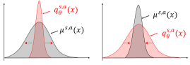
Figure 1: Uncertainty-aware distribution-matching regularization in CDRL to capture the intrinsic uncertainty of the environment. $q_{\theta}^{s,a}$ is forced to disperse (left) or concentrate (right) to align with the target return distribution.

Reward Augmentation for Policy Learning. As opposed to the vanilla entropy regularization in MaxEnt RL that explicitly encourages the policy to explore, our derived distribution-matching regularization in distributional RL plays a role of reward augmentation for policy learning. The augmented reward incorporates additional return distribution knowledge in the learning process compared with expectation-based RL. As we will show later, the augmented reward encourages policies to reach states $s_{t}$ with the following actions $a_{t}\sim\pi(\cdot|s_{t})$, whose current action-state return distribution $q_{\theta}^{s_{t},a_{t}}$ lag far behind the target ones, measured by the magnitude of cross entropy.

For a comprehensive analysis and a detailed comparison with MaxEnt RL, we now concentrate on the properties of our distribution-matching regularization in the Actor Critic (AC) framework. In Lemma 5.1, we first show that our Distribution-Entropy-Regularized Bellman operator $\mathcal{T}_{d}^{\pi}$ still inherits the convergence property in the policy evaluation phase with a cumulative augmented reward function as the new objective function $J^{\prime}(\pi)$.

Lemma 5.1.

(Distribution-Entropy-Regularized Policy Evaluation) Consider the distribution-entropy-regularized Bellman operator $\mathcal{T}_{d}^{\pi}$ in Eq. 7 and assume $\mathcal{H}(\mu^{s_{t},a_{t}},q_{\theta}^{s_{t},a_{t}})$ is bounded for all $(s_{t},a_{t})\in\mathcal{S}\times\mathcal{A}$. Define $Q^{k+1}=\mathcal{T}_{d}^{\pi}Q^{k}$, then $Q^{k+1}$ will converge to a corrected Q-value of $\pi$ as $k\rightarrow\infty$ with the new objective function $J^{\prime}(\pi)$ defined as

$$J^{\prime}(\pi)=\sum_{t=0}^{T}\mathbb{E}_{\left({s}_{t},{a}_{t}\right)\sim\rho_{\pi}}\left[r\left({s}_{t},{a}_{t}\right)+\gamma f(\mathcal{H}\left(\mu^{s_{t},a_{t}},q_{\theta}^{s_{t},a_{t}}\right))\right].$$ (9)

In the policy improvement phase, we keep the vanilla updating rules $\pi_{\text{new }}=\arg\max_{\pi^{\prime}\in\Pi}\mathbb{E}_{a_{t}\sim\pi^{\prime}}\left[Q^{\pi_{\text{old}}}(s_{t},a_{t})\right].$ Next, we can immediately derive a new policy iteration algorithm, called Distribution-Entropy-Regularized Policy Iteration (DERPI) that alternates between the policy evaluation in Eq. 7 and the policy improvement. It will provably converge to the policy regularized by the distribution-matching term as shown in Theorem 5.2.

Theorem 5.2.

(Distribution-Entropy-Regularized Policy Iteration) Repeatedly applying distribution-entropy-regularized policy evaluation in Eq. 7 and the policy improvement, the policy converges to an optimal policy $\pi^{*}$ such that $Q^{\pi^{*}}\left(s_{t},a_{t}\right)\geq Q^{\pi}\left(s_{t},a_{t}\right)$ for all $\pi\in\Pi$.

Please refer to Appendix H for the proof of Lemma 5.1 and Theorem 5.2. Theorem 5.2 demonstrates that if we incorporate the distribution-matching regularization into the policy gradient framework in Eq. 9, we can design a variant of “soft policy iteration” (Haarnoja et al., 2018) that can guarantee the convergence to an optimal policy, where the optimal policy is defined based on the optimal Q function (see the proof for more details). Putting all the analyses above together, we comprehensively compare the regularization and exploration effect between MaxEnt RL and distributional RL (CDRL).

Uncertainty-aware Regularized Exploration in CDRL Compared with MaxEnt RL. For the objective function $J(\pi)$ in Eq. 6 of MaxEnt RL, the state-wise entropy $\mathcal{H}(\pi(\cdot|s_{t}))$ is maximized explicitly w.r.t. $\pi$ for policies with a higher entropy in terms of diverse actions to encourage an explicit exploration. For the objective function $J^{\prime}(\pi)$ in Eq. 9 of distributional RL, the policy $\pi$ is implicitly optimized through the action selection $a_{t}\sim\pi(\cdot|s_{t})$ guided by an augmented reward signal from the distribution-matching regularization $f(\mathcal{H}\left(\mu^{s_{t},a_{t}},q_{\theta}^{s_{t},a_{t}}\right))$. Concretely, the learned policy is encouraged to visit state $s_{t}$ along with the policy-determined action via $a_{t}\sim\pi(\cdot|s_{t})$, whose current action-state return distributions $q_{\theta}^{s_{t},a_{t}}$ lag far behind the target return distributions, with a large magnitude of the cross entropy between two distributions. This results in an uncertainty-aware exploration against the environment driven by uncertainty difference (distribution mismatch) between the current return distribution estimate and the target one, which is the TD estimate of the environment uncertainty as analyzed in Eq. 4.

Interplay of Uncertainty-aware Regularization in Distributional Actor-Critic. Putting the critic and actor learning together in distributional RL, we reveal their interplay impact of the uncertainty-aware regularized exploration as opposed to expectation-based RL: 1) the actor (policy) learning seeks states and actions whose current return distribution estimate lag far behind the true one from the environment (approximated by the TD target distribution of $\mu^{s,a}$), 2) on the other hand, the critic learning reduces the return distribution mismatch on the explored states and actions between the current return distribution estimate and the true one determined by the environment, interpreting the benefits of CDRL over expectation-based RL.

5.2 DERAC Algorithm: Interpolating AC and Distributional AC

For a practical algorithm, we extend DERPI to the function approximation setting by parameterizing the return distribution $q_{\theta}(s_{t},a_{t})$ and the policy $\pi_{\phi}(a_{t}|s_{t})$ by neural networks. It turns out that the resulting Distribution-Entropy-Regularized Actor-Critic (DERAC) algorithm can interpolate expectation-based AC and distributional AC.

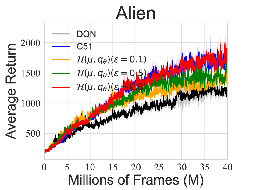
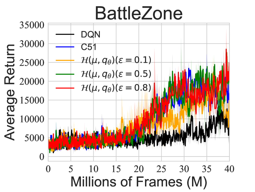
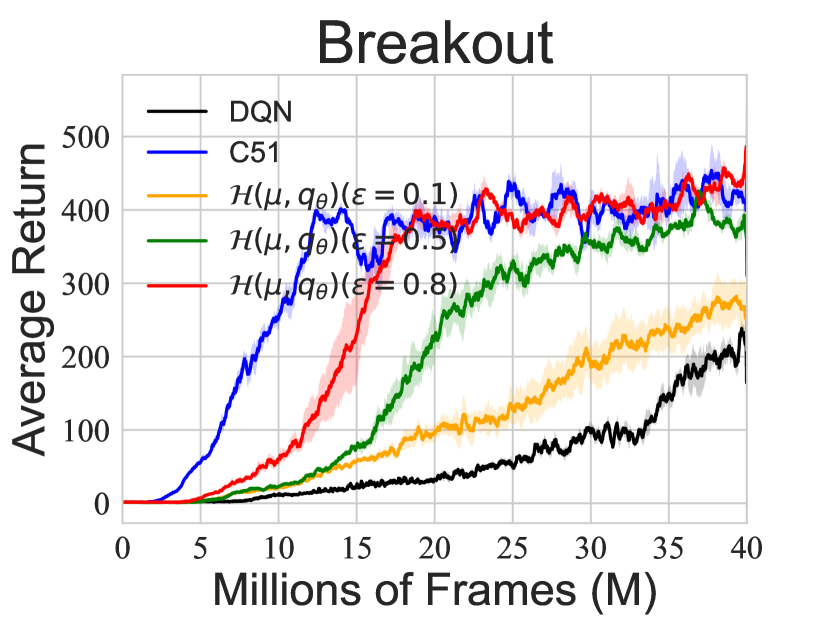
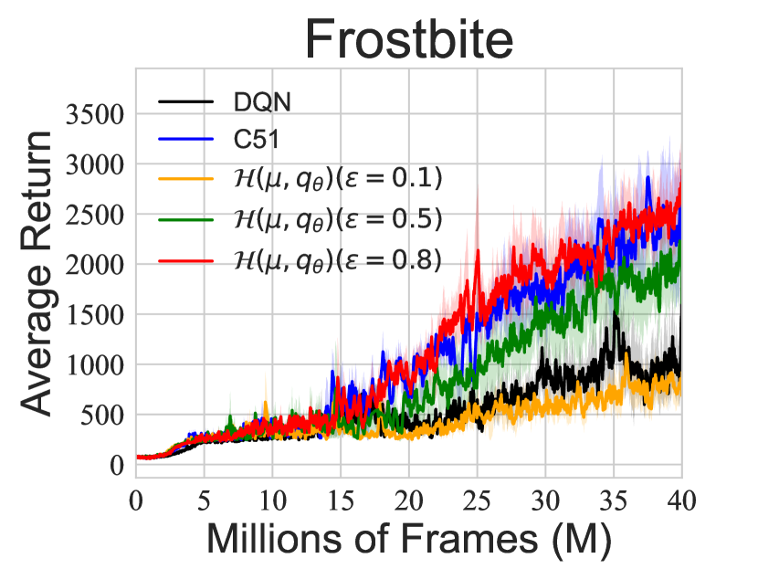
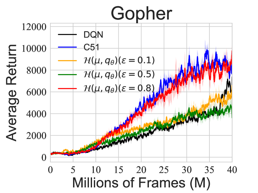
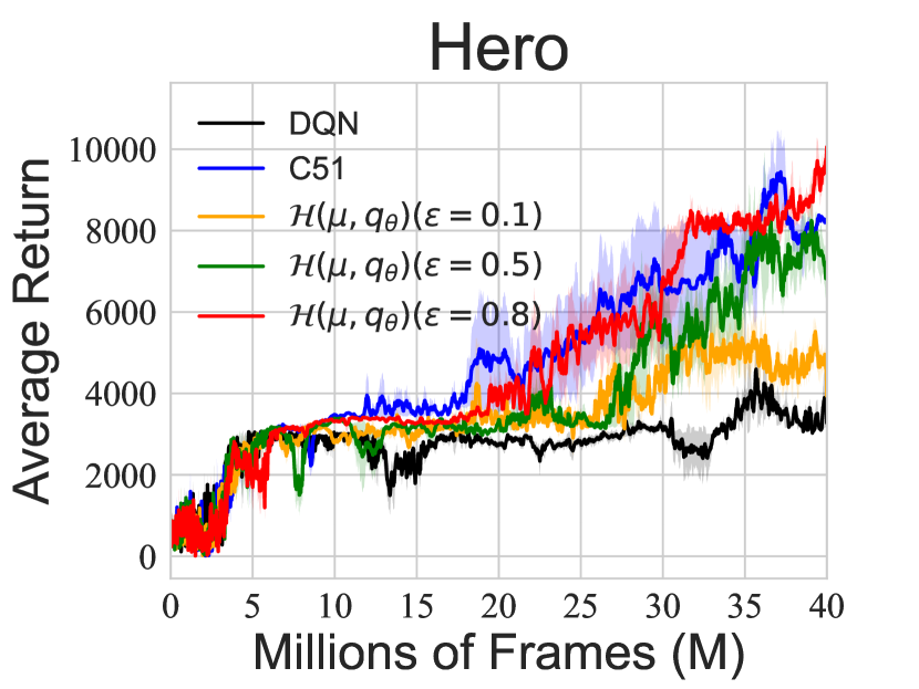
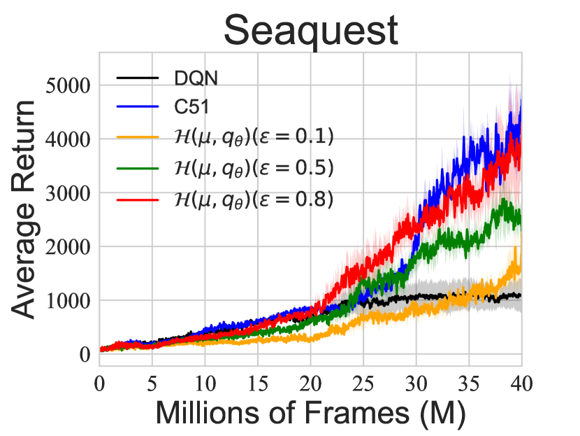
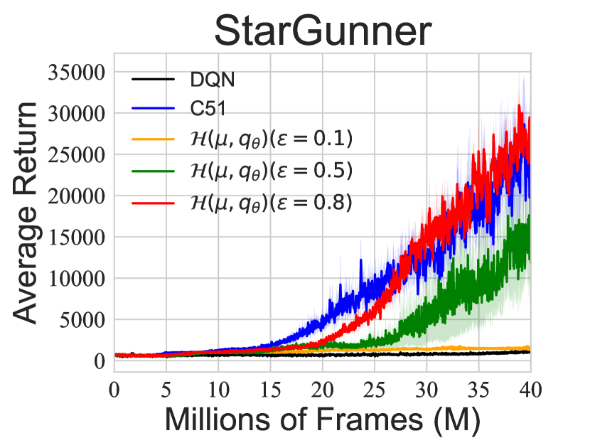
Figure 2: Learning curves of value-based CDRL, i.e., C51 algorithm, with return distribution decomposition $\mathcal{H}(\mu,q_{\theta})$ under different $\varepsilon$ on eight typical Atari games averaged over 3 seeds.

Optimize the critic by $q_{\theta}$. The new value function $\hat{J}_{q}(\theta)$ is originally trained to minimize the squared residual error of Eq. 7. We show that $\hat{J}_{q}(\theta)$ can be simplified as:

$$\hat{J}_{q}(\theta) \propto(1-\lambda)\mathbb{E}_{s,a}\left[\left(\mathcal{T}^{\pi}\mathbb{E}\left[q_{\theta^{*}}(s,a)\right]-\mathbb{E}\left[q_{\theta}(s,a)\right]\right)^{2}\right]$$ (10)

$$+\lambda\mathbb{E}_{s,a}\left[\mathcal{H}(\mu^{s,a},q_{\theta}^{s,a})\right],$$

where we use a particular increasing function $f(\mathcal{H})=(\tau\mathcal{H})^{\frac{1}{2}}/\gamma$ and $\lambda=\frac{\tau}{1+\tau}\in[0,1],\tau\geq 0$ is the hyperparameter that controls the uncertainty-aware regularization effect. The proof is given in Appendix I. Interestingly, when we leverage the whole target density function $\widehat{p}^{s,a}$ to approximate the true return distribution of $\mu^{s,a}$, the objective function in Eq. 10 can be viewed as an exact interpolation of loss functions between expectation-based AC (the first term) and categorical distributional AC loss (the second term) (Ma et al., 2020). In our implementation, for the target $\mathcal{T}^{\pi}\mathbb{E}\left[q_{\theta^{*}}(s,a)\right]$, we use the target return distribution neural network $q_{\theta^{*}}$ to stabilize the training, which is consistent with the Neural FZI framework analyzed in Section 4.1.

Optimize the policy $\pi_{\phi}$. We optimize $\pi_{\phi}$ in the policy optimization based on the Q-function and therefore the new objective function $\hat{J}_{\pi}(\phi)$ can be expressed as $\hat{J}_{\pi}(\phi)=\mathbb{E}_{s,a\sim\pi_{\phi}}\left[\mathbb{E}\left[q_{\theta}(s,a)\right]\right]$. The complete DERAC algorithm is presented in Algorithm 1 of Appendix K.

6 Experiments

In our experiments, we first verify the uncertainty-aware regularization effect in value-based CDRL analyzed in Section 4 on eight typical Atari games. For the actor-critic framework analyzed in Section 5, we demonstrate the regularization effect in Distributional SAC (DSAC) (Ma et al., 2020) with C51 as the critic loss, as well as the interpolation behavior of DERAC algorithm in continuous control environments. Finally, an empirical extension from CDRL to Implicit Quantile Networks (IQN) (Dabney et al., 2018a) is provided to reveal the mutual impacts of different regularization in MaxEnt RL and distributional RL. The implementation of the DERAC algorithm is based on DSAC (Ma et al., 2020), which also serves as a baseline. More implementation details are provided in Appendix J.

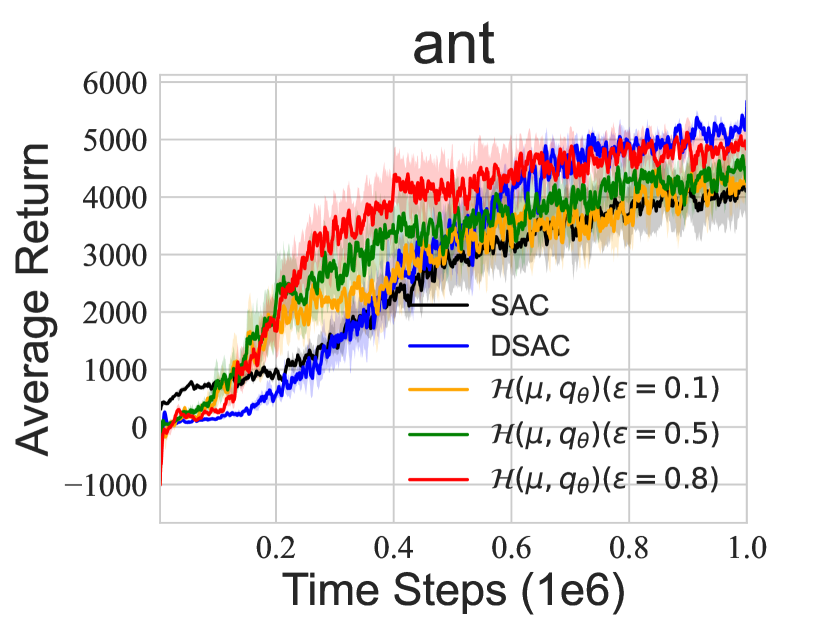
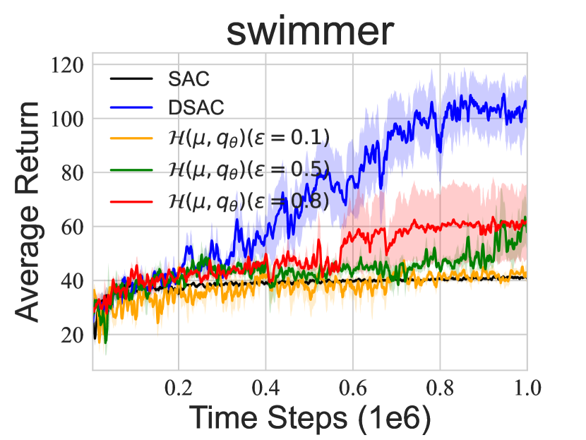
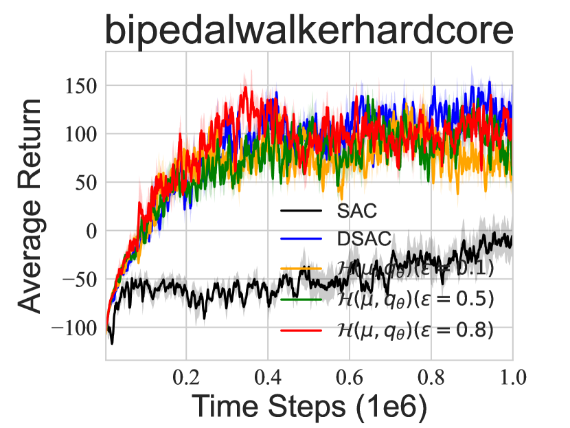
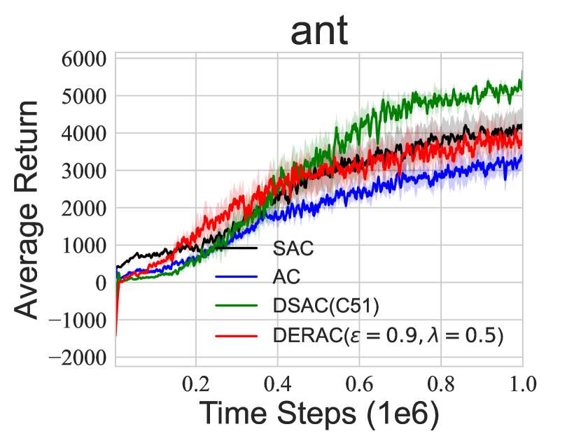
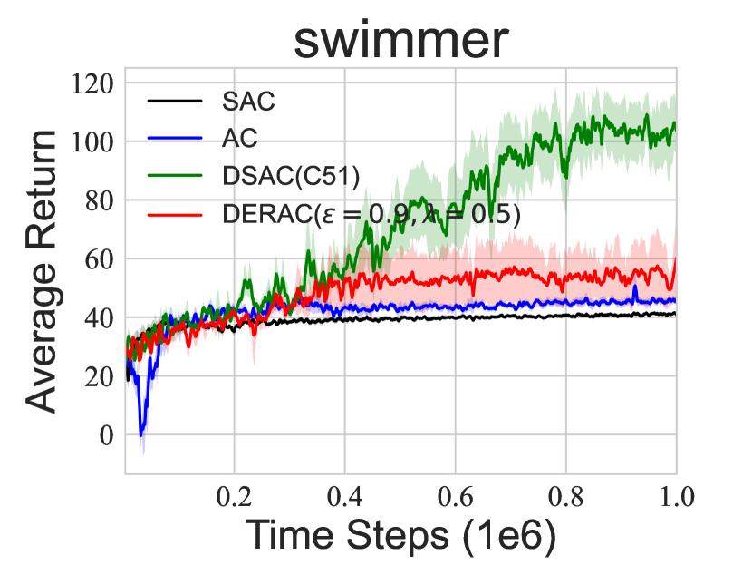
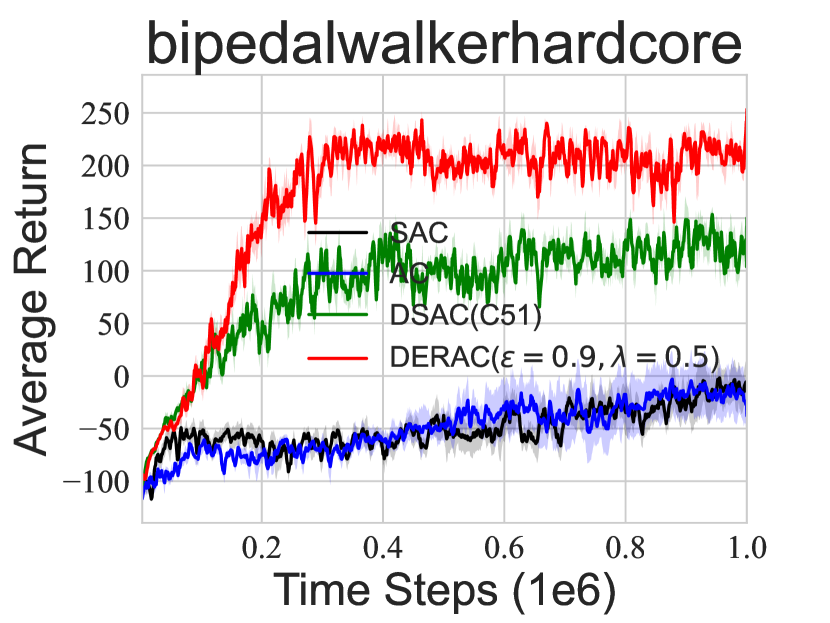
Figure 3: (First Row) Learning curves of Distributional AC (C51) with the return distribution decomposition $\mathcal{H}(\mu,q_{\theta})$ under different $\varepsilon$. (Second Row) Learning curves of DERAC algorithm. All results are averaged over five seeds. The AC baseline is without the leverage of entropy regularization.

6.1 Uncertainty-aware Regularization in Value-based Distributional RL

We demonstrate the rationale of action-state return density function decomposition in Eq. 3 and the uncertainty-aware entropy regularization effect analyzed in Eq. 4 based on the C51 algorithm. Firstly, the return distribution decomposition is based on the equivalence between KL divergence and cross-entropy owing to the usage of target networks. As such, we demonstrate that the C51 algorithm can still achieve similar results under the cross-entropy loss across both Atari games and MuJoCo environments in Figure 5 of Appendix L. In the value-based C51 loss, we replace the whole target categorical distribution $\widehat{p}^{s,a}(x)$ in C51 with the derived $\widehat{\mu}^{s,a}(x)$ under different $\varepsilon$ based on Eq. 3 in the cross-entropy loss, allowing us to investigate the uncertainty-aware regularization effect of distributional RL. Concretely, we define $\varepsilon$ as the proportion of probability of the bin that contains the expectation with mass to be transported to other bins. We use $\varepsilon$ to replace $\epsilon$ for convenience as the leverage of $\varepsilon$ can always guarantee the valid density function $\widehat{\mu}$ analyzed in Proposition 4.1. A significant proportion probability $\varepsilon$ that transports less mass to other bins corresponds to a large $\epsilon$ in Eq. 3, which would be closer to a distributional RL algorithm, i.e., C51.

As shown in Figure 2, when $\varepsilon$ gradually decreases from 0.8 to 0.1, learning curves of decomposed C51 denoted as $\mathcal{H}(\mu,q_{\theta})(\varepsilon=0.8/0.5/0.1)$ tend to degrade from vanilla C51 to DQN across most eight Atari games, and their sensitivity in terms of $\varepsilon$ may depend on the environment. This empirical observation corroborates the role of uncertainty-aware regularization we have derived in Section 4.2, suggesting that the uncertainty-aware entropy regularization is pivotal to the empirical success of CDRL.

6.2 Uncertainty-aware Regularization in Actor Critic

As suggested in the first row of Figure 3, the performance of the decomposed DSAC (C51), denoted as $\mathcal{H}(\mu,q_{\theta})(\varepsilon=0.8/0.5/0.1)$, also tends to vary from the vanilla DSAC (C51) to SAC with the decreasing of $\varepsilon$ on three MuJoCo environments, except bipedalwalkerhardcore. It is worth noting that our return density decomposition is valid only when $\epsilon\geq 1-p_{E}$ as shown in Proposition 4.1, and therefore $\epsilon$ can not strictly go to 0, where $\mathcal{H}(\mu,q_{\theta})$ would degenerate to SAC ideally.

The second row of Figure 3 showcases that DERAC (the red line) tends to “interpolate” between the expectation-based AC (without vanilla entropy) / SAC and DSAC (C51) across three MuJoCo environments, except bipedalwalkerhardcore (hard for exploration), where the interpolation has extra advantages. We hypothesize that our derived regularization improves the performance on complicated environments, e.g., bipedalwalkerhardcore, for which we provide more results and discussions in Appendix M.

We emphasize that introducing the DERAC algorithm is not to pursue the empirical outperformance over DSAC but to corroborate the rationale of incorporating uncertainty-aware regularization in actor-critic framework. Observing the interpolating behavior of DERAC between SAC and DSAC also substantiates the theoretical convergence of the tabular DERPI algorithm in Theorem 5.2. Specifically, as we choose $\varepsilon=0.9$ in DERAC, a distribution information loss exists, resulting in the learning performance degradation, e.g., on Swimmer. To pursue the performance in practice, our suggestion is to directly deploy DSAC that takes advantage of the full return distribution information in the learning. We also provide a sensitivity analysis of DERAC regarding $\lambda$ in Figure 6 of Appendix L.

6.3 Mutual Impacts of Vanilla Entropy Regularization and Uncertainty-aware Regularization

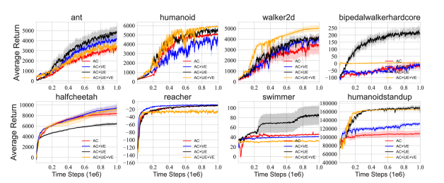
Figure 4: Learning curves of AC, AC+VE (SAC), AC+UE and AC+UE+VE (DSAC) over five seeds with smooth size five across eight MuJoCo environments where distributional RL is based on IQN.

Since the implicit regularization we reveal is highly linked to CDRL, we study the mutual impacts of explicit regularization in SAC and implicit regularization in DSAC in quantile-based distributional RL, e.g., QR-DQN (Dabney et al., 2018b) to reveal that the impact regularization in CDRL potentially exists in the general distributional RL. Similar results conducted on DSAC (C51) are also given in Appendix N. Specifically, we conduct a careful ablation study to control the effects of vanilla entropy (VE), uncertainty-aware entropy (UE), and their mutual impacts. We denote SAC with and without vanilla entropy as AC+VE and AC, and distributional SAC with and without vanilla entropy as AC+UE+VE and AC+UE, where VE and UE are short for Vanilla Entropy and Uncertainty-aware Entropy. For the implementation, we leverage the quantiles generation strategy in IQN (Dabney et al., 2018a) in distributional SAC (Ma et al., 2020). Hyper-parameters are listed in Appendix J.

As shown in Figure 4, an interesting observation is that the uncertainty-aware and vanilla entropy regularization may interfere with each other, e.g., on BipealWalkerHardcore and Swimmer, where AC+UE+VE (orange lines) is significantly inferior to AC+UE (black lines). This may result from the different exploration preferences in the policy learning for the two regularization. SAC explicitly optimizes the policy to visit states with high entropy, while distributional RL implicitly optimizes the policy to visit states and the following actions whose current return distribution estimate lags far behind the environment uncertainty. We hypothesize that mixing two different policy optimization/exploration directions may lead to sub-optimal solutions in certain environments, degrading the performance under this interference.

7 Discussions and Conclusion

The uncertainty-aware regularization with the exploration effect we reveal is mainly based on CDRL. Although CDRL is viewed as the first successful distributional RL family, the theoretical techniques, including the contraction analysis, in other distributional RL families, e.g., QR-DQN, are highly different from CDRL (Rowland et al., 2023a). As such, theoretical gaps remain to extend the uncertainty-aware exploration result in CDRL to general distributional RL algorithms, which we leave as future work.

In this paper, we interpret the potential superiority of CDRL over expectation-based RL as the uncertainty-aware regularization derived through the return density decomposition. In contrast to the explicit policy optimization in MaxEnt RL, the uncertainty-aware regularization in CDRL serves as an augmented reward, which implicitly optimizes the policy for an uncertainty-aware exploration. Starting from CDRL, our research contributes to a deeper understanding of the potential superiority of distributional RL algorithms.

Impact Statements

This paper presents work whose goal is to advance the field of Machine Learning. There are many potential societal consequences of our work, none of which we feel must be specifically highlighted here.

Appendix A Convergence Guarantee of Categorical Distributional RL

Categorical Distributional RL (Bellemare et al., 2017a) uses the heuristic projection operator $\Pi_{\mathcal{C}}$ that was defined as

$$\Pi_{\mathcal{C}}\left(\delta_{y}\right)=\left\{\begin{array}[]{ll}\delta_{l_{1}}&y\leq l_{1}\\ \frac{l_{i+1}-y}{l_{i+1}-z_{i}}\delta_{l_{i}}+\frac{y-l_{i}}{l_{i+1}-z_{i}}\delta_{l_{i+1}}&l_{i}<y\leq l_{i+1}\\ \delta_{l_{K}}&y>l_{K}\end{array},\right.$$ (11)

and extended affinely to finite mixtures of Dirac measures, so that for a mixture of Diracs $\sum_{i=1}^{N}p_{i}\delta_{y_{i}}$, we have $\Pi_{\mathcal{C}}\left(\sum_{i=1}^{N}p_{i}\delta_{y_{i}}\right)=\sum_{i=1}^{N}p_{i}\Pi_{\mathcal{C}}\left(\delta_{y_{i}}\right)$. The Cramér distance was recently studied as an alternative to the Wasserstein distances in the context of generative models (Bellemare et al., 2017b). Recall the definition of Cramér distance.

Definition 1.

(Definition 3 (Rowland et al., 2018)) The Cramér distance $\ell_{2}$ between two distributions $\nu_{1},\nu_{2}\in\mathscr{P}(\mathbb{R})$, with cumulative distribution functions $F_{\nu_{1}},F_{\nu_{2}}$ respectively, is defined by:

$$\ell_{2}\left(\nu_{1},\nu_{2}\right)=\left(\int_{\mathbb{R}}\left(F_{\nu_{1}}(x)-F_{\nu_{2}}(x)\right)^{2}\mathrm{~{}d}x\right)^{1/2}.$$

Further, the supremum-Cramér metric $\bar{\ell}_{2}$ is defined between two distribution functions $\eta,\mu\in\mathscr{P}(\mathbb{R})^{\mathcal{X}\times\mathcal{A}}$ by

$$\bar{\ell}_{2}(\eta,\mu)=\sup_{(x,a)\in\mathcal{X}\times\mathcal{A}}\ell_{2}\left(\eta^{(x,a)},\mu^{(x,a)}\right).$$

Thus, the contraction of categorical distributional RL can be guaranteed under Cramér distance:

Proposition A.1.

(Proposition 2 (Rowland et al., 2018)) The operator $\Pi_{\mathcal{C}}\mathcal{T}^{\pi}$ is a $\sqrt{\gamma}$-contraction in $\bar{\ell}_{2}$.

An insight behind this conclusion is that Cramér distance endows a particular subset with a notion of orthogonal projection, and the orthogonal projection onto the subset is exactly the heuristic projection $\Pi_{\mathcal{C}}$ (Proposition 1 in (Rowland et al., 2018)).

Appendix B Proof of Proposition 4.1

Proposition 4.1. Denote $\widehat{p}^{s,a}(x\in\Delta_{E})=p_{E}/\Delta$. Following the density function decomposition in Eq. 3, $\widehat{\mu}(x)=\sum_{i=1}^{N}p^{\mu}_{i}\mathds{1}(x\in\Delta_{i})/\Delta$ is a valid probability density function if and only if $\epsilon\geq 1-p_{E}$.

Proof.

Recap a valid probability density function requires non-negative and one-bounded probability in each bin and all probabilities should sum to 1.

Necessity. (1) When $x\in\Delta_{E}$, Eq. 3 can simplified as $p_{E}/\Delta=(1-\epsilon)/\Delta+\epsilon p_{E}^{\mu}/\Delta$, where $p_{E}^{\mu}=\widehat{\mu}(x\in\Delta_{E})$. Thus, $p_{E}^{\mu}=\frac{p_{E}}{\epsilon}-\frac{1-\epsilon}{\epsilon}\geq 0$ if $\epsilon\geq 1-p_{E}$. Obviously, $p_{E}^{\mu}=\frac{p_{E}}{\epsilon}-\frac{1-\epsilon}{\epsilon}\leq\frac{1}{\epsilon}-\frac{1-\epsilon}{\epsilon}=1$ guaranteed by the validity of $\widehat{p}^{s,a}_{E}$. (2) When $x\notin\Delta_{E}$, we have $p_{i}/\Delta=\epsilon p_{i}^{\mu}/\Delta$, i.e.,When $x\notin\Delta_{E}$, We immediately have $p^{\mu}_{i}=\frac{p_{i}}{\epsilon}\leq\frac{1-p_{E}}{\epsilon}\leq 1$ when $\epsilon\geq 1-p_{E}$. Also, $p^{\mu}_{i}=\frac{p_{i}}{\epsilon}\geq 0$.

Sufficiency. (1) When $x\in\Delta_{E}$, let $p_{E}^{\mu}=\frac{p_{E}}{\epsilon}-\frac{1-\epsilon}{\epsilon}\geq 0$, we have $\epsilon\geq 1-p_{E}$. $p_{E}^{\mu}=\frac{p_{E}}{\epsilon}-\frac{1-\epsilon}{\epsilon}\leq 1$ in nature. (2) When $x\notin\Delta_{E}$, $p^{\mu}_{i}=\frac{p_{i}}{\epsilon}\geq 0$ in nature. Let $p^{\mu}_{i}=\frac{p_{i}}{\epsilon}\leq 1$, we have $p_{i}\leq\epsilon$. We need to take the intersection set of (1) and (2), and we find that $\epsilon\geq 1-p_{E}\Rightarrow\epsilon\geq 1-p_{E}\geq p_{i}$ that satisfies the condition in (2). Thus, the intersection set of (1) and (2) would be $\epsilon\geq 1-p_{E}$.

In summary, as $\epsilon\geq 1-p_{E}$ is both the necessary and sufficient condition, we have the conclusion that $\widehat{\mu}(x)$ is a valid probability density function $\iff\epsilon\geq 1-p_{E}$.

∎

Appendix C Equivalence between Categorical and Histogram Parameterization

Proposition C.1.

Suppose the target categorical distribution $c=\sum_{i=1}^{N}p_{i}\delta_{z_{i}}$ and the target histogram function $h(x)=\sum_{i=1}^{N}p_{i}\mathds{1}(x\in\Delta_{i})/\Delta$, updating the parameterized categorical distribution $c_{\theta}$ under KL divergence is equivalent to updating the parameterized histogram function $h_{\theta}$.

Proof.

For the histogram density estimator $h_{\theta}$ and the true target density function $p(x)$, we can simplify the KL divergence as follows.

$$D_{\text{KL}}(h,h_{\theta}) =\sum_{i=1}^{N}\int_{l_{i-1}}^{l_{i}}\frac{p_{i}(x)}{\Delta}\log\frac{\frac{p_{i}(x)}{\Delta}}{\frac{h^{i}_{\theta}}{\Delta}}dx$$ (12)

$$=\sum_{i=1}^{N}\int_{l_{i-1}}^{l_{i}}\frac{p_{i}(x)}{\Delta}\log\frac{p_{i}(x)}{\Delta}dx-\sum_{i=1}^{N}\int_{l_{i-1}}^{l_{i}}\frac{p_{i}(x)}{\Delta}\log\frac{h^{i}_{\theta}}{\Delta}dx$$

$$\propto-\sum_{i=1}^{N}\int_{l_{i-1}}^{l_{i}}\frac{p_{i}(x)}{\Delta}\log\frac{h^{i}_{\theta}}{\Delta}dx$$

$$=-\sum_{i=1}^{N}p_{i}(x)\log\frac{h^{i}_{\theta}}{\Delta}\propto-\sum_{i=1}^{N}p_{i}(x)\log h_{\theta}^{i}$$

where $h^{i}_{\theta}$ is determined by $i$ and $\theta$ and is independent of $x$. For categorical distribution estimator $c_{\theta}$ with the probability $p_{i}$ in for each atom $z_{i}$, we also have its target categorical distribution $p(x)$ with each probability $p_{i}$, we have:

$$D_{\text{KL}}(c,c_{\theta})=\sum_{i=1}^{N}p_{i}\log\frac{p_{i}}{c_{\theta}^{i}}=\sum_{i=1}^{N}p_{i}\log p_{i}-\sum_{i=1}^{N}p_{i}\log c_{\theta}^{i}\propto-\sum_{i=1}^{N}p_{i}\log c_{\theta}^{i}$$ (13)

∎

In CDRL, we only use a discrete categorical distribution with probabilities centered on the fixed atoms $\{z_{i}\}_{i=1}^{N}$, while the histogram density estimator in our analysis is a continuous function defined on $[z_{0},z_{N}]$ to allow richer analysis. We reveal that minimizing the KL divergence regarding the parameterized categorical distribution in Eq. 13 is equivalent to minimizing the cross-entropy loss regarding the parameterized histogram function in Eq. 12.

Appendix D Theoretical Results about Histogram Density Estimator in Distributional RL

Histogram Function Parameterization Error: Uniform Convergence in Probability. The previous discrete categorical parameterization error bound in (Rowland et al., 2018) (Proposition 3) is derived between the true return distribution and the limiting return distribution denoted as $\eta_{\mathcal{C}}$ iteratively updated via the Bellman operator $\Pi_{\mathcal{C}}\mathfrak{T}^{\pi}$ in expectation, without considering an asymptotic analysis when the number of sampled $\{s_{i},a_{i}\}_{i=1}^{n}$ pairs goes to infinity. As a complementary result, we provide a uniform convergence rate for the histogram density estimator in the context of distributional RL. In this particular analysis within this subsection, we denote $\widehat{p}^{s,a}_{\mathcal{C}}$ as the density function estimator for the true limiting return distribution $\eta_{\mathcal{C}}$ via $\Pi_{\mathcal{C}}\mathfrak{T}^{\pi}$ with its true density ${p}^{s,a}_{\mathcal{C}}$. In Theorem D.1, we show that the sample-based histogram estimator $\widehat{p}^{s,a}_{\mathcal{C}}$ can approximate any arbitrary continuous limiting density function $p^{s,a}_{\mathcal{C}}$ under a mild condition.

Theorem D.1.

(Uniform Convergence Rate in Probability) Suppose $p^{s,a}_{\mathcal{C}}(x)$ is Lipschitz continuous and the support of a random variable is partitioned by N bins with bin size $\Delta$. Then

$$\sup_{x}\left|\widehat{p}^{s,a}_{\mathcal{C}}(x)-p^{s,a}_{\mathcal{C}}(x)\right|=O\left(\Delta\right)+O_{P}\left(\sqrt{\frac{\log N}{n\Delta^{2}}}\right).$$ (14)

Proof.

Our proof is mainly based on the non-parametric statistics analysis  (Wasserman, 2006). In particular, the difference of $\widehat{p}^{s,a}_{\mathcal{C}}(x)-p_{\mathcal{C}}^{s,a}(x)$ can be written as

$$\widehat{p}^{s,a}_{\mathcal{C}}(x)-p^{s,a}_{\mathcal{C}}(x)=\underbrace{\mathbb{E}\left(\widehat{p}^{s,a}_{\mathcal{C}}(x)\right)-p^{s,a}_{\mathcal{C}}(x)}_{\text{bias }}+\underbrace{\widehat{p}^{s,a}_{\mathcal{C}}(x)-\mathbb{E}\left(\widehat{p}^{s,a}_{\mathcal{C}}(x)\right)}_{\text{stochastic variation }}.$$ (15)

(1) The first bias term. Without loss of generality, we consider $x\in\Delta_{k}$, we have

$$\mathbb{E}\left(\widehat{p}^{s,a}_{\mathcal{C}}(x)\right) =\frac{P(X\in\Delta_{k})}{\Delta}$$ (16)

$$=\frac{\int_{l_{0}+(k-1)\Delta}^{l_{0}+k\Delta}p(y)dy}{\Delta}$$

$$=\frac{F(l_{0}+(k-1)\Delta)-F(l_{0}+(k-1)\Delta)}{l_{0}+k\Delta-(l_{0}+(k-1)\Delta)}$$

$$=p^{s,a}_{\mathcal{C}}(x^{\prime}),$$

where the last equality is based on the mean value theorem. According to the L-Lipschitz continuity property, we have

$$|\mathbb{E}\left(\widehat{p}^{s,a}_{\mathcal{C}}(x)\right)-p^{s,a}_{\mathcal{C}}(x)|=|p^{s,a}_{\mathcal{C}}(x^{\prime})-p^{s,a}_{\mathcal{C}}(x)|\leq L|x^{\prime}-x|\leq L\Delta$$ (17)

(2) The second stochastic variation term. If we let $x\in\Delta_{k}$, then $\widehat{p}^{s,a}_{\mathcal{C}}=p_{k}=\frac{1}{n}\sum_{i=1}^{n}\mathds{1}(X_{i}\in\Delta_{k})$, we thus have

$$P\left(\sup_{x}\left|\widehat{p}^{s,a}_{\mathcal{C}}(x)-\mathbb{E}\left(\widehat{p}^{s,a}_{\mathcal{C}}(x)\right)\right|>\epsilon\right)$$ (18)

$$=P\left(\max_{j=1,\cdots,N}\left|\frac{1}{n}\sum_{i=1}^{n}\mathds{1}\left(X_{i}\in\Delta_{j}\right)/\Delta-P\left(X_{i}\in\Delta_{j}\right)/\Delta\right|>\epsilon\right)$$

$$=P\left(\max_{j=1,\cdots,N}\left|\frac{1}{n}\sum_{i=1}^{n}\mathds{1}\left(X_{i}\in\Delta_{j}\right)-P\left(X_{i}\in\Delta_{j}\right)\right|>\Delta\epsilon\right)$$

$$\leq\sum_{j=1}^{N}P\left(\left|\frac{1}{n}\sum_{i=1}^{n}\mathds{1}\left(X_{i}\in\Delta_{j}\right)-P\left(X_{i}\in\Delta_{j}\right)\right|>\Delta\epsilon\right)$$

$$\leq N\cdot\exp\left(-2n\Delta^{2}\epsilon^{2}\right)\quad\text{(by Hoeffding’s inequality)},$$

where in the last inequality we know that the indicator function is bounded in [0, 1]. We then let the last term be a constant independent of $N,n,\Delta$ and simplify the order of $\epsilon$. Then, we have:

$$\sup_{x}\left|\widehat{p}^{s,a}_{\mathcal{C}}(x)-\mathbb{E}\left(\widehat{p}^{s,a}_{\mathcal{C}}(x)\right)\right|=O_{P}\left(\sqrt{\frac{\log N}{n\Delta^{2}}}\right)$$ (19)

In summary, as the above inequality holds for each $x$, we thus have the uniform convergence rate of a histogram density estimator

$$\begin{aligned} \sup_{x}\left|\widehat{p}^{s,a}_{\mathcal{C}}(x)-p^{s,a}_{\mathcal{C}}(x)\right|&\leq\sup_{x}\left|\mathbb{E}\left(\widehat{p}^{s,a}_{\mathcal{C}}(x)\right)-p^{s,a}_{\mathcal{C}}(x)\right|+\sup_{x}\left|\widehat{p}^{s,a}_{\mathcal{C}}(x)-\mathbb{E}\left(\widehat{p}^{s,a}_{\mathcal{C}}(x)\right)\right|\\ &=O\left(\Delta\right)+O_{P}\left(\sqrt{\frac{\log N}{n\Delta^{2}}}\right).\end{aligned}$$ (20)

∎

Appendix E Discussion about KL Divergence in Distributional RL

Remark on KL Divergence. As stated in Section 3 of CDRL (Bellemare et al., 2017a), when the categorical parameterization is applied after the projection operator $\Pi_{\mathcal{C}}$, the distributional Bellman operator $\mathfrak{T}^{\pi}$ has the contraction guarantee under Cramér distance (Rowland et al., 2018), albeit the use of a non-expansive KL divergence (Morimura et al., 2012). Similarly, our histogram density parameterization with the projection $\Pi_{\mathcal{C}}$ and KL divergence also enjoys a contraction property due to the equivalence between optimizing histogram function and categorical distribution analyzed in Appendix C. We summarize favorable properties of KL divergence in distributional RL as follows.

Proposition E.1.

Given two probability measures $\mu$ and $\nu$, we define the supreme $D_{\text{KL}}$ as a functional $\mathcal{P}(\mathcal{X})^{\mathcal{S}\times\mathcal{A}}\times\mathcal{P}(\mathcal{X})^{\mathcal{S}\times\mathcal{A}}\rightarrow\mathbb{R}$, i.e., $D_{\text{KL}}^{\infty}(\mu,\nu)=\sup_{(x,a)\in\mathcal{S}\times\mathcal{A}}D_{\text{KL}}(\mu(x,a),\nu(x,a))$. we have: (1) $\mathfrak{T}^{\pi}$ is a non-expansive distributional Bellman operator under $D_{\text{KL}}^{\infty}$, i.e., $D_{\text{KL}}^{\infty}(\mathfrak{T}^{\pi}Z_{1},\mathfrak{T}^{\pi}Z_{2})\leq D_{\text{KL}}^{\infty}(Z_{1},Z_{2})$, (2) $D_{\text{KL}}^{\infty}(Z_{n},Z)\rightarrow 0$ implies the Wasserstein distance $W_{p}(Z_{n},Z)\rightarrow 0$, (3) the expectation of $Z^{\pi}$ is still $\gamma$-contractive under $D_{\text{KL}}^{\infty}$, i.e., $\left\|\mathbb{E}\mathfrak{T}^{\pi}Z_{1}-\mathbb{E}\mathfrak{T}^{\pi}Z_{2}\right\|_{\infty}\leq\gamma\left\|\mathbb{E}Z_{1}-\mathbb{E}Z_{2}\right\|_{\infty}$.

Proof.

We firstly assume $Z_{\theta}$ is absolutely continuous and the supports of two distributions in KL divergence have a negligible intersection (Arjovsky & Bottou, 2017), under which the KL divergence is well-defined.

(1) Please refer to (Morimura et al., 2012) for the proof. Therefore, we have $D_{\text{KL}}^{\infty}(\mathfrak{T}^{\pi}Z_{1},\mathfrak{T}^{\pi}Z_{2})\leq D_{\text{KL}}^{\infty}(Z_{1},Z_{2})$, implying that $\mathfrak{T}^{\pi}$ is a non-expansive operator under $D_{\text{KL}}^{\infty}$.

(2) By the definition of $D_{\text{KL}}^{\infty}$, we have $\sup_{s,a}D_{\text{KL}}(Z_{n}(s,a),Z(s,a))\rightarrow 0$ implies $D_{\text{KL}}(Z_{n},Z)\rightarrow 0$. $D_{\text{KL}}(Z_{n},Z)\rightarrow 0$ implies the total variation distance $\delta(Z_{n},Z)\rightarrow 0$ according to a straightforward application of Pinsker’s inequality

$$\delta\left(Z_{n},Z\right)\leq\sqrt{\frac{1}{2}D_{\text{KL}}\left(Z_{n},Z\right)}\rightarrow 0$$ (21)

$$\delta\left(Z,Z_{n}\right)\leq\sqrt{\frac{1}{2}D_{\text{KL}}\left(Z,Z_{n}\right)}\rightarrow 0$$

Based on Theorem 2 in WGAN (Arjovsky et al., 2017), $\delta(Z_{n},Z)\rightarrow 0$ implies $W_{p}(Z_{n},Z)\rightarrow 0$. This is trivial by recalling the fact that $\delta$ and $W$ give the strong and weak topologies on the dual of $(C(\mathcal{X}),\|\cdot\|_{\infty})$ when restricted to $\text{Prob}(\mathcal{X})$.

(3) The conclusion holds because the $\mathfrak{T}^{\pi}$ degenerates to $\mathcal{T}^{\pi}$ regardless of the metric $d_{p}$ (Bellemare et al., 2017a). Specifically, due to the linearity of expectation, we obtain that

$$\left\|\mathbb{E}\mathfrak{T}^{\pi}Z_{1}-\mathbb{E}\mathfrak{T}^{\pi}Z_{2}\right\|_{\infty}=\left\|\mathcal{T}^{\pi}\mathbb{E}Z_{1}-\mathcal{T}^{\pi}\mathbb{E}Z_{2}\right\|_{\infty}\leq\gamma\|\mathbb{E}Z_{1}-\mathbb{E}Z_{2}\|_{\infty}.$$ (22)

This implies that the expectation of $Z$ under $D_{\text{KL}}$ exponentially converges to the expectation of $Z^{*}$, i.e., $\gamma$-contraction. ∎

Appendix F Proof of Proposition 4.2

Proposition 4.2 (Decomposed Neural FZI) Denote $q_{\theta}^{s,a}(x)$ as the histogram density function of $Z^{k}_{\theta}(s,a)$ in Neural FZI. Based on Eq. 3 and KL divergence as $d_{p}$, Neural FZI in Eq. 2 is simplified as

$${Z}_{\theta}^{k+1}=\underset{q_{\theta}}{\operatorname{argmin}}\frac{1}{n}\sum_{i=1}^{n}[\underset{(a)}{\underbrace{-\log q^{s_{i},a_{i}}_{\theta}(\Delta^{i}_{E})}}+\alpha\mathcal{H}(\widehat{\mu}^{s_{i}^{\prime},\pi_{Z}(s^{\prime}_{i})},q^{s_{i},a_{i}}_{\theta})],$$ (23)

Proof.

Firstly, given a fixed $p(x)$ we know that minimizing $D_{\text{KL}}(p,q_{\theta})$ is equivalent to minimizing $\mathcal{H}(p,q)$ by following

$$D_{\text{KL}}(p,q_{\theta}) =\sum_{i=1}^{N}\int_{l_{i-1}}^{l_{i}}p_{i}(x)/\Delta\log\frac{p^{i}(x)/\Delta}{q^{i}_{\theta}/\Delta}\mathrm{~{}d}x$$ (24)

$$=-\sum_{i=1}^{N}\int_{l_{i-1}}^{l_{i}}p_{i}(x)/\Delta\log q^{i}_{\theta}/\Delta\mathrm{~{}d}x-(\sum_{i=1}^{N}\int_{l_{i-1}}^{l_{i}}p_{i}(x)/\Delta\log p^{i}(x)/\Delta\mathrm{~{}d}x)$$

$$=\mathcal{H}(p,q_{\theta})-\mathcal{H}(p)$$

$$\propto\mathcal{H}(p,q_{\theta})$$

where $p=\sum_{i=1}^{N}p_{i}(x)\mathds{1}(x\in\Delta^{i})/\Delta$ and $q_{\theta}=\sum_{i=1}^{N}q_{i}/\Delta$. Based on $\mathcal{H}(p,q_{\theta})$, we use $p^{s_{i}^{\prime},\pi_{Z}(s^{\prime}_{i})}(x)$ to denote the target probability density function of the random variable $R(s_{i},a_{i})+\gamma Z^{k}_{\theta^{*}}\left(s_{i}^{\prime},\pi_{Z}(s_{i}^{\prime})\right)$. Then, we can derive the objective function within each Neural FZI as

$$\frac{1}{n}\sum_{i=1}^{n}\mathcal{H}(p^{s_{i}^{\prime},\pi_{Z}(s^{\prime}_{i})}(x),q_{\theta}^{s_{i},a_{i}})$$ (25)

$$=\frac{1}{n}\sum_{i=1}^{n}\left((1-\epsilon)\mathcal{H}(\mathds{1}(x\in\Delta^{i}_{E})/\Delta,q_{\theta}^{s_{i},a_{i}})+\epsilon\mathcal{H}(\widehat{\mu}^{s_{i}^{\prime},\pi_{Z}(s^{\prime}_{i})},q_{\theta}^{s_{i},a_{i}})\right)$$

$$=\frac{1}{n}\sum_{i=1}^{n}\left(-(1-\epsilon)\sum_{j=1}^{N}\int_{l_{j-1}}^{l_{j}}\mathds{1}(x\in\Delta^{i}_{E})/\Delta\log q_{\theta}^{s_{i},a_{i}}(\Delta_{j})/\Delta dx-\epsilon\sum_{j=1}^{N}\int_{l_{j-1}}^{l_{j}}p^{\mu}_{j}/\Delta\log q_{\theta}^{s_{i},a_{i}}(\Delta_{j})/\Delta\right)$$

$$=\frac{1}{n}\sum_{i=1}^{n}\frac{1}{\Delta}\left((1-\epsilon)(-\log q_{\theta}^{s_{i},a_{i}}(\Delta^{i}_{E})/\Delta)-\epsilon\sum_{j=1}^{N}p^{\mu}_{j}\log q_{\theta}^{s_{i},a_{i}}(\Delta_{j})/\Delta\right)$$

$$\propto\frac{1}{n}\sum_{i=1}^{n}\left((1-\epsilon)(-\log q_{\theta}^{s_{i},a_{i}}(\Delta^{i}_{E}))+\epsilon\mathcal{H}(\widehat{\mu}^{s_{i}^{\prime},\pi_{Z}(s^{\prime}_{i})},q_{\theta}^{s_{i},a_{i}})\right)$$

$$\propto\frac{1}{n}\sum_{i=1}^{n}\left(-\log q_{\theta}^{s_{i},a_{i}}(\Delta^{i}_{E})+\alpha\mathcal{H}(\widehat{\mu}^{s_{i}^{\prime},\pi_{Z}(s^{\prime}_{i})},q_{\theta}^{s_{i},a_{i}})\right),\ \text{where}\ \alpha=\frac{\epsilon}{1-\epsilon}>0$$

where recall that $\widehat{\mu}^{s_{i}^{\prime},\pi_{Z}(s^{\prime}_{i})}=\sum_{i=1}^{N}p^{\mu}_{i}(x)\mathds{1}(x\in\Delta_{i})/\Delta=\sum_{i=1}^{N}p^{\mu}_{i}/\Delta$ for conciseness and denote $q^{s_{i},a_{i}}_{\theta}=\sum_{j=1}^{N}q^{s_{i},a_{i}}_{\theta}(\Delta_{j})/\Delta$. The cross-entropy $\mathcal{H}(\widehat{\mu}^{s_{i}^{\prime},\pi_{Z}(s^{\prime}_{i})},q_{\theta}^{s_{i},a_{i}})$ is based on the discrete distribution when $i=1,...,N$. $\Delta_{E}^{i}$ represent the interval that $\mathbb{E}\left[R(s_{i},a_{i})+\gamma Z^{k}_{\theta^{*}}\left(s_{i}^{\prime},\pi_{Z}(s_{i}^{\prime})\right)\right]$ falls into, i.e., $\mathbb{E}\left[R(s_{i},a_{i})+\gamma Z^{k}_{\theta^{*}}\left(s_{i}^{\prime},\pi_{Z}(s_{i}^{\prime})\right)\right]\in\Delta_{E}^{i}$. ∎

Appendix G Proof of Proposition 4.3

Proposition 4.3 (Equivalence between the term (a) in Decomposed Neural FZI and Neural FQI) In Eq. 4 of Neural FZI, assume the function class $\{Z_{\theta}:\theta\in\Theta\}$ is sufficiently large such that it contains the target $\{Y_{i}^{k}\}_{i=1}^{n}$, when $\Delta\rightarrow 0$, for all $k$, minimizing the term (a) in Eq. 4 implies

$$P(Z^{k+1}_{\theta}(s,a)=\mathcal{T}^{\text{opt}}Q^{k}_{\theta^{*}}(s,a))=1,\quad\text{and}\quad\int_{-\infty}^{+\infty}\left|F_{q_{\theta}}(x)-F_{\delta_{\mathcal{T}^{\text{opt}}Q^{k}_{\theta^{*}}(s,a)}}(x)\right|dx=o(\Delta),$$ (26)

where $\mathcal{T}^{\text{opt}}Q^{k}_{\theta^{*}}(s,a)$ is the scalar-valued target in the k-th phase of Neural FQI, and $\delta_{\mathcal{T}^{\text{opt}}Q^{k}_{\theta^{*}}(s,a)}$ is the Dirac delta function defined on the scalar $\mathcal{T}^{\text{opt}}Q^{k}_{\theta^{*}}(s,a)$.

Proof.

Firstly, we define the distributional Bellman optimality operator $\mathfrak{T}^{\text{opt}}$ as follows:

$$\mathfrak{T}^{\text{opt}}Z(s,a)\stackrel{{\scriptstyle D}}{{=}}R(s,a)+\gamma Z\left(S^{\prime},a^{*}\right),$$ (27)

where $S^{\prime}\sim P(\cdot\mid s,a)$ and $a^{*}=\underset{a^{\prime}}{\operatorname{argmax}}\mathbb{E}\left[Z\left(S^{\prime},a^{\prime}\right)\right]$. If $\{Z_{\theta}:\theta\in\Theta\}$ is sufficiently large enough such that it contains $\mathfrak{T}^{\text{opt}}Z_{\theta^{*}}$ ($\{Y_{i}^{k}\}_{i=1}^{n}$), then optimizing Neural FZI in Eq. 2 leads to $Z_{\theta}^{k+1}=\mathfrak{T}^{\text{opt}}Z_{\theta^{*}}$.

Secondly, we apply the action-value density function decomposition on the target histogram function $\widehat{p}^{s,a}(x)$. Consider the parameterized histogram density function $h_{\theta}$ and denote $h^{E}_{\theta}/\Delta$ as the bin height in the bin $\Delta_{E}$, under the KL divergence between the first histogram function $\mathds{1}(x\in\Delta_{E})$ with $h_{\theta}(x)$, the objective function is simplified as

$$D_{\text{KL}}(\mathds{1}(x\in\Delta_{E})/\Delta,h_{\theta}(x)) =-\int_{x\in\Delta_{E}}\frac{1}{\Delta}\log\frac{\frac{h_{\theta}^{E}}{\Delta}}{\frac{1}{\Delta}}dx =-\log h_{\theta}^{E}$$ (28)

Since $\{Z_{\theta}:\theta\in\Theta\}$ is sufficiently large enough that can represent the pdf of $\{Y_{i}^{k}\}_{i=1}^{n}$, it also implies that $\{Z_{\theta}:\theta\in\Theta\}$ can represent the term (a) part in its pdf via the return density decomposition. The KL minimizer would be $\widehat{h}_{\theta}=\mathds{1}(x\in\Delta_{E})/\Delta$ in expectation. Then, $\lim_{\Delta\rightarrow 0}\arg\min_{h_{\theta}}D_{\text{KL}}(\mathds{1}(x\in\Delta_{E})/\Delta,h_{\theta}(x))=\delta_{\mathbb{E}\left[Z^{\text{target}}(s,a)\right]}$, where $\delta_{\mathbb{E}\left[Z^{\text{target}}(s,a)\right]}$ is a Dirac Delta function centered at $\mathbb{E}\left[Z^{\text{target}}(s,a)\right]$ and can be viewed as a generalized probability density function. That being said, the limiting probability density function (pdf) converges to a Dirac delta function at $\mathbb{E}\left[Z^{\text{target}}(s,a)\right]$. The limit behavior from a histogram function $\widehat{p}$ to a continuous one for $Z^{\text{target}}$ is guaranteed by Theorem D.1, and this also applies from $h_{\theta}$ to $Z_{\theta}$. In Neural FZI, we have $Z^{\text{target}}=\mathfrak{T}^{\text{opt}}Z_{\theta^{*}}$. Since here we use $Z^{k+1}_{\theta}(s,a)$ as the random variable who cdf is the limiting distribution, according to the definition of the Dirac function, as $\Delta\rightarrow 0$, we attain

$$P(Z^{k+1}_{\theta}(s,a)=\mathbb{E}\left[\mathfrak{T}^{\text{opt}}Z^{k}_{\theta^{*}}(s,a)\right])=1,$$ (29)

which is because if the pdf of a random variable is a Dirac delta function, it implies that the random variable takes this constant value with probability one. Due to the linearity of expectation in Lemma 4 of (Bellemare et al., 2017a), we have

$$\mathbb{E}\left[\mathfrak{T}^{\text{opt}}Z^{k}_{\theta^{*}}(s,a)\right]=\mathfrak{T}^{\text{opt}}\mathbb{E}\left[Z^{k}_{\theta^{*}}(s,a)\right]=\mathcal{T}^{\text{opt}}Q^{k}_{\theta^{*}}(s,a)$$ (30)

Finally, we obtain:

$$P(Z^{k+1}_{\theta}(s,a)=\mathcal{T}^{\text{opt}}Q^{k}_{\theta^{*}}(s,a))=1\quad\text{as}\ \ \Delta\rightarrow 0$$ (31)

In order to characterize how the difference varies when $\Delta\rightarrow 0$, we further define $\Delta_{E}=\left[l_{e},l_{e+1}\right)$ and we have:

$$\int_{-\infty}^{+\infty}\left|F_{q_{\theta}}(x)-F_{\delta_{\mathcal{T}^{\text{opt}}Q^{k}_{\theta^{*}}(s,a)}}(x)\right|dx =\frac{1}{2\Delta}\left(\left(\mathcal{T}^{\text{opt}}Q^{k}_{\theta^{*}}(s,a)-l_{e}\right)^{2}+\left(l_{e+1}-\mathcal{T}^{\text{opt}}Q^{k}_{\theta^{*}}(s,a)\right)^{2}\right)$$ (32)

$$=\frac{1}{2\Delta}(a^{2}+(\Delta-a)^{2})$$

$$\leq\Delta/2$$

$$=o(\Delta),$$

where $\mathcal{T}^{\text{opt}}Q^{k}_{\theta^{*}}(s,a)=\mathbb{E}\left[\mathfrak{T}^{\text{opt}}Z^{k}_{\theta^{*}}(s,a)\right]\in\Delta_{E}$ and we denote $a=\mathcal{T}^{\text{opt}}Q^{k}_{\theta^{*}}(s,a)-l_{e}$. The first equality holds as $q_{\theta}(x)$, the KL minimizer while minimizing the term (a), would follows a uniform distribution on $\Delta_{E}$, i.e., $\widehat{q}_{\theta}=\mathds{1}(x\in\Delta_{E})/\Delta$. Thus, the integral of LHS would be the area of two centralized triangles according. The inequality is because the maximizer is obtained when $a=\Delta$ or $0$. The result implies that the convergence rate in distribution difference is $o(\Delta)$.

∎

Appendix H Convergence Proof of DERPI in Theorem 5.2

H.1 Proof of Distribution-Entropy-Regularized Policy Evaluation in Lemma 5.1

Lemma 5.1(Distribution-Entropy-Regularized Policy Evaluation) Consider the distribution-entropy-regularized Bellman operator $\mathcal{T}_{d}^{\pi}$ in Eq. 7 and assume $\mathcal{H}(\mu^{s_{t},a_{t}},q_{\theta}^{s_{t},a_{t}})$ is bounded for all $(s_{t},a_{t})\in\mathcal{S}\times\mathcal{A}$. Define $Q^{k+1}=\mathcal{T}_{d}^{\pi}Q^{k}$, then $Q^{k+1}$ will converge to a corrected Q-value of $\pi$ as $k\rightarrow\infty$ with the new objective function $J^{\prime}(\pi)$ defined as

$$J^{\prime}(\pi)=\sum_{t=0}^{T}\mathbb{E}_{\left({s}_{t},{a}_{t}\right)\sim\rho_{\pi}}\left[r\left({s}_{t},{a}_{t}\right)+\gamma f(\mathcal{H}\left(\mu^{s_{t},a_{t}},q_{\theta}^{s_{t},a_{t}}\right))\right].$$ (33)

Proof.

Firstly, we plug in $V(s_{t+1})$ into RHS of the iteration in Eq. 7, then we obtain

$$\mathcal{T}_{d}^{\pi}Q\left({s}_{t},{a}_{t}\right)$$ (34)

$$=r\left({s}_{t},{a}_{t}\right)+\gamma\mathbb{E}_{{s}_{t+1}\sim P(\cdot|s_{t},a_{t})}\left[V\left({s}_{t+1}\right)\right]$$

$$=r\left({s}_{t},{a}_{t}\right)+\gamma f(\mathcal{H}\left(\mu^{s_{t},a_{t}},q_{\theta}^{s_{t},a_{t}}\right))+\gamma\mathbb{E}_{({s}_{t+1},a_{t+1})\sim\rho^{\pi}}\left[Q\left({s}_{t+1},{a}_{t+1}\right)\right]$$

$$\triangleq r_{\pi}\left({s}_{t},{a}_{t}\right)+\gamma\mathbb{E}_{({s}_{t+1},a_{t+1})\sim\rho^{\pi}}\left[Q\left({s}_{t+1},{a}_{t+1}\right)\right],$$

where $r_{\pi}\left({s}_{t},{a}_{t}\right)\triangleq r\left({s}_{t},{a}_{t}\right)+\gamma f(\mathcal{H}\left(\mu^{s_{t},a_{t}},q_{\theta}^{s_{t},a_{t}}\right))$ is the entropy augmented reward we redefine. Applying the standard convergence results for policy evaluation (Sutton & Barto, 2018), we can attain that this Bellman updating under $\mathcal{T}^{\pi}_{d}$ is convergent under the assumption of $|\mathcal{A}|<\infty$ and bounded entropy augmented rewards $r_{\pi}$. ∎

H.2 Policy Improvement with Proof

Lemma H.1.

(Distribution-Entropy-Regularized Policy Improvement) Let $\pi\in\Pi$ and a new policy $\pi_{\text{new }}$ be updated via the policy improvement step in the policy optimization. Then $Q^{\pi_{\text{new }}}\left(s_{t},a_{t}\right)\geq Q^{\pi_{\text{old }}}\left(s_{t},a_{t}\right)$ for all $(s_{t},a_{t})\in\mathcal{S}\times\mathcal{A}$ with $|\mathcal{A}|\leq\infty$.

Proof.

The policy improvement in Lemma H.1 implies that $\mathbb{E}_{a_{t}\sim\pi_{\text{new}}}\left[Q^{\pi_{\text{old}}}(s_{t},a_{t})\right]\geq\mathbb{E}_{a_{t}\sim\pi_{\text{old}}}\left[Q^{\pi_{\text{old}}}(s_{t},a_{t})\right]$, we consider the Bellman equation via the distribution-entropy-regularized Bellman operator $\mathcal{T}^{\pi}_{sd}$:

$$Q^{\pi_{\text{old}}}\left({s}_{t},{a}_{t}\right) \triangleq r\left({s}_{t},{a}_{t}\right)+\gamma\mathbb{E}_{{s}_{t+1}\sim\rho}\left[V^{\pi_{\text{old}}}\left({s}_{t+1}\right)\right]$$ (35)

$$=r\left({s}_{t},{a}_{t}\right)+\gamma f(\mathcal{H}\left(\mu^{s_{t},a_{t}},q_{\theta}^{s_{t},a_{t}}\right))+\gamma\mathbb{E}_{({s}_{t+1},a_{t+1})\sim\rho^{\pi_{\text{old }}}}\left[Q^{\pi_{\text{old }}}\left({s}_{t+1},{a}_{t+1}\right)\right]$$

$$\leq r\left({s}_{t},{a}_{t}\right)+\gamma f(\mathcal{H}\left(\mu^{s_{t},a_{t}},q_{\theta}^{s_{t},a_{t}}\right))+\gamma\mathbb{E}_{({s}_{t+1},a_{t+1})\sim\rho^{\pi_{\text{new}}}}\left[Q^{\pi_{\text{old }}}\left({s}_{t+1},{a}_{t+1}\right)\right]$$

$$=r_{\pi^{\text{new}}}\left({s}_{t},{a}_{t}\right)+\gamma\mathbb{E}_{({s}_{t+1},{a}_{t+1})\sim\rho^{\pi_{\text{new }}}}\left[Q^{\pi_{\text{old }}}\left(s_{t+1},a_{t+1}\right)\right]$$

$$\vdots$$

$$\leq Q^{\pi_{\text{new }}}\left(s_{t+1},a_{t+1}\right),$$

where we have repeated expanded $Q^{\pi_{\text{old }}}$ on the RHS by applying the distribution-entropy-regularized distributional Bellman operator. Convergence to $Q^{\pi_{\text{new }}}$ follows from Lemma 5.1. ∎

H.3 Proof of DERPI in Theorem 5.2

Theorem 5.2 (Distribution-Entropy-Regularized Policy Iteration) Repeatedly applying distribution-entropy-regularized policy evaluation in Eq. 7 and the policy improvement, the policy converges to an optimal policy $\pi^{*}$ such that $Q^{\pi^{*}}\left(s_{t},a_{t}\right)\geq Q^{\pi}\left(s_{t},a_{t}\right)$ for all $\pi\in\Pi$.

Proof.

The proof is similar to soft policy iteration (Haarnoja et al., 2018). For completeness, we provide the proof here. By Lemma H.1, as the number of iteration increases, the sequence $Q^{\pi_{i}}$ at $i$-th iteration is monotonically increasing. Since we assume the uncertainty-aware entropy is bounded, the $Q^{\pi}$ is thus bounded as the rewards are bounded. Hence, the sequence will converge to some $\pi^{*}$. Further, we prove that $\pi^{*}$ is in fact optimal. At the convergence point, for all $\pi\in\Pi$, it must be case that:

$$\mathbb{E}_{a_{t}\sim\pi^{*}}\left[Q^{\pi_{\text{old }}}\left(s_{t},a_{t}\right)\right]\geq\mathbb{E}_{a_{t}\sim\pi}\left[Q^{\pi_{\text{old }}}\left(s_{t},a_{t}\right)\right].$$

According to the proof in Lemma H.1, we can attain $Q^{\pi^{*}}(s_{t},a_{t})>Q^{\pi}(s_{t},a_{t})$ for $(s_{t},a_{t})$. That is to say, the “corrected” value function of any other policy in $\Pi$ is lower than the converged policy, indicating that $\pi^{*}$ is optimal. ∎

Appendix I Proof of Interpolation Form of $\hat{J}_{q}(\theta)$

$$\hat{J}_{q}(\theta) =\mathbb{E}_{s,a}\left[\left(\mathcal{T}^{\pi}_{d}Q_{\theta^{*}}(s,a)-Q_{\theta}(s,a)\right)^{2}\right]$$ (36)

$$=\mathbb{E}_{s,a}\left[\left(\mathcal{T}^{\pi}Q_{\theta^{*}}(s,a)-Q_{\theta}(s,a)+\gamma(\tau^{1/2}\mathcal{H}^{1/2}(\mu^{s,a},q_{\theta}^{s,a})/\gamma)\right)^{2}\right]$$

$$=\mathbb{E}_{s,a}\left[\left(\mathcal{T}^{\pi}\mathbb{E}\left[q_{\theta^{*}}(s,a)\right]-\mathbb{E}\left[q_{\theta}(s,a)\right]\right)^{2}\right]+\tau\mathbb{E}_{s,a}\left[\mathcal{H}(\mu^{s,a},q_{\theta}^{s,a})\right]$$

$$+\mathbb{E}_{s,a}\left[\left(\mathcal{T}^{\pi}\mathbb{E}\left[q_{\theta^{*}}(s,a)\right]-\mathbb{E}\left[q_{\theta}(s,a)\right]\right)\mathcal{H}(\mu^{s,a},q_{\theta}^{s,a})\right]$$

$$=\mathbb{E}_{s,a}\left[\left(\mathcal{T}^{\pi}\mathbb{E}\left[q_{\theta^{*}}(s,a)\right]-\mathbb{E}\left[q_{\theta}(s,a)\right]\right)^{2}\right]+\tau\mathbb{E}_{s,a}\left[\mathcal{H}(\mu^{s,a},q_{\theta}^{s,a})\right]$$

$$\propto(1-\lambda)\mathbb{E}_{s,a}\left[\left(\mathcal{T}^{\pi}\mathbb{E}\left[q_{\theta^{*}}(s,a)\right]-\mathbb{E}\left[q_{\theta}(s,a)\right]\right)^{2}\right]+\lambda\mathbb{E}_{s,a}\left[\mathcal{H}(\mu^{s,a},q_{\theta}^{s,a})\right],$$

where the second equation is based on the definition of Distribution-Entropy-Regularized Bellman Operator $\mathcal{T}^{\pi}_{d}$ in Eq. 7 and let $f(\mathcal{H})=(\tau\mathcal{H})^{1/2}/\gamma$. The last equation is based on Lemma 1 in (Shi et al., 2022), where we let $\varphi\left(S_{t},A_{t}\right)=\mathcal{H}(\mu^{S_{t},A_{t}},q_{\theta}^{S_{t},A_{t}})$, and thus we have $\mathbb{E}_{s,a}\left[\left(\mathcal{T}^{\pi}\mathbb{E}\left[q_{\theta^{*}}(s,a)\right]-\mathbb{E}\left[q_{\theta}(s,a)\right]\right)\mathcal{H}(\mu^{s,a},q_{\theta}^{s,a})\right]=0$. We set $\lambda=\frac{\tau}{1+\tau}\in[0,1]$.

Appendix J Implementation Details

Table 1: Hyper-parameters Sheet.

Hyperparameter	Value
Shared
Policy network learning rate	3e-4
(Quantile) Value network learning rate	3e-4
Optimization	Adam
Discount factor	0.99
Target smoothing	5e-3
Batch size	256
Replay buffer size	1e6
Minimum steps before training	1e4
DSAC with C51
Number of Atoms ($N$)	51
DSAC with IQN
Number of quantile fractions ($N$)	32
Quantile fraction embedding size	64
Huber regression threshold	1

Hyperparameter	Temperature Parameter $\beta$	Max episode lenght
Walker2d-v2	0.2	1000
Swimmer-v2	0.2	1000
Reacher-v2	0.2	1000
Ant-v2	0.2	1000
HalfCheetah-v2	0.2	1000
Humanoid-v2	0.05	1000
HumanoidStandup-v2	0.05	1000
BipedalWalkerHardcore-v2	0.002	2000

Our implementation is directly adapted from the source code in (Ma et al., 2020).

For Distributional SAC with C51, we use 51 atoms similar to the C51 (Bellemare et al., 2017a). For distributional SAC with quantile regression, instead of using fixed quantiles in QR-DQN, we leverage the quantile fraction generation based on IQN (Dabney et al., 2018a) that uniformly samples quantile fractions in order to approximate the full quantile function. In particular, we fix the number of quantile fractions as $N$ and keep them in ascending order. Besides, we adapt the sampling as $\tau_{0}=0,\tau_{i}=\epsilon_{i}/\sum_{i=0}^{N-1}$, where $\epsilon_{i}\in U[0,1],i=1,...,N$.

J.1 Hyper-parameters and Network structure.

We adopt the same hyper-parameters, which are listed in Table 1 and network structure as in the original distributional SAC paper (Ma et al., 2020).

Appendix K DERAC Algorithm

We provide a detailed algorithm description of DERAC algorithm in Algorithm 1.

Algorithm 1 Distribution-Entropy-Regularized Actor Critic (DERAC) Algorithm

1:  Initialize two value networks $q_{\theta}$, $q_{\theta^{*}}$, and policy network $\pi_{\phi}$.

2:  for each iteration do

3:     for each environment step do

4:        $a_{t}\sim\pi_{\phi}(a_{t}|s_{t})$.

5:        $s_{t+1}\sim p(s_{t+1}|s_{t},a_{t})$.

6:        $\mathcal{D}\leftarrow\mathcal{D}\cup\left\{\left(s_{t},a_{t},r\left(s_{t},a_{t}\right),s_{t+1}\right)\right\}$

7:     end for

8:     for each gradient step do

9:        $\theta\leftarrow\theta-\lambda_{q}\nabla_{\theta}\hat{J}_{q}(\theta)$

10:        $\phi\leftarrow\phi+\lambda_{\pi}\nabla_{\phi}\hat{J}_{\pi}(\phi)$.

11:        $\theta^{*}\leftarrow\tau\theta+(1-\tau)\theta^{*}$

12:     end for

13:  end for

Appendix L Experiments: Sensitivity Analysis of DERAC

Figure 5 suggests that C51 with cross-entropy loss behaves similarly to the vanilla C51 equipped with KL divergence.

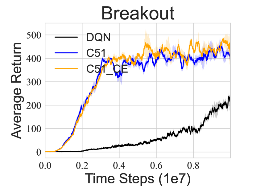
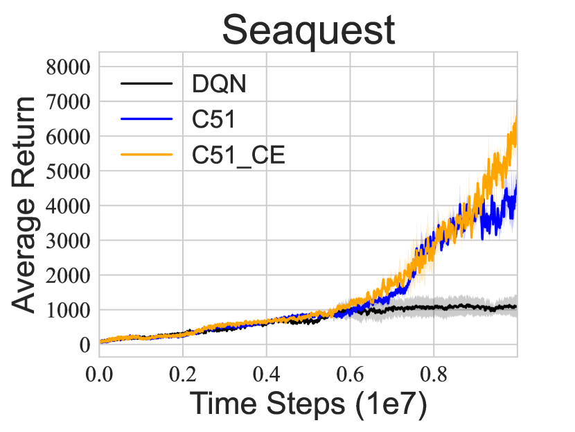
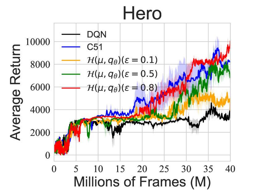
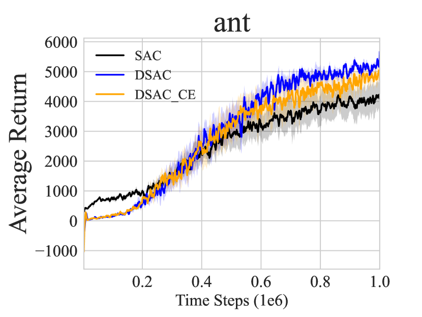
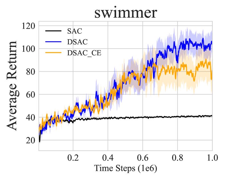
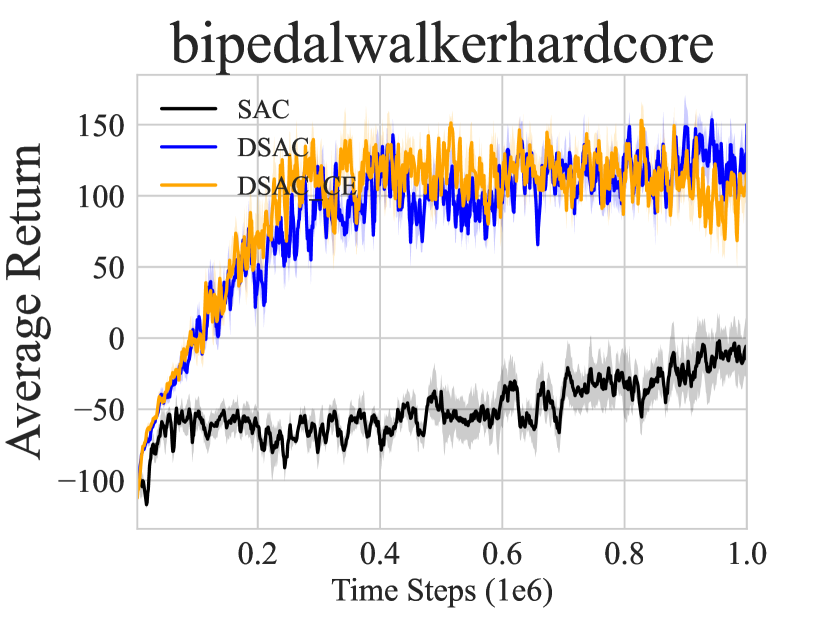
Figure 5: (First row) Learning curves of C51 under cross-entropy loss on Atari games over 3 seeds. (Second row) Learning curves of DSAC with C51 under cross-entropy loss on MuJoCo environments over 5 seeds.

Figure 6 shows that DERAC with different $\lambda$ in Eq. 10 may behave differently in the different environment. Learning curves of DERAC with an increasing $\lambda$ will tend to DSAC (C51), e.g., Bipedalwalkerhardcore, where DERAC with $\lambda=1$ in the green line tends to DSAC (C51) in the blue line. However, DERAC with a small $\lambda$ is likely to outperform DSAC (C51) by only leveraging the expectation effect of return distribution, on Bipedalwalkerhardcore, where DERAC with $\lambda=0,0.5$ bypass DERAC with $\lambda=1.0$.

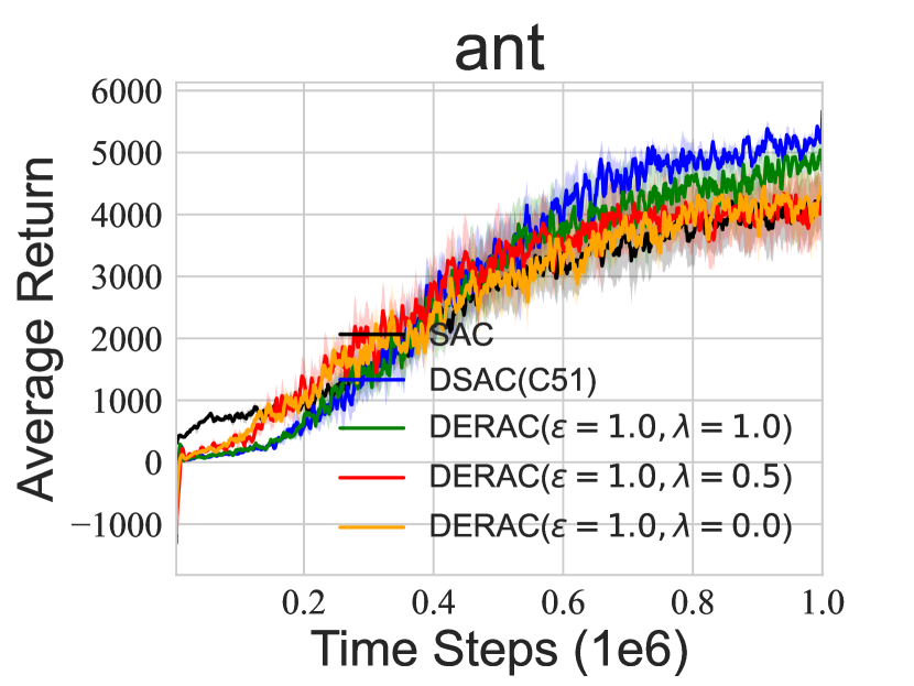
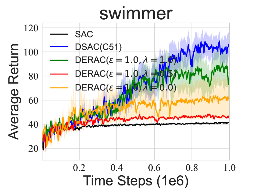
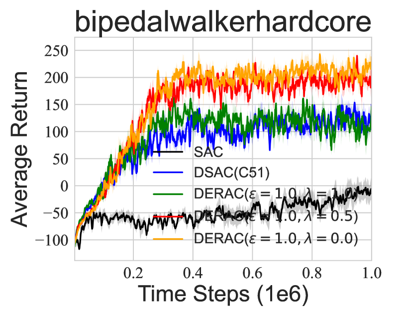
Figure 6: Learning curves of DERAC algorithms across different $\lambda$ on three MuJoCo environments over 5 seeds.

Appendix M Experiments: More Complicated Environments

We further conduct experiments on more complicated environments, including Humanoid (state space as 375, action space as 16) and Walker2D (state space 17, action space 16) to show that DERAC is more likely to outperform on complicated environments. As shown in Figure 7, DERAC (red line) without entropy is competitive to other baselines, including AC (or SAC) and DAC (C51) and especially is superior to DAC (C51) on both complicated environments. In particular, on humanoid, DERAC performs better than both SAC and DAC (C51), and bypasses both AC and DAC (C51) on Walker2D, suggesting its potential on complicated environments.

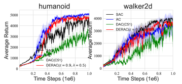
Figure 7: Learning curves of Distributional AC (C51) with the return distribution decomposition on complicated environments, including Humanoid and Walker2D. All results are averaged over 5 seeds. We denote AC as SAC without the leverage of entropy and DAC (C51) as DSAC (C15) without entropy.

Appendix N Environments: Mutual Impacts on DSAC (C51)

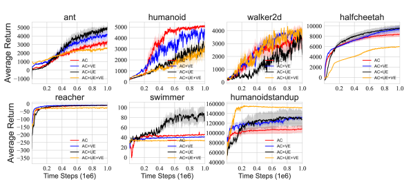
Figure 8: Learning curves of AC, AC+VE (SAC), AC+UE (DAC) and AC+UE+VE (DSAC) over 5 seeds with smooth size 5 across 7 MuJoCo environments where distributional RL part is based on C51.

We presents results on 7 MuJoCo environments and omits Bipedalwalkerhardcore due to some engineering issue when the C51 algorithm interacts with the simulator. Figures 8 showcases that AC+UE (black) tends to perform better than AC (red) except on Humanoid and walker2d. However, when compared with AC+UE, AC+UE+VE (orange) may hurt the performance, e.g. on halfcheetah, ant and swimmer, while further boosts the performance on complicated environments, including humanoidstandup and walker2d. Similar situation is also applicable to AC+VE (blue). All of the conclusions made on DSAC (C51) is similar to DSAC (IQN).

References

- Arjovsky & Bottou (2017) Arjovsky, M. and Bottou, L. Towards principled methods for training generative adversarial networks. International Conference on Learning Representations, 2017, 2017.
- Arjovsky et al. (2017) Arjovsky, M., Chintala, S., and Bottou, L. Wasserstein generative adversarial networks. In International conference on machine learning, pp. 214–223. PMLR, 2017.
- Bellemare et al. (2017a) Bellemare, M. G., Dabney, W., and Munos, R. A distributional perspective on reinforcement learning. International Conference on Machine Learning (ICML), 2017a.
- Bellemare et al. (2017b) Bellemare, M. G., Danihelka, I., Dabney, W., Mohamed, S., Lakshminarayanan, B., Hoyer, S., and Munos, R. The cramer distance as a solution to biased wasserstein gradients. arXiv preprint arXiv:1705.10743, 2017b.
- Bellemare et al. (2022) Bellemare, M. G., Dabney, W., and Rowland, M. Distributional Reinforcement Learning. MIT Press, 2022. http://www.distributional-rl.org.
- Cho et al. (2023) Cho, T., Han, S., Lee, H., Lee, K., and Lee, J. Pitfall of optimism: Distributional reinforcement learning by randomizing risk criterion. Advances in Neural Information Processing Systems, 2023.
- Dabney et al. (2018a) Dabney, W., Ostrovski, G., Silver, D., and Munos, R. Implicit quantile networks for distributional reinforcement learning. International Conference on Machine Learning (ICML), 2018a.
- Dabney et al. (2018b) Dabney, W., Rowland, M., Bellemare, M. G., and Munos, R. Distributional reinforcement learning with quantile regression. Association for the Advancement of Artificial Intelligence (AAAI), 2018b.
- Fan et al. (2020) Fan, J., Wang, Z., Xie, Y., and Yang, Z. A theoretical analysis of deep q-learning. In Learning for Dynamics and Control, pp. 486–489. PMLR, 2020.
- Haarnoja et al. (2017) Haarnoja, T., Tang, H., Abbeel, P., and Levine, S. Reinforcement learning with deep energy-based policies. In International Conference on Machine Learning, pp. 1352–1361. PMLR, 2017.
- Haarnoja et al. (2018) Haarnoja, T., Zhou, A., Abbeel, P., and Levine, S. Soft actor-critic: Off-policy maximum entropy deep reinforcement learning with a stochastic actor. In International conference on machine learning, pp. 1861–1870. PMLR, 2018.
- Han & Sung (2021) Han, S. and Sung, Y. A max-min entropy framework for reinforcement learning. Advances in neural information processing systems (NeurIPS), 2021.
- Hinton et al. (2015) Hinton, G., Vinyals, O., and Dean, J. Distilling the knowledge in a neural network. arXiv preprint arXiv:1503.02531, 2015.
- Huber (2004) Huber, P. J. Robust Statistics, volume 523. John Wiley & Sons, 2004.
- Kuang et al. (2023) Kuang, Q., Zhu, Z., Zhang, L., and Zhou, F. Variance control for distributional reinforcement learning. International Conference on Machine Learning, 2023.
- Lim & Malik (2022) Lim, S. H. and Malik, I. Distributional reinforcement learning for risk-sensitive policies. Advances in Neural Information Processing Systems, 35:30977–30989, 2022.
- Lyle et al. (2019) Lyle, C., Bellemare, M. G., and Castro, P. S. A comparative analysis of expected and distributional reinforcement learning. In Proceedings of the AAAI Conference on Artificial Intelligence, volume 33, pp. 4504–4511, 2019.
- Ma et al. (2020) Ma, X., Xia, L., Zhou, Z., Yang, J., and Zhao, Q. Dsac: Distributional soft actor critic for risk-sensitive reinforcement learning. arXiv preprint arXiv:2004.14547, 2020.
- Ma et al. (2021) Ma, Y. J., Jayaraman, D., and Bastani, O. Conservative offline distributional reinforcement learning. arXiv preprint arXiv:2107.06106, 2021.
- Mavrin et al. (2019) Mavrin, B., Zhang, S., Yao, H., Kong, L., Wu, K., and Yu, Y. Distributional reinforcement learning for efficient exploration. International Conference on Machine Learning (ICML), 2019.
- Mei et al. (2020) Mei, J., Xiao, C., Szepesvari, C., and Schuurmans, D. On the global convergence rates of softmax policy gradient methods. In International Conference on Machine Learning, pp. 6820–6829. PMLR, 2020.
- Mnih et al. (2015) Mnih, V., Kavukcuoglu, K., Silver, D., Rusu, A. A., Veness, J., Bellemare, M. G., Graves, A., Riedmiller, M., Fidjeland, A. K., Ostrovski, G., et al. Human-level control through deep reinforcement learning. nature, 518(7540):529–533, 2015.
- Morimura et al. (2012) Morimura, T., Sugiyama, M., Kashima, H., Hachiya, H., and Tanaka, T. Parametric return density estimation for reinforcement learning. arXiv preprint arXiv:1203.3497, 2012.
- Müller et al. (2019) Müller, R., Kornblith, S., and Hinton, G. When does label smoothing help? arXiv preprint arXiv:1906.02629, 2019.
- Nguyen et al. (2020) Nguyen, T. T., Gupta, S., and Venkatesh, S. Distributional reinforcement learning with maximum mean discrepancy. Association for the Advancement of Artificial Intelligence (AAAI), 2020.
- Riedmiller (2005) Riedmiller, M. Neural fitted q iteration–first experiences with a data efficient neural reinforcement learning method. In European conference on machine learning, pp. 317–328. Springer, 2005.
- Rowland et al. (2018) Rowland, M., Bellemare, M., Dabney, W., Munos, R., and Teh, Y. W. An analysis of categorical distributional reinforcement learning. In International Conference on Artificial Intelligence and Statistics, pp. 29–37. PMLR, 2018.
- Rowland et al. (2019) Rowland, M., Dadashi, R., Kumar, S., Munos, R., Bellemare, M. G., and Dabney, W. Statistics and samples in distributional reinforcement learning. International Conference on Machine Learning (ICML), 2019.
- Rowland et al. (2023a) Rowland, M., Munos, R., Azar, M. G., Tang, Y., Ostrovski, G., Harutyunyan, A., Tuyls, K., Bellemare, M. G., and Dabney, W. An analysis of quantile temporal-difference learning. arXiv preprint arXiv:2301.04462, 2023a.
- Rowland et al. (2023b) Rowland, M., Tang, Y., Lyle, C., Munos, R., Bellemare, M. G., and Dabney, W. The statistical benefits of quantile temporal-difference learning for value estimation. International Conference on Machine Learning, 2023b.
- Shi et al. (2022) Shi, C., Wang, X., Luo, S., Zhu, H., Ye, J., and Song, R. Dynamic causal effects evaluation in a/b testing with a reinforcement learning framework. Journal of the American Statistical Association, pp. 1–13, 2022.
- Sui et al. (2023) Sui, Y., Huang, Y., Zhu, H., and Zhou, F. Adversarial learning of distributional reinforcement learning. In International Conference on Machine Learning, pp. 32783–32796. PMLR, 2023.
- Sun et al. (2022a) Sun, K., Jiang, B., and Kong, L. How does value distribution in distributional reinforcement learning help optimization? arXiv preprint arXiv:2209.14513, 2022a.
- Sun et al. (2022b) Sun, K., Zhao, Y., Liu, Y., Jiang, B., and Kong, L. Distributional reinforcement learning via sinkhorn iterations. arXiv preprint arXiv:2202.00769, 2022b.
- Sun et al. (2023) Sun, K., Liu, Y., Zhao, Y., Yao, H., Jui, S., and Kong, L. Exploring the training robustness of distributional reinforcement learning against noisy state observations. European Conference on Machine Learning and Principles and Practice of Knowledge Discovery in Databases (ECML-PKDD), 2023.
- Sutton & Barto (2018) Sutton, R. S. and Barto, A. G. Reinforcement learning: An Introduction. MIT press, 2018.
- Wasserman (2006) Wasserman, L. All of nonparametric statistics. Springer Science & Business Media, 2006.
- Watkins & Dayan (1992) Watkins, C. J. and Dayan, P. Q-learning. Machine learning, 8(3-4):279–292, 1992.
- Williams & Peng (1991) Williams, R. J. and Peng, J. Function optimization using connectionist reinforcement learning algorithms. Connection Science, 3(3):241–268, 1991.
- Wu et al. (2023) Wu, R., Uehara, M., and Sun, W. Distributional offline policy evaluation with predictive error guarantees. International Conference on Machine Learning, 2023.
- Yang et al. (2019) Yang, D., Zhao, L., Lin, Z., Qin, T., Bian, J., and Liu, T.-Y. Fully parameterized quantile function for distributional reinforcement learning. Advances in neural information processing systems, 32:6193–6202, 2019.
- Zhou et al. (2020) Zhou, F., Wang, J., and Feng, X. Non-crossing quantile regression for distributional reinforcement learning. Advances in Neural Information Processing Systems, 33, 2020.