Transcribe-to-Diarize: Neural Speaker Diarization for Unlimited Number of Speakers using End-to-End Speaker-Attributed ASR

Abstract

This paper presents Transcribe-to-Diarize, a new approach for neural speaker diarization that uses an end-to-end (E2E) speaker-attributed automatic speech recognition (SA-ASR). The E2E SA-ASR is a joint model that was recently proposed for speaker counting, multi-talker speech recognition, and speaker identification from monaural audio that contains overlapping speech. Although the E2E SA-ASR model originally does not estimate any time-related information, we show that the start and end times of each word can be estimated with sufficient accuracy from the internal state of the E2E SA-ASR by adding a small number of learnable parameters. Similar to the target-speaker voice activity detection (TS-VAD)-based diarization method, the E2E SA-ASR model is applied to estimate speech activity of each speaker while it has the advantages of (i) handling unlimited number of speakers, (ii) leveraging linguistic information for speaker diarization, and (iii) simultaneously generating speaker-attributed transcriptions. Experimental results on the LibriCSS and AMI corpora show that the proposed method achieves significantly better diarization error rate than various existing speaker diarization methods when the number of speakers is unknown, and achieves a comparable performance to TS-VAD when the number of speakers is given in advance. The proposed method simultaneously generates speaker-attributed transcription with state-of-the-art accuracy.

Index Terms—  Speaker diarization, rich transcription, speech recognition, speaker counting

1 Introduction

Speaker diarization is a task of recognizing “who spoke when” from audio recordings [1]. A conventional approach is based on speaker embedding extraction for short segmented audio, followed by clustering of the embeddings (sometimes with some constraint regarding the speaker transitions) to attribute the speaker identity to each short segment. Many variants of this approach have been investigated such as the methods using agglomerate hierarchical clustering (AHC) [2], spectral clustering (SC) [3], and variational Bayesian inference [4, 5]. While these approaches showed a good performance for difficult test conditions [6], they cannot handle overlapped speech [7]. Several extensions were also proposed to handle overlapping speech, such as using overlapping detection [8] and speech separation [9]. However, such extensions typically end up with a combination of multiple heuristic rules, which is difficult to optimize.

A neural network-based approach provides more consistent ways to handle the overlapping speech problem by representing the speaker diarization process with a single model. End-to-end neural speaker diarization (EEND) learns a neural network that directly maps an input acoustic feature sequence into a speaker diarization result with permutation-free loss functions [10, 11]. Various extensions of EEND were later proposed to cope with an unknown number of speakers [12, 13]. Region proposal network (RPN)-based speaker diarization [14] uses a neural network that simultaneously performs speech activity detection, speaker embedding extraction, and the resegmentation of detected speech regions. Target-speaker voice activity detection (TS-VAD) [15] is another approach where the neural network is trained to estimate speech activities of all the speakers specified by a set of pre-estimated speaker embeddings. Of these speaker diarization methods, TS-VAD achieved the state-of-the-art (SOTA) results in several diarization tasks [15, 7] including recent international competitions [16, 17]. On the other hand, TS-VAD has a limitation that the number of recognizable speakers is bounded by the number of output nodes of the model.

Speaker diarization performance can also be improved by leveraging the linguistic information. For example, the transcription of the input audio provides a strong clue to estimate the utterance boundaries. Several works were proposed to combine the automatic speech recognition (ASR) with speaker diarization, such as using the word boundary information from ASR [18, 19] or improving the speaker segmentation and clustering based on the information from ASR [20, 21]. While these works showed promising results, the ASR and speaker diarization models were separately trained. Such a combination may not fully utilize the inherent inter-dependency between the speaker diarization and ASR.

With these backgrounds, in this paper, we present Transcribe-to-Diarize, a new speaker diarization approach that uses an end-to-end (E2E) speaker-attributed automatic speech recognition (SA-ASR) [22] as the backbone. The E2E SA-ASR was originally proposed to recognize “who spoke what” by jointly performing speaker counting, multi-talker ASR, and speaker identification from monaural audio that possibly contains overlapping speech. Although the original E2E SA-ASR model does not estimate any information about “when”, in this study, we show that the start and end times of each word can be estimated based on the decoder network of the E2E SA-ASR, making the model to recognize “who spoke when and what”. A rule based method for estimating the time information from the attention weights was investigated in our previous work [23]. Here we substantially improve the diarization accuracy by introducing a learning based framework. In our experiment using the LibriCSS [24] and AMI [25] corpora, we show that the proposed method achieves the SOTA performance in both diarization error rate (DER) and the concatenated minimum-permutation word error rate (cpWER) [26] for the speaker-attributed transcription task.

2 E2E SA-ASR: review

2.1 Overview

The E2E SA-ASR model [22] uses acoustic feature sequence $X\in\mathbb{R}^{f^{a}\times l^{a}}$ and a set of speaker profiles $D=\{d_{k}\in\mathbb{R}^{f^{d}}|k=1,...,K\}$ as input. Here, $f^{a}$ and $l^{a}$ are the feature dimension and length of the feature sequence, respectively. Variable $K$ is the total number of profiles, $d_{k}$ is the speaker embedding (e.g., d-vector [27]) of the $k$-th speaker, and $f^{d}$ is the dimension of the speaker embedding. We assume $D$ includes the profiles of all the speakers present in the observed audio. $K$ can be greater than the actual number of the speakers in the observed audio.

Given $X$ and $D$, the E2E SA-ASR model estimates a multi-talker transcription, i.e., word sequence $Y=(y_{n}\in\{1,...,|\mathcal{V}|\}|n=1,...,N)$ accompanied by the speaker identity of each token $S=(s_{n}\in\{1,...,K\}|n=1,...,N)$. Here, $|\mathcal{V}|$ is the size of the vocabulary $\mathcal{V}$, $y_{n}$ is the word index for the $n$-th token, and $s_{n}$ is the speaker index for the $n$-th token. Following the serialized output training (SOT) framework [28], a multi-talker transcription is represented as a single sequence $Y$ by concatenating the word sequences of the individual speakers with a special “speaker change” symbol $\langle sc\rangle$. For example, the reference token sequence to $Y$ for the three-speaker case is given as $R=\{r^{1}_{1},..,r^{1}_{N^{1}},\langle sc\rangle,r^{2}_{1},..,r^{2}_{N^{2}},\langle sc\rangle,r^{3}_{1},..,r^{3}_{N^{3}},\langle eos\rangle\}$, where $r^{j}_{i}$ represents the $i$-th token of the $j$-th speaker. A special symbol $\langle eos\rangle$ is inserted at the end of all transcriptions to determine the termination of inference. Note that this representation can be used for overlapping speech of any number of speakers.

2.2 Model architecture

The E2E SA-ASR model consists of two attention-based encoder-decoders (AEDs), i.e. an AED for ASR and an AED for speaker identification. The two AEDs depend on each other, and jointly estimate $Y$ and $S$ from $X$ and $D$.

The AED for ASR is represented as,

$$H^{\rm asr} ={\rm AsrEncoder}(X),$$ (1)

$$o_{n} ={\rm AsrDecoder}(y_{[1:n-1]},H^{\rm asr},\bar{d}_{n}).$$ (2)

The AsrEncoder module converts the acoustic feature $X$ into a sequence of hidden embeddings $H^{\rm asr}\in\mathbb{R}^{f^{h}\times l^{h}}$ for ASR (Eq. (1)), where $f^{h}$ and $l^{h}$ are the embedding dimension and the length of the embedding sequence, respectively. The AsrDecoder module then iteratively estimates the output distribution $o_{n}\in\mathbb{R}^{|\mathcal{V}|}$ for $n=1,...,N$ given previous token estimates $y_{[1:n-1]}$, $H^{\rm asr}$, and the weighted speaker profile $\bar{d}_{n}$ (Eq. (2)). Here, $\bar{d}_{n}$ is calculated in the AED for speaker identification, which will be explained later. The posterior probability of token $i$ (i.e. the $i$-th token in $\mathcal{V}$) at the $n$-th decoder step is represented as

$$Pr(y_{n}=i|y_{[1:n-1]},s_{[1:n]},X,D)=o_{n,i},$$ (3)

where $o_{n,i}$ represents the $i$-th element of $o_{n}$.

The AED for speaker identification is represented as

$$H^{spk} ={\rm SpeakerEncoder}(X),$$ (4)

$$q_{n} ={\rm SpeakerDecoder}(y_{[1:n-1]},H^{\rm spk},H^{\rm asr}),$$ (5)

$$\beta_{n,k} =\frac{\exp(\cos(q_{n},d_{k}))}{\sum_{j}^{K}\exp(\cos(q_{n},d_{j}))},$$ (6)

$$\bar{d}_{n} =\sum_{k=1}^{K}\beta_{n,k}d_{k}.$$ (7)

The SpeakerEncoder module converts $X$ into a speaker embedding sequence $H^{\rm spk}\in\mathbb{R}^{f^{h}\times l^{h}}$ that represents the speaker characteristic of $X$ (Eq. (4)). The SpeakerDecoder module then iteratively estimates speaker query $q_{n}\in\mathbb{R}^{f^{d}}$ for $n=1,...,N$ given $y_{[1:n-1]}$, $H^{\rm spk}$ and $H^{\rm asr}$ (Eq. (5)). A cosine similarity-based attention weight $\beta_{n,k}\in\mathbb{R}$ is then calculated for all profiles $d_{k}$ in $D$ given the speaker query $q_{n}$ (Eq. (6)). A posterior probability of person $k$ speaking the $n$-th token is represented by $\beta_{n,k}$ as

$$Pr(s_{n}=k|y_{[1:n-1]},s_{[1:n-1]},X,D)=\beta_{n,k}.$$ (8)

Finally, a weighted average of the speaker profiles is calculated as $\bar{d}_{n}\in\mathbb{R}^{f^{d}}$ (Eq. (7)) to be fed into the AED for ASR (Eq. (2)).

The joint posterior probability $Pr(Y,S|X,D)$ can be represented based on Eqs. (3) and (8) (see [22]). The model parameters are optimized by maximizing $\log Pr(Y,S|X,D)$ over training data.

2.3 E2E SA-ASR based on Transformer

Following [29], a transformer-based network architecture is used for the AsrEncoder, AsrDecoder, and SpeakerDecoder modules. The SpeakerEncoder module is based on Res2Net [30]. Here, we describe only the AsrDecoder because it is necessary to explain the proposed method. Refer to [29] for the details of the other modules.

Our AsrDecoder is almost the same as a conventional transformer-based decoder [31] except for the addition of the weighted speaker profile $\bar{d}_{n}$ at the first layer. The AsrDecoder is represented as

$$z_{[1:n-1],0}^{\rm asr}=\mathrm{PosEnc}(\mathrm{Embed}(y_{[1:n-1]})),$$ (9)

$$\bar{z}^{\rm asr}_{n-1,l}=z^{\rm asr}_{n-1,l-1}$$

$$\hskip 8.53581pt+\mathrm{MHA}_{\rm l}^{\rm asr{\text{-}}self}(z^{\rm asr}_{n-1,l-1},z_{[1:n-1],l-1}^{\rm asr},z_{[1:n-1],l-1}^{\rm asr}),$$ (10)

$$\bar{\bar{z}}^{\rm asr}_{n-1,l}=\bar{z}^{\rm asr}_{n-1,l}+\mathrm{MHA}_{\rm l}^{\rm asr{\text{-}}src}(\bar{z}^{\rm asr}_{n-1,l},H^{\rm asr},H^{\rm asr}),$$ (11)

$$z^{\rm asr}_{n-1,l}=\left\{\begin{array}[]{ll}\bar{\bar{z}}^{\rm asr}_{n-1,l}+\mathrm{FF}_{l}^{\rm asr}(\bar{\bar{z}}^{\rm asr}_{n-1,l}+W^{\rm spk}\cdot\bar{d}_{n})&(l=1)\\ \bar{\bar{z}}^{\rm asr}_{n-1,l}+\mathrm{FF}_{l}^{\rm asr}(\bar{\bar{z}}^{\rm asr}_{n-1,l})&(l>1)\end{array}\right.$$ (14)

$$o_{n}=\mathrm{SoftMax}(W^{o}\cdot z_{n-1,L^{\rm asr}}^{\rm asr}+b^{o}).$$ (15)

Here, $\mathrm{Embed}()$ and $\mathrm{PosEnc}()$ are the embedding function and absolute positional encoding function [31], respectively. $\mathrm{MHA}^{*}_{l}(Q,K,V)$ represents the multi-head attention of the $l$-th layer [31] with query $Q$, key $K$, and value $V$ matrices. $\rm FF_{l}^{\rm asr}()$ is a position-wise feed forward network in the $l$-th layer.

A token sequence $y_{[1:n-1]}$ is first converted into a sequence of embedding $z_{[1:n-1],0}^{\rm asr}\in\mathbb{R}^{f^{h}\times(n-1)}$ (Eq. (9)). For each layer $l$, the self-attention operation (Eq. (10)) and source-target attention operation (Eq. (11)) are applied. Finally, the position-wise feed forward layer is applied to calculate the input to the next layer $z_{n,l+1}^{\rm asr}$ (Eq. (14)). Here, $\bar{d}_{n}$ is added after being multiplied by the weight $W^{spk}\in\mathbb{R}^{f^{h}\times f^{d}}$ in the first layer. Finally, $o_{n}$ is calculated by applying SoftMax function on the final $L^{\rm asr}$-th layer’s output with weight $W^{o}\in\mathbb{R}^{|\mathcal{V}|\times f^{h}}$ and bias $b^{o}\in\mathbb{R}^{|\mathcal{V}|}$ application (Eq. (15)).

Table 1: Comparison of the DER (%) and cpWER (%) on the LibriCSS corpus with the monaural setting. Automatic VAD (i.e. not oracle VAD) was used in all systems. The DER including speaker overlapping regions was evaluated with 0 sec of collar. The number with bold font is the best result with automatic speaker counting, and the number with underline is the best result given oracle number of speakers.

System		Speaker counting		DER for different overlap ratio								cpWER
				0L	0S	10	20	30	40	Avg.
AHC [7]		estimated		16.1	12.0	16.9	23.6	28.3	33.2	22.6		36.7⋆
VBx [7]		estimated		14.6	11.1	14.3	21.5	25.4	31.2	20.5		33.4⋆
SC [7]		estimated		10.9	9.5	13.9	18.9	23.7	27.4	18.3		31.0⋆
RPN [7]		oracle		4.5	9.1	8.3	6.7	11.6	14.2	9.5		27.2⋆
TS-VAD [7]		oracle		6.0	4.6	6.6	7.3	10.3	9.5	7.6		24.4⋆
SC (ours)		estimated		9.0	7.9	11.7	16.5	22.2	25.6	16.4		-
SC (ours)		oracle		7.9	7.7	11.5	16.9	20.9	25.5	16.0		-
Transcribe-to-Diarize		estimated		7.2	9.5	7.2	7.1	10.2	8.9	8.4		12.9
Transcribe-to-Diarize		oracle		6.2	9.5	6.8	7.5	8.6	8.3	7.9		11.6

^⋆ TDNN-F-based hybrid ASR biased by the target-speaker i-vector was applied on top of the diarization results.

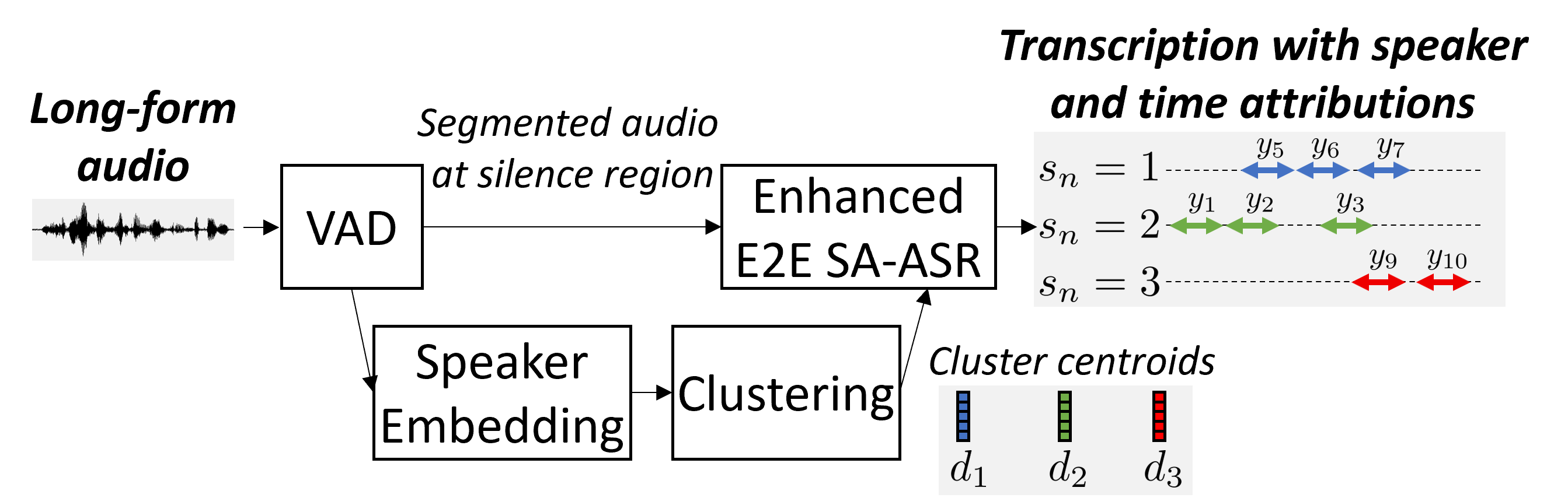
Fig. 1: Overview of the proposed approach.

3 Speaker diarization using E2E SA-ASR

3.1 Procedure overview

The overview of the proposed procedure is shown in Fig. 1. VAD is first applied to the long-form audio to detect silence regions. Then, speaker embeddings are extracted from uniformly segmented audio with a sliding window. A conventional clustering algorithm (in our experiment, spectral clustering) is then applied to obtain the cluster centroids. Finally, the E2E SA-ASR is applied to each VAD-segmented audio with the cluster centroids as the speaker profiles. In this work, the E2E SA-ASR model is extended to generate not only a speaker-attributed transcription but also the start and end times of each token, which can be directly translated to the speaker diarization result. In the evaluation, detected regions for temporarily close tokens (i.e. tokens apart from each other with less than $M$ sec) with the same speaker identities are merged to form a single speaker activity region. We also exclude abnormal estimations where (i) end_time - start_time $\geq$ $N$ sec or (ii) end_time $<$ start_time for a single token. We set $M=2.0$ and $N=2.0$ in our experiment according to the preliminary results.

3.2 Estimating start and end times from Transformer decoder

In this study, we propose to estimate start and end times of $n$-th estimated token from the query $\bar{z}_{n-1,l}^{\rm asr}$ and key $H^{\rm asr}$, which are used in the source-target attention (Eq. (11)), with a small number of learnable parameters. Note that, although there are several prior works that conducted the analysis on the source-target attention, we are not aware of any prior works that directly estimate the start and end times of each token with learnable parameters. It should also be noted that we can not rely on a conventional force-alignment tool (e.g. [32]) because the input audio may be including overlapping speech.

With the proposed method, the probability distribution of start time frame of the $n$-th token over the length of $H^{\rm asr}$ is estimated as

$$\alpha_{n}^{\rm start}=\mathrm{Softmax}(\sum_{l}\frac{(W_{l}^{\rm s,q}\bar{z}_{n-1,l}^{asr})^{\mathsf{T}}(W_{l}^{\rm s,k}H^{\rm asr})}{\sqrt{f^{\rm se}}}).$$ (16)

Here, $f^{\rm se}$ is the dimension of the subspace to estimate the start time frame of each token. The terms $W_{l}^{\rm s,q}\in\mathbb{R}^{f^{\rm se}\times f^{h}}$ and $W_{l}^{\rm s,k}\in\mathbb{R}^{f^{\rm se}\times f^{h}}$ are the affine transforms to map the query and key to the subspace, respectively. The resultant $\alpha_{n}^{\rm start}\in\mathbb{R}^{l^{h}}$ is the scaled dot-product attention accumulated for all layers, and it can be regarded as the probability distribution of the start time frame of $n$-th token over the length of embeddings $H^{\rm asr}$. Similarly, the probability distribution of the end time frame of the $n$-th token, represented by $\alpha_{n}^{\rm end}\in\mathbb{R}^{l^{h}}$, is estimated by replacing $W_{l}^{\rm s,q}$ and $W_{l}^{\rm s,k}$ of Eq (16) with $W_{l}^{\rm e,q}\in\mathbb{R}^{f^{\rm se}\times f^{h}}$ and $W_{l}^{\rm e,k}\in\mathbb{R}^{f^{\rm se}\times f^{h}}$, respectively.

The parameters $W_{l}^{\rm s,q}$, $W_{l}^{\rm s,k}$, $W_{l}^{\rm e,q}$, and $W_{l}^{\rm e,k}$ are learned from training data that includes the reference start and end time indices on the embedding length of $H^{\rm asr}$. In this paper, we apply a cross entropy (CE) objective function on the estimation of $\alpha_{n}^{\rm start}$ and $\alpha_{n}^{\rm end}$ on every token except special tokens $\langle sc\rangle$ and $\langle eos\rangle$. We perform the multi-task training with the objective function of the original E2E SA-ASR model and the objective function of the start-end time estimation with an equal weight to each objective function. In the inference, frames with the maximum value on $\alpha_{n}^{\rm start}$ and $\alpha_{n}^{\rm end}$ are selected as the start and end frames for the $n$-th token, respectively.

Table 2: Comparison of the DER (%) and cpWER (%) on the AMI corpus. The number of speakers was estimated in all systems. The DER including speaker overlapping regions was evaluated with 0 sec of collar based on the reference boundary determined in [5]. SER: speaker error, Miss: miss error, FA: false alarm. DER = SER + Miss + FA.

Audio	System	VAD	dev			eval
			SER / Miss / FA / DER	cpWER		SER / Miss / FA / DER	cpWER
IHM-MIX	AHC [5]	oracle†	6.16 / 13.45 / 0.00 / 19.61	-		6.87 / 14.56 / 0.00 / 21.43	-
IHM-MIX	VBx [5]	oracle†	2.88 / 13.45 / 0.00 / 16.33	-		4.43 / 14.56 / 0.00 / 18.99	-
IHM-MIX	SC	automatic	3.37 / 14.89 / 9.67 / 27.93	23.1‡		3.45 / 16.34 / 9.53 / 29.32	23.4‡
IHM-MIX	Transcribe-to-Diarize	automatic	3.05 / 11.46 / 9.00 / 23.51	15.9		2.47 / 14.24 / 7.72 / 24.43	16.4
IHM-MIX	Transcribe-to-Diarize	oracle†	2.83 /   9.69 / 3.46 / 15.98	16.3		1.78 / 11.71 / 3.10 / 16.58	15.1
SDM	SC	automatic	3.50 / 21.93 / 4.54 / 29.97	28.6‡		3.69 / 24.84 / 4.14 / 32.68	30.3‡
SDM	Transcribe-to-Diarize	automatic	3.48 / 15.93 / 7.17 / 26.58	22.6		2.86 / 19.20 / 6.07 / 28.12	24.9
SDM	Transcribe-to-Diarize	oracle†	3.38 / 10.62 / 3.28 / 17.27	21.5		2.69 / 12.82 / 3.04 / 18.54	22.2

^† Reference boundary information was used to segment the audio at each silence region.
        ^‡ Single-talker Conformer-based ASR pre-trained by 75K-data and fine-tuned by AMI [33] was used on top of the speaker diarization result.

4 Evaluation Results

We evaluated the proposed method with the LibriCSS corpus [24] and the AMI meeting corpus [25]. We used DER as the primary performance metric. We also used the cpWER [26] for the evaluation of speaker-attributed transcription.

4.1 Evaluation on the LibriCSS corpus

4.1.1 Experimental settings

The LibriCSS corpus [24] is a set of 8-speaker recordings made by playing back “test_clean” of LibriSpeech in a real meeting room. The recordings are 10 hours long in total, and they are categorized by the speaker overlap ratio from 0% to 40%. We used the first channel of the 7-ch microphone array recordings in this experiment.

We used the model architecture described in [33]. The AsrEncoder consisted of 2 convolution layers that subsamples the time frames by a factor of 4, followed by 18 Conformer [34] layers. The AsrDecoder consisted of 6 layers and 16k subwords were used as a recognition unit. The SpeakerEncoder was based on Res2Net [30] and designed to be the same with that of the speaker profile extractor. Finally, SpeakerDecoder consisted of 2 transformer layers. We used a 80-dim log mel filterbank extracted every 10 msec as the input feature, and the Res2Net-based d-vector extractor [9] trained by VoxCeleb corpora [35, 36] was used to extract a 128-dim speaker embedding. We set $f^{\rm se}=64$ for the start and end-time estimation. See [33] for more details of the model architecture.

We used a similar multi-speaker training data set to the one used in [23] except that we newly introduced a small amount of training samples with no overlap between the speaker activities. The training data were generated by mixing 1 to 5 utterances of 1 to 5 speakers from LibriSpeech with random delays being applied to each utterance, where 90% of the delay was designed to have speaker overlaps while 10% of the delay was designed to have no speaker overlaps with 0 to 1 sec of intermediate silence. Randomly generated room impulse responses and noise were also added to simulate the reverberant recordings. We used the word alignment information on the original LibriSpeech utterances (i.e. the ones before mixing) generated with the Montreal Forced Aligner [32]. If one word consists of multiple subwords, we divided the duration of such a word by the number of subwords to determine the start and end times of each subword. We initialized the ASR block by the model trained with SpecAugment as described in [29], and performed 160k iterations of training based only with $\log Pr(Y,S|X,D)$ with a mini-batch of 6,000 frames with 8 GPUs. Noam learning rate schedule with peak learning rate of 0.0001 after 10k iterations was used. We then reset the learning rate schedule, and performed further 80k iterations of training with the training objective function that includes the CE objective function for the start and end times of each token.

In the evaluation, we first applied the WebRTC VAD with the least aggressive setting, and extracted the d-vector from speech region based on the 1.5 sec of sliding window with 0.75 sec of window shift. Then, we applied the speaker counting and clustering based on the normalized maximum eigengap-based spectral clustering (NME-SC) [3]. Then, we cut the audio into a short segment at the middle of silence region detected by WebRTC VAD. We split the audio when the duration of the audio was longer than the 20 sec. We then ran the E2E SA-ASR for each segmented audio with the average speaker embeddings from the speaker cluster generated by the NME-SC.

4.1.2 Evaluation Results

Table 1 shows the result on the LibriCSS corpus with various diarization methods. With the estimated number of speakers, our proposed method achieved a significantly better average DER (8.4%) than any other speaker diarization techniques (16.0% to 22.6%). We also confirmed that the proposed method achieved the DER of 7.9% when the number of speakers was known, which was close to the strong result by TS-VAD (7.6%) that was specifically trained for the 8-speaker condition. We observed that the proposed method was especially good for the inputs with high overlap ratio, such as 30% to 40%. It should be also noted that the cpWER by the proposed method (11.6% with the oracle number of speakers and 12.9% with the estimated number of speakers) were significantly better than the prior works, and they are the SOTA results for the monaural setting of LibriCSS with no prior knowledge on speakers.

4.2 Evaluation on the AMI corpus

4.2.1 Experimental settings

We also evaluated the proposed method with the AMI meeting corpus [25], which is a set of real meeting recordings of four participants. For the evaluation, we used single distant microphone (SDM) recordings or the mixture of independent headset microphones, called IHM-MIX. We used scripts of the Kaldi toolkit [37] to partition the recordings into training, development, and evaluation sets. The total durations of the three sets were 80.2 hours, 9.7 hours, and 9.1 hours, respectively.

We initialized the model with a well-trained E2E SA-ASR model based on the 75 thousand hours of ASR training data, VoxCeleb corpus, and AMI-training data, the detail of which is described in [33]. We performed 2,500 training iterations by using the AMI training corpus with a mini-batch of 6,000 frames with 8 GPUs and a linear decay learning rate schedule with peak learning rate of 0.0001. We used the word boundary information obtained from the reference annotations of the AMI corpus. Unlike the experiment on the LibriCSS, we updated only $W_{l}^{\rm s,q}$, $W_{l}^{\rm s,k}$, $W_{l}^{\rm e,q}$, and $W_{l}^{\rm e,k}$ by freezing other pre-trained parameters because overfitting was observed otherwise in our preliminary experiment.

4.2.2 Evaluation Results

The evaluation results are shown in Table 2. The proposed method achieved significantly better DERs for both SDM and IHM-MIX conditions. Especially, we observed significant improvements in the miss error rate, which indicates the effectiveness of the proposed method in the speaker overlapping regions. The proposed model, pre-trained on a large-scale data [38, 33], simultaneously achieved the SOTA cpWER on the AMI dataset among fully automated monaural SA-ASR systems.

5 Conclusion

This paper presented the new approach for speaker diarization using the E2E SA-ASR model. In the experiment with the LibriCSS corpus and the AMI meeting corpus, the proposed method achieved significantly better DER over various speaker diarization methods under the condition of the speaker number being unknown while achieving almost the same DER as TS-VAD when the oracle speaker number is available.

References

- [1] T. J. Park et al., “A review of speaker diarization: Recent advances with deep learning,” arXiv:2101.09624, 2021.
- [2] D. Garcia-Romero et al., “Speaker diarization using deep neural network embeddings,” in ICASSP, 2017, pp. 4930–4934.
- [3] T. J. Park, K. J. Han, M. Kumar, and S. Narayanan, “Auto-tuning spectral clustering for speaker diarization using normalized maximum eigengap,” IEEE Signal Processing Letters, vol. 27, pp. 381–385, 2019.
- [4] M. Diez, L. Burget, and P. Matejka, “Speaker diarization based on bayesian hmm with eigenvoice priors.” in Odyssey, 2018, pp. 147–154.
- [5] F. Landini, J. Profant, M. Diez, and L. Burget, “Bayesian HMM clustering of x-vector sequences (VBx) in speaker diarization: theory, implementation and analysis on standard tasks,” Computer Speech & Language, vol. 71, p. 101254, 2022.
- [6] N. Ryant et al., “The second DIHARD diarization challenge: Dataset, task, and baselines,” Interspeech, pp. 978–982, 2019.
- [7] D. Raj et al., “Integration of speech separation, diarization, and recognition for multi-speaker meetings: System description, comparison, and analysis,” in SLT, 2021, pp. 897–904.
- [8] L. Bullock, H. Bredin, and L. P. Garcia-Perera, “Overlap-aware diarization: Resegmentation using neural end-to-end overlapped speech detection,” in ICASSP, 2020, pp. 7114–7118.
- [9] X. Xiao et al., “Microsoft speaker diarization system for the VoxCeleb speaker recognition challenge 2020,” in ICASSP, 2021, pp. 5824–5828.
- [10] Y. Fujita, N. Kanda, S. Horiguchi, K. Nagamatsu, and S. Watanabe, “End-to-end neural speaker diarization with permutation-free objectives,” Interspeech, pp. 4300–4304, 2019.
- [11] Y. Fujita, N. Kanda, S. Horiguchi, Y. Xue, K. Nagamatsu, and S. Watanabe, “End-to-end neural speaker diarization with self-attention,” in ASRU, 2019, pp. 296–303.
- [12] S. Horiguchi, Y. Fujita, S. Watanabe, Y. Xue, and K. Nagamatsu, “End-to-end speaker diarization for an unknown number of speakers with encoder-decoder based attractors,” in Interspeech, 2020, pp. 269–273.
- [13] K. Kinoshita, M. Delcroix, and N. Tawara, “Integrating end-to-end neural and clustering-based diarization: Getting the best of both worlds,” in ICASSP, 2021, pp. 7198–7202.
- [14] Z. Huang et al., “Speaker diarization with region proposal network,” in ICASSP, 2020, pp. 6514–6518.
- [15] I. Medennikov et al., “Target-speaker voice activity detection: A novel approach for multi-speaker diarization in a dinner party scenario,” in Interspeech, 2020, pp. 274–278.
- [16] N. Ryant et al., “The third DIHARD diarization challenge,” arXiv:2012.01477, 2020.
- [17] W. Wang et al., “The DKU-DukeECE-Lenovo system for the diarization task of the 2021 VoxCeleb speaker recognition challenge,” arXiv:2109.02002, 2021.
- [18] J. Huang, E. Marcheret, K. Visweswariah, and G. Potamianos, “The IBM RT07 evaluation systems for speaker diarization on lecture meetings,” in Multimodal Technologies for Perception of Humans. Springer, 2007, pp. 497–508.
- [19] J. Silovsky, J. Zdansky, J. Nouza, P. Cerva, and J. Prazak, “Incorporation of the ASR output in speaker segmentation and clustering within the task of speaker diarization of broadcast streams,” in MMSP, 2012, pp. 118–123.
- [20] T. J. Park et al., “Speaker diarization with lexical information,” in Interspeech, 2019, pp. 391–395.
- [21] W. Xia et al., “Turn-to-diarize: Online speaker diarization constrained by transformer transducer speaker turn detection,” arXiv:2109.11641, 2021.
- [22] N. Kanda et al., “Joint speaker counting, speech recognition, and speaker identification for overlapped speech of any number of speakers,” in Interspeech, 2020, pp. 36–40.
- [23] ——, “Investigation of end-to-end speaker-attributed ASR for continuous multi-talker recordings,” in SLT, 2021, pp. 809–816.
- [24] Z. Chen, T. Yoshioka, L. Lu, T. Zhou, Z. Meng, Y. Luo, J. Wu, and J. Li, “Continuous speech separation: dataset and analysis,” in ICASSP, 2020, pp. 7284–7288.
- [25] J. Carletta et al., “The AMI meeting corpus: A pre-announcement,” in International workshop on machine learning for multimodal interaction, 2005, pp. 28–39.
- [26] S. Watanabe et al., “CHiME-6 challenge: Tackling multispeaker speech recognition for unsegmented recordings,” in CHiME 2020, 2020.
- [27] E. Variani, X. Lei, E. McDermott, I. L. Moreno, and J. Gonzalez-Dominguez, “Deep neural networks for small footprint text-dependent speaker verification,” in ICASSP, 2014, pp. 4052–4056.
- [28] N. Kanda, Y. Gaur, X. Wang, Z. Meng, and T. Yoshioka, “Serialized output training for end-to-end overlapped speech recognition,” in Interspeech, 2020, pp. 2797–2801.
- [29] N. Kanda et al., “End-to-end speaker-attributed ASR with Transformer,” in Interspeech, 2021, pp. 4413–4417.
- [30] S. Gao, M.-M. Cheng, K. Zhao, X.-Y. Zhang, M.-H. Yang, and P. H. Torr, “Res2net: A new multi-scale backbone architecture,” IEEE trans. on PAMI, 2019.
- [31] A. Vaswani et al., “Attention is all you need,” in NIPS, 2017, pp. 6000–6010.
- [32] M. McAuliffe, M. Socolof, S. Mihuc, M. Wagner, and M. Sonderegger, “Montreal forced aligner: Trainable text-speech alignment using Kaldi,” in Interspeech, 2017, pp. 498–502.
- [33] N. Kanda et al., “A comparative study of modular and joint approaches for speaker-attributed asr on monaural long-form audio,” in ASRU, 2021.
- [34] A. Gulati et al., “Conformer: Convolution-augmented Transformer for speech recognition,” Interspeech, pp. 5036–5040, 2020.
- [35] A. Nagrani, J. S. Chung, and A. Zisserman, “VoxCeleb: A large-scale speaker identification dataset,” in Interspeech, 2017, pp. 2616–2620.
- [36] J. S. Chung, A. Nagrani, and A. Zisserman, “VoxCeleb2: Deep speaker recognition,” in Interspeech, 2018, pp. 1086–1090.
- [37] D. Povey et al., “The Kaldi speech recognition toolkit,” in ASRU, 2011.
- [38] N. Kanda et al., “Large-scale pre-training of end-to-end multi-talker ASR for meeting transcription with single distant microphone,” in Interspeech, 2021, pp. 3430–3434.