The Gromov-Hausdorff distance between ultrametric spaces:
its structure and computation

Abstract

The Gromov-Hausdorff distance ($d_{\mathrm{GH}}$) provides a natural way of quantifying the dissimilarity between two given metric spaces. It is known that computing $d_{\mathrm{GH}}$ between two finite metric spaces is NP-hard, even in the case of finite ultrametric spaces which are highly structured metric spaces in the sense that they satisfy the so-called strong triangle inequality. Ultrametric spaces naturally arise in many applications such as hierarchical clustering, phylogenetics, genomics, and even linguistics. By exploiting the special structures of ultrametric spaces, (1) we identify a one parameter family $\{d_{\mathrm{GH}}^{\scriptscriptstyle{(p)}}\}_{p\in[1,\infty]}$ of distances defined in a flavor similar to the Gromov-Hausdorff distance on the collection of finite ultrametric spaces, and in particular $d_{\mathrm{GH}}^{\scriptscriptstyle{(1)}}=d_{\mathrm{GH}}$. The extreme case when $p=\infty$, which we also denote by $u_{\mathrm{GH}}$, turns out to be an ultrametric on the collection of ultrametric spaces. Whereas for all $p\in[1,\infty)$, $d_{\mathrm{GH}}^{\scriptscriptstyle{(p)}}$ yields NP-hard problems, we prove that surprisingly $u_{\mathrm{GH}}$ can be computed in polynomial time. The proof is based on a structural theorem for $u_{\mathrm{GH}}$ established in this paper; (2) inspired by the structural theorem for $u_{\mathrm{GH}}$, and by carefully leveraging properties of ultrametric spaces, we also establish a structural theorem for $d_{\mathrm{GH}}$ when restricted to ultrametric spaces. This structural theorem allows us to identify special families of ultrametric spaces on which $d_{\mathrm{GH}}$ is computationally tractable. These families are determined by properties related to the doubling constant of metric space. Based on these families, we devise a fixed-parameter tractable (FPT) algorithm for computing the exact value of $d_{\mathrm{GH}}$ between ultrametric spaces. We believe ours is the first such algorithm to be identified.

1 Introduction and main results

Edwards [14] and Gromov [17] independently introduced a notion nowadays called the Gromov-Hausdorff distance $d_{\mathrm{GH}}$ for comparing metric spaces. This distance enjoys many pleasing mathematical properties: if we let $\mathcal{M}$ denote the collection of all compact metric spaces, then modulo isometry, $(\mathcal{M},d_{\mathrm{GH}})$ is a complete and separable metric space [35, Proposition 43], with rich pre-compact classes [18]. It has also recently been proved that this space is geodesic [20, 9]. This distance has been widely used in differential geometry [35], as a model for shape matching procedures [29, 5], and applied algebraic topology [8] for establishing stability properties of invariants.

Despite admitting many lower bounds which can be computed in polynomial time [8, 30], computing $d_{\mathrm{GH}}$ itself between arbitrary finite metric spaces leads to solving certain generalized quadratic assignment problems [30] which have been shown to be NP-hard [39, 40, 2]. In fact, in [40] Schmiedl proved the following stronger result (see however [28] for the case of point sets on the real line where the authors describe a poly time approximation algorithm):

Theorem 1 ([40, Corollary 3.8]).

The Gromov-Hausdorff distance cannot be approximated within any factor less than 3 in polynomial time, unless $\mathcal{P}=\mathcal{NP}$.

The proof of this result reveals that the claim still holds even in the case of ultrametric spaces. An ultrametric space $(X,d_{X})$ is a metric space which satisfies the strong triangle inequality:

$$\forall x,x^{\prime},x^{\prime\prime}\in X,\text{ one has }d_{X}(x,x^{\prime})\leq\max\left(d_{X}(x,x^{\prime\prime}),d_{X}(x^{\prime\prime},x^{\prime})\right).$$

In this paper, we will henceforth use $u_{X}$ instead of $d_{X}$ to represent an ultrametric. Ultrametric spaces appear in many applications: they arise in statistics as a geometric encoding of dendrograms [21, 7], in taxonomy and phylogenetics [41] as representations of phylogenies, and in linguistics [38]. In theoretical computer science, ultrametric spaces arise as building blocks for the probabilistic approximation of finite metric spaces [4].

In many of the aforementioned applications (including phylogenetics), in order to characterize the difference between relevant objects, it is important to compare ultrametric spaces via meaningful metrics. This is one of the main motivations behind our study of the Gromov-Hausdorff distance between ultrametric spaces.

Being a well understood and highly structured type of metric spaces, we are particularly interested in exploiting possible advantages associated to either restricting or adapting $d_{\mathrm{GH}}$ to the collection $\mathcal{U}^{\mathrm{fin}}$ of all finite ultrametric spaces. In this paper, we provide positive answers to the following two questions naturally arising from trying to bypass/overcome the hardness result in Theorem 1:

1. Is there any suitable variant of the Gromov-Hausdorff distance on the collection of finite ultrametric spaces which can be approximated/computed in polynomial time?

3. Is there any subcollection of ultrametric spaces on which the Gromov-Hausdorff distance can be approximated/computed in polynomial time?

In this paper we provide positive answers to these two questions and in the course of answering these questions, we establish structural theorems for both $d_{\mathrm{GH}}$ and a suitable ultrametric variant $u_{\mathrm{GH}}$ which in each case allow us to convert the problem of comparing two given spaces into instances of the problem on strictly smaller spaces.

Related work

The Gromov-Hausdorff ultrametric, which we denote by $u_{\mathrm{GH}}$, on the collection $\mathcal{U}$ of compact ultrametric spaces was first introduced by Zarichnyi [43] in 2005 as an ultrametric counterpart to $d_{\mathrm{GH}}$. Moreover, the author proved that $(\mathcal{U},u_{\mathrm{GH}})$ is a complete but not separable (ultra) metric space, where $\mathcal{U}$ denotes the collection of all compact ultrametric spaces. $u_{\mathrm{GH}}$ was further studied by Qiu in [37] where the author established several characterizations of $u_{\mathrm{GH}}$ similar to the classical ones for $d_{\mathrm{GH}}$ (cf. [6, Chapter 7]) such as those arising via the notions of $\varepsilon$-isometry and $(\varepsilon,\delta)$-approximation. Qiu has also found a suitable version of Gromov’s pre-compactness theorem for $(\mathcal{U},u_{\mathrm{GH}})$.

Phylogenetic tree shapes (unlabled rooted trees) are closely related to ultrametric spaces. In [11], Colijn and Plazzotta studied a metric between tree shapes to compare evolutionary trees of influenza. In [27], Liebscher studied a class of metrics analogous to $d_{\mathrm{GH}}$ between unrooted phylogenetic trees. In [26], Lafond et al. extended different types of metrics on phylogenetic trees to metrics between tree shapes via optimization over permutations of labels. They studied the computational aspect of these metric extensions. In particular, they proved that computing the extension of the path distance is NP-complete via a similar argument used for proving that approximating $d_{\mathrm{GH}}$ between merge trees in NP-complete [2]. Moreover, they devised an FPT algorithm which computes the extension of the so-called Robinson-Foulds distances. Their FPT algorithm is a recursive algorithm comparing subtrees of nodes at each iteration, which is of similar flavor to our algorithms (Algorithms 2 and 4) for computing $d_{\mathrm{GH}}$ between ultrametric spaces.

In [15], Touli and Wang devised FPT algorithms for the computation of the interleaving distance $d_{\mathrm{I}}$ between merge trees [32]. Since any finite ultrametric space can be naturally represented by a merge tree (see for example [16]) it turns out that $d_{\mathrm{I}}$ between ultrametric spaces as merge trees is a 2-approximation of $d_{\mathrm{GH}}$ between the ultrametric spaces (see [31, Corollary 6.13]). Thus, one could potentially adapt the algorithm from [15] for computing a 2-approximation for $d_{\mathrm{GH}}$ between ultrametric spaces, which is FPT. In this paper we obtain essentially the same time complexity for the exact computation of $d_{\mathrm{GH}}$ (see Remark 46) via algorithms specifically tailored for ultrametric spaces.

1.1 Our results

In this section, we summarize our main results obtained in the course of answering the two major questions mentioned above.

1.1.1 Polynomial time computable variant of $d_{\mathrm{GH}}$

Let $(X,d_{X})$ and $(Y,d_{Y})$ be two metric spaces. A correspondence $R$ between the underlying sets $X$ and $Y$ is any subset of $X\times Y$ such that the images of $R$ under the canonical projections $p_{X}:X\times Y\rightarrow X$ and $p_{Y}:X\times Y\rightarrow Y$ are full: $p_{X}(R)=X$ and $p_{Y}(R)=Y$. Then, the Gromov-Hausdorff distance $d_{\mathrm{GH}}$ between $X$ and $Y$ is defined as follows [29]:

$$d_{\mathrm{GH}}(X,Y)\coloneqq\frac{1}{2}\inf_{R}\sup_{(x,y),(x^{\prime},y^{\prime})\in R}|d_{X}(x,x^{\prime})-d_{Y}(y,y^{\prime})|,$$ (1)

where the infimum is taken over all correspondences $R$ between $X$ and $Y$. The term appeared above $\sup_{(x,y),(x^{\prime},y^{\prime})\in R}|d_{X}(x,x^{\prime})-d_{Y}(y,y^{\prime})|$ is called the distortion of $R$, denoted by $\mathrm{dis}(R)$.

We modify Equation (1) to obtain a one-parameter family of related quantities: given $p\in[1,\infty)$, define a quantity $d_{\mathrm{GH}}^{\scriptscriptstyle{(p)}}(X,Y)$ as follows:

$$d_{\mathrm{GH}}^{\scriptscriptstyle{(p)}}(X,Y)\coloneqq 2^{-\frac{1}{p}}\inf_{R}\sup_{(x,y),(x^{\prime},y^{\prime})\in R}\left|(d_{X}(x,x^{\prime}))^{p}-(d_{Y}(y,y^{\prime}))^{p}\right|^{\frac{1}{p}}.$$ (2)

In this way, as $p$ increases, the discrepancy between large distance values is more heavily penalized. It turns out that for each $p\in[1,\infty)$, $d_{\mathrm{GH}}^{\scriptscriptstyle{(p)}}$ is a metric on the collection $\mathcal{U}$ of all compact ultrametric spaces. Moreover, we will later show as a consequence of Theorem 1 the following as one of our motivations of considering $d_{\mathrm{GH}}^{\scriptscriptstyle{(p)}}$:

Corollary 2.

For each $p\in[1,\infty)$ and for any $X,Y\in\mathcal{U}^{\mathrm{fin}}$, $d_{\mathrm{GH}}^{\scriptscriptstyle{(p)}}(X,Y)$ cannot be approximated within any factor less than $3^{\frac{1}{p}}$ in polynomial time, unless $\mathcal{P}=\mathcal{NP}$.

Note that the factor $3^{\frac{1}{p}}$ approaches $1$ as $p\rightarrow\infty$. This suggests us considering $d_{\mathrm{GH}}^{\scriptscriptstyle{(\infty)}}\coloneqq\lim_{p\rightarrow\infty}d_{\mathrm{GH}}^{\scriptscriptstyle{(p)}}$, which could potentially be a computationally tractable quantity. Before stating our computational result for $d_{\mathrm{GH}}^{\scriptscriptstyle{(\infty)}}$, it is worth mentioning that $d_{\mathrm{GH}}^{\scriptscriptstyle{(\infty)}}$ turns out to be an ultrametric on $\mathcal{U}$. Moreover, it actually coincides with the Gromov-Hausdorff ultrametric $u_{\mathrm{GH}}$ defined by Zarichnyi [43]. In the sequel, we will hence use $u_{\mathrm{GH}}$ to denote $d_{\mathrm{GH}}^{\scriptscriptstyle{(\infty)}}$.

One of our main contributions in the paper is the following structural characterization of $u_{\mathrm{GH}}$. This structural result eventually leads to a polynomial time computable algorithm for computing $u_{\mathrm{GH}}$ which we will state later.

Theorem 3 (Structural theorem for $u_{\mathrm{GH}}$).

For any $X,Y\in\mathcal{U}^{\mathrm{fin}}$ one has that

$$u_{\mathrm{GH}}(X,Y)=\min\left\{t\geq 0:\,\left(X_{\mathfrak{c}(t)},u_{X_{\mathfrak{c}(t)}}\right)\,\mbox{is isometric to}\,\left(Y_{\mathfrak{c}(t)},u_{Y_{\mathfrak{c}(t)}}\right)\right\}.$$

Here $\left(X_{\mathfrak{c}(t)},u_{X_{\mathfrak{c}(t)}}\right)$ is the $t$-closed quotient of $X$ where $x$ and $x^{\prime}$ are identified if $u_{X}(x,x^{\prime})\leq t$ (cf. Definition 9). See Figure 1 for an illustration of Theorem 3.

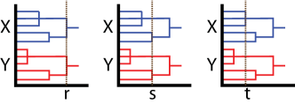
Figure 1: Illustration of Theorem 3. We represent two ultrametric spaces $X$ and $Y$ as dendrograms (See Theorem 14 for more details.). Imagine that we move a vertical dotted line from right to left ($r>s>t$) to obtain successive quotient spaces according to the parameter indicated by the line, as described in Definition 9. It is obvious from the figure that ($\cong$ denotes isometry) $X_{\mathfrak{c}(r)}\cong Y_{\mathfrak{c}(r)}$, $X_{\mathfrak{c}(s)}\cong Y_{\mathfrak{c}(s)}$, $X_{\mathfrak{c}(t)}\cong Y_{\mathfrak{c}(t)}$, and that $t$ is the minimum value such that the resulting quotient spaces are isometric. Thus, $u_{\mathrm{GH}}(X,Y)=t.$

Based on Theorem 3, we devise an algorithm for computing $u_{\mathrm{GH}}$ as follows. For a finite ultrametric space $X$, the isometry type of $X_{\mathfrak{c}(t)}$ only changes finitely many times along $0\leq t<\infty$. In fact, the set of all $t$s when $X_{\mathfrak{c}(t)}$ changes its isometry type is exactly the spectrum $\mathrm{spec}(X)\coloneqq\{u_{X}(x,x^{\prime}):\,x,x^{\prime}\in X\}$ of $X$. Then, in order to compute $u_{\mathrm{GH}}(X,Y)$, we simply check whether $X_{\mathfrak{c}(t)}\cong Y_{\mathfrak{c}(t)}$, starting from the largest $t$ and progressively scanning all possible $t$s until reaching the smallest $t$ in $\mathrm{spec}(X)\bigcup\mathrm{spec}(Y)$; the smallest $t$ such that $X_{\mathfrak{c}(t)}\cong Y_{\mathfrak{c}(t)}$ will be $u_{\mathrm{GH}}(X,Y)$. Since ultrametric spaces can be regarded as weighted trees (cf. Section A.1), determining whether two ultrametric spaces are isometric is equivalent to determining whether two weighted trees are isomorphic, which can be achieved in polynomial time on the number of vertices involved.

We prove that computing $u_{\mathrm{GH}}$ can be done in time $O(n\log(n))$ where $n$ is the maximum of the cardinalities of $X$ and $Y$ (cf. Theorem 29 and Remark 30). See Section 4 for the pseudocode (cf. Algorithm 1) of the algorithm described above and a detailed complexity analysis, and also see Appendix B for an extension of $u_{\mathrm{GH}}$ to the case of ultra-dissimilarity spaces. We also remark that our computational results regarding the determination of $u_{\mathrm{GH}}$ (between finite ultrametric spaces) can be interpreted as providing a novel computationally tractable instance of the well known quadratic assignment problem (cf. Remark 31).

In the end, we summarize our complexity results in Figure 2

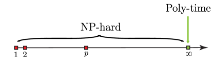
Figure 2: Complexity of $d_{\mathrm{GH}}^{\scriptscriptstyle{(p)}}$. Computing/approximating $d_{\mathrm{GH}}^{\scriptscriptstyle{(p)}}$ is NP-hard for each $p\in[1,\infty)$ whereas computing $d_{\mathrm{GH}}^{\scriptscriptstyle{(\infty)}}$ can be done in polynomial time.

1.1.2 Polynomial time computable family with respect to $d_{\mathrm{GH}}$

Inspired by the usefulness of Theorem 3 for $u_{\mathrm{GH}}$, we exploit special properties of ultrametric spaces and establish a structural theorem for $d_{\mathrm{GH}}$ between ultrametric spaces (Theorem 4).

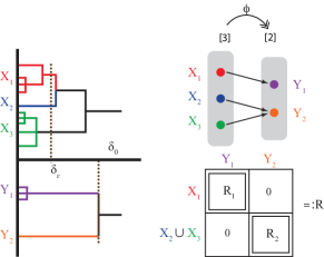
Figure 3: Illustration of the claim in Theorem 4.

Below, $X_{\mathfrak{o}(t)}$ denotes the $t$-open partition of $X$ where $x$ and $x^{\prime}$ belong to the same block if $u_{X}(x,x^{\prime})<t$ (cf. Definition 11) and we call any correspondence $R$ between $X$ and $Y$ with distortion (cf. Section 3) bounded above by $\varepsilon\geq 0$ an $\varepsilon$-correspondence. Given a metric space $X$ and $\varepsilon\geq 0$, we let $\delta_{\varepsilon}(X)\coloneqq\mathrm{diam}(X)-\varepsilon$. With this notation, $\delta_{0}(X)=\mathrm{diam}(X)$.

Theorem 4 (Structural theorem for $d_{\mathrm{GH}}$).

Let $X,Y\in\mathcal{U}^{\mathrm{fin}}$ and $\varepsilon\geq 0$ be such that

$$|\delta_{0}(X)-\delta_{0}(Y)|\leq\varepsilon<\delta_{0}(Y).$$ (3)

Consider the following open partitions

$$X_{\mathfrak{o}\left(\delta_{\varepsilon}(Y)\right)}:=\left\{X_{i}\right\}_{i=1}^{N_{X}}\,\,\,\mbox{and}\,\,\,\,Y_{\mathfrak{o}\left(\delta_{0}(Y)\right)}:=\left\{Y_{j}\right\}_{j=1}^{N_{Y}}.$$

Then, there exists an $\varepsilon$-correspondence between $X$ and $Y$ if and only if:

• there exists a surjection $\Psi:[N_{X}]\twoheadrightarrow[N_{Y}]$ and, with this surjection,

• for every $j\in[N_{Y}]$ there exists an $\varepsilon$-correspondence between $\left(\!X_{\Psi^{-1}(j)},u_{X}|_{X_{\Psi^{-1}(j)}\times X_{\Psi^{-1}(j)}}\!\right)$ and $\left(Y_{j},u_{Y}|_{Y_{j}\times Y_{j}}\right)$ where for each $j\in[N_{Y}]$, $X_{\Psi^{-1}(j)}\coloneqq\bigcup_{i\in\Psi^{-1}(j)}X_{i}.$

Remark 5 (Interpretation of Equation (3)).

Note that for any correspondence $R$ between $X$ and $Y$, the relations $|\delta_{0}(X)-\delta_{0}(Y)|\leq\mathrm{dis}(R)\leq\max(\delta_{0}(X),\delta_{0}(Y))$ always hold (cf. Proposition 21). Therefore, (1) If $|\delta_{0}(X)-\delta_{0}(Y)|>\varepsilon$, then there exists no $\varepsilon$-correspondence between $X$ and $Y$; (2) If $\max(\delta_{0}(X),\delta_{0}(Y))\leq\varepsilon$, then every correspondence $R$ between $X$ and $Y$ is an $\varepsilon$-correspondence. In this way, in order to analyze existence of $\varepsilon$-correspondence we only need to consider the case when

$$|\delta_{0}(X)-\delta_{0}(Y)|\leq\varepsilon<\max(\delta_{0}(X),\delta_{0}(Y)).$$ (4)

Therefore, equation (3) is simply an asymmetric variant of Equation (4).

Remark 6.

In the course of proving Theorem 4 (cf. Section 5.1), we actually establish the following result: under the assumption that a surjection $\Psi:[N_{X}]\twoheadrightarrow[N_{Y}]$ and an $\varepsilon$-correspondence $R_{j}$ between $X_{\Psi^{-1}(j)}$ and $Y_{j}$ for each ${j\in[N_{Y}]}$ as above all exist, the set

$$R\coloneqq\bigcup_{j\in[N_{Y}]}R_{j}$$

is an explicit $\varepsilon$-correspondence between $X$ and $Y$. This fact will be used in Algorithms 2 and 4.

The structural theorem for $d_{\mathrm{GH}}$ is ‘anatomically’ similar to the structural theorem for $u_{\mathrm{GH}}$ in that, in some sense, it converts the problem related to comparing two spaces into smaller problems related to comparing subspaces. This naturally suggests considering a divide-and-conquer strategy for devising a recursive algorithm (Algorithm 2) for (asserting the existence of and) finding an $\varepsilon$-correspondence between two given ultrametric spaces. It turns out that the recursive algorithm performs many repetitive computations, so we further improve this strategy via a dynamic programming (DP) idea to obtain a more efficient algorithm (Algorithm 4). See Section 5 for a detailed description of both algorithms.

One key factor which will influence the complexity of either the recursive or the DP algorithm is the size of the subproblems. By exploiting the inherent tree-like structure of ultrametric spaces, we identified in Definition 32 the first $(\varepsilon,\gamma)$-growth condition (FGC) which suitably quantifies the structural complexity of ultrametric spaces and thus controls the size of the subproblems in our recursive algorithm. When two ultrametric spaces satisfy the FGC for some fixed parameters, the recursive algorithm (Algorithm 2) is proved to run in polynomial time (Theorem 34).

A similar but more general second $(\varepsilon,\gamma)$-growth condition (SGC) is identified in Definition 39 for the DP algorithm (Algorithm 4). If we denote by $\mathcal{U}_{2}(\varepsilon,\gamma)$ the collection of all finite ultrametric spaces satisfying the second $(\varepsilon,\gamma)$-growth condition, then for any $X,Y\in\mathcal{U}_{2}(\varepsilon,\gamma)$, we can determine whether $d_{\mathrm{GH}}(X,Y)\leq\frac{\varepsilon}{2}$ in time $O\left(n^{2}\log(n)2^{\gamma}\gamma^{\gamma+2}\right)$, where $n:=\max(\#X,\#Y)$ (cf. Theorem 43); and under the assumption $2d_{\mathrm{GH}}(X,Y)\leq\varepsilon$, we can compute the exact value of $d_{\mathrm{GH}}(X,Y)$ in time $O\left(n^{4}\log(n)2^{\gamma}\gamma^{\gamma+2}\right)$ (cf. Theorem 44). In particular, this implies that our DP algorithm is fixed-parameter tractable (FPT) with respect to the parameters given in the SGC.

Based on our algorithms for computing $d_{\mathrm{GH}}$ between ultrametric spaces, we further establish an FPT algorithm to additively approximate $d_{\mathrm{GH}}$ between arbitrary doubling (non necessary ultra) metric spaces which are themselves quantitatively close to being ultrametric spaces (cf. Corollary 54). One of the key observations leading to this approximation algorithm is the ‘transfer’ of the doubling condition on a metric space into the satisfaction of the second growth condition by its corresponding single-linkage ultrametric space (cf. Lemma 51).

Implementations

The GitHub repository [1] provides implementations of some of our algorithms as well as an experimental demonstration.

1.2 Organization of the paper

In Section 2 we review facts about ultrametric spaces and dendrograms, and introduce the quotient operations mentioned above. In Section 3 we discuss the $p$-Gromov-Hausdorff distance $d_{\mathrm{GH}}^{\scriptscriptstyle{(p)}}$ and connect $d_{\mathrm{GH}}^{\scriptscriptstyle{(\infty)}}$ with the Gromov-Hausdorff ultrametric $u_{\mathrm{GH}}$. In Section 4 we prove Theorem 3 and provide details of an algorithm (Algorithm 1) for computing $u_{\mathrm{GH}}$. In Section 5 we prove Theorem 4 and discuss how to utilize Theorem 4 for devising algorithms (Algorithms 2 and 4) computing $d_{\mathrm{GH}}$. In Appendix A we specify the data structure for ultrametric spaces used in algorithms throughout the paper. In Appendix B we provide details for generalizing $u_{\mathrm{GH}}$ to the so-called ultra-dissimilarity spaces. Some proofs are relegated to Appendix C.

2 Ultrametric spaces

Ultrametric spaces, as defined in the introduction, are metric spaces which satisfy the strong triangle inequality. The following basic properties of ultrametric spaces are direct consequences of the strong triangle inequality.

Proposition 7 (Basic properties of ultrametric spaces).

Let $X$ be an ultrametric space. Then, $X$ satisfies the following basic properties:

1. (Isosceles triangles) Any three distinct points $x,x^{\prime},x^{\prime\prime}\in X$ constitute an isosceles triangle, i.e., two of $u_{X}(x,x^{\prime}),u_{X}(x,x^{\prime\prime})$ and $u_{X}(x^{\prime},x^{\prime\prime})$ are the same and are greater than the rest.

2. (Center of closed balls) Let $B_{t}(x)\coloneqq\{x^{\prime}\in X:\,u_{X}(x,x^{\prime})\leq t\}$ denote the closed ball centered at $x\in X$ with radius $t\geq 0$. Then, for any $x^{\prime}\in B_{t}(x)$ we have that $B_{t}(x^{\prime})=B_{t}(x)$.

3. (Relation between closed balls) For any two closed balls $B$ and $B^{\prime}$ in $X$, if $B\cap B^{\prime}\neq\emptyset$, then either $B\subseteq B^{\prime}$ or $B^{\prime}\subseteq B$.

4. (Cardinality of spectrum) Suppose $X$ is a finite space. Then, $\#\mathrm{spec}(X)\leq\#X$.

Proof.

The first three items are well known (and easy to prove) and we omit their proof. As for the fourth item, see for example [19, Corollary 3]. ∎

Next, we introduce two important notions for ultrametric spaces: quotient operations and dendrograms.

2.1 Quotient operations

There are two special equivalence relations on ultrametric spaces whose respectively induced quotient operations will be helpful in revealing the structure of both $u_{\mathrm{GH}}$ and $d_{\mathrm{GH}}$.

A ‘closed’ equivalence relation

For any ultrametric space $(X,u_{X})$, we introduce a relation $\sim_{\mathfrak{c}(t)}$ on $X$ such that $x\sim_{\mathfrak{c}(t)}x^{\prime}$ iff $u_{X}(x,x^{\prime})\leq t$. Due to the strong triangle inequality, $\sim_{\mathfrak{c}(t)}$ is an equivalence relation which we call the closed equivalence relation. For each $x\in X$ and $t\geq 0$, denote by $[x]_{\mathfrak{c}(t)}^{X}$ the equivalence class of $x$ under $\sim_{\mathfrak{c}(t)}$. We abbreviate $[x]_{\mathfrak{c}(t)}^{X}$ to $[x]_{\mathfrak{c}(t)}$ whenever the underlying set is clear from the context. Consider the set $X_{\mathfrak{c}(t)}\coloneqq\{[x]_{\mathfrak{c}(t)}:\,x\in X\}$ of all $\sim_{\mathfrak{c}(t)}$ equivalence classes.

Remark 8 (Relationship with closed balls).

Note that for each $x\in X$, the equivalence class $[x]_{\mathfrak{c}(t)}^{X}$ satisfies $[x]_{\mathfrak{c}(t)}^{X}=\{x^{\prime}\in X:\,u_{X}(x,x^{\prime})\leq t\}$. This implies that $[x]_{\mathfrak{c}(t)}$ coincides with the closed ball ${B}_{t}(x)\coloneqq\{x^{\prime}\in X:\,u_{X}(x,x^{\prime})\leq t\}$. We will henceforth use both notation $[x]_{\mathfrak{c}(t)}$ and $B_{t}(x)$ to represent closed balls interchangeably.

Now, we introduce a function $u_{X_{\mathfrak{c}(t)}}:X_{\mathfrak{c}(t)}\times X_{\mathfrak{c}(t)}\rightarrow\mathbb{R}_{\geq 0}$ as follows:

$$u_{X_{\mathfrak{c}(t)}}\left([x]_{\mathfrak{c}(t)},[x^{\prime}]_{\mathfrak{c}(t)}\right)\coloneqq\left\{\begin{array}[]{cl}u_{X}(x,x^{\prime})&\mbox{if $[x]_{\mathfrak{c}(t)}\neq[x^{\prime}]_{\mathfrak{c}(t)}$}\\ 0&\mbox{if $[x]_{\mathfrak{c}(t)}=[x^{\prime}]_{\mathfrak{c}(t)}$.}\end{array}\right.$$ (5)

It is clear that $u_{X_{\mathfrak{c}(t)}}$ is an ultrametric on $X_{\mathfrak{c}(t)}$.

Definition 9 ($t$-closed quotient).

For any ultrametric space $(X,u_{X})$ and $t\geq 0$, we call $\left(X_{\mathfrak{c}(t)},u_{X_{\mathfrak{c}(t)}}\right)$ the $t$-closed quotient of $X$.

For each $t\geq 0$, the $t$-closed quotient gives rise to a map which we call the $t$-closed quotient operator $Q_{\mathfrak{c}\left(t\right)}:\mathcal{U}^{\mathrm{fin}}\rightarrow\mathcal{U}^{\mathrm{fin}}$ sending $X\in\mathcal{U}^{\mathrm{fin}}$ to $X_{\mathfrak{c}(t)}\in\mathcal{U}^{\mathrm{fin}}$.

An ‘open’ equivalence relation

Given an ultrametric space $X$ and $t>0$, let $\sim_{\mathfrak{o}(t)}$ be such that $x\sim_{\mathfrak{o}(t)}x^{\prime}$ if $u_{X}(x,x^{\prime})<t.$ Due to the strong triangle inequality again, $\sim_{\mathfrak{o}(t)}$ is an equivalence relation on $X$ which we call the open equivalence relation. Its difference with the closed equivalence relation $\sim_{\mathfrak{c}(t)}$ is that we now require a strict inequality for defining the equivalence relation. Denote by $[x]_{\mathfrak{o}(t)}^{X}$ the equivalence class of $x\in X$ under $\sim_{\mathfrak{o}(t)}$. We will use the simpler notation $[x]_{\mathfrak{o}(t)}$ instead of $[x]_{\mathfrak{o}(t)}^{X}$ when the underlying set is clear from the context.

Remark 10 (Relation with open and closed balls).

In the same way that $[x]_{\mathfrak{c}(t)}$ is the closed ball centered at $x$ with radius $t$, when $t>0$ $[x]_{\mathfrak{o}(t)}=\{x^{\prime}\in X:\,u_{X}(x,x^{\prime})<t\}$ is actually the open ball centered at $x$ with radius $t$. If $X$ is finite, then each open ball is actually a closed ball: for any open ball $[x]_{\mathfrak{o}(t)}$, we have $[x]_{\mathfrak{o}(t)}=[x]_{\mathfrak{c}(t^{\prime})}$, where $t^{\prime}\coloneqq\mathrm{diam}([x]_{\mathfrak{o}(t)})$.

Now in analogy with Equation (5), we introduce an ultrametric $u_{X_{\mathfrak{o}(t)}}$ on $X_{\mathfrak{o}(t)}$ as follows:

$$u_{X_{\mathfrak{o}(t)}}\left([x]_{\mathfrak{o}(t)},[x^{\prime}]_{\mathfrak{o}(t)}\right)\coloneqq\left\{\begin{array}[]{cl}u_{X}(x,x^{\prime})&\mbox{if $[x]_{\mathfrak{o}(t)}\neq[x^{\prime}]_{\mathfrak{o}(t)}$}\\ 0&\mbox{if $[x]_{\mathfrak{o}(t)}=[x^{\prime}]_{\mathfrak{o}(t)}$.}\end{array}\right.$$ (6)

Definition 11 ($t$-open quotient).

For any ultrametric space $(X,u_{X})$ and any $t>0$, we call $(X_{\mathfrak{o}(t)},u_{X_{\mathfrak{o}(t)}})$ the $t$-open quotient of $X$. When $t=0$, by definition we let $(X_{\mathfrak{o}(0)},u_{X_{\mathfrak{o}(0)}})\coloneqq(X,u_{X})$ be the $0$-open quotient of $X$.

Given a finite set $X$, a set $P=\{B_{1},\ldots,B_{n}\}$ of non-empty subsets of $X$ is called a partition of $X$ if $\bigcup_{i=1}^{n}B_{i}=X$ and $B_{i}\bigcap B_{j}=\emptyset$ if $i\neq j$. It is well known that any equivalence relation on a given set induces a partition of that set. For the open equivalence relation, instead of the metric $u_{X_{\mathfrak{o}(t)}}$ we will mainly focus on the partition induced by $\sim_{\mathfrak{o}(t)}$, i.e., the partition $\left\{[x]_{\mathfrak{o}(t)}:\,x\in X\right\}$. We call this partition the $t$-open partition of $X$.

Example 12 ($t$-closed and open quotients when $t=$ diameter).

Let $X$ be a finite ultrametric space with at least two points and let $\delta\coloneqq\mathrm{diam}(X)$. Then, $X_{\mathfrak{c}(\delta)}=\{X\}$ is the one point space whereas $\#X_{\mathfrak{o}\left(\delta\right)}>1$. Indeed, for any point $x\in X$, $X=[x]_{\mathfrak{c}(\delta)}$ and thus $X_{\mathfrak{c}(\delta)}=\{X\}$; since $X$ is finite and $\#X\geq 2$, there exist $x,x^{\prime}\in X$ such that $u_{X}(x,x^{\prime})=\mathrm{diam}(X)=\delta$, then $[x]_{\mathfrak{o}(\delta)}\neq[x^{\prime}]_{\mathfrak{o}(\delta)}$ and thus $\#X_{\mathfrak{o}\left(\delta\right)}\geq\#\{[x]_{\mathfrak{o}(\delta)},[x^{\prime}]_{\mathfrak{o}(\delta)}\}>1$.

2.2 Dendrograms

One essential mental picture to evoke when thinking about ultrametric spaces is that of a dendrogram (see Figure 4). To proceed with the definition of dendrograms, we first introduce some related terminology.

Partitions

Given any finite set $X$ and a partition $P=\{B_{1},\ldots,B_{n}\}$ of $X$, we call each $B_{i}\in P$ a block of $P$. We denote by $\mathrm{Part}(X)$ the collection of all partitions of $X$. Given two partitions $P_{1},P_{2}\in\mathrm{Part}(X)$, we say that $P_{1}$ is a refinement of $P_{2}$, or equivalently, that $P_{2}$ is coarser than $P_{1}$, if every block in $P_{1}$ is contained in some block in $P_{2}$.

Definition 13 (Dendrograms, [7]).

A dendrogram $\theta_{X}$ over a finite set $X$ is any function $\theta_{X}:[0,\infty)\rightarrow\mathrm{Part}(X)$ satisfying the following conditions:

1. $\theta_{X}(0)=\{\{x_{1}\},\ldots,\{x_{n}\}\}.$

2. For any $s<t$, $\theta_{X}(s)$ is a refinement of $\theta_{X}(t)$.

3. There exists $t_{X}>0$ such that $\theta_{X}(t_{X})=\{X\}.$

4. For any $r\geq 0$, there exists $\varepsilon>0$ such that $\theta_{X}(r)=\theta_{X}(t)$ for $t\in[r,r+\varepsilon].$

There exists a close relationship between dendrograms and ultrametric spaces. Fix a finite set $X$, by $\mathcal{U}(X)$ denote the collection of all ultrametrics over $X$ and by $\mathcal{D}(X)$ denote the collection of all dendrograms over $X$. We define a map $\Delta_{X}:\mathcal{U}(X)\rightarrow\mathcal{D}(X)$ by sending $u_{X}$ to a dendrogram $\theta_{X}$ as follows via the closed quotient: given $t\geq 0$, we let $\theta_{X}(t)\coloneqq X_{\mathfrak{c}(t)}=\{[x]_{\mathfrak{c}(t)}:\,x\in X\}$. It turns out that the map $\Delta_{X}$ is bijective. In fact, the inverse $\Upsilon_{X}:\mathcal{D}(X)\rightarrow\mathcal{U}(X)$ of $\Delta_{X}$ is the following map: for any dendrogram $\theta_{X}$, $u_{X}\coloneqq\Upsilon(\theta_{X})$ is defined by $u_{X}(x,x^{\prime})\coloneqq\inf\{t\geq 0:\,[x]_{t}^{\theta_{X}}=[x^{\prime}]_{t}^{\theta_{X}}\}$ for any $x,x^{\prime}\in X,$ where $[x]_{t}^{\theta_{X}}\in\theta_{X}(t)$ denotes the block containing $x$. It turns out that $[x]_{t}^{\theta_{X}}$ coincides with the equivalence class $[x]_{\mathfrak{c}(t)}$ of the closed equivalence relation with respect to $u_{X}=\Upsilon_{X}(\theta_{X})$. Hence, we also use either $[x]_{\mathfrak{c}(t)}^{X}$ or $[x]_{\mathfrak{c}(t)}$ to represent the block containing $x$ in a dendrogram $\theta_{X}$ at level $t$. We summarize our discussion above into the following theorem.

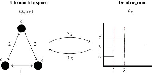
Figure 4: Transforming ultrametric spaces into dendrograms.

Theorem 14 (Dendrograms as ultrametric spaces, [7, Theorem 9]).

Given a finite set $X$, then $\Delta_{X}:\mathcal{U}(X)\rightarrow\mathcal{D}(X)$ is bijective with inverse $\Upsilon_{X}:\mathcal{D}(X)\rightarrow\mathcal{U}(X)$.

Theorem 14 above establishes that dendrograms and ultrametric spaces are equivalent concepts – a point of view which helps to formulate subsequent ideas in this paper.

Example 15 ($t$-closed/open quotient in terms of dendrograms).

It is helpful to understand both the open and closed $t$-quotients by viewing ultrametric spaces as dendrograms: both $t$-quotients simply forget the details of a given dendrogram strictly below scale $t$. Whereas the $t$-open equivalence relation retains the partition information at scale $t$, the $t$-closed equivalence does not. See Figure 5 for an illustration.

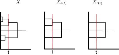
Figure 5: Illustration of open and closed equivalence relations. The leftmost figure is a dendrogram representing a 7-point ultrametric space $X$. The middle figure is the dendrogram corresponding to $X_{\mathfrak{o}(t)}$ whereas the rightmost figure is the dendrogram corresponding to $X_{\mathfrak{c}(t)}$.

3 Gromov-Hausdorff distances between ultrametric spaces

For convenience, we adopt the following notation to represent the absolute $p$-difference (for $p\in[1,\infty]$) between two non-negative numbers $a,b\in\mathbb{R}_{\geq 0}$:

$$\Lambda_{p}(a,b) \coloneqq|a^{p}-b^{p}|^{\frac{1}{p}}, \mbox{for }p\in[1,\infty);$$

$$\Lambda_{\infty}(a,b) \coloneqq\begin{cases}\max(a,b),&a\neq b\\ 0,&a=b\end{cases}, \mbox{for }p=\infty.$$

Note that $\Lambda_{1}(a,b)=|a-b|$ is the usual Euclidean distance and that $\lim_{p\rightarrow\infty}\Lambda_{p}(a,b)=\Lambda_{\infty}(a,b)$. In particular, for any $a,b\geq 0$, we have the following obvious characterization of $\Lambda_{\infty}(a,b)$:

$$\Lambda_{\infty}(a,b)=\inf\{c\geq 0:\,a\leq\max(b,c)\text{ and }b\leq\max(a,c)\}.$$ (7)

Proof.

We have the following two cases.

1. If $a=b$, then $\Lambda_{\infty}(a,b)=0\leq c.$

2. If $a\neq b$, we assume without loss of generality that $a>b$. Then, $a\leq\max(b,c)$ implies that $\Lambda_{\infty}(a,b)=\max(a,b)=a\leq c$.

∎

Now, given $p\in[1,\infty]$ and two ultrametric spaces $(X,u_{X})$ and $(Y,u_{Y})$, for any non-empty subset $S\subseteq X\times Y$, we define its $p$-distortion with respect to $u_{X}$ and $u_{Y}$ as follows:

$$\mathrm{dis}_{p}\left(S,u_{X},u_{Y}\right)\coloneqq\sup_{(x,y),(x^{\prime},y^{\prime})\in S}\Lambda_{p}(u_{X}(x,x^{\prime}),u_{Y}(y,y^{\prime})).$$ (8)

We abbreviate $\mathrm{dis}_{p}\left(S,u_{X},u_{Y}\right)$ to $\mathrm{dis}_{p}(S)$ whenever clear from the context. In particular, for a map $\varphi:X\rightarrow Y$, we define its $p$-distortion by

$$\mathrm{dis}_{p}(\varphi)\coloneqq\mathrm{dis}_{p}(\mathrm{graph}(\varphi))=\sup_{x,x^{\prime}\in X}\Lambda_{p}\big{(}u_{X}(x,x^{\prime}),u_{Y}(\varphi(x),\varphi(x^{\prime}))\big{)},$$

where $\mathrm{graph}(\varphi)\coloneqq\{(x,\varphi(x))\in X\times Y:\,x\in X\}$. Note that when $p=1$, we usually drop the subscript and simply write $\mathrm{dis}\coloneqq\mathrm{dis}_{1}$ and call the $1$-distortion simply the distortion.

Recall from the introduction that a correspondence $R$ between the underlying sets $X$ and $Y$ is any subset of $X\times Y$ such that the images of $R$ under the canonical projections $p_{X}:X\times Y\rightarrow X$ and $p_{Y}:X\times Y\rightarrow Y$ are full: $p_{X}(R)=X$ and $p_{Y}(R)=Y$.

Example 16.

Let $X=\{x_{1},x_{2}\}$ and $Y=\{y_{1},y_{2}\}$ be a pair of two-point spaces. Assume two ultrametrics $u_{X}$ and $u_{Y}$ on $X$ and $Y$, respectively, such that $u_{X}(x_{1},x_{2})=1$ and $u_{Y}(y_{1},y_{2})=2$. Let $R\coloneqq\{(x_{1},y_{1}),(x_{2},y_{2})\}$. Then, $R$ is a correspondence between $X$ and $Y$. For any $p\in[1,\infty]$, it is clear that

$$\mathrm{dis}_{p}(R,u_{X},u_{Y})=\Lambda_{p}\big{(}u_{X}(x_{1},x_{2}),u_{Y}(y_{1},y_{2})\big{)}=\begin{cases}|1^{p}-2^{p}|^{\frac{1}{p}}&p\in[1,\infty)\\ 2&p=\infty\end{cases}.$$

Now, for any $p\in[1,\infty]$, we define $d_{\mathrm{GH}}^{\scriptscriptstyle{(p)}}$ as follows, which is an extension of Equation (2) defined only for $p\in[1,\infty)$:

$$d_{\mathrm{GH}}^{\scriptscriptstyle{(p)}}(X,Y)\coloneqq 2^{-\frac{1}{p}}\inf_{R}\mathrm{dis}_{p}(R),$$ (9)

where the infimum is taken over all correspondences between $X$ and $Y$. Here we adopt the convention that $\frac{1}{\infty}=0$. Note that $d_{\mathrm{GH}}^{\scriptscriptstyle{(1)}}=d_{\mathrm{GH}}$, and as a consequence of our convention

$$d_{\mathrm{GH}}^{\scriptscriptstyle{(\infty)}}(X,Y)=\inf_{R}\mathrm{dis}_{\infty}(R).$$

As already mentioned in the introduction, when only considering finite ultrametric spaces, we easily have the following property of the family $\{d_{\mathrm{GH}}^{\scriptscriptstyle{(p)}}\}_{p\in[1,\infty]}$:

Proposition 17.

Given any $X,Y\in\mathcal{U}^{\mathrm{fin}}$, the function $p\mapsto d_{\mathrm{GH}}^{\scriptscriptstyle{(p)}}(X,Y)$ is continuous and increasing with respect to $p\in[1,\infty]$. In particular, $\lim_{p\rightarrow\infty}d_{\mathrm{GH}}^{\scriptscriptstyle{(p)}}(X,Y)=d_{\mathrm{GH}}^{\scriptscriptstyle{(\infty)}}(X,Y)$.

Remark 18.

Note that $d_{\mathrm{GH}}^{\scriptscriptstyle{(p)}}(X,Y)$ in Equation (9) is actually well-defined for any two metric spaces $X$ and $Y$, i.e., $X$ and $Y$ are not restricted to be ultrametric spaces. See Section 3.3 for alternative definitions of $d_{\mathrm{GH}}^{\scriptscriptstyle{(p)}}(X,Y)$ on classes of metric spaces larger than $\mathcal{U}$.

Example 19 (Distance to the one point space).

Since there exists a unique correspondence $R_{\ast}\coloneqq X\times\ast$ between a given finite set $X$ and the one point space $\ast$, we have for each $p\in[1,\infty]$ that

$$d_{\mathrm{GH}}^{\scriptscriptstyle{(p)}}(X,\ast)=2^{-\frac{1}{p}}\mathrm{dis}_{p}(R_{\ast})=2^{-\frac{1}{p}}\mathrm{diam}(X).$$

3.1 Computing $d_{\mathrm{GH}}^{\scriptscriptstyle{(p)}}$ is NP-hard when $p\in[1,\infty)$

Given an ultrametric space $(X,u_{X})$ and any positive real number $\alpha$, the function $(x,x^{\prime})\mapsto\left(u_{X}(x,x^{\prime})\right)^{\alpha}$ is still an ultrametric on $X$ so that the space $(X,(u_{X})^{\alpha})$ is still an ultrametric space. We let $S_{\alpha}(X)$ denote the ultrametric space $(X,(u_{X})^{\alpha})$. Then, we have the following transformation between $d_{\mathrm{GH}}^{\scriptscriptstyle{(p)}}$ and $d_{\mathrm{GH}}$ for all $p\in[1,\infty)$. The proof of the following result is relegated to Appendix C.

Proposition 20.

Given $1\leq p<\infty$ and any two ultrametric spaces $X$ and $Y$, one has

$$d_{\mathrm{GH}}^{\scriptscriptstyle{(p)}}(X,Y)=\big{(}d_{\mathrm{GH}}(S_{p}(X),S_{p}(Y))\big{)}^{\frac{1}{p}}.$$

Conversely,

$$d_{\mathrm{GH}}(X,Y)=\left(d_{\mathrm{GH}}^{\scriptscriptstyle{(p)}}\left(S_{\frac{1}{p}}(X),S_{\frac{1}{p}}(Y)\right)\right)^{p}.$$

Therefore, solving an instance of $d_{\mathrm{GH}}^{\scriptscriptstyle{(p)}}$ is equivalent to solving an instance of $d_{\mathrm{GH}}$. Since it is NP-hard to compute $d_{\mathrm{GH}}$ between finite ultrametric spaces [40], it is also NP-hard to compute $d_{\mathrm{GH}}^{\scriptscriptstyle{(p)}}$ between finite ultrametric spaces for every $p\in[1,\infty)$.

Moreover, combining Proposition 20 with Theorem 1, we have the following more precise statement: See 2

Proof.

Suppose otherwise that there exist ultrametric spaces $X$ and $Y$ such that $d_{\mathrm{GH}}^{\scriptscriptstyle{(p)}}(X,Y)$ can be approximated within a factor $c^{\frac{1}{p}}<3^{\frac{1}{p}}$ in polynomial time. Then, Proposition 20 implies that one can approximate $\big{(}d_{\mathrm{GH}}(S_{p}(X),S_{p}(Y))\big{)}^{\frac{1}{p}}$ within a factor $c^{\frac{1}{p}}<3^{\frac{1}{p}}$ in polynomial time. This implies that one can approximate $d_{\mathrm{GH}}(S_{p}(X),S_{p}(Y))$ within a factor $c<3$ in polynomial time which contradicts with Theorem 1. ∎

As mentioned in the introduction, the factor $3^{\frac{1}{p}}$ in Corollary 2 approaches $1$ as $p\rightarrow\infty$. This suggests that $d_{\mathrm{GH}}^{\scriptscriptstyle{(\infty)}}$ could be a computationally tractable quantity; later in Section 4.2 we will illustrate this point.

3.2 An estimate of $d_{\mathrm{GH}}^{\scriptscriptstyle{(p)}}$ via diameters of input spaces

The following result shows how the Gromov-Hausdorff distance interacts with the diameters of the input spaces.

Proposition 21 ([30, Theorems 3.3 and 3.4]).

For any finite metric spaces $X$ and $Y$, let $R$ be a correspondence between them. Then, we have

$$|\mathrm{diam}(X)-\mathrm{diam}(Y)|\leq\mathrm{dis}(R)\leq\max(\mathrm{diam}(X),\mathrm{diam}(Y)).$$

In particular,

$$\frac{1}{2}|\mathrm{diam}(X)-\mathrm{diam}(Y)|\leq d_{\mathrm{GH}}(X,Y)\leq\frac{1}{2}\max(\mathrm{diam}(X),\mathrm{diam}(Y)).$$

Invoking Proposition 20, we immediately have the following analogue to the second part of Proposition 21 for $d_{\mathrm{GH}}^{\scriptscriptstyle{(p)}}$:

Proposition 22.

For any $p\in[1,\infty)$ and finite ultrametric spaces $X$ and $Y$, we have that

$$2^{-\frac{1}{p}}\Lambda_{p}(\mathrm{diam}(X),\mathrm{diam}(Y))\leq d_{\mathrm{GH}}^{\scriptscriptstyle{(p)}}(X,Y)\leq 2^{-\frac{1}{p}}\max(\mathrm{diam}(X),\mathrm{diam}(Y)).$$

Note that $\lim_{p\rightarrow\infty}2^{-\frac{1}{p}}\Lambda_{p}(\mathrm{diam}(X),\mathrm{diam}(Y))=\Lambda_{\infty}(\mathrm{diam}(X),\mathrm{diam}(Y))$. When $\mathrm{diam}(X)\neq\mathrm{diam}(Y)$, $\lim_{p\rightarrow\infty}2^{-\frac{1}{p}}\Lambda_{p}(\mathrm{diam}(X),\mathrm{diam}(Y))=\max(\mathrm{diam}(X),\mathrm{diam}(Y))$. Then, by continuity of $d_{\mathrm{GH}}^{\scriptscriptstyle{(p)}}$ with respect to $p\in[1,\infty]$ (cf. Proposition 17), we have the following property for $d_{\mathrm{GH}}^{\scriptscriptstyle{(\infty)}}$:

Proposition 23.

Let $X$ and $Y$ be any two finite ultrametric spaces with different diameters, then

$$d_{\mathrm{GH}}^{\scriptscriptstyle{(\infty)}}(X,Y)=\max(\mathrm{diam}(X),\mathrm{diam}(Y)).$$

This proposition indicates that, when $X$ and $Y$ have different diameters, $d_{\mathrm{GH}}^{\scriptscriptstyle{(\infty)}}(X,Y)$ is determined by the diameter values of the input spaces, which suggests that $d_{\mathrm{GH}}^{\scriptscriptstyle{(\infty)}}$ is more rigid than other $d_{\mathrm{GH}}^{\scriptscriptstyle{(p)}}$ when $p<\infty$ and as a consequence, $d_{\mathrm{GH}}^{\scriptscriptstyle{(\infty)}}$ exhibits a distinct computational behavior in comparison to $d_{\mathrm{GH}}^{\scriptscriptstyle{(p)}}$ when $p<\infty$.

Example 24 (Distance between homothetic spaces).

Let $X$ be a finite ultrametric space and let $\lambda>0$. Then, for any $p\in[1,\infty]$ we have

$$d_{\mathrm{GH}}^{\scriptscriptstyle{(p)}}((X,u_{X}),(X,\lambda\cdot u_{X}))=2^{-\frac{1}{p}}\Lambda_{p}(\lambda,1)\cdot\mathrm{diam}(X).$$

Indeed, since $\mathrm{diam}(X,\lambda\cdot u_{X})=\lambda\cdot\mathrm{diam}(X)$, by Proposition 22 and Proposition 23 we have that

$$d_{\mathrm{GH}}^{\scriptscriptstyle{(p)}}((X,u_{X}),(X,\lambda\cdot u_{X}))\geq 2^{-\frac{1}{p}}\Lambda_{p}(\lambda\cdot\mathrm{diam}(X),\mathrm{diam}(X))=2^{-\frac{1}{p}}\Lambda_{p}(\lambda,1)\cdot\mathrm{diam}(X).$$

For the converse, consider the identity correspondence $R_{\mathrm{id}}\coloneqq\{(x,x)\in X\times X:x\in X\}$. Then,

$$d_{\mathrm{GH}}^{\scriptscriptstyle{(p)}}((X,u_{X}),(X,\lambda\cdot u_{X}))\leq 2^{-\frac{1}{p}}\mathrm{dis}_{p}\big{(}R_{\mathrm{id}},u_{X},\lambda\cdot u_{X}\big{)}=2^{-\frac{1}{p}}\Lambda_{p}(\lambda,1)\cdot\mathrm{diam}(X).$$

3.3 $d_{\mathrm{GH}}^{\scriptscriptstyle{(\infty)}}$ exactly coincides with the Gromov-Hausdorff ultrametric $u_{\mathrm{GH}}$

Recall that on a metric space $Z$, the Hausdorff distance $d_{\mathrm{H}}^{Z}$ between two subsets $A,B\subseteq Z$ is defined as

$$d_{\mathrm{H}}^{Z}(A,B):=\max\left(\sup_{a\in A}\inf_{b\in B}d_{Z}(a,b),\sup_{b\in B}\inf_{a\in A}d_{Z}(a,b)\right).$$

Given two metric spaces $X$ and $Y$, we say a map $\varphi:X\rightarrow Y$ is an isometric embedding from $X$ to $Y$ if for every $x,x^{\prime}\in X$, $d_{X}(x,x^{\prime})=d_{Y}(\varphi(x),\varphi(x^{\prime}))$. We usually use the symbol $\hookrightarrow$ (instead of $\rightarrow$) to represent isometric embeddings. Then, the Gromov-Hausdorff distance can be characterized as follows:

Theorem 25 (Duality formula for $d_{\mathrm{GH}}$, [6, Theorem 7.3.25]).

The Gromov-Hausdorff distance $d_{\mathrm{GH}}$ between two compact metric spaces $X$ and $Y$ satisfies the following:

$$d_{\mathrm{GH}}(X,Y)=\inf d^{Z}_{\mathrm{H}}(\varphi_{X}(X),\varphi_{Y}(Y)),$$ (10)

where the infimum is taken over all metric spaces $Z$ and isometric embeddings $\varphi_{X}:X\hookrightarrow Z$ and $\varphi_{Y}:Y\hookrightarrow Z$.

In fact, Equation (10) is the original definition of the Gromov-Hausdorff distance given by Gromov in [17]. In the spirit of Equation (10), Zarichnyi defines in [43] the Gromov-Hausdorff ultrametric, which we denote by $u_{\mathrm{GH}}$, between compact ultrametric spaces $X$ and $Y$ as follows:

$$u_{\mathrm{GH}}(X,Y):=\inf d^{Z}_{\mathrm{H}}(\varphi_{X}(X),\varphi_{Y}(Y)),$$

where the infimum is taken over all ultrametric spaces $Z$ and isometric embeddings $\varphi_{X}:X\hookrightarrow Z$ and $\varphi_{Y}:Y\hookrightarrow Z$. It turns out that $u_{\mathrm{GH}}$ agrees with $d_{\mathrm{GH}}^{\scriptscriptstyle{(\infty)}}$ as defined by Equation (9).

Theorem 26 (Duality formula for $d_{\mathrm{GH}}^{\scriptscriptstyle{(\infty)}}$).

Given two compact ultrametric spaces $X$ and $Y$, we have that

$$d_{\mathrm{GH}}^{\scriptscriptstyle{(\infty)}}(X,Y)=u_{\mathrm{GH}}(X,Y).$$ (11)

See Appendix C for the proof.

Zarichnyi proved in [43] that $u_{\mathrm{GH}}$ (and thus $d_{\mathrm{GH}}^{\scriptscriptstyle{(\infty)}}$) is an ultrametric on the collection of all compact ultrametric spaces. Similar metric properties also hold for $d_{\mathrm{GH}}^{\scriptscriptstyle{(p)}}$, for $p\in[1,\infty)$; see the following remark.

Remark 27 (Duality formula for $d_{\mathrm{GH}}^{\scriptscriptstyle{(p)}}$).

A similar alternative formulation via the Hausdorff distance exists for $d_{\mathrm{GH}}^{\scriptscriptstyle{(p)}}$ for each $p\in[1,\infty]$. For $p\in[1,\infty)$, we call a metric space $X$ a $p$-metric space if it satisfies the $p$-triangle inequality:

$$\forall x,x^{\prime},x^{\prime\prime}\in X,\,(d_{X}(x,x^{\prime}))^{p}\leq(d_{X}(x,x^{\prime\prime}))^{p}+(d_{X}(x^{\prime\prime},x^{\prime}))^{p}.$$

In that case, we refer to $d_{X}$ as a $p$-metric. Then, for any two compact $p$-metric spaces, we have that $d_{\mathrm{GH}}^{\scriptscriptstyle{(p)}}(X,Y)=\inf d^{Z}_{\mathrm{H}}(\varphi(X),\varphi_{Y}(Y)),$ where the infimum is taken over all $p$-metric spaces $Z$ and isometric embeddings $\varphi_{X}:X\hookrightarrow Z$ and $\varphi_{Y}:Y\hookrightarrow Z$. Moreover, $d_{\mathrm{GH}}^{\scriptscriptstyle{(p)}}$ is actually a $p$-metric on the collection of isometry classes of compact $p$-metric spaces. We do not provide details here; see our technical report [31] for these.

4 Structural results for $u_{\mathrm{GH}}$ and computational implications

In this section, we first prove our central observation regarding $u_{\mathrm{GH}}$, the structural theorem for $u_{\mathrm{GH}}$ (Theorem 3). Then, we utilize this theorem to devise a poly-time algorithm for computing $u_{\mathrm{GH}}$. We remark that the distance $u_{\mathrm{GH}}$ as well as Theorem 3 and Algorithm 1 can be extended to the so-called ultra-dissimilarity spaces, which can be regarded as generalization of ultrametric spaces. See Appendix B for details.

4.1 Proof of Theorem 3

Recall the statement of the structural theorem for $u_{\mathrm{GH}}$: See 3

Proof.

We first prove the following weaker version of Theorem 3 (with $\inf$ instead of $\min$):

$$u_{\mathrm{GH}}(X,Y)=\inf\left\{t\geq 0:\,\left(X_{\mathfrak{c}(t)},u_{X_{\mathfrak{c}(t)}}\right)\cong\left(Y_{\mathfrak{c}(t)},u_{Y_{\mathfrak{c}(t)}}\right)\right\}.$$ (12)

Suppose first that $X_{\mathfrak{c}(t)}\cong Y_{\mathfrak{c}(t)}$ for some $t\geq 0$, i.e. there exists an isometry $f_{t}:X_{\mathfrak{c}(t)}\rightarrow Y_{\mathfrak{c}(t)}$. Define

$$R_{t}\coloneqq\left\{(x,y)\in X\times Y:\,[y]_{\mathfrak{c}(t)}^{Y}=f_{t}\left([x]^{X}_{\mathfrak{c}(t)}\right)\right\}.$$

That $R_{t}$ is a correspondence between $X$ and $Y$ is clear since: $f_{t}$ is bijective, every $x\in X$ belongs to exactly one block in $X_{\mathfrak{c}(t)}$ and every $y\in Y$ belongs to exactly one block in $Y_{\mathfrak{c}(t)}$. For any $(x,y),(x^{\prime},y^{\prime})\in R_{t}$, if $u_{X}(x,x^{\prime})\leq t$, then we already have $u_{X}(x,x^{\prime})\leq\max(t,u_{Y}(y,y^{\prime}))$. Otherwise, if $u_{X}(x,x^{\prime})>t$, then we have $[x]^{X}_{\mathfrak{c}(t)}\neq[x^{\prime}]^{X}_{\mathfrak{c}(t)}$. Since $f_{t}$ is bijective, we have that $[y]^{Y}_{\mathfrak{c}(t)}=f_{t}([x]^{X}_{\mathfrak{c}(t)})\neq f_{t}([x^{\prime}]^{X}_{\mathfrak{c}(t)})=[y^{\prime}]^{Y}_{\mathfrak{c}(t)}.$ Then,

$$u_{Y}(y,y^{\prime})=u_{Y_{\mathfrak{c}(t)}}\left([y]^{Y}_{\mathfrak{c}(t)},[y^{\prime}]^{Y}_{\mathfrak{c}(t)}\right)=u_{X_{\mathfrak{c}(t)}}\left([x]^{X}_{\mathfrak{c}(t)},[x^{\prime}]^{X}_{\mathfrak{c}(t)}\right)=u_{X}(x,x^{\prime}).$$

Therefore, $u_{X}(x,x^{\prime})\leq\max(t,u_{Y}(y,y^{\prime}))$. Similarly, $u_{Y}(y,y^{\prime})\leq\max(t,u_{X}(x,x^{\prime}))$. Then, by Equation (7), $\Lambda_{\infty}(u_{X}(x,x^{\prime}),u_{Y}(y,y^{\prime}))\leq t$ and thus $\mathrm{dis}_{\infty}(R_{t})\leq t$. This implies that

$$u_{\mathrm{GH}}(X,Y)\leq\inf\left\{t\geq 0:\,X_{\mathfrak{c}(t)}\cong Y_{\mathfrak{c}(t)}\right\}.$$

Conversely, let $R$ be any correspondence between $X$ an $Y$ and let $t\coloneqq\mathrm{dis}_{\infty}(R)$. Consider any $(x,y),(x^{\prime},y^{\prime})\in R$ such that $[x^{\prime}]^{X}_{\mathfrak{c}(t)}=[x]^{X}_{\mathfrak{c}(t)}$ (i.e. $u_{X}(x^{\prime},x)\leq t$). We define a map $f_{t}:X_{\mathfrak{c}(t)}\rightarrow Y_{\mathfrak{c}(t)}$ as follows: for each $[x]_{\mathfrak{c}(t)}^{X}\in X_{\mathfrak{c}(t)}$, suppose $y\in Y$ is such that $(x,y)\in R$, then we let $f_{t}\left([x]_{\mathfrak{c}(t)}^{X}\right)\coloneqq[y]_{\mathfrak{c}(t)}^{Y}$.

$f_{t}$ is well-defined. Indeed, if $[x]_{\mathfrak{c}(t)}^{X}=[x^{\prime}]_{\mathfrak{c}(t)}^{X}$ and $y,y^{\prime}\in Y$ are such that $(x,y),(x^{\prime},y^{\prime})\in R$, then

$$\Lambda_{\infty}(u_{X}(x,x^{\prime}),u_{Y}(y,y^{\prime}))\leq\mathrm{dis}_{\infty}(R)=t.$$

This implies that $u_{Y}(y^{\prime},y)\leq t$ which is equivalent to $[y]^{Y}_{\mathfrak{c}(t)}=[y^{\prime}]^{Y}_{\mathfrak{c}(t)}$. Similarly, there is a well-defined map $g_{t}:Y_{\mathfrak{c}(t)}\rightarrow X_{\mathfrak{c}(t)}$ sending $[y]_{\mathfrak{c}(t)}^{Y}\in Y_{\mathfrak{c}(t)}$ to $[x]_{\mathfrak{c}(t)}^{X}$ whenever $(x,y)\in R$. It is clear that $g_{t}$ is the inverse of $f_{t}$ and thus $f_{t}$ is bijective. Now suppose that $u_{X_{\mathfrak{c}(t)}}\left([x]^{X}_{\mathfrak{c}(t)},[x^{\prime}]^{X}_{\mathfrak{c}(t)}\right)=s>t$, which implies that $u_{X}(x,x^{\prime})=s$. Let $y,y^{\prime}\in Y$ be such that $(x,y),(x^{\prime},y^{\prime})\in R$. Then, since $\Lambda_{\infty}(u_{X}(x,x^{\prime}),u_{Y}(y,y^{\prime}))\leq\mathrm{dis}_{\infty}(R)=t<s$, $u_{Y}(y,y^{\prime})$ is forced to be equal to $u_{X}(x,x^{\prime})=s$. Therefore,

$$u_{Y_{\mathfrak{c}(t)}}\left(f_{t}\left([x]^{X}_{\mathfrak{c}(t)}\right),f_{t}\left([x^{\prime}]^{X}_{\mathfrak{c}(t)}\right)\right)=u_{Y_{\mathfrak{c}(t)}}\left([y]^{Y}_{\mathfrak{c}(t)},[y^{\prime}]^{Y}_{\mathfrak{c}(t)}\right)=s=u_{X_{\mathfrak{c}(t)}}\left([x]^{X}_{\mathfrak{c}(t)},[x^{\prime}]^{X}_{\mathfrak{c}(t)}\right).$$

This proves that $f_{t}$ is an isometry and thus

$$u_{\mathrm{GH}}(X,Y)\geq\inf\left\{t\geq 0:\,X_{\mathfrak{c}(t)}\cong Y_{\mathfrak{c}(t)}\right\}.$$

Since $X$ and $Y$ are finite, for each $t\geq 0$, there exists $\varepsilon>0$ such that for all $s\in[t,t+\varepsilon]$ $X_{\mathfrak{c}(t)}\cong X_{\mathfrak{c}(s)}$ and $Y_{\mathfrak{c}(t)}\cong Y_{\mathfrak{c}(s)}$. This implies that the infimum in Equation (12) is attained and thus we obtain the claim. ∎

Remark 28.

Theorem 3 actually holds for compact ultrametric spaces; see our technical report [31] for details.

4.2 A poly-time algorithm for computing $u_{\mathrm{GH}}$

In Algorithm 1 below we provide pseudocode for computing $u_{\mathrm{GH}}$ and in Theorem 29 we prove that Algorithm 1 runs in time $O(n^{2})$; see also Remark 30 for details about improving this time complexity to $O(n\log(n))$.

Recall that the spectrum $\mathrm{spec}(X)$ of the metric space $X$ is the set of values defined by $\mathrm{spec}(X)\coloneqq\{u_{X}(x,x^{\prime}):\,\forall x,x^{\prime}\in X\}$. The pseudocode for the function $\mathbf{ClosedQuotient}$ implementing the closed quotient operation is given in Algorithm 6 in Appendix A. The function $\mathbf{is\_iso}$ determines whether two ultrametric spaces are isometric, for which we adapt the algorithm in [3, Example 3.2].

Algorithm 1 $\mathbf{uGH}(X,Y)$

1:  $\mathrm{spec}\leftarrow$ sort($\mathrm{spec}(X)\cup\mathrm{spec}(Y)$, ‘descend’)

2:  for $i=1:\mathrm{length(spec)}$ do

3:     $t=\mathrm{spec}(i)$

4:     if $\thicksim\mathbf{is\_iso}(\mathbf{ClosedQuotient}(X,t),\mathbf{ClosedQuotient}(Y,t))$ then

5:        return  $\mathrm{spec}(i-1)$

6:     end if

7:  end for

8:  return  $0$

Complexity analysis of Algorithm 1

Let $n\coloneqq\max(\#X,\#Y)$. By Proposition 7, $\#\mathrm{spec}(X)\leq\#X$. Then,

$$\#\mathrm{spec}=\#\left(\mathrm{spec}(X)\bigcup\mathrm{spec}(Y)\right)=O(n).$$

Thus, it takes time $O(n\log(n))$ to construct and to sort the sequence $\mathrm{spec}\coloneqq\mathrm{spec}(X)\bigcup\mathrm{spec}(Y)$ (cf. Lemma 67). Now, for each $t\in\mathrm{spec}$, we need time $O(n)$ for running Algorithm $\mathbf{ClosedQuotient}$ (Algorithm 6) with input $(X,t)$ and $(Y,t)$.

Following Appendix A and Lemma 68, since $\max(\#X_{\mathfrak{c}(t)},\#Y_{\mathfrak{c}(t)})\leq\max(\#X,\#Y)=O(n)$, the function $\mathbf{is\_iso}$ with input $(X_{\mathfrak{c}(t)},Y_{\mathfrak{c}(t)})$ runs in time $O(n)$ as well (cf. Lemma 68).

Thus, the time complexity associated to computing $u_{\mathrm{GH}}(X,Y)$ via Algorithm 1 is

$$O(n\log(n))+\mathrm{length(spec)}\cdot O(n)=O(n\log(n))+O(n)\cdot O(n)=O(n^{2}).$$

In this way we have proved the following theorem.

Theorem 29 (Time complexity of Algorithm $\mathbf{uGH}$ (Algorithm 1)).

Let $X$ and $Y$ be finite ultrametric spaces. Then, algorithm $\mathbf{uGH}(X,Y)$ (Algorithm 1) runs in time $O\left(n^{2}\right)$, where $n\coloneqq\max(\#X,\#Y)$.

Remark 30 (Acceleration via binary search).

By replacing the for-loop over $i=1:\mathrm{length(spec)}$ in $\mathbf{uGH}$ (Algorithm 1) with binary search, the total complexity will drop to $O(n\log(n))+O(\log(n))\cdot O(n)=O(n\log(n)).$

Remark 31 (A novel poly time solvable instance of the quadratic assignment problem).

Given $p\in[1,\infty]$ and two finite ultrametric spaces $X=\{x_{1},\ldots,x_{n_{X}}\}$ and $Y=\{y_{1},\ldots,y_{n_{Y}}\}$, we formulate the computation of $d_{\mathrm{GH}}^{\scriptscriptstyle{(p)}}(X,Y)$ as the following generalized bottleneck quadratic assignment problem ($\mathrm{GQBAP}_{p}$) as in [30, Remark 3.4] (cf. Equation (9)):

$$\mathrm{GQBAP}_{p}(\mathbf{a},\mathbf{b})\coloneqq 2^{\frac{1}{p}}\,d_{\mathrm{GH}}^{\scriptscriptstyle{(p)}}(X,Y)=\min_{R}\max_{i,j,k,l}\Lambda_{p}(a_{ik},b_{jl})\,R_{ij}\,R_{kl},$$

where $\mathbf{a}=(a_{ik})$ is an $n_{X}\times n_{X}$ matrix such that $a_{ik}\coloneqq u_{X}(x_{i},x_{k})$, $\mathbf{b}=(b_{jl})$ is an $n_{Y}\times n_{Y}$ matrix such that $b_{jl}\coloneqq u_{Y}(y_{j},y_{l})$, and $R$ is a correspondence, which is regarded as $(R_{ij})$, an $n_{X}\times n_{Y}$ matrix such that $R_{ij}\in\{0,1\}$ and

1. $\sum_{i=1}^{n_{X}}R_{ij}\geq 1$ for all $j$;

2. $\sum_{j=1}^{n_{Y}}R_{ij}\geq 1$ for all $i$.

Then, by Corollary 2 and Theorem 29, whereas solving $\mathrm{GQBAP}_{p}$ is NP-hard for each $p\in[1,\infty)$, the problem $\mathrm{GQBAP}_{\infty}$ can be solved in time $O(n\log(n))$ where $n\coloneqq\max(n_{X},n_{Y})$.

In general, quadratic assignment problems are NP-hard [34]. This includes instances such as $\mathrm{GQBAP}_{p}$ in the case when $p<\infty$. However, by the above ‘cost’ matrices of the form of $\left(\Lambda_{\infty}(a_{ik},b_{jl})\right)$ yield computationally tractable instances.

5 Structural results for $d_{\mathrm{GH}}$ and computational implications

In this section, we first prove the structural theorem for $d_{\mathrm{GH}}$ (Theorem 4), and then develop efficient algorithms for computing $d_{\mathrm{GH}}$ based on Theorem 4.

5.1 Proof of Theorem 4

Recall the structural theorem for the Gromov-Hausdorff distance:

See 4

Proof.

First suppose that there exists an $\varepsilon$-correspondence $R$ between $X$ and $Y$. Then, we define a map $\Psi:[N_{X}]\rightarrow[N_{Y}]$ as follows: for any $i\in[N_{X}]$, pick an arbitrary $x\in X_{i}$ and assume that $(x,y)\in R$ for some $y\in Y$; further assume that $y\in Y_{j}$ for some $j\in[N_{Y}]$, then we let $\Psi(i)\coloneqq j$. Now, we verify that this map $\Psi$ is well-defined, i.e., $\Psi$ is independent of choice of $x\in X_{i}$ and choice of $(x,y)\in R$. For any $i\in[N_{X}]$ and $x,x^{\prime}\in X_{i}$, we have by assumption that $u_{X}(x,x^{\prime})<\delta_{\varepsilon}(Y)$. Suppose $y,y^{\prime}\in Y$ are such that $(x,y),(x^{\prime},y^{\prime})\in R$. Then,

$$u_{Y}(y,y^{\prime})\leq u_{X}(x,x^{\prime})+\mathrm{dis}(R)\leq u_{X}(x,x^{\prime})+\varepsilon<\delta_{\varepsilon}(Y)+\varepsilon=\delta_{0}(Y).$$

Therefore, there exists a common $j\in[N_{Y}]$ such that both $y\in Y_{j}$ and $y^{\prime}\in Y_{j}$. This implies that $\Psi$ is well-defined. Since $R$ is a correspondence, $\Psi$ must be surjective. Then, for each $j\in[N_{Y}]$, we define the set

$$R_{j}\coloneqq R\bigcap(X_{\Psi^{-1}(j)}\times Y_{j})$$

It is obvious that $R_{j}$ is a correspondence between $X_{\Psi^{-1}(j)}$ and $Y_{j}$. Moreover, $\mathrm{dis}(R_{j})\leq\mathrm{dis}(R)\leq\varepsilon$ for each $j\in[N_{Y}]$. Therefore, for each $j\in[N_{Y}]$, $R_{j}$ is an $\varepsilon$-correspondence between $X_{\Psi^{-1}(j)}$ and $Y_{j}$.

Conversely, suppose that there exist a surjection $\Psi:[N_{X}]\twoheadrightarrow[N_{Y}]$ and for each $j\in[N_{Y}]$ an $\varepsilon$-correspondence $R_{j}$ between $X_{\Psi^{-1}(j)}$ and $Y_{j}$. Then, define $R\coloneqq\bigcup_{j\in[N_{Y}]}R_{j}.$ It is clear that $R$ is a correspondence between $X$ and $Y$ because

$$p_{X}\left(\bigcup_{j\in[N_{Y}]}R_{j}\right)=\bigcup_{j\in[N_{Y}]}p_{X}(R_{j})=\bigcup_{j\in[N_{Y}]}X_{\Psi^{-1}(j)}=X$$

and

$$p_{Y}\left(\bigcup_{j\in[N_{Y}]}R_{j}\right)=\bigcup_{j\in[N_{Y}]}p_{Y}(R_{j})=\bigcup_{j\in[N_{Y}]}Y_{j}=Y,$$

where $p_{X}:X\times Y\rightarrow X$ and $p_{Y}:X\times Y\rightarrow Y$ are the canonical coordinate projections. Given any $(x,y),(x^{\prime},y^{\prime})\in R$, suppose $(x,y)\in R_{j}$ and $(x^{\prime},y^{\prime})\in R_{j^{\prime}}$ for some $j,j^{\prime}\in[N_{Y}]$. Then, we verify that $|u_{X}(x,x^{\prime})-u_{Y}(y,y^{\prime})|\leq\varepsilon$ in the following two cases:

1. if $j=j^{\prime}$, then $|u_{X}(x,x^{\prime})-u_{Y}(y,y^{\prime})|\leq\mathrm{dis}(R_{j})\leq\varepsilon;$

2. if $j\neq j^{\prime}$, then $x$ and $x^{\prime}$ belong to different blocks of $X_{\mathfrak{o}\left(\delta_{\varepsilon}(Y)\right)}$, and $y$ and $y^{\prime}$ belong to different blocks of $Y_{\mathfrak{o}\left(\delta_{0}(Y)\right)}$. Then, $u_{X}(x,x^{\prime})\geq\delta_{\varepsilon}(Y)=\mathrm{diam}(Y)-\varepsilon$ and $u_{Y}(y,y^{\prime})=\delta_{0}(Y)=\mathrm{diam}(Y)$. So, $u_{X}(x,x^{\prime})\geq u_{Y}(y,y^{\prime})-\varepsilon$. By the assumption that $|\mathrm{diam}(X)-\mathrm{diam}(Y)|\leq\varepsilon$, we have that $u_{X}(x,x^{\prime})\leq\mathrm{diam}(X)\leq\mathrm{diam}(Y)+\varepsilon=u_{Y}(y,y^{\prime})+\varepsilon$. Therefore, $|u_{X}(x,x^{\prime})-u_{Y}(y,y^{\prime})|\leq\varepsilon.$

Therefore, $\mathrm{dis}(R)\leq\varepsilon$ and thus $R$ is an $\varepsilon$-correspondence between $X$ and $Y$. This also proves Remark 6. ∎

5.2 Algorithms for computing $d_{\mathrm{GH}}$ based on Theorem 4

The main goal of this section is to develop an efficient algorithm for computing the exact value of $d_{\mathrm{GH}}$ between ultrametric spaces. To achieve the goal, we first consider the following decision problem:

Decision Problem GHDU-dec ($d_{\mathrm{GH}}$ distance computation between finite ultrametric spaces)

Inputs: Finite ultrametric spaces $X$ and $Y$, as well as $\varepsilon\geq 0$.

Question: Is there an $\varepsilon$-correspondence between $X$ and $Y$?

5.2.1 Strategy for solving GHDU-dec

Base cases for Problem GHDU-dec

Proposition 21 shows how the Gromov-Hausdorff distance $d_{\mathrm{GH}}$ interacts with the diameters of the input spaces. This theorem then implies that GHDU-dec is solved immediately in the following two base cases:

Base Case 1:

If $|\mathrm{diam}(X)-\mathrm{diam}(Y)|>\varepsilon$, then there exists no $\varepsilon$-correspondence between $X$ and $Y$.

Base Case 2:

If $\max(\mathrm{diam}(X),\mathrm{diam}(Y))\leq\varepsilon$, then every correspondence $R$ between $X$ and $Y$ is an $\varepsilon$-correspondence.

Base Case 1 justifies our assumption that $|\mathrm{diam}(X)-\mathrm{diam}(Y)|\leq\varepsilon$ in Theorem 4 since otherwise we would be in one of the two base cases. Note that the situation when one of the two spaces is the one point space will automatically fall in either of the above two base cases.

Application of Theorem 4

Suppose that we are given two ultrametric spaces $X$ and $Y$ and $\varepsilon\geq 0$ not falling in either of the two base cases mentioned above. This implies that one of $\mathrm{diam}(X)$ or $\mathrm{diam}(Y)$ must be strictly larger than $\varepsilon$.

Suppose $\mathrm{diam}(Y)>\varepsilon$ (otherwise we swap the roles of $X$ and $Y$) and apply the open partition operation to $X$ and $Y$ to obtain $X_{\mathfrak{o}\left(\delta_{\varepsilon}(Y)\right)}:=\{X_{i}\}_{i\in[N_{X}]}$ and $Y_{\mathfrak{o}\left(\delta_{0}(Y)\right)}:=\{Y_{j}\}_{j\in[N_{Y}]}$. Here we use the same notation as in Theorem 4 that for each $i\in[N_{X}]$, $X_{i}$ denotes an open equivalence class $[x_{i}]_{\mathfrak{o}(\delta_{\varepsilon}(Y))}$ for some $x_{i}\in X$ and similarly for notation $Y_{j}$.

If there is no surjection from $[N_{X}]$ to $[N_{Y}]$, i.e., $N_{X}<N_{Y}$, then we conclude from Theorem 4 that there is no $\varepsilon$-correspondence between $X$ and $Y$. Otherwise, for each surjection $\Psi:[N_{X}]\twoheadrightarrow[N_{Y}]$ and for each $j\in[N_{Y}]$, we solve one instance of the decision problem GHDU-dec with input $(X_{\Psi^{-1}(j)},Y_{j},\varepsilon)$. If for some surjection $\Psi$, there exist $\varepsilon$-correspondences $R_{j}$ between $X_{\Psi^{-1}(j)}$ and $Y_{j}$ for all $j\in[N_{Y}]$, then the union of all $R_{j}$s is an $\varepsilon$-correspondence between $X$ and $Y$ (cf. Remark 6). Otherwise, by Theorem 4 again, there exists no $\varepsilon$-correspondence between $X$ and $Y$.

For each pair $(X_{\Psi^{-1}(j)},Y_{j})$ as described above, it is easy to see that $\#X_{\Psi^{-1}(j)}<\#X$ and $\#Y_{j}<\#Y$. So, if we repeatedly apply the open partition operation as in Theorem 4, we will eventually reduce the problem to one of the two base cases.

5.2.2 A recursive algorithm

From the analysis above we identify a recursive algorithm $\mathbf{FindCorrRec}$ (Algorithm 2) which takes as input two ultrametric spaces $X$ and $Y$ and a parameter $\varepsilon\geq 0$. If there exists an $\varepsilon$-correspondence between $X$ and $Y$, then $\mathbf{FindCorrRec}(X,Y,\varepsilon)$ returns such an $\varepsilon$-correspondence. If there exists no $\varepsilon$-correspondence, $\mathbf{FindCorrRec}(X,Y,\varepsilon)$ returns 0.

Algorithm 2 $\mathbf{FindCorrRec}(X,Y,\varepsilon)$

1:  BoolSwap $\leftarrow$ FALSE

2:  if $\mathrm{diam}(X)>\mathrm{diam}(Y)$ then

3:     Swap $X$ and $Y$; BoolSwap $\leftarrow$ TRUE

4:  end if

5:  if $\max\left(\mathrm{diam}(X),\mathrm{diam}(Y)\right)\leq\varepsilon$ then

6:     $R\leftarrow\mathrm{ones}\left({\#X,\#Y}\right)$

7:  end if

8:  if BoolSwap then

9:     Transpose $R$

10:     return  $R$

11:  end if

12:  if  $|\mathrm{diam}(X)-\mathrm{diam}(Y)|>\varepsilon$ then

13:     return  0

14:  end if

15:  $\{X_{i}\}_{i\in[N_{X}]}=\mathbf{OpenPartition}(X,\delta_{\varepsilon}(Y))$

16:  $\{Y_{j}\}_{j\in[N_{Y}]}=\mathbf{OpenPartition}(Y,\delta_{0}(Y))$

17:  for Each surjection $\Psi:[N_{X}]\twoheadrightarrow[N_{Y}]$ do

18:     for $j\in[N_{Y}]$ do

19:        $R_{j}\leftarrow\mathbf{FindCorrRec}\left(X_{\Psi^{-1}(j)},Y_{j},\varepsilon\right)$

20:        if $\left(\left(R_{j}\,!=0\right)\forall j\right)$ then

21:           $R\leftarrow\bigcup_{j=1}^{N_{Y}}R_{j}$

22:           if BoolSwap then

23:              Transpose $R$

24:           end if

25:           return  $R$

26:        end if

27:     end for

28:  end for

29:  return  0

Complexity analysis

To analyze the complexity of this recursive algorithm, we need to control the size of subproblems, i.e., the sizes of the blocks of the partitions produced by the open equivalence relations. The following structural condition on ultrametric spaces serves this purpose.

Definition 32 (First $(\varepsilon,\gamma)$-growth condition).

For $\varepsilon\geq 0$, and $\gamma>1$, we say that an ultrametric space $(X,u_{X})$ satisfies the first $(\varepsilon,\gamma)$-growth condition (FGC) if for all $x\in X$, and $t\geq\varepsilon$,

$${\#[x]_{\mathfrak{c}\left(t\right)}}\leq\gamma\cdot{\#[x]_{\mathfrak{o}\left(t-\varepsilon\right)}}.$$

Note that on the left-hand side of the inequality above we consider a ‘closed’ equivalence class whereas on the right-hand side we consider an ‘open’ equivalence class. We denote by $\mathcal{U}_{1}(\varepsilon,\gamma)$ the collection of all finite ultrametric spaces satisfying the first $(\varepsilon,\gamma)$-growth condition. See Figure 6 for an illustration and Remark 33 for an interpretation.

Figure 6: Illustration of Definition 32. $X$ and $Y$ are two 4-point ultrametric spaces. Suppose $s=t-\varepsilon$ for some $\varepsilon>0$. It is easy to see that $Y\in\mathcal{U}(\varepsilon,2)$. Since $2\,\#[x_{4}]_{\mathfrak{o}\left(s\right)}=2<4=\#[x_{4}]_{\mathfrak{o}\left(t\right)}$, it is easy to see that, in contrast, $X\notin\mathcal{U}(\varepsilon,2)$. This example illustrates that the FGC prevents a given equivalence class in $X_{\mathfrak{o}(t)}$ from containing most of the points of $X$ and thus its dendrogram will tend to split ‘evenly’.

Remark 33 (Interpretation of the FGC).

The main idea behind the first $(\varepsilon,\gamma)$-growth condition is that for each $t>0$ we want to have some degree of control over both the cardinalities of and the number of descendants of each $[x]_{\mathfrak{c}(t)}$ in $X_{\mathfrak{c}(t)}$, where we say that $[x^{\prime}]_{\mathfrak{o}\left(s\right)}$ is an (open) descendant of $[x]_{\mathfrak{c}(t)}$, or conversely that $[x]_{\mathfrak{c}(t)}$ is a (closed) ancestor of $[x^{\prime}]_{\mathfrak{o}\left(s\right)}$, if $[x^{\prime}]_{\mathfrak{o}\left(s\right)}\subseteq[x]_{\mathfrak{c}(t)}$.

More precisely, we write explicitly the $(t-\varepsilon)$-open partition of $[x]_{\mathfrak{c}(t)}$ by $[x]_{\mathfrak{c}\left(t\right)}=\sqcup_{i=1}^{N}[x_{i}]_{\mathfrak{o}\left(t-\varepsilon\right)}$ for some $x_{i}\in[x]_{\mathfrak{c}(t)}$, $i=1,\ldots,N$.

First, we note that $[x]_{\mathfrak{c}\left(t\right)}=[x_{i}]_{\mathfrak{c}\left(t\right)}$ for each $i=1,\ldots,N$ and thus the FGC implies that

$${\#[x_{i}]_{\mathfrak{o}\left(t-\varepsilon\right)}}\geq\frac{\#[x_{i}]_{\mathfrak{c}\left(t\right)}}{\gamma}=\frac{\#[x]_{\mathfrak{c}\left(t\right)}}{\gamma}.$$

This means that each descendant at scale $t-\varepsilon$ of a given block $[x]_{\mathfrak{c}\left(t\right)}$ contains at least a fixed proportion $\frac{1}{\gamma}$ of the number of points in its ancestor $[x]_{\mathfrak{c}\left(t\right)}$.

Moreover, we have

$$\#[x]_{\mathfrak{c}\left(t\right)}=\sum_{i=1}^{N}\#[x_{i}]_{\mathfrak{o}\left(t-\varepsilon\right)}\geq\frac{N}{\gamma}\#[x]_{\mathfrak{c}\left(t\right)}.$$

Therefore $N\leq\gamma$, which implies that each $[x]_{\mathfrak{c}\left(t\right)}$ has at most $\gamma$ many descendants at scale $t-\varepsilon$.

By invoking the master theorem [12] we now prove the following theorem which provides an upper bound on the complexity of Algorithm 2. See Section C.2.1 for its proof.

Theorem 34 (Time complexity of Algorithm $\mathbf{FindCorrRec}$ (Algorithm 2)).

Fix some $\varepsilon\geq 0$ and $\gamma\geq 2$. Then, for any $X,Y\in\mathcal{U}_{1}(\varepsilon,\gamma)$, $\mathbf{FindCorrRec}(X,Y,\varepsilon)$ (Algorithm 2) runs in time $O\left(n^{(\gamma+1)\log_{\mathrm{b}(\gamma)}\gamma}\right)$, where $n:=\max(\#X,\#Y)$ and $\mathrm{b}(\gamma):=\frac{\gamma^{2}}{\gamma^{2}-1}$.

Under the FGC, our recursive algorithm $\mathbf{FindCorrRec}$ (Algorithm 2) exhibits time complexity $O\left(n^{(\gamma+1)\log_{\mathrm{b}(\gamma)}\gamma}\right)$. Since the exponent of $n$ depends on $\gamma$, this is only partially satisfactory. In other words, Algorithm 2 is not yet fixed-parameter tractable, a notion which requires the exponent to be independent of the parameters involved. This motivates us to further examine and improve Algorithm 2 in order to develop an FPT algorithm. Note that in the for-loop over surjections in Algorithm 2, for different surjections $\Psi_{1},\Psi_{2}:[N_{X}]\twoheadrightarrow[N_{Y}]$, there could be some $j_{0}\in[N_{Y}]$ such that $\Psi^{-1}_{1}(j_{0})=\Psi^{-1}_{2}(j_{0})$. This would result in repetitive computations of $\mathbf{FindCorrRec}\left(X_{\Psi^{-1}_{1}(j_{0})},Y_{j_{0}},\varepsilon\right)$. With the goal of eliminating such repetitions, in the next section we devise a dynamic programming algorithm which eventually turns out to be FPT.

5.2.3 A dynamic programming algorithm

In this section, we introduce a dynamic programming algorithm $\mathbf{FindCorrDP}$ for solving the decision problem GHDU-dec for which we provide pseudocode in Algorithm 4. To proceed with the description of Algorithm 4, we first introduce some notation.

We let $V_{X}$ denote the set of all closed balls in $X$. For each closed ball $B\in V_{X}$, let $\rho_{\varepsilon}\left(B\right)\coloneqq\max(\mathrm{diam}\left(B\right)-2\varepsilon,0)$ and write the $\rho_{\varepsilon}\left(B\right)$-open partition of $B$ as:

$$B_{\mathfrak{o}\left(\rho_{\varepsilon}\left(B\right)\right)}:=\left\{[x_{i}]_{\mathfrak{o}\left(\rho_{\varepsilon}(B)\right)}^{B}\right\}_{i=1}^{N_{B}}$$

where $x_{i}\in B$ for $i=1,\ldots,N_{B_{X}}$. For notational simplicity, we let $B_{i}\coloneqq[x_{i}]_{\mathfrak{o}\left(\rho_{\varepsilon}(B)\right)}^{B}$ for each $i=1,\ldots,N_{B}$. It is obvious that each $[x]_{\mathfrak{o}\left(\rho_{\varepsilon}(B)\right)}^{B}=[x]_{\mathfrak{o}\left(\rho_{\varepsilon}(B)\right)}^{X}$ is actually a closed ball in $X$. Then, $B_{i}\in V_{X}$ for all $i=1,\ldots,N_{B}$. Note that for any $I\subseteq\{1,\ldots,N_{B}\}$, $\mathrm{diam}(\bigcup_{i\in I}B_{i})\leq\mathrm{diam}\left(B\right).$ If the equality is achieved, we call $\bigcup_{i\in I}B_{i}$ an $\varepsilon$-maximal union of closed balls of $B$. Denote by $B_{(\varepsilon)}$ the set of all $\varepsilon$-maximal unions of closed balls in $B$. Then, define a new set $V_{X}^{(\varepsilon)}\coloneqq\bigcup_{B\in V_{X}}B_{(\varepsilon)}$ by replacing each $B\in V_{X}$ with the set $B_{(\varepsilon)}$. We use the notation $U^{X}$ to represent a generic element in $V_{X}^{(\varepsilon)}$. See Figure 7 for an illustration of $V_{X}^{(\varepsilon)}$.

Figure 7: Illustration of $V_{X}^{(\varepsilon)}$ from Section 5.2.3. Note that $V_{X}=\{\{a\},\{b\},\{c\},\{a,b\},\{a,b,c\}\}$. For the ball $B\coloneqq\{a,b,c\}$, we have $B_{(\varepsilon)}=\{\{a,c\},\{b,c\},\{a,b,c\}\}$. For other balls $B^{\prime}$ in $V_{X}$, we have $B^{\prime}_{(\varepsilon)}=\{B^{\prime}\}$. For example, $\{a,b\}_{\mathfrak{o}\left({\rho_{\varepsilon}(\{a,b\})}\right)}=\{\{a\},\{b\}\}$, so $\{a,b\}_{(\varepsilon)}=\{\{a,b\}\}$. Therefore, $V_{X}^{(\varepsilon)}=\{\{a\},\{b\},\{c\},\{a,b\},\{a,c\},\{b,c\},\{a,b,c\}\}$.

Remark 35.

The value $\rho_{\varepsilon}(X)$ originates from Theorem 4 as a lower bound for $\delta_{\varepsilon}(Y)$: when $|\mathrm{diam}(X)-\mathrm{diam}(Y)|\leq\varepsilon$ and $\mathrm{diam}(Y)>\varepsilon$, we have that $\delta_{\varepsilon}(Y)=\mathrm{diam}(Y)-\varepsilon\geq\max(\mathrm{diam}(X)-2\varepsilon,0)=\rho_{\varepsilon}(X)$. This inequality results in the following favorable property of $V_{X}^{(\varepsilon)}$: for any $U^{X}\in V_{X}^{(\varepsilon)}$ and $B^{Y}\in V_{Y}$, if $|\mathrm{diam}\left(U^{X}\right)-\mathrm{diam}\left(B^{Y}\right)|\leq\varepsilon$ and $\mathrm{diam}\left(B^{Y}\right)>\varepsilon$, then each block of the open partition $U^{X}_{\mathfrak{o}\left(\delta_{\varepsilon}\left(B^{Y}\right)\right)}$ belongs to $V_{X}^{(\varepsilon)}$. See Appendix C.2.3 for a proof of this property.

Fix an input triple $(X,Y,\varepsilon)$. It is clear that the pair $(X,Y)$ belongs to $V_{X}^{(\varepsilon)}\times V_{Y}$. We sort $V_{X}^{(\varepsilon)}$ and $V_{Y}$ according to ascending diameter values and denote by $\mathrm{LX}^{(\varepsilon)}$ and $\mathrm{LY}$ the respective sorted arrays (with details provided in Appendix A.4). In particular, we require that $X$ and $Y$ are at the end of lists $\mathrm{LX}^{(\varepsilon)}$ and $\mathrm{LY}$, respectively. We devise our DP algorithm $\mathbf{FindCorrDP}$ (Algorithm 4) so that it maintains a binary variable $\mathrm{DYN}\left(U^{X},B^{Y}\right)$ for each pair $\left(U^{X},B^{Y}\right)\in\mathrm{LX_{(\varepsilon)}\times LY}$, such that $\mathrm{DYN}\left(U^{X},B^{Y}\right)=1$ if there exists an $\varepsilon$-correspondence between $U^{X}$ and $B^{Y}$, and $\mathrm{DYN}\left(U^{X},B^{Y}\right)=0$, otherwise. Now, we elaborate the main idea behind Algorithm $\mathbf{FindCorrDP}$ (Algorithm 4).

Algorithm 4 starts by looping over all $B^{Y}\mathrm{\in LY}$. Inside the loop, it computes $\mathrm{DYN}\left(U^{X},B^{Y}\right)$ by looping over all $U^{X}\mathrm{\in LX_{(\varepsilon)}}$. Most pairs ${\left(U^{X},B^{Y}\right)}$ fall in the base cases and $\mathrm{DYN}\left(U^{X},B^{Y}\right)$ is determined by comparing diameters. For non base cases, we have the following two situations:

1. If $\mathrm{diam}\left(B^{Y}\right)>\varepsilon$, we determine $\mathrm{DYN}\left(U^{X},B^{Y}\right)$ by (1) computing the open partition of $U^{X}$ and $B^{Y}$, respectively, to obtain $U^{X}_{\mathfrak{o}\left(\delta_{\varepsilon}\left(B^{Y}\right)\right)}=\left\{U^{X}_{i}\right\}_{i\in[N_{U_{X}}]}$ and $B^{Y}_{\mathfrak{o}\left(\delta_{0}\left(B^{Y}\right)\right)}=\left\{B^{Y}_{j}\right\}_{j\in[N_{B_{Y}}]}$ and (2) by exploiting the precomputed values

   $$\left\{\mathrm{DYN}\left(U^{X}_{\Psi^{-1}(j)},B^{Y}_{j}\right)\right\}_{j\in[N_{B_{Y}}],\text{surjection }\Psi:[N_{U_{X}}]\rightarrow[N_{B_{Y}}]}$$

   via the strategy discussed in Section 5.2.1. That $\left(U^{X}_{\Psi^{-1}(j)},B^{Y}_{j}\right)\in V_{X}^{(\varepsilon)}\times V_{Y}$ follows from Remark 35 and that the values $\mathrm{DYN}\left(U^{X}_{\Psi^{-1}(j)},B^{Y}_{j}\right)$ for all $j\in[N_{B_{Y}}]$ are pre-computed follows from the fact that $\mathrm{diam}(B^{Y}_{j})<\mathrm{diam}(B^{Y})$ and $\mathrm{LY}$ is ordered according to increasing diameter values.

2. If $\mathrm{diam}\left(B^{Y}\right)\leq\varepsilon$, we determine $\mathrm{DYN}\left(U^{X},B^{Y}\right)$ directly by applying Algorithm 3 (which arises from Proposition 37 below).

Remark 36 (Interpretation of situation 2).

In order to reduce redundant computations, Algorithm $\mathbf{FindCorrDP}$ (Algorithm 4) only inspects pairs in $V_{X}^{(\varepsilon)}\times V_{Y}$ instead of the much larger symmetric set $V_{X}^{(\varepsilon)}\times V_{Y}^{(\varepsilon)}$. Due to the asymmetry of $V_{X}^{(\varepsilon)}\times V_{Y}$, the exceptional case in item 2 above may arise. This case is dealt with in the recursive algorithm $\mathbf{FindCorrRec}$ (Algorithm 2) by swapping the roles of $U^{X}$ and $B^{Y}$. However, this swapping technique is not feasible for $\mathbf{FindCorrDP}$. We now further elaborate on this point. Suppose we replace line 10 in Algorithm 4 with a swapping between $U^{X}$ and $B^{Y}$. Subsequently, we obtain open partitions of $B^{Y}$ and $U^{X}$ as follows:

$$B^{Y}_{\mathfrak{o}\left(\delta_{\varepsilon}\left(U^{X}\right)\right)}=\left\{B^{Y}_{i}\right\}_{i\in[N_{B_{Y}}]}\text{ and }U^{X}_{\mathfrak{o}\left(\delta_{0}\left(U^{X}\right)\right)}=\left\{U^{X}_{j}\right\}_{j\in[N_{U_{X}}]}.$$

Then, for each surjection $\Psi:[N_{B_{Y}}]\twoheadrightarrow[N_{U_{X}}]$, we need to inspect values of $\mathrm{DYN}\left(U^{X}_{j},B^{Y}_{\Psi^{-1}(j)}\right)$. Being a union of closed balls in $B^{Y}$, $B^{Y}_{\Psi^{-1}(j)}$ does not necessarily belong to $V_{Y}$, the set of closed balls in $Y$. This implies that the value $\mathrm{DYN}\left(U^{X}_{j},B^{Y}_{\Psi^{-1}(j)}\right)$ does not necessarily exist for which Algorithm 4 may fail to continue.

Proposition 37.

Let finite ultrametric spaces $X$ and $Y$ and $\varepsilon\geq 0$ be such that the following two conditions hold:

1. $\mathrm{diam}(X)>\varepsilon$, and

2. $\mathrm{diam}(Y)\leq\varepsilon$

Then, there exists an $\varepsilon$-correspondence between $X$ and $Y$ if and only if there exists an injective map $\varphi:X_{\mathfrak{c}\left(\varepsilon\right)}\rightarrow Y$ such that $\mathrm{dis}(\varphi)\leq\varepsilon$.

See Appendix C.2.2 for a proof.

Algorithm 3 $\mathbf{FindCorrSmall}(X,Y,\varepsilon)$

1:  Assert $\mathrm{diam}(X)>\varepsilon$ and $\mathrm{diam}(Y)\leq\varepsilon$

2:  if  $|\mathrm{diam}(X)-\mathrm{diam}(Y)|>\varepsilon$ then

3:     return  0

4:  end if

5:  $X_{\mathfrak{c}\left(\varepsilon\right)}=\mathbf{ClosedQuotient}(X,\varepsilon)$

6:  for Each injective map $\Phi:X_{\mathfrak{c}\left(\varepsilon\right)}\rightarrow Y$ do

7:     Compute $\mathrm{dis}(\Phi)$

8:     if $\mathrm{dis}(\Phi)\leq\varepsilon$ then

9:        return  $1$

10:     end if

11:  end for

12:  return  0

Algorithm 4 $\mathbf{FindCorrDP}(X,Y,\varepsilon)$

1:  Build $\mathrm{LX}^{(\varepsilon)}$ and $\mathrm{LY}$

2:  $\mathrm{DYN=zeros(\#\mathrm{LX}^{(\varepsilon)},\#\mathrm{LY})}$

3:  for $B^{Y}\in\mathrm{LY}$ do

4:     for $k=1$ to $\#\mathrm{LX}^{(\varepsilon)}$  do

5:        $U^{X}=\mathrm{LX}^{(\varepsilon)}(k)$

6:        if $\left|\mathrm{diam}\left(U^{X}\right)-\mathrm{diam}\left(B^{Y}\right)\right|>\varepsilon$ then

7:           $\mathrm{DYN}\left(U^{X},B^{Y}\right)=0$

8:        else if $\max\left(\mathrm{diam}\left(U^{X}\right),\mathrm{diam}\left(B^{Y}\right)\right)\leq\varepsilon$ then

9:           $\mathrm{DYN}\left(U^{X},B^{Y}\right)=1$

10:        else if $\mathrm{diam}\left(U^{X}\right)>\varepsilon$ and $\mathrm{diam}\left(B^{Y}\right)\leq\varepsilon$ then

11:           $\mathrm{DYN}\left(U^{X},B^{Y}\right)=\mathbf{FindCorrSmall}(U^{X},B^{Y},\varepsilon)$

12:        else

13:           $\left\{U^{X}_{i}\right\}_{i\in[N_{U_{X}}]}=\mathbf{OpenPartition}\left(U^{X},\delta_{\varepsilon}(B^{Y})\right)$

14:           $\left\{B^{Y}_{j}\right\}_{j\in[N_{B_{Y}}]}=\mathbf{OpenPartition}\left(B^{Y},\delta_{0}(B^{Y})\right)$

15:           for Each surjection $\Psi:[N_{U_{X}}]\twoheadrightarrow[N_{B_{Y}}]$ do

16:              if $\mathrm{DYN}\left(U^{X}_{\Psi^{-1}(j)},B^{Y}\right)=1,\,\forall j=1,\ldots,M$ then

17:                 $\mathrm{DYN}\left(U^{X},B^{Y}\right)=1$

18:                 Continue in line 4

19:              end if

20:           end for

21:        end if

22:     end for

23:  end for

24:  return  $\mathrm{DYN(END,END)}$

Eventually, Algorithm $\mathbf{FindCorrDP}$ (Algorithm 4) will compute $\mathrm{DYN}(X,Y)$ through a bottom-up approach and thus solve the decision problem GHDU-dec with the given input triple $(X,Y,\varepsilon)$. The correctness of Algorithm 4 is stated in the following theorem; see Appendix C.2.4 for its proof. Note that, the given pseudocode of Algorithm 4 only determines the existence of $\varepsilon$-correspondence without actually constructing a correspondence. However, it is clear that one can inspect the $\mathrm{DYN}$ matrix to produce an $\varepsilon$-correspondence whenever it exists.

Theorem 38 (Correctness of Algorithm $\mathbf{FindCorrDP}$ (Algorithm 4)).

There exists an $\varepsilon$-correspondence between $X$ and $Y$ if and only if $\mathbf{FindCorrDP}(X,Y,\varepsilon)=1$.

Complexity analysis

To analyze the complexity of Algorithm $\mathbf{FindCorrDP}$ (Algorithm 4), we consider the following growth condition in a similar spirit to the FGC:

Definition 39 (Second $(\varepsilon,\gamma)$-growth condition).

For $\varepsilon\geq 0$, and $\gamma\in\mathbb{N}$, we say that an ultrametric space $(X,u_{X})$ satisfies the second $(\varepsilon,\gamma)$-growth condition (SGC) if for all $x\in X$, and $t\geq 2\varepsilon$,

$$\#\left\{{[x^{\prime}]_{\mathfrak{o}\left(t-2\varepsilon\right)}}:\,x^{\prime}\in[x]_{\mathfrak{c}\left(t\right)}\right\}\leq\gamma.$$

We denote by $\mathcal{U}_{2}(\varepsilon,\gamma)$ the collection of all finite ultrametric spaces satisfying the second $(\varepsilon,\gamma)$-growth condition. Note that for any $0\leq\varepsilon^{\prime}<\varepsilon$, $\mathcal{U}_{2}(\varepsilon,\gamma)\subseteq\mathcal{U}_{2}(\varepsilon^{\prime},\gamma)$.

Remark 40 (Relation with the notion of degree bound from [15]).

If we let

$$\gamma_{\varepsilon}(X)\coloneqq\sup_{x\in X,t\geq 0}\#\left\{{[x^{\prime}]_{\mathfrak{o}\left(t-2\varepsilon\right)}}:\,x^{\prime}\in[x]_{\mathfrak{c}\left(t\right)}\right\},$$

then for any $\gamma\geq\gamma_{\varepsilon}(X)$, $X\in\mathcal{U}_{2}(\varepsilon,\gamma)$. The information captured by $\gamma_{\varepsilon}$ is in a similar spirit to the concept called degree bound of merge trees as considered in [15]: the $\varepsilon$-degree bound $\tau_{\varepsilon}(M_{X})$ of a merge tree $M_{X}$ is the largest sum of degrees of all tree vertices inside any closed $\varepsilon$ balls in $M_{X}$. See Appendix A.1 for a detailed comparison between $\gamma_{\varepsilon}(X)$ and $\tau_{\varepsilon}$.

Remark 41 (Interpretation of the SGC and its relation with the FGC).

The second $(\varepsilon,\gamma)$-growth condition is equivalent to saying for any $x\in X$ and $t>2\varepsilon$, the number of descendants of $[x]_{\mathfrak{c}(t)}$ at level $t-2\varepsilon$ is bounded above by $\gamma$. Note that if $X\in\mathcal{U}_{1}(\varepsilon,\gamma)$, then for any $t>\varepsilon$, the number of descendants of any class $[x]_{\mathfrak{c}(t)}$ at $t-\varepsilon$ is bounded above by $\gamma$ (cf. Remark 33). This implies that $X\in\mathcal{U}_{2}\left(\frac{\varepsilon}{2},\gamma\right)$. In other words, $\mathcal{U}_{1}(\varepsilon,\gamma)\subseteq\mathcal{U}_{2}\left(\frac{\varepsilon}{2},\gamma\right)$, which indicates that the second growth condition is less rigid than the first growth condition.

Remark 42 (Relation between the SGC and the doubling constant).

Recall that given $K>0$, a metric space $(X,d_{X})$ is said to be $K$-doubling if for each $r>0$, a closed ball with radius $r$ can be covered by at most $K$ closed balls with radius $\frac{r}{2}$. The SGC is related to the doubling constant as follows: (1) if a finite ultrametric space $X\in\mathcal{U}_{2}(\varepsilon,\gamma)$ for some $\varepsilon>0$ and $\gamma\geq 1$, then $X$ is $K_{\gamma,\varepsilon}$-doubling for $K_{\gamma,\varepsilon}\coloneqq\gamma^{\lfloor\frac{\mathrm{diam}(X)}{4\varepsilon}\rfloor+1}$; (2) conversely, a $K$-doubling ultrametric space satisfies the second $(0,K)$-growth condition. See Appendix C.2.5 for the proof of the fact. See Lemma 51 for a generalization of the latter fact in the case of finite metric spaces.

Under the SGC, Algorithm $\mathbf{FindCorrDP}$ (Algorithm 4) runs in polynomial time and moreover, Algorithm $\mathbf{FindCorrDP}$ is FPT with respect to parameters in the SGC.

Theorem 43 (Time complexity of Algorithm $\mathbf{FindCorrDP}$ (Algorithm 4)).

Fix some $\varepsilon\geq 0$ and $\gamma\geq 1$. Then, for any $X,Y\in\mathcal{U}_{2}(\varepsilon,\gamma)$, Algorithm $\mathbf{FindCorrDP}(X,Y,\varepsilon)$ (Algorithm 4) runs in time $O\left(n^{2}\log(n)2^{\gamma}\gamma^{\gamma+2}\right)$, where $n:=\max(\#X,\#Y)$.

See Appendix C.2.6 for its proof.

5.2.4 Computing the exact value of $d_{\mathrm{GH}}$

Given two finite ultrametric spaces $X$ and $Y$, we compute the exact value of $d_{\mathrm{GH}}(X,Y)$ in the following way. Define

$$\mathcal{E}(X,Y)\coloneqq\{|u_{X}(x,x^{\prime})-u_{Y}(y,y^{\prime})|:\,\forall x,x^{\prime}\in X\text{ and }\forall y,y^{\prime}\in Y\}.$$

Then, for any correspondence $R$ between $X$ and $Y$, we have $\mathrm{dis}(R)\in\mathcal{E}(X,Y)$ by finiteness of $X$ and $Y$ and by Equation (8). Therefore, in order to compute $d_{\mathrm{GH}}(X,Y)$, we first sort the elements in $\mathcal{E}(X,Y)$ in ascending order as $\varepsilon_{0}<\varepsilon_{1}<\cdots<\varepsilon_{M}$. If $i$ is the smallest integer such that $\mathbf{FindCorrDP}(X,Y,{\varepsilon_{i}})=1$, then $d_{\mathrm{GH}}(X,Y)=\frac{\varepsilon_{i}}{2}$. We summarize the process in Algorithm 5 and analyze its complexity in Theorem 44.

Theorem 44 (Time complexity of Algorithm $\mathbf{dGH}$ (Algorithm 5)).

Fix some $\varepsilon\geq 0$ and $\gamma\geq 1$. Let $X,Y\in\mathcal{U}_{2}(\varepsilon,\gamma)$ and assume that $\varepsilon\geq 2\,d_{\mathrm{GH}}(X,Y)$. Then, the algorithm $\mathbf{dGH}$ (Algorithm 5) with input $(X,Y)$ runs in time $O\left(n^{4}\log(n)2^{\gamma}\gamma^{\gamma+2}\right)$, where $n=\max(\#X,\#Y)$.

Remark 45.

Though the complexity in Theorem 44 depends on inherent structures of input spaces, it never means that we to figure out parameters $\varepsilon$ and $\gamma$ beforehand in order to apply our algorithm.

Proof of Theorem 44.

By Proposition 7, we have that $\#\mathcal{E}(X,Y)=O(n^{2})$. Then, sorting $\mathcal{E}(X,Y)$ takes time $O(n^{2}\log(n^{2}))=O(n^{2}\log(n))$ in average. For each $\varepsilon_{i}\in\mathcal{E}(X,Y)$ such that $\varepsilon_{i}\leq\varepsilon$, we need to invoke once Algorithm $\mathbf{FindCorrDP}$ (Algorithm 4) with inputs $(X,Y,\varepsilon_{i})$. For all such $\varepsilon_{i}$s, $X,Y\in\mathcal{U}_{2}(\varepsilon_{i},\gamma)$ and thus Algorithm $\mathbf{FindCorrDP}$ with inputs $(X,Y,\varepsilon_{i})$ runs in time $O\left(n^{2}\log(n)2^{\gamma}\gamma^{\gamma+2}\right)$ (cf. Theorem 43). Therefore, the total time complexity of Algorithm $\mathbf{dGH}$ is bounded by

$$O(n^{2})\times O\left(n^{2}\log(n)2^{\gamma}\gamma^{\gamma+2}\right)=O\left(n^{4}\log(n)2^{\gamma}\gamma^{\gamma+2}\right).$$

∎

Algorithm 5 $\mathbf{dGH}(X,Y)$

1:  $\mathcal{E}$ $\leftarrow$ sort($\mathcal{E}(X,Y)$, ‘ascend’)

2:  for i=1 to $\#\mathcal{E}$ do

3:     if $\mathbf{FindCorrDP}(X,Y,\mathcal{E}(\mathrm{i}))$ then

4:        return  $\frac{\mathcal{E}(\mathrm{i})}{2}$

5:     end if

6:  end for

Remark 46 (Comparison to [15]).

Whereas methods from [15] can be adapted to obtain a 2-approximation of $d_{\mathrm{GH}}$ between two finite ultrametric spaces, our algorithm $\mathbf{dGH}$ (Algorithm 5) can obtain the exact value in the same time complexity. We now elaborate upon this statement.

As illustrated in Remark 62, each finite ultrametric space naturally maps into a merge tree. In this way, we define the $\varepsilon$-degree bound of an ultrametric space as the $\varepsilon$-degree bound of its corresponding merge tree. By Remark 63, if any ultrametric space $X$ has $\varepsilon$-degree bound $\tau_{\varepsilon}$, it automatically satisfies the second $(\varepsilon,\tau_{\varepsilon})$-growth condition.

Now consider the case where two merge trees $M_{X}$ and $M_{Y}$ arise from finite ultrametric spaces $X$ and $Y$ such that $d_{\mathrm{GH}}(X,Y)=\frac{\varepsilon}{2}$. In this case, if $d_{\mathrm{I}}$ denotes the interleaving distance between merge trees of [32], by [31, Remark 6.3 and Corollary 6.13], then

$$\frac{1}{2}d_{\mathrm{I}}(M_{X},M_{Y})\leq d_{\mathrm{GH}}(X,Y)\leq{d_{\mathrm{I}}(M_{X},M_{Y})}.$$ (13)

Let $\tau\coloneqq\tau_{\varepsilon}(M_{X},M_{Y})$ denote the $\varepsilon$-degree bound of $(M_{X},M_{Y})$, then by above arguments we have that $X,Y\in\mathcal{U}_{2}(\varepsilon,\tau)$. Let $\delta\coloneqq d_{\mathrm{I}}(M_{X},M_{Y})$. Since $\delta=d_{\mathrm{I}}(M_{X},M_{Y})\leq\varepsilon$, by monotonicity of the degree bound, the $\delta$-degree bound $\tau_{\delta}\coloneqq\tau_{\delta}(M_{X},M_{Y})$ of $(M_{X},M_{Y})$ satisfies that $\tau_{\delta}\leq\tau$. Then, it is shown in [15] that one can compute $\delta=d_{\mathrm{I}}(M_{X},M_{Y})$ in time

$$O\left(n^{4}\log(n)2^{\tau_{\delta}}\tau_{\delta}^{\tau_{\delta}+2}\right)=O\left(n^{4}\log(n)2^{\tau}\tau^{\tau+2}\right),$$

which by Equation (13) is a 2-approximation of $d_{\mathrm{GH}}(X,Y)$. Note that, in contrast, by Theorem 44, with the same time complexity, our algorithm can compute the exact value of $d_{\mathrm{GH}}(X,Y)$.

Remark 47 (Improved time complexity for computing $d_{\mathrm{GH}}$).

Following essentially the same strategy used for proving [15, Theorem 5], we can improve the time complexity for computing $d_{\mathrm{GH}}$ to $O\left(n^{2}\log^{3}(n)2^{2\gamma}(2\gamma)^{2\gamma+2}\right)$ under the same assumptions in Theorem 44. We provide details in Appendix C.2.7.

5.2.5 Additive approximation of $d_{\mathrm{GH}}$ between arbitrary finite metric spaces

For any finite metric space $(X,d_{X})$, we introduce the following notion of absolute ultrametricity which quantifies how far $X$ is being an ultrametric space:

Definition 48 (Absolute ultrametricity).

For a finite metric space $(X,d_{X})$, we define the absolute ultrametricity of $X$ by

$$\mathrm{ult^{abs}}(X)=\inf_{u}\|d_{X}-u\|_{\infty}$$

where the infimum is over all possible ultrametrics on $X$.

Note that $X\in\mathcal{U}^{\mathrm{fin}}$ iff $\mathrm{ult^{abs}}(X)=0$.

The notion of absolute ultrametricity is related to a more involved notion simply called ultrametricity; see [10] for a detailed study.

One natural ultrametric on $X$ which can be used to approximate $d_{X}$ is the so-called single-linkage ultrametric (or maximal subdominant) $u_{X}^{*}$ [7]. The ultrametric $u_{X}^{*}$ is defined as follows:

$$u_{X}^{*}(x,x^{\prime})\coloneqq\inf_{x=x_{1},x_{2},\ldots,x_{n}=x^{\prime}}\max_{i=1,\ldots,n-1}d_{X}(x_{i},x_{i+1}),$$

where the infimum is taken over all finite chains $x_{1},x_{2},\ldots,x_{n}\in X$ such that $x_{1}=x$ and $x_{n}=x^{\prime}$. It turns out that the single-linkage ultrametric is a fairly good ultrametric approximation of $d_{X}$:

Proposition 49 ([25, Theorem 3.3]).

For any finite metric space $(X,d_{X})$,

$$\|d_{X}-u_{X}^{*}\|_{\infty}=2\,\mathrm{ult^{abs}}(X).$$

Remark 50.

1. Proposition 49 implies that if $(X,u_{X})$ is already an ultrametric space, then $u_{X}^{*}=u_{X}$.

2. The time complexity of computing $u_{X}^{*}$ from $d_{X}$ is bounded above by $O(n^{2})$ where $n\coloneqq\#X$, cf. [33].

For a metric space $(X,d_{X})$, its separation is defined as $\mathrm{sep}(X):=\inf\{d_{X}(x,x^{\prime})|\,x\neq x^{\prime}\}.$ The following result illustrates how to transfer a doubling condition on a given metric space $(X,d_{X})$ to a SGC on its corresponding single-linkage ultrametric space $(X,u_{X}^{*})$.

Lemma 51 (Transfer from the doubling property on $d_{X}$ to the SGC on $u_{X}^{\ast}$).

Let $(X,d_{X})$ be a finite metric space. Let $K$ be a doubling constant for $X$ and let $\delta\coloneqq 2\,\mathrm{ult^{abs}}(X)$. Let $s:=\mathrm{sep}(X)$ denote the separation of $X$. Then, for any $\varepsilon\geq 0$, we have that $(X,u_{X}^{*})$ satisfies the second $\left(\varepsilon,\max\left(K,K^{\log_{2}\left(\frac{2\delta+4\varepsilon}{s}\right)+1}\right)\right)$-growth condition.

The proof is postponed to Appendix C.2.8. By Remark 50, when $(X,u_{X})$ is itself an ultrametric space, $u_{X}^{*}=u_{X}$ and thus $X\in\mathcal{U}_{2}\left(\varepsilon,\max\left(K,K^{\log_{2}\left(\frac{4\varepsilon}{s}\right)+1}\right)\right)$. In particular, if $\varepsilon=0$, we have that $X\in\mathcal{U}_{2}\left(0,K\right)$, which coincides with the second claim of Remark 42.

Now, let $\mathcal{M}^{\mathrm{fin}}$ denote the collection of all finite metric spaces. We denote by $\mathfrak{H}:\mathcal{M}^{\mathrm{fin}}\rightarrow\mathcal{U}^{\mathrm{fin}}$ the single-linkage map sending $(X,d_{X})\in\mathcal{M}^{\mathrm{fin}}$ to $\mathfrak{H}(X)\coloneqq(X,u_{X}^{*})\in\mathcal{U}^{\mathrm{fin}}$.

Proposition 52.

Let $X,Y\in\mathcal{M}^{\mathrm{fin}}$ and let $\delta\coloneqq\max(\mathrm{ult^{abs}}(X),\mathrm{ult^{abs}}(Y))$. Then,

$$d_{\mathrm{GH}}(\mathfrak{H}(X),\mathfrak{H}(Y))\leq d_{\mathrm{GH}}(X,Y)\leq d_{\mathrm{GH}}(\mathfrak{H}(X),\mathfrak{H}(Y))+2\delta.$$

Proof.

The leftmost inequality follows directly from the stability result of the single-linkage map, cf. [7, Proposition 2]. For the rightmost inequality, we first have the following obvious observation:

Claim 53.

Given a finite set $X$ and two metrics $d_{1},d_{2}$ on the set $X$, we have that

$$d_{\mathrm{GH}}((X,d_{1}),(X,d_{2}))\leq\|d_{1}-d_{2}\|_{\infty}.$$

Then, we have that

$$d_{\mathrm{GH}}((X,d_{X}),(Y,d_{Y})) \leq d_{\mathrm{GH}}((X,d_{X}),(X,u_{X}^{*}))+d_{\mathrm{GH}}((X,u_{X}^{*}),(Y,u_{Y}^{*}))+d_{\mathrm{GH}}((Y,d_{Y}),(Y,u_{Y}^{*}))$$

$$\leq\delta+d_{\mathrm{GH}}((X,u_{X}^{*}),(Y,u_{Y}^{*}))+\delta\leq d_{\mathrm{GH}}((X,u_{X}^{*}),(Y,u_{Y}^{*}))+2\delta.$$

This implies that $d_{\mathrm{GH}}(X,Y)\leq d_{\mathrm{GH}}(\mathfrak{H}(X),\mathfrak{H}(Y))+2\delta.$ ∎

This proposition indicates that $d_{\mathrm{GH}}(\mathfrak{H}(X),\mathfrak{H}(Y))$ is a $2\delta$-additive approximation to $d_{\mathrm{GH}}(X,Y)$. Applying Theorem 44 to computing $d_{\mathrm{GH}}(\mathfrak{H}(X),\mathfrak{H}(Y))$, this immediately gives rise to the following time complexity result for computing an additive approximation of $d_{\mathrm{GH}}(X,Y)$.

Corollary 54 (Computing an additive approximation to $d_{\mathrm{GH}}(X,Y)$).

Let $X$ and $Y$ be two $K$-doubling finite metric spaces for some $K>0$. Let $\delta\coloneqq 2\max(\mathrm{ult^{abs}}(X),\mathrm{ult^{abs}}(Y))$. Let $s\coloneqq\min(\mathrm{sep}(X),\mathrm{sep}(Y))$. Then, the $2\delta$-additive approximation $d_{\mathrm{GH}}(\mathfrak{H}(X),\mathfrak{H}(Y))$ of $d_{\mathrm{GH}}(X,Y)=:\frac{\varepsilon}{2}$ can be computed in time $O\left(n^{4}\log(n)2^{\gamma}\gamma^{\gamma+2}\right)$, where $n=\max(\#X,\#Y)$ and $\gamma\coloneqq\max\left(K,K^{\log_{2}\left(\frac{2\delta+4\varepsilon}{s}\right)+1}\right)$.

Proof.

By Remark 50, the time complexity of computing $u_{X}^{*}$ from $d_{X}$ and computing $u_{Y}^{*}$ from $d_{Y}$ is bounded above by $O(n^{2})$ where $n\coloneqq\max(\#X,\#Y)$.

Note that $\varepsilon=2d_{\mathrm{GH}}(X,Y)$. Then, by Lemma 51, $\mathfrak{H}(X)$ and $\mathfrak{H}(Y)$ both satisfy the second $\left(\varepsilon,\gamma\right)$-growth condition, where $\gamma\coloneqq\max\left(K,K^{\log_{2}\left(\frac{2\delta+4\varepsilon}{s}\right)+1}\right)$. Let $\varepsilon_{u}\coloneqq 2\,d_{\mathrm{GH}}(\mathfrak{H}(X),\mathfrak{H}(Y))$. Note that $\varepsilon_{u}\leq\varepsilon$ by Proposition 52. Then, $\mathfrak{H}(X)$ and $\mathfrak{H}(Y)$ both satisfy the second $\left(\varepsilon_{u},\gamma\right)$-growth condition. Therefore, by Theorem 44, $\frac{\varepsilon_{u}}{2}=\,d_{\mathrm{GH}}(\mathfrak{H}(X),\mathfrak{H}(Y))$, which is a $2\delta$ additive approximation of $\frac{\varepsilon}{2}=d_{\mathrm{GH}}(X,Y)$, can be computed in time $O\left(n^{4}\log(n)2^{\gamma}\gamma^{\gamma+2}\right)$, where $\gamma\coloneqq\max\left(K,K^{\log_{2}\left(\frac{2\delta+4\varepsilon}{s}\right)+1}\right)$.

Therefore, the total time complexity is bounded by

$$O(n^{2})+O\left(n^{4}\log(n)2^{\gamma}\gamma^{\gamma+2}\right)=O\left(n^{4}\log(n)2^{\gamma}\gamma^{\gamma+2}\right).$$

∎

6 Discussion

It is well known that computing $d_{\mathrm{GH}}$ between finite metric spaces leads to NP-hard problems. This hardness result holds even in the context of ultrametric spaces, which are highly structured metric spaces appearing in many practical applications.

In contrast to the hardness results for $d_{\mathrm{GH}}$, by exploiting the ultrametric structure of the input spaces we first devised a polynomial time algorithm for computing $u_{\mathrm{GH}}$, an ultrametric variant of $d_{\mathrm{GH}}$, on the collection of all finite ultrametric spaces. Indeed, as a consequence of being more rigid than $d_{\mathrm{GH}}$, we proved that $u_{\mathrm{GH}}$ can be computed in $O(n\,\log(n))$ time via Algorithm 1, which we also extended to the case of ultra-dissimilarity spaces.

From a different angle, but also with the goal of taming the NP-hardness associated to computing $d_{\mathrm{GH}}$ on the collection of all finite ultrametric spaces, as a second contribution, we first devised a recursive algorithm (Algorithm 2) and then based on this, a dynamic programming FPT-algorithm (Algorithm 4) for computing $d_{\mathrm{GH}}$.

We provide implementations of Algorithm 1 for $u_{\mathrm{GH}}$ and Algorithm 2 for $d_{\mathrm{GH}}$ in our github repository [1].

We leave for future work finding extensions of Algorithms 2 and 4 to the case of ultra-dissimilarity spaces and eventually general tree metric spaces.

Appendix A Data structure for ultrametric spaces and implementation details

Whereas dendrograms are helpful for our theoretical development, we found a certain rooted tree structure associated to ultrametric spaces to be extremely helpful for designing our algorithms. In this section, we provide a detailed description of such rooted tree structure.

A.1 Tree structure for ultrametric spaces

Tree structures for ultrametric spaces are thoroughly studied in the literature [36, 24, 13]. Following the labeled rooted tree language used in [13], we provide a description of a weighted rooted tree representation of any finite ultrametric space.

A node weighted rooted tree is a tuple $T=(V,E,w,r)$ where $(V,E)$ denotes an undirected tree with $V$ being the vertex set and $E$ being the edge set, $w:V\rightarrow\mathbb{R}_{\geq 0}$ denotes a node weight function and $r\in V$ is a specified vertex called the root of $T$. Two weighted rooted trees $T_{1}=(V_{1},E_{1},w_{1},r_{1})$ and $T_{2}=(V_{2},E_{2},w_{2},r_{2})$ are said to be isomorphic, if there exists a bijection $f:V_{1}\rightarrow V_{2}$ such that

1. for every $x,y\in V_{1}$, $\{x,y\}\in E_{1}$ iff $\{f(x),f(y)\}\in E_{2}$;

2. for every $x\in V_{1}$, $w_{1}(x)=w_{2}(f(x))$;

3. $f(r_{1})=r_{2}$.

Remark 55 (Standard terminology for rooted trees).

Given any weighted rooted tree $T=(V,E,w,r)$, we call a collection of distinct vertices $x_{0},x_{1},\ldots,x_{k}\in V$ a path if for each $i=0,\ldots,k-1$ we have $\{x_{i},x_{i+1}\}\in E$. If for any given distinct $x,y\in V$ there exists a path $x_{0}=r,x_{1},\ldots,x_{k}=y$ such that $x=x_{i}$ for some $i=0,\ldots,k-1$, then we say that $x$ is an ancestor of $y$ and $y$ is a descendant of $x$. If furthermore $\{x,y\}\in E$, then we say that $x$ is the parent of $y$ and also that $y$ is a child of $x$.

The following useful fact will be utilized multiple times in the sequel.

Lemma 56.

Given a weighted rooted tree $T=(V,E,w,r)$, we denote by $k_{x}$ the number of children of any given $x\in V$. Then,

$$\sum_{x\in V}k_{x}=O(\#V).$$

Proof.

Note that $\sum_{x\in V}\mathrm{degree}(x)=2\cdot\#E.$ Since $T$ is a tree, we have that $\#E=\#V-1$. Moreover, $\mathrm{degree}(x)=k_{x}+1-\delta_{rx}$. Therefore,

$$\sum_{x\in V}k_{x}=O\!\left(\sum_{x\in V}\mathrm{degree}(x)\right)=O(\#E)=O(\#V).$$

∎

A dendrogram automatically induces a weighted rooted tree as one can deduce from its graphic representation (see Figure 8). We describe this relationship between dendrograms and weighted rooted trees as follows. Let $(X,u_{X})$ be a finite ultrametric space and let $\theta_{X}$ be its corresponding dendrogram. Following the notation from Section 5.2.3 we let $V_{X}$ denote the collection of all closed balls in $X$. It is then clear that $V_{X}$ is a finite set. Furthermore, $V_{X}$ contains $X$ and all singletons $\{x\}$ for $x\in X$. Define a collection $E_{X}$ of two-element subsets of $V_{X}$ as follows: for any two different $B,B^{\prime}\in V_{X}$, $\{B,B^{\prime}\}\in E_{X}$ iff $B^{\prime}$ (resp. $B$) is the smallest (under inclusion) ball different from but containing $B$ (resp. $B^{\prime}$). Then, it is easy to see from the dendrogram that $(V_{X},E_{X})$ is a combinatorial tree, i.e., a connected graph without cycles (see Figure 8 for an illustration), a fact which we record for later use:

Lemma 57.

$(V_{X},E_{X})$ is an undirected tree with vertex set $V_{X}$ and edge set $E_{X}$.

Lemma 58.

Let $X$ be a finite ultrametric space. Then,

$$\mathrm{spec}(X)=\{\mathrm{diam}(B):\,B\in V_{X}\}.$$

Now, we define a weighted rooted tree $T_{X}$ associated to the ultrametric space $X$.

Definition 59 (Weighted rooted tree associated to $X$).

Define $w_{X}:V_{X}\rightarrow\mathbb{R}_{\geq 0}$ by $w_{X}(B)\coloneqq\mathrm{diam}(B)$ for each $B\in V_{X}$. Let $r_{X}\coloneqq X\in V_{X}$. Then, we call the tuple $T_{X}\coloneqq(V_{X},E_{X},w_{X},r_{X})$ the weighted rooted tree associated to $X$.

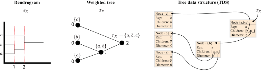
Figure 8: Tree structure of dendrograms. The leftmost figure represents the dendrogram $\theta_{X}$ of a three-point ultrametric space $X$. The middle figure represents the weighted rooted tree $T_{X}$ associated to $X$. The numbers beside the nodes represent the weight values given by $w_{X}$. Note that the tree structure of $T_{X}$ is inherited directly from the tree structure of $\theta_{X}$. The rightmost figure shows the TDS associated to $T_{X}$.

Remark 60.

It is obvious that the set of singletons $\{\{x\}\in V_{X}:\,x\in X\}$ coincides with the set of leaves of $T_{X}$. Since for every rooted tree $\#\mathrm{vertices}=O(\#\mathrm{leaves})$ (indeed, $\#\mathrm{leaves}\leq\#\mathrm{vertices}\leq 2\#\mathrm{leaves}$), we have that $\#V_{X}=O(n)$ where $n\coloneqq\#X$. Moreover, since $\#E_{X}=\#V_{X}-1=O(V_{X})$, we have that $\#E_{X}=O(n)$ as well.

Proposition 61 ([13, Theorem 1.10]).

For any two finite ultrametric spaces $X$ and $Y$, let $T_{X}$ and $T_{Y}$ denote their corresponding weighted rooted trees. Then, $X$ is isometric to $Y$ iff $T_{X}$ is isomorphic to $T_{Y}$.

Remark 62 (Relation to merge trees).

For the precise definition of merge trees, see for example [32]. Let $X$ be a finite ultrametric space and let $T_{X}$ be its associated weighted rooted tree. We first transform $T_{X}$ into a topological/metric tree by replacing each edge $\{B,B^{\prime}\}$ with an interval with length $|\mathrm{diam}(B)-\mathrm{diam}(B^{\prime})|$. We then attach to the root $r_{X}$ the half line $[0,\infty)$ to obtain the topological space $M_{X}$. We then define the height function $h_{X}:M_{X}\rightarrow\mathbb{R}$ as follows:

1. $h_{X}(B)=w_{X}(B)=\mathrm{diam}(B)$ for each $B\in V_{X}$;

2. for each edge, inside its corresponding interval, $h_{X}$ is defined as the linear interpolation between the function values at the end points;

3. for $t$ on the half line $[0,\infty)$, $h_{X}(t)\coloneqq h_{X}(r_{X})+t$.

In this way, each finite ultrametric space $X$ canonically induces the merge tree $\left(M_{X},h_{X}\right)$.

Remark 63 (Detailed comparison between $\gamma_{\varepsilon}(X)$ and $\tau_{\varepsilon}(M_{X})$).

Recall that for $\varepsilon\geq 0$, the $\varepsilon$-degree bound $\tau_{\varepsilon}(M_{X})$ of a merge tree $M_{X}$ is the maximum over all closed $\varepsilon$ balls the sum of degrees of all vertices inside the ball (cf. Remark 40). By Remark 62, each finite ultrametric space $X$ canonically induces the merge tree $(M_{X},h_{X})$. Then, we call $\tau_{\varepsilon}(X)\coloneqq\tau_{\varepsilon}(M_{X})$ the $\varepsilon$-degree bound of the ultrametric space $X$. It is easy to see that for any ultrametric space $X$, we have that

$$\gamma_{\varepsilon}(X)\leq\tau_{\varepsilon}(X)\leq 2\gamma_{\varepsilon}(X).$$

See Figure 9 for an illustration and a sketch of the proof of this fact. In particular, this implies that $X\in\mathcal{U}_{2}(\frac{\varepsilon}{2},\gamma)$ for all $\gamma\geq\tau_{\varepsilon}(X)$.

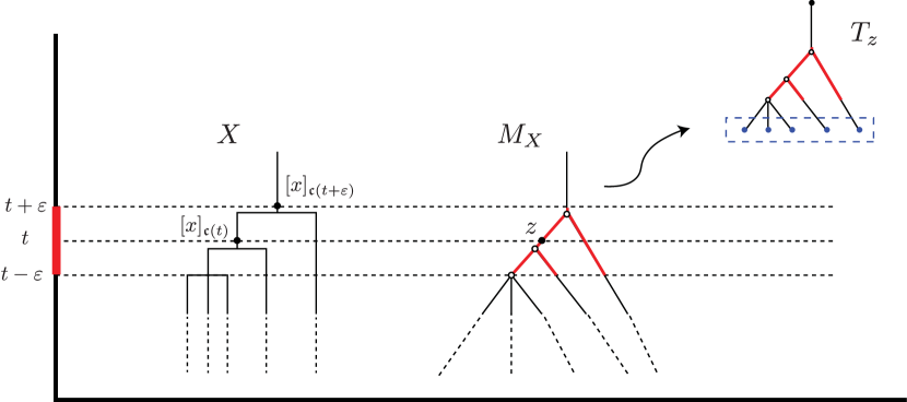
Figure 9: Illustration of Remark 63. In this figure, we draw part of the dendrogram of an ultrametric space $X$ and its corresponding merge tree $M_{X}$. Pick any $z\in M_{X}$ with height $t$. Then, $z$ corresponds to $[x]_{\mathfrak{c}(t)}$ for some point $x\in X$ (cf. Remark 62). Consider the closed ball $B_{\varepsilon}^{M_{X}}(z)\subseteq M_{X}$ highlighted in red in the figure. Considering a small closed neighborhood of the highlighted part in $M_{X}$, we obtain the rooted tree $T_{z}$ in the top right corner of the figure. It is obvious that the number of leaves of $T_{z}$ inside the dotted box equals $\gamma_{\varepsilon}(x,t+\varepsilon)\coloneqq\#\left\{{[x^{\prime}]_{\mathfrak{o}\left(t-\varepsilon\right)}}:\,x^{\prime}\in[x]_{\mathfrak{c}\left(t+\varepsilon\right)}\right\}$. On the other hand, the sum of degrees of vertices of the tree $M_{X}$ contained in the ball $B_{\varepsilon}^{M_{X}}(z)$, denoted by $\tau_{\varepsilon}(z)$, equals the number of edges in $T_{z}$. Therefore, by the standard relationship between the number of leaves and the number of edges in a rooted tree, we have that $\gamma_{\varepsilon}(x,t+\varepsilon)\leq\tau_{\varepsilon}(z)\leq 2\,\gamma_{\varepsilon}(x,t+\varepsilon)$. From this observation, we conclude that $\gamma_{\varepsilon}(X)\leq\tau_{\varepsilon}(X)\leq 2\,\gamma_{\varepsilon}(X).$

A.2 Data structure for ultrametric spaces and algorithms for fundamental operations

Given a finite ultrametric space $(X,u_{X})$, let $T_{X}$ be its corresponding weighted rooted tree as described in Definition 59. We utilize a special self-referential tree structure to represent $T_{X}$; for a description of self-referential tree data structures, we refer readers to [22, Chapter 6.5]. In order to represent vertices of $T_{X}$, we design a special class Node with three fields: Representative, Diameter and Children. Recall that each vertex of $T_{X}$ represents a closed ball of $X$. Then, for each vertex/ball $B\in V_{X}$, its corresponding Node object, which will still be denoted by $B$, contains the following fields:

1. Representative: an element $x\in B$;

2. Diameter: the diameter of $B$;

3. Children: a list of pointers to all Node objects representing the children of $B$ in $T_{X}$.

In what follows, we will sometimes call a Node object simply a node and we will for instance write $B.\texttt{Diameter}$ to extract the diameter value of a node $B$.

Now, for a given ultrametric space $X$, the tree data structure (TDS) which we will use to represent $T_{X}$ consists of a collection of nodes stored in memory, one for each vertex $B\in V_{X}$. This TDS is held by a Node pointer referencing the node representing the root $r_{X}=X$. We call this pointer (to a Node object) the root pointer of the TDS. The role of the root pointer of a TDS is analogous to the role of the head pointer of a linked list. See Figure 8 for an illustration.

Note. In the sequel, we will overload the symbol $T_{X}$ and will use it to denote both the weighted rooted tree corresponding to $X$ and to also represent its associated TDS (both in the sense of its root pointer and in the sense of the collection of its nodes). The symbol $B$ for representing any ball $B\in V_{X}$ is also overloaded to represent its corresponding Node object in $T_{X}$. In all our algorithms, every ultrametric space is understood as a Node object.

Remark 64 (Relationship with the distance matrix data structure).

Starting from the root node $r_{X}$ of $T_{X}$, one can progressively trace all nodes in $T_{X}$ to completely reconstruct the distance matrix of the ultrametric space $X$. It is clear that the reconstruction process takes time at most $O(n^{2})$ where $n\coloneqq\#X$. Conversely, given the distance matrix of $X$, one can construct the TDS $T_{X}$ in the same time complexity $O(n^{2})$ (one can use for example the single-linkage algorithm [33] to first obtain the dendrogram induced by the distance matrix (see Figure 8)). If the ultrametric spaces are given in terms of distance matrices, we first need to convert them into TDSs before applying the algorithms described in this paper. The time complexity $O(n^{2})$ due to this preprocessing is not counted when analyzing our algorithms.

Remark 65 (Subtree rooted at a ball).

Given the TDS $T_{X}$ associated to the ultrametric space $X$, it is easy to induce a TDS $T_{B}$ for each closed ball $B\in V_{X}$ (which is itself an ultrametric space). Such $T_{B}$ consists of all descendant nodes of $B$ in $T_{X}$ and is held by a pointer to $B$, i.e., $*(T_{B})=B$. Here $*p$ denotes the datum referenced by a pointer $p$.

Remark 66 (Finding parent nodes).

Given any non-root node $B$ in $T_{X}$, we let $\texttt{Parent}(B,T_{X})$ denote its parent node in $T_{X}$. To actually find the node $\texttt{Parent}(B,T_{X})$ given the node $B$, one can start from the root node $r_{X}$ and recursively search $T_{X}$ for the parent of $B$. Such a search process takes at most time $O(\#T_{X})=O(n)$ where $n\coloneqq\#X$.

One major advantage of adopting the above-mentioned TDS is that it allows us to efficiently implement certain fundamental operations on ultrametric spaces. For example, it allows to efficiently obtain the spectrum of an ultrametric space:

Lemma 67.

Given an ultrametric space $X$, determining and sorting $\mathrm{spec}(X)$ can be done in time $O(n\log(n))$ where $n\coloneqq\#X$.

Proof.

Note that, by Lemma 58, we only need to inspect each node in $T_{X}$ which takes time $O(n)$. Since $\#\mathrm{spec}(X)=O(n)$ (cf. Proposition 7), the sorting process takes time $O(n\log(n))$. ∎

Next, we introduce algorithms for other three fundamental operations on ultrametric spaces.

Closed quotient

In Algorithm 6 we introduce a recursive algorithm for the $t$-closed quotient operation. In the algorithm, the notation $\leftarrow$ represents variable assignment and the notation $\&Z$ denotes the memory address of the variable $Z$. In line 6 of the algorithm, the one point tree data structure consists of a single node such that $\texttt{Diameter}=0$ and Children is an empty list. Note that in the worst-case scenario, Algorithm 6 inspects all nodes of $T_{X}$ during the recursion process. At the recursion call with input $(B,t)$ where $B$ is a node of $T_{X}$, the main computational cost lies in line 1 for copying the Node object $B$ (in the place of $X$). If we let $k_{B}\coloneqq\mathrm{length}(B.\texttt{Children})$, it then costs time $O(k_{B})$ to copy $B$ and it takes at most time $O(k_{B})$ to update $B.\texttt{Children}$ according to the for-loop in line 2. Therefore, the total time complexity of Algorithm 6 is bounded above by $\sum_{B\in V_{X}}O(k_{B})$. By Lemma 56 and Remark 60, we have that

$$\sum_{B\in V_{X}}O(k_{B})=O(V_{X})=O(n),$$

where $n\coloneqq\#X$. Therefore, the time complexity of Algorithm 6 is bounded above by $O(n)$.

Algorithm 6 $\mathbf{ClosedQuotient}(X,t)$

1:  $Y\leftarrow X$ 

2:  for Each $p\in Y.\texttt{Children}$ do

3:     if $*p.\texttt{Diameter}>t$ then

4:        $p\leftarrow\&\mathbf{ClosedQuotient}(*p,t)$

5:     else

6:        $Z\leftarrow$ the one point tree with the same representative in $*p$

7:        $p\leftarrow\&Z$

8:     end if

9:  end for

10:  return  $Y$

Open partition

In Algorithm 7 we give pseudocode for constructing the $t$-open partition of an ultrametric space. In order to implement the ‘append’ operation (appearing in line 3 and line 6) in constant time, we use a doubly linked list $P$ to represent the open partition. Algorithm 7 will recursively inspect all nodes corresponding to balls in $X_{\mathfrak{o}(t)}$ as well as all of their ancestor nodes. For each inspected node $B$ in $T_{X}$, if we let $k_{B}\coloneqq\mathrm{length}(B.\texttt{Children})$, it then takes time $O(k_{B})$ to update the list $P$. Then, following a similar argument as in the complexity analysis of Algorithm 6, if we let $k$ be the cardinality of $P$ (i.e., $k=\#X_{\mathfrak{o}(t)}$), then Algorithm 7 will inspect at most $O(k)$ nodes in $T_{X}$ and thus it generates $P$ in at most $O(k)$ steps.

Algorithm 7 $\mathbf{OpenPartition}(X,t)$

1:  $P=[\,]$

2:  if $X.\texttt{Diameter}<t$ then

3:     $P.\mathrm{append}(\&X)$

4:  else

5:     for Each $p_{i}\in X.\texttt{Children}$ do

6:        $P.\mathrm{append}(\mathbf{OpenPartition}(*p_{i},t))$

7:     end for

8:  end if

9:  return  $P$

Isometry between ultrametric spaces

By Proposition 61, two ultrametric spaces $X$ and $Y$ are isometric iff their corresponding weighted rooted trees $T_{X}$ and $T_{Y}$ are isomorphic. By adapting the algorithm in [3, Example 3.2], determining isomorphism between rooted trees can be done in time $O(\#\mathrm{vertices})$; see also [3, Theorem 3.3] (and its corollary). Then, by Remark 60, we have the following result:

Lemma 68.

We can determine whether $X$ and $Y$ are isometric in $O(n)$ time.

A.3 Subspace tree data structure and union of non-intersecting subspaces

In this section, we explain how to utilize the TDS described in the previous section to efficiently perform the union operation (under the conditions specified by Equation (14) below).

First of all, we introduce a TDS for representing subspaces of a given ultrametric space $X$. We assume that the distance matrix $u_{X}$ is available and assume that a TDS $T_{X}$ representing $X$ has already been computed.

Definition 69 (Subspace tree data structure).

For any non-empty subspace $U\subseteq X$, we say that a tree data structure $T_{U}$ representing the ultrametric space $(U,u_{X}|_{U\times U})$ is a subspace tree data structure subordinate to $T_{X}$, if each vertex (i.e., each ball) in $V_{U}\cap V_{X}$ is represented by a Node object belonging to the tree data structure $T_{X}$.

Remark 70 (Construction of subspace TDSs).

For any node $B\in T_{X}$ (which represents a ball in $X$), the TDS $T_{B}$ described in Remark 65 is obviously a subspace TDS subordinate to $T_{X}$ representing the subspace $B$. However, for an arbitrary subset $U$ the situation is different from the case of a ball. First, it is easy to verify that any such $U$ can be written as a union of non-intersecting balls $\{B_{i}\}_{i=1}^{k}$ satisfying the condition in Equation (14) (see also Lemma 71 below). Then, a subspace TDS representing $U$ subordinate to $X$ can be constructed by applying the union process which we describe below to the set of balls $\{B_{i}\}_{i=1}^{k}$.

Consider a set of non-empty and non-intersecting subspaces $\{U_{1},\ldots,U_{k}\}$ of a given ultrametric space $X$ such that for any distinct $i,j=1,\ldots,k$, we have

$$\min_{x_{i}\in U_{i},x_{j}\in U_{j}}u_{X}(x_{i},x_{j})>\max(\mathrm{diam}(U_{i}),\mathrm{diam}(U_{j})).$$ (14)

This condition is compatible with the sets obtained by taking a slice of the dendrogram $\theta_{X}$, which is in turn equivalent to considering open/closed equivalence classes of ultrametric spaces (see the discussion below Definition 13). We assume that each $U_{i}$ is represented by a subspace TDS $T_{U_{i}}$ subordinate to $T_{X}$.

Now given the above data, we describe how to construct a subspace TDS $T_{U}$ subordinate to $T_{X}$ representing the union $U\coloneqq\cup_{i=1}^{k}U_{i}$. The whole process is organized through the following three steps.

(i@) Constructing a TDS induced by representatives

For each $i=1,\ldots,k$ let $x_{i}$ be the representative of $U_{i}$ as given in the TDS $T_{U_{i}}$ and let $X_{k}\coloneqq\{x_{1},\ldots,x_{k}\}$. We first consider the ultrametric $u_{X_{k}}\coloneqq u_{X}|_{X_{k}\times X_{k}}$ on $X_{k}$ induced by the restriction of $u_{X}$ to $X_{k}\times X_{k}$. Then, we construct a new TDS $T_{X_{k}}$ to represent $(X_{k},u_{X_{k}})$ (cf. Remark 64). This construction is possible due to the fact that $(X_{k},u_{X_{k}})$ is itself an ultrametric space.

It takes time at most $O(k^{2})$ to both construct the metric $u_{X_{k}}$ and create the new TDS $T_{X_{k}}$ (cf. Remark 64).

(ii@) Constructing the preliminary union of $U_{i}$s

Recall that up to this point, we have at our disposal the following TDSs: $T_{U_{1}},\ldots,T_{U_{k}}$, and $T_{X_{k}}$. Based on these data, we progressively modify leaf nodes of $T_{X_{k}}$ and utilize $T_{U_{1}},\ldots,T_{U_{k}}$ to find a TDS representation for the union $U$. For pedagogical reasons, we refer to the outcome TDS as $\tilde{T}_{U}$. $\tilde{T}_{U}$ may not be subordinate to $T_{X}$, and we thus name it the preliminary union of $U_{i}$s. The modification process can be summarized as simply replacing each leaf node in $T_{X_{k}}$ with the root node of certain $T_{U_{i}}$ as shown in Figure 10. More precisely, we traverse all nodes $B$ in $T_{X_{k}}$ and, if for such a node $B$ there exists an index $i_{0}$ such that $*(B.\texttt{Children}(i_{0})).\texttt{Diameter}=0$ (which means $B$ is the parent of a leaf node), then we let $j_{0}$ be the index such that $*(B.\texttt{Children}(i_{0})).\texttt{Representative}=x_{j_{0}}\in X_{k}$, and modify $B$ by assigning $B.\texttt{Children}(i_{0})=T_{U_{j_{0}}}$ (and of course we free the memory used for storing the original node $*(B.\texttt{Children}(i_{0}))$).

Figure 10: Illustration of the process for producing the preliminary union $\tilde{T}_{U}$.

For the modification process described above, we need to modify at most $O(k)$ pointers, and for each such pointer it takes time $O(k)$ to search for $U_{j_{0}}$ with the desired representative as described above. So, the time needed for constructing the preliminary union $\tilde{T}_{U}$ is at most $O(k^{2})$.

(iii@) Taming process for $\tilde{T}_{U}$

The TDS $\tilde{T}_{U}$ may not be a subspace TDS subordinate to $T_{X}$, i.e., $\tilde{T}_{U}$ may contain Node objects representing balls in $V_{X}$ which do not belong to the TDS $T_{X}$. We will thus further tame $\tilde{T}_{U}$ so that the outcome TDS is subordinate to $T_{X}$. For pedagogical reasons, we use the symbol $T_{U}$ (which is our final TDS representation for $U$) to refer to the tamed $\tilde{T}_{U}$.

To accomplish this, we first create an array $\mathrm{L}$ consisting of pointers to all nodes in $\tilde{T}_{U}\backslash\cup_{i=1}^{k}T_{U_{i}}$, i.e., all modified nodes from $T_{X_{k}}$. We sort $\mathrm{L}$ according to increasing Diameter values of the nodes referenced by its pointers. There are $O(k)$ such nodes and thus building and sorting $\mathrm{L}$ takes time $O(k\log(k))$. Let $\ell\coloneqq\mathrm{length}(\mathrm{L})=O(k)$. For each $i=1,\ldots,\ell$, we compare $*(\mathrm{L}(i))$ with each node in $T_{X}$ as described next. If for some $B\in T_{X}$, the sets $B.\texttt{Children}$ and $*(\mathrm{L}(i)).\texttt{Children}$ agree, we then replace the node $*(\mathrm{L}(i))$ in $\tilde{T}_{U}$ with $B$. There are two cases which can arise during this replacement:

1. if $*(\mathrm{L}(i))$ is not the root node of $*(\tilde{T}_{U})$, we find the parent node of $*(\mathrm{L}(i))$ (cf. Remark 66) in $\tilde{T}_{U}$ and let $i_{0}$ be the index such that $\texttt{Parent}\left(*(\mathrm{L}(i)),\tilde{T}_{U}\right).\texttt{Children}(i_{0})=\mathrm{L}(i)$. Then, we replace $\texttt{Parent}\left(*(\mathrm{L}(i)),\tilde{T}_{U}\right).\texttt{Children}(i_{0})$ with a pointer to $B\in T_{X}$;

2. otherwise if $*(\mathrm{L}(i))$ is the root node $*(\tilde{T}_{U})$, we free the memory used for storing $*(\tilde{T}_{U})$, and then assign $\tilde{T}_{U}=\&B$.

For each $i=1,\ldots,\ell$ let $k_{i}\coloneqq\mathrm{length}(*(\mathrm{L}(i)).\texttt{Children})$. Determining whether $B.\texttt{Children}=*(\mathrm{L}(i)).\texttt{Children}$ takes time $O(k_{i})$. Therefore, the time complexity of the replacement process mentioned above can be bounded as follows:

$$\sum_{i=1}^{\ell}O(\#T_{X})\times k_{i}=\sum_{i=1}^{\ell}O(nk_{i})=O\left(n\sum_{i=1}^{\ell}k_{i}\right)=O(nk),$$

where $n\coloneqq\#X$ (we used Lemma 56 in the rightmost equality). The time incurred when finding and accessing the parent node of a given node in $\mathrm{L}$ is at most $O(k)$ (cf. Remark 66). So the total time required for taming $\tilde{T}_{U}$ is at most $O(nk)$.

Therefore by following steps (i@), (ii@) and (iii@), the total time complexity of the union operation can be bounded by $O(k^{2})+O(nk)=O(nk)$.

A.4 Implementation details for Algorithm 4

In this section, we provide details for one possible implementation of Algorithm 4.

A.4.1 Preprocessing

To achieve an actual implementation of Algorithm 4, some preprocessing is needed in order to construct the arrays $\mathrm{LX}^{(\varepsilon)}$ and $\mathrm{LY}$ defined in Section 5.2.3. Here, for completeness we describe one possible implementation of these preprocessing steps. We first construct subspace TDSs for subspaces in $\mathrm{LX}^{(\varepsilon)}$ and $\mathrm{LY}$. We then construct arrays $\mathrm{pLX}^{(\varepsilon)}$ and $\mathrm{pLY}$ of Node pointers referencing subspaces in $\mathrm{LX}^{(\varepsilon)}$ and $\mathrm{LY}$, respectively. For this purpose, we augment the class Node by incorporating an integer field called Order and a Boolean field called IsBall. For each node $B$ in $T_{X}$, Order is initially set to $-1$ and IsBall is set to True. We initialize nodes in $T_{Y}$ in the same way.

Construction of $\mathrm{pLY}$

Given the TDS $T_{Y}$, we first create an array $\mathrm{pLY}$ containing pointers to all nodes in $T_{Y}$. Then, we sort $\mathrm{pLY}$ according to increasing Diameter values of the Node objects referenced by its pointers. This finalizes constructing the array $\mathrm{pLY}$. For each $i=1,\ldots,\#\mathrm{pLY}$, we set $*(\mathrm{pLY}(i)).\texttt{Order}=i$. In this way, each element in $T_{Y}$ is such that its field Order is different from $-1$.

By Lemma 88, $\#T_{Y}=\#V_{Y}=O(n)$. So building and sorting the list $\mathrm{pLY}$ can be done in time $O(n\log(n))$. The above process for setting $B^{Y}.\texttt{Order}$ for all $B^{Y}\in\mathrm{pLY}$ can be done in time $O(n)$.

Construction of $\mathrm{pLX}^{(\varepsilon)}$

Unlike the case of $\mathrm{LY}$, the array $\mathrm{LX}^{(\varepsilon)}$ can contain subspaces not belonging to $V_{X}$. In order to construct $\mathrm{pLX}^{(\varepsilon)}$, we follow the three steps that we describe next:

1. Create subspace TDSs subordinate to $T_{X}$ for representing each of the subspaces in $\mathrm{LX}^{(\varepsilon)}\backslash\mathrm{LX}$;

2. Create a list $\mathrm{pLX}^{(\varepsilon)}$ of pointers referencing the root nodes representing each of the subspaces in $\mathrm{LX}^{(\varepsilon)}$.

3. Transform the list $\mathrm{pLX}^{(\varepsilon)}$ into an array (still denoted by $\mathrm{pLX}^{(\varepsilon)}$). In this way, the random access time to elements in $\mathrm{pLX}^{(\varepsilon)}$ is $O(1)$.

Whereas the third step is clear, we will provide a detailed description for the first and second steps. In fact, these two steps are accomplished at the same time: We first construct $\mathrm{pLX}$ via a process analogous to the one used above for constructing $\mathrm{pLY}$. This step can be done in time $O(n\log(n))$. Then, we follow two substeps: (a) for each $B^{X}\in\mathrm{LX}$, we will first construct subspace TDSs subordinate to $T_{X}$ for all subspaces in $B^{X}_{(\varepsilon)}\backslash\{B_{X}\}$; we then construct the list $\mathrm{p}B^{X}_{(\varepsilon)}$ of pointers referencing all subspaces in $B^{X}_{(\varepsilon)}$; (b) we will use these constructions from (a) for all $B^{X}$ to complete step 1 and step 2. Below, we describe substep (a) and substep (b) in detail.

(a) Constructions regarding a single $B^{X}$

We set $\mathrm{p}B^{X}_{(\varepsilon)}$ to be an empty list. Applying $\mathbf{OpenPartition}$ (Algorithm 7) to $B^{X}$ we obtain the open partition $B^{X}_{\mathfrak{o}\left(\rho_{\varepsilon}\left(B^{X}\right)\right)}=\left\{B_{i}\right\}_{i=1}^{N_{B^{X}}}$. By the SGC, $N_{B^{X}}\leq\gamma$ so that the open partition process takes time at most $O(\gamma)$. For each non-empty index set $I\subseteq[N_{B^{X}}]$ (there are $O(2^{\gamma})$ such $I$s), we apply the union operation (described in Appendix A.3) to obtain the TDS $T_{U_{I}}$ for the union $U_{I}\coloneqq\cup_{i\in I}B_{i}$ which takes time at most $O(n\times\#I)=O(n\gamma)$. For the new nodes thus created, i.e., for nodes $U$ in $T_{U_{I}}\backslash T_{X}$, we set $U.\texttt{IsBall}=\texttt{False}$ and set $U.\texttt{Order}=-1$. If $U_{I}.\texttt{Diameter}=B^{X}.\texttt{Diameter}$, we first set $U_{I}.\texttt{Order}=B^{X}.\texttt{Order}$ and then update $\mathrm{p}B^{X}_{(\varepsilon)}$ by appending $T_{U_{I}}$ (which is a pointer to the node $U_{I}$) to it. Otherwise, we delete all nodes in $T_{U_{I}}\backslash T_{X}$.

In summary, the time complexity for both constructing subspace TDSs subordinate to $T_{X}$ for all elements in $B^{X}_{(\varepsilon)}\backslash\{B_{X}\}$ and constructing the list $\mathrm{p}B^{X}_{(\varepsilon)}$ is bounded by $O(n2^{\gamma}\gamma^{2})$.

(b) Completing step 1 and step 2

Finally, we apply the constructions described above to all $B^{X}\in\mathrm{LX}$ and assemble the corresponding outputs to complete step 1 and step 2 concurrently. More specifically, we first sort $\mathrm{LX}$ according to increasing values of Order. Then, we apply the above constructions over all $B^{X}\in\mathrm{LX}$ with respect to this order. After this, subspace TDSs for all elements in $\mathrm{LX}^{(\varepsilon)}\backslash\mathrm{LX}$ have been constructed and stored in memory. Finally, we merge all the resulting lists $\mathrm{p}B^{X}_{(\varepsilon)}$s together to obtain the list $\mathrm{pLX}^{(\varepsilon)}$. Since $\#\mathrm{LX}=O(n)$ and since for each $B^{X}$, $\mathrm{length}(\mathrm{p}B^{X}_{(\varepsilon)})=O(2^{\gamma})$, the time needed for constructing subspace TDSs for elements in $\mathrm{LX}^{(\varepsilon)}\backslash\mathrm{LX}$ is bounded by $O(n^{2}2^{\gamma}\gamma^{2})$, and the merging process takes time at most $O(n2^{\gamma})$ (the complexity can be reduced to $O(n)$ if each $\mathrm{p}B^{X}_{(\varepsilon)}$ is represented by a doubly linked list).

Therefore, step 1 and step 2 together can be accomplished in time

$$O\big{(}n\log(n)+n^{2}2^{\gamma}\gamma^{2}+n2^{\gamma}\big{)}=O\big{(}n^{2}\log(n)2^{\gamma}\gamma^{2}\big{)}.$$

Since $\#\mathrm{pLX}^{(\varepsilon)}=O(n2^{\gamma})$, the time for transforming $\mathrm{pLX}^{(\varepsilon)}$ into an array is bounded by $O(n2^{\gamma})$. So, the total time complexity for building the array $\mathrm{pLX}^{(\varepsilon)}$ is at most $O\big{(}n^{2}\log(n)2^{\gamma}\gamma^{2}\big{)}$.

Data structure for storing and accessing indices of elements in $\mathrm{LX}^{(\varepsilon)}$

Given any $U^{X}\in\mathrm{LX}^{(\varepsilon)}$, there exists a unique integer $\mathrm{ind}$ such that $U^{X}=*(\mathrm{pLX}^{(\varepsilon)}(\mathrm{ind}))$ and we refer to $\mathrm{ind}$ as the index of $U^{X}$ in $\mathrm{LX}^{(\varepsilon)}$. Now, given any $U^{X}$ in the form of a subspace TDS subordinate to $T_{X}$, in order to access the index of $U^{X}$ in $\mathrm{LX}^{(\varepsilon)}$ efficiently, we construct a $\underbrace{(1+\#V_{X})\times\cdots\times(1+\#V_{X})}_{\gamma\text{ terms}}$ dimensional multi-array $\mathrm{INDX}$ for storing all such indices. Each dimension of $\mathrm{INDX}$ is indexed by integers in the range $\{-1\}\cup\{1,\ldots,\#V_{X}\}$. The following lemma gives rise to our strategy for indexing this multi-array.

Lemma 71.

For any subset $U^{X}\subseteq X$, there is a unique maximal set of non-intersecting closed balls $\{B_{1},\ldots,B_{k}\}\subseteq V_{X}$ such that $U^{X}=\cup_{i=1}^{k}B_{i}$. Here ‘maximal’ means that if there exists another set of non-intersecting closed balls $\{B_{1}^{\prime},\ldots,B_{l}^{\prime}\}\subseteq V_{X}$ such that $U^{X}=\cup_{i=1}^{l}B_{i}^{\prime}$, then for each $i=1,\ldots,l$, there exists some $j=1,\ldots,k$ such that $B_{i}^{\prime}\subseteq B_{j}$. We call the unique maximal set $\{B_{1},\ldots,B_{k}\}\subseteq V_{X}$ the ball decomposition of $U^{X}$.

Now, given $U^{X}\in\mathrm{LX}^{(\varepsilon)}$, let $\mathrm{ind}$ denote its index in $\mathrm{LX}^{(\varepsilon)}$. Let $\{B_{1},\ldots,B_{k}\}$ be the ball decomposition of $U^{X}$ whose elements are labeled such that

$$B_{1}.\texttt{Order}<\cdots<B_{k}.\texttt{Order}.$$

We then store $\mathrm{ind}$, the index of $U^{X}$, in $\mathrm{INDX}$ as follows

$$\mathrm{INDX}(B_{1}.\texttt{Order},B_{2}.\texttt{Order},\ldots,B_{k}.\texttt{Order},\underbrace{-1,\ldots,-1)}_{\gamma-k\text{ terms}}=\mathrm{ind}.$$

Computation of the ball decomposition

Given $U^{X}\in\mathrm{LX}^{(\varepsilon)}$, we proceed to compute its ball decomposition as follows. If $U^{X}.\texttt{Order}\neq-1$, then $U^{X}\in\mathrm{LX}$, i.e., $U^{X}$ already represents a ball in $X$. In this case, $\{U^{X}\}$ is the ball decomposition of $U^{X}$. Otherwise, we traverse all nodes of $T_{U^{X}}$ to create the list $\mathrm{p}U^{X}$ consisting of pointers to all nodes $\{B_{1},\ldots,B_{k}\}\subseteq T_{U^{X}}$ such that: for each $i=1,\ldots,k$, $B_{i}.\texttt{IsBall}=\texttt{True}$ but the parent node of $B_{i}$ satisfies $\texttt{Parent}\left(B_{i},T_{U^{X}}\right).\texttt{IsBall}=\texttt{False}$. Then, $\{B_{1},\ldots,B_{k}\}$ is the desired ball decomposition of $U^{X}$.

The computation of the ball decomposition of $U^{X}\in\mathrm{LX}^{(\varepsilon)}$ described above can be done in time $O(\gamma\log(\gamma))$ (including the sorting time). Therefore, the total time complexity for storing the indices of all $U^{X}\in\mathrm{LX}^{(\varepsilon)}$ into $\mathrm{INDX}$ is bounded by $O(n2^{\gamma}\gamma\log(\gamma))$ and the time needed for finding the index of $U^{X}$ into $\mathrm{LX}^{(\varepsilon)}$ is bounded by $O(\gamma\log(\gamma))$. We remark that the space complexity of the multi-array $\mathrm{INDX}$ is $O(n^{\gamma})$. The actual size of $\mathrm{LX}^{(\varepsilon)}$ is however $O(n2^{\gamma})$. To reduce the space complexity, one could consider a sparse multi-array data structure or binary search trees.

A.4.2 A refined union operation via an improved taming process

In line 16 of Algorithm 4 we need to construct the union space $U_{\Psi^{-1}(j)}^{X}\coloneqq\cup_{i\in\Psi^{-1}(j)}U_{i}^{X}$ where all $U_{i}^{X}$s are subspaces of $U^{X}$. By the SGC, $\#\Psi^{-1}(j)=O(\gamma)$. Therefore, by results in Section A.3, it takes time $O(n\gamma)$ to construct a subspace TDS (subordinate to $T_{X}$) for representing $U_{\Psi^{-1}(j)}^{X}$ given the subspace TDSs (subordinate to $T_{X}$) for $U_{i}^{X}$s.

Recall from Appendix A.3 that the union operation consists of three steps where the final step, i.e., the taming process, has the leading time complexity. In this section, we provide a refined union operation via an improved taming process for constructing $U_{\Psi^{-1}(j)}^{X}$ such that the time complexity of this refined union operation is thus reduced to $O(\gamma^{2})$. In the sequel, we use the shorthand $U\coloneqq U_{\Psi^{-1}(j)}^{X}$ and also let $k\coloneqq\#\Psi^{-1}(j)=O(\gamma)$.

Note that in Appendix A.3, the taming process for the preliminary union $\tilde{T}_{U}$ requires pairwise comparisons between all nodes in $\tilde{T}_{U}\backslash\cup_{i=1}^{k}T_{U_{i}}$ and all nodes in $T_{X}$. The fact that $\#T_{X}=O(n)$ explains the $n$ factor in the time complexity bound $O(nk)$ for the taming process. However, to tame $\tilde{T}_{U}$, we only need to compare every node in $\tilde{T}_{U}\backslash\cup_{i=1}^{k}T_{U_{i}}$ with a certain subset of nodes in $T_{X}$. We obtain the improved taming process for $\tilde{T}_{U}$ by restricting the pairwise comparisons in this way and by keeping the rest of the taming process unchanged.

Now, we explain how to restrict the pairwise comparison. Let $i_{0}\coloneqq U^{X}.\texttt{Order}$ and let $B^{X}\coloneqq\mathrm{LX}(i_{0})$. Since $U^{X}\in\mathrm{LX}^{(\varepsilon)}$, we have that $U^{X}\in B^{X}_{(\varepsilon)}$, i.e., the set of $\varepsilon$-maximal unions of closed balls in $B^{X}$ (cf. Section 5.2.3). Starting from the node $B^{X}$, we traverse all of its descendants $B$ in order to identify all those for which $B.\texttt{Diameter}\geq B^{X}.\texttt{Diameter}-2\varepsilon$. We let $\mathrm{L}B^{X}$ denote the set of all such descendants. Then, in the improved taming process of $\tilde{T}_{U}$, we only compare all nodes in $\tilde{T}_{U}\backslash\cup_{i=1}^{k}T_{U_{i}}$ with all nodes in $\mathrm{L}B^{X}$.

By the SGC, $\#\mathrm{L}B^{X}=O(\gamma)$ and thus the time complexity of the improved taming process described above is at most $O(\gamma k)=O(\gamma^{2})$. Therefore, constructing $T_{U}$ via this taming process has cost at most $O(\gamma^{2})$.

Appendix B Extension of $u_{\mathrm{GH}}$ to ultra-dissimilarity spaces

In this section, we will consider the collection $\mathcal{U}^{\mathrm{dis}}$ of finite ultra-dissimilarity spaces, which are generalizations of ultrametric spaces (see also [42] for a more general notion called ultra-network).

Definition 72 (Ultra-dissimilarity space).

An ultra-dissimilarity space is any pair $(X,u_{X})$ where $X$ is a finite set and $u_{X}:X\times X\rightarrow\mathbb{R}_{\geq 0}$ satisfies, for all $x,x^{\prime},x^{\prime\prime}\in X$:

1. Symmetry: $u_{X}(x,x^{\prime})=u_{X}(x^{\prime},x)$,

2. Strong triangle inequality: $u_{X}(x,x^{\prime\prime})\leq\max\left(u_{X}(x,x^{\prime}),u_{X}(x^{\prime},x^{\prime\prime})\right),$

3. Definiteness: $\max\left(u_{X}(x,x),u_{X}(x^{\prime},x^{\prime})\right)\leq u_{X}(x,x^{\prime})$, and the equality takes place if and only if $x=x^{\prime}$.

We refer to $u_{X}$ as the ultra-dissimilarity on $X$. It is obvious that any finite ultrametric space is an ultra-dissimilarity space. Then, $\mathcal{U}^{\mathrm{fin}}\subseteq\mathcal{U}^{\mathrm{dis}}$, where $\mathcal{U}^{\mathrm{fin}}$ denotes the collection of finite ultrametric spaces.

We say two ultra-dissimilarity spaces $(X,u_{X})$ and $(Y,u_{Y})$ are isometric if there exists a bijective function $f:X\rightarrow Y$ such that for any $x,x^{\prime}\in X$

$$u_{Y}(f(x),f(x^{\prime}))=u_{X}(x,x^{\prime}).$$

Such an $f$ is called an isometry.

Remark 73 (Informal interpretation).

For each $x\in X$, the value $u_{X}(x,x)$ is regarded as the ‘birth time’ of the point $x$; when $u_{X}$ is an actual ultrametric on $X$, all points are born at time $0$. The value $u_{X}(x,x^{\prime})$ for different points $x$ and $x^{\prime}$ encodes the time when the two points ‘merge’. Note that then condition (3) above can be informally interpreted as encoding the property that two points cannot merge before their respective birth times, and that if they merge at the same time they are born, then they are actually the same point.

Given two ultra-dissimilarity spaces $X$ and $Y$ and any correspondence $R$ between them, without any obstacle, we define $\mathrm{dis}_{\infty}(R)$ in exactly the same way by Equation (8), i.e.,

$$\mathrm{dis}_{\infty}(R)\coloneqq\sup_{(x,y),(x^{\prime},y^{\prime})\in R}\Lambda_{\infty}(u_{X}(x,x^{\prime}),u_{Y}(y,y^{\prime})).$$

Definition 74 ($u_{\mathrm{GH}}$ between ultra-dissimilarity spaces).

For two ultra-dissimilarity spaces $X$ and $Y$, we define $u_{\mathrm{GH}}(X,Y)$ by

$$u_{\mathrm{GH}}(X,Y):=\inf_{R}\mathrm{dis}_{\infty}(R).$$ (15)

Given an ultra-dissimilarity space $X$, as we did in Section 2.1, we consider a notion of closed equivalence classes $[x]_{\mathfrak{c}(t)}^{X}\coloneqq\{x^{\prime}\in X:\,u_{X}(x,x^{\prime})\leq t\}$ for any $x\in X$ and $t\geq 0$. Furthermore, let

$$[\![x]\!]_{\mathfrak{c}(t)}^{X}\coloneqq\left\{\begin{array}[]{cl}[x]_{\mathfrak{c}(t)}^{X}&\mbox{if $u_{X}(x,x)\leq t$}\\ \{x\}&\mbox{if $u_{X}(x,x)>t$}\end{array}\right.$$ (16)

In words, if the ‘birth time’ of $x$ is no larger than $t$, i.e., $u_{X}(x,x)\leq t$, then $[\![x]\!]_{\mathfrak{c}(t)}^{X}$ is the same as $[x]_{\mathfrak{c}(t)}^{X}$. Otherwise, $[\![x]\!]_{\mathfrak{c}(t)}^{X}$ denotes the singleton $\{x\}$. We let $X_{\mathfrak{c}(t)}\coloneqq\{[\![x]\!]_{\mathfrak{c}(t)}^{X}:\,\forall x\in X\}$ and define by $u_{X_{\mathfrak{c}(t)}}$ an ultra-dissimilarity on $X_{\mathfrak{c}(t)}$ given by:

$$u_{X_{\mathfrak{c}(t)}}\left([\![x]\!]_{\mathfrak{c}(t)}^{X},[\![x^{\prime}]\!]_{\mathfrak{c}(t)}^{X}\right)\coloneqq\left\{\begin{array}[]{cl}u_{X}(x,x^{\prime})&\mbox{if $[\![x]\!]_{\mathfrak{c}(t)}^{X}\neq[\![x^{\prime}]\!]_{\mathfrak{c}(t)}^{X}$, or $x=x^{\prime}$ and $u_{X}(x,x)>t$}\\ 0&\mbox{otherwise.}\end{array}\right.$$ (17)

Definition 75 (Closed quotient on ultra-dissimilarity spaces).

Given an ultra-dissimilarity space $(X,u_{X})$ and $t\geq 0$, Then, we call $\left(X_{\mathfrak{c}(t)},u_{X_{\mathfrak{c}(t)}}\right)$ the closed quotient of $X$ at level $t$.

We are still using the notation $X_{\mathfrak{c}(t)}$ to denote the resulting quotient space as we did in the case of ultrametric spaces (Definition 9) because if $(X,u_{X})$ is actually an ultrametric space, then the new definition agrees with the one given previously.

It is obvious that for any ultra-dissimilarity space $X$ and any $t\geq 0$, $X_{\mathfrak{c}(t)}$ is still an ultra-dissimilarity space. Then, the closed quotient gives rise to a map which we call the $t$-closed quotient operator $Q_{\mathfrak{c}\left(t\right)}:\mathcal{U}^{\mathrm{dis}}\rightarrow\mathcal{U}^{\mathrm{dis}}$ sending $X\in\mathcal{U}^{\mathrm{dis}}$ to $X_{\mathfrak{c}(t)}\in\mathcal{U}^{\mathrm{dis}}$.

Theorem 76 (Structural theorem for $u_{\mathrm{GH}}$ on ultra-dissimilarity spaces).

For any two finite ultra-dissimilarity spaces $X$ and $Y$ one has that

$$u_{\mathrm{GH}}(X,Y)=\min\left\{t\geq 0:\,\left(X_{\mathfrak{c}(t)},u_{X_{\mathfrak{c}(t)}}\right)\cong\left(Y_{\mathfrak{c}(t)},u_{Y_{\mathfrak{c}(t)}}\right)\right\}.$$

Proof.

We first prove a weaker version (with $\inf$ instead of $\min$):

$$u_{\mathrm{GH}}(X,Y)=\inf\left\{t\geq 0:\,(X_{\mathfrak{c}(t)},u_{X_{\mathfrak{c}(t)}})\cong(Y_{\mathfrak{c}(t)},u_{Y_{\mathfrak{c}(t)}})\right\}.$$ (18)

Suppose first that $X_{\mathfrak{c}(t)}\cong Y_{\mathfrak{c}(t)}$ for some $t\geq 0$, i.e. that there exists an isometry $f_{t}:X_{\mathfrak{c}(t)}\rightarrow Y_{\mathfrak{c}(t)}$. Then, we define

$$R_{t}\coloneqq\left\{(x,y)\in X\times Y:\,[\![y]\!]_{\mathfrak{c}\left(t\right)}^{Y}=f_{t}([\![x]\!]_{\mathfrak{c}(t)}^{X})\right\}.$$

Since $f_{t}$ is bijective, $R_{t}$ is a correspondence between $X$ and $Y$.

Then, we show that $\mathrm{dis}_{\infty}(R_{t})\leq t$, which will imply that $u_{\mathrm{GH}}(X,Y)\leq t$. Choose any $(x,y),(x^{\prime},y^{\prime})\in R_{t}$. If $u_{X}(x,x^{\prime})\leq t$, then $u_{X}(x,x^{\prime})\leq\max(t,u_{Y}(y,y^{\prime}))$. Otherwise, if $u_{X}(x,x^{\prime})>t$, we have the following two cases:

1. $x=x^{\prime}$. Then, $[\![x]\!]_{\mathfrak{c}(t)}^{X}=[\![x^{\prime}]\!]_{\mathfrak{c}(t)}^{X}=\{x\}$. Thus, $[\![y]\!]_{\mathfrak{c}\left(t\right)}^{Y}=f_{t}([\![x]\!]_{\mathfrak{c}(t)}^{X})=f_{t}([\![x^{\prime}]\!]_{\mathfrak{c}(t)}^{X})=[\![y^{\prime}]\!]_{\mathfrak{c}\left(t\right)}^{Y}$. Since $f_{t}$ is isometry, we have that

   $$u_{Y_{\mathfrak{c}(t)}}\left([\![y]\!]_{\mathfrak{c}\left(t\right)}^{Y},[\![y]\!]_{\mathfrak{c}\left(t\right)}^{Y}\right)=u_{X_{\mathfrak{c}(t)}}\left([\![x]\!]_{\mathfrak{c}(t)}^{X},[\![x]\!]_{\mathfrak{c}(t)}^{X}\right))=u_{X}(x,x)>0.$$

   This implies that

   $$u_{Y}(y,y)=u_{Y_{\mathfrak{c}(t)}}\left([\![y]\!]_{\mathfrak{c}\left(t\right)}^{Y},[\![y]\!]_{\mathfrak{c}\left(t\right)}^{Y}\right)=u_{X}(x,x)>t,$$

   and thus $[\![y]\!]_{\mathfrak{c}\left(t\right)}^{Y}=\{y\}$. Similarly, $[\![y^{\prime}]\!]_{\mathfrak{c}\left(t\right)}^{Y}=\{y^{\prime}\}$ and thus $\{y\}=[\![y]\!]_{\mathfrak{c}\left(t\right)}^{Y}=[\![y^{\prime}]\!]_{\mathfrak{c}\left(t\right)}^{Y}=\{y^{\prime}\}$. Then, we have that $y=y^{\prime}$ and thus $u_{Y}(y,y^{\prime})=u_{X}(x,x^{\prime})$.

2. $x\neq x^{\prime}$. Then, $[\![x]\!]_{\mathfrak{c}(t)}^{X}\neq[\![x^{\prime}]\!]_{\mathfrak{c}(t)}^{X}$. Since $f_{t}$ is an isometry, we have that

   $$[\![y]\!]_{\mathfrak{c}\left(t\right)}^{Y}=f_{t}\left([\![x]\!]_{\mathfrak{c}(t)}^{X}\right)\neq f_{t}\left([\![x^{\prime}]\!]_{\mathfrak{c}(t)}^{X}\right)=[\![y^{\prime}]\!]_{\mathfrak{c}\left(t\right)}^{Y}$$

   and thus $u_{Y}(y,y^{\prime})=u_{Y_{\mathfrak{c}(t)}}\left([\![y]\!]_{\mathfrak{c}\left(t\right)}^{Y},[\![y^{\prime}]\!]_{\mathfrak{c}\left(t\right)}^{Y}\right)=u_{X_{\mathfrak{c}(t)}}\left([\![x]\!]_{\mathfrak{c}(t)}^{X},[\![x^{\prime}]\!]_{\mathfrak{c}(t)}^{X}\right)=u_{X}(x,x^{\prime})$.

Therefore, $u_{X}(x,x^{\prime})\leq\max(t,u_{Y}(y,y^{\prime}))$. Similarly, $u_{Y}(y,y^{\prime})\leq\max(t,u_{X}(x,x^{\prime}))$. Then, we have that $\mathrm{dis}_{\infty}(R_{t})\leq t$ and thus $u_{\mathrm{GH}}(X,Y)\leq\inf\left\{t\geq 0:\,X_{\mathfrak{c}(t)}\cong Y_{\mathfrak{c}(t)}\right\}.$

Conversely, let $R$ be a correspondence between $X$ an $Y$ and let $t\coloneqq\mathrm{dis}_{\infty}(R)$. Define a map $f:X\rightarrow Y$ by taking $x\in X$ to an arbitrary $y\in Y$ such that $(x,y)\in R$. Consider the induced quotient map $f_{t}:X_{\mathfrak{c}(t)}\rightarrow Y_{\mathfrak{c}(t)}$, defined by $f_{t}\left([\![x]\!]_{\mathfrak{c}(t)}^{X}\right)=[\![f(x)]\!]_{\mathfrak{c}(t)}^{Y}$. We now show that $f_{t}$ is well-defined. For any $(x,y),(x^{\prime},y^{\prime})\in R$ such that $[\![x^{\prime}]\!]_{\mathfrak{c}(t)}^{X}=[\![x]\!]_{\mathfrak{c}(t)}^{X}$, we have the following two cases:

1. $u_{X}(x,x^{\prime})\leq t$. Then, since $\mathrm{dis}_{\infty}(R)=t$, we have that $u_{Y}(y^{\prime},y)\leq\max\left(t,u_{X}(x,x^{\prime})\right)\leq t$.

2. $u_{X}(x,x)>t$ and $x=x^{\prime}$. Then, since $\mathrm{dis}_{\infty}(R)=t$, $u_{Y}(y,y^{\prime})=u_{X}(x,x^{\prime})=u_{X}(x,x)>t$. Similarly, $u_{Y}(y,y)=u_{X}(x,x)=u_{X}(x^{\prime},x^{\prime})=u_{Y}(y^{\prime},y^{\prime})$. Therefore, $y=y^{\prime}$ by condition (3) of the definition of ultra-dissimilarity spaces (cf. Definition 72).

Therefore, $[\![y]\!]_{\mathfrak{c}\left(t\right)}^{Y}=[\![y^{\prime}]\!]_{\mathfrak{c}\left(t\right)}^{Y}$, which implies that $f_{t}$ is well-defined. Similarly, the quotient map $g_{t}:Y_{\mathfrak{c}(t)}\rightarrow X_{\mathfrak{c}(t)}$ induced by a map $g:Y\rightarrow X$ such that $g(y)=x$ where $x\in X$ is chosen such that $(x,y)\in R$ is well-defined. It is clear that $g_{t}$ is the inverse of $f_{t}$ and thus $f_{t}$ is bijective. Now we show that $f_{t}$ is an isometry. Choose $[\![x]\!]_{\mathfrak{c}(t)}^{X},[\![x^{\prime}]\!]_{\mathfrak{c}(t)}^{X}\in X_{\mathfrak{c}(t)}$ and let $y=f(x)$ and $y^{\prime}=f(x^{\prime})$. Let $s\coloneqq u_{X_{\mathfrak{c}(t)}}\left([\![x]\!]_{\mathfrak{c}(t)}^{X},[\![x^{\prime}]\!]_{\mathfrak{c}(t)}^{X}\right)$. If $[\![x]\!]_{\mathfrak{c}(t)}^{X}\neq[\![x^{\prime}]\!]_{\mathfrak{c}(t)}^{X}$, then $s>t$ and thus $u_{X}(x,x^{\prime})=s$. Since $\mathrm{dis}_{\infty}(R)=t<s$, $u_{Y}(y,y^{\prime})$ is forced to be equal to $s$ and thus

$$u_{Y_{\mathfrak{c}(t)}}\left([\![f(x)]\!]_{\mathfrak{c}(t)}^{Y},[\![f(x^{\prime})]\!]_{\mathfrak{c}(t)}^{Y}\right)=u_{Y_{\mathfrak{c}(t)}}\left([\![y]\!]_{\mathfrak{c}\left(t\right)}^{Y},[\![y^{\prime}]\!]_{\mathfrak{c}\left(t\right)}^{Y}\right)=s=u_{X_{\mathfrak{c}(t)}}\left([\![x]\!]_{\mathfrak{c}(t)}^{X},[\![x^{\prime}]\!]_{\mathfrak{c}(t)}^{X}\right).$$

If $[\![x]\!]_{\mathfrak{c}(t)}^{X}=[\![x^{\prime}]\!]_{\mathfrak{c}(t)}^{X}$, then we have the following two cases.

1. $u_{X}(x,x)\leq t$. Then, $[\![x]\!]_{\mathfrak{c}(t)}^{X}=[\![x^{\prime}]\!]_{\mathfrak{c}(t)}^{X}$ implies that $u_{X}(x,x^{\prime})\leq t$ and $u_{X_{\mathfrak{c}(t)}}\left([\![x]\!]_{\mathfrak{c}(t)}^{X},[\![x^{\prime}]\!]_{\mathfrak{c}(t)}^{X}\right)=0$. Since $(x,f(x))\in R$ and $\mathrm{dis}_{\infty}(R)\leq t$, we have that $u_{Y}(f(x),f(x))\leq\max(t,u_{X}(x,x))\leq t$. Then,

   $$u_{Y_{\mathfrak{c}(t)}}\left([\![f(x)]\!]_{\mathfrak{c}(t)}^{Y},[\![f(x^{\prime})]\!]_{\mathfrak{c}(t)}^{Y}\right)=u_{Y_{\mathfrak{c}(t)}}\left([\![f(x)]\!]_{\mathfrak{c}(t)}^{Y},[\![f(x)]\!]_{\mathfrak{c}(t)}^{Y}\right)=0=u_{X}\left([\![x]\!]_{\mathfrak{c}(t)}^{X},[\![x^{\prime}]\!]_{\mathfrak{c}(t)}^{X}\right).$$

2. $u_{X}(x,x)>t$. Then, $x=x^{\prime}$ and $u_{X_{\mathfrak{c}(t)}}\left([\![x]\!]_{\mathfrak{c}(t)}^{X},[\![x^{\prime}]\!]_{\mathfrak{c}(t)}^{X}\right)=u_{X}(x,x)>t$. Since $(x,f(x))\in R$ and $\mathrm{dis}_{\infty}(R)\leq t$, we have $\Lambda_{\infty}(u_{X}(x,x),u_{Y}(f(x),f(x)))\leq t$, which implies that $u_{Y}(f(x),f(x))=u_{X}(x,x)>t$. Then,

   $$u_{Y_{\mathfrak{c}(t)}}\left([\![f(x)]\!]_{\mathfrak{c}(t)}^{Y},[\![f(x^{\prime})]\!]_{\mathfrak{c}(t)}^{Y}\right)=u_{Y_{\mathfrak{c}(t)}}\left([\![f(x)]\!]_{\mathfrak{c}(t)}^{Y},[\![f(x)]\!]_{\mathfrak{c}(t)}^{Y}\right)=u_{X}(x,x)$$

   $$= u_{X_{\mathfrak{c}(t)}}\left([\![x]\!]_{\mathfrak{c}(t)}^{X},[\![x]\!]_{\mathfrak{c}(t)}^{X}\right)=u_{X_{\mathfrak{c}(t)}}\left([\![x]\!]_{\mathfrak{c}(t)}^{X},[\![x^{\prime}]\!]_{\mathfrak{c}(t)}^{X}\right).$$

Therefore, $f_{t}$ is an isometry and thus $u_{\mathrm{GH}}(X,Y)\geq\inf\left\{t\geq 0:\,X_{\mathfrak{c}(t)}\cong Y_{\mathfrak{c}(t)}\right\}.$

Now, since $X$ is finite, it is obvious that for each $t\geq 0$, there exists $\varepsilon>0$ such that whenever $s\in[t,t+\varepsilon]$, we have that $X_{\mathfrak{c}(t)}\cong X_{\mathfrak{c}(s)}$. Therefore, the infimum of Equation (18) is attained which concludes the proof. ∎

Analogously to the case of ultrametric spaces, the structural theorem (Theorem 76) for $u_{\mathrm{GH}}$ on the collection $\mathcal{U}^{\mathrm{dis}}$ of all finite ultra-dissimilarity spaces allows us to devise an algorithm similar to Algorithm 1 for computing $u_{\mathrm{GH}}$ between ultra-dissimilarity spaces. The argument for the complexity analysis of Algorithm 1 can be adapted to show that the time complexity of computing $u_{\mathrm{GH}}$ on $\mathcal{U}^{\mathrm{dis}}$ is still $O(n\log(n))$.

Graphical representations of ultra-dissimilarity spaces

As shown in Theorem 14, ultrametric spaces are equivalent to dendrograms. Analogously, ultra-dissimilarity spaces can be viewed as certain objects named treegrams. To define treegrams, we first introduce a notion called subpartitions: given a set $X$, a partition $P^{\prime}$ of a subset $X^{\prime}\subseteq X$ is called a subpartition. We denote by $\mathrm{SubPart}(X)$ the collection of all subpartitions of $X$. For any subpartitions $P_{1}$ and $P_{2}$, we say $P_{1}$ is coarser than $P_{2}$ if any block in $P_{2}$ is contained in some block in $P_{1}$.

Example 77 (Examples of subpartitions).

1. Note that the empty set $P=\emptyset$ is a subpartition of any set $X$.

2. Given a finite set $X$, let $P=\{B_{1},\ldots,B_{n}\}$ be a partition. Then, for any non-empty subset $X^{\prime}\subseteq X$, we obtain a subpartition $P|_{X^{\prime}}$ by restricting $P$ to $X^{\prime}$ as follows: $P|_{X^{\prime}}=\{B_{1}\bigcap X^{\prime},\ldots,B_{n}\bigcap X^{\prime}\}\backslash\{\emptyset\}.$

Definition 78 (Treegrams).

A treegram $\theta_{X}$ over a finite set $X$ is a function $\theta_{X}:[0,\infty)\rightarrow\mathrm{SubPart}(X)$ satisfying the following conditions:

1. For $0\leq s<t$, $\theta_{X}(t)$ is coarser than $\theta_{X}(s)$.

2. There exists $t_{X}>0$ such that $\theta_{X}(t_{X})=\{X\}.$

3. For any $r\geq 0$, there exists $\varepsilon>0$ such that $\theta_{X}(r)=\theta_{X}(t)$ for $t\in[r,r+\varepsilon].$

4. For each $x\in X$, there exists $t\geq 0$ such that $\{x\}\in\theta_{X}(t)$ is a block.

Our definition is a slight modification of treegrams defined in [42, 23] where the domain of treegrams is the entire real line $\mathbb{R}$ instead of $\mathbb{R}_{\geq 0}$.

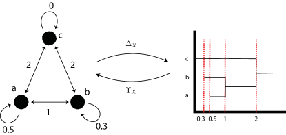
Figure 11: Treegrams and ultra-dissimilarity spaces.

Fix a finite set $X$, denote by $\mathcal{U}^{\mathrm{dis}}(X)$ the collection of all ultra-dissimilarities over $X$ and denote by $\mathcal{T}(X)$ the collection of all treegrams over $X$. We define a map $\Delta_{X}:\mathcal{U}^{\mathrm{dis}}(X)\rightarrow\mathcal{T}(X)$ by sending $u_{X}$ to a treegram $\theta_{X}$ as follows: for each $t\geq 0$, let $\hat{X}_{t}\coloneqq\{x\in X:\,u_{X}(x,x)\leq t\}$ and let $\theta_{X}(t)\coloneqq\left\{[x]_{\mathfrak{c}(t)}^{X}:\,x\in\hat{X}_{t}\right\}$. Note in particular that $\theta_{X}$ satisfies condition (4) of Definition 78 due to the definiteness of $u_{X}$ (cf. condition (3) in Definition 72). Conversely, we define a map $\Upsilon_{X}:\mathcal{T}(X)\rightarrow\mathcal{U}^{\mathrm{dis}}(X)$ as follows. Let $\theta_{X}\in\mathcal{T}(X)$. Then, we define an ultra-dissimilarity $u_{X}\coloneqq\Upsilon_{X}(\theta_{X})$ on $X$ by:

$$u_{X}(x,x^{\prime})\coloneqq\inf\left\{t\geq 0:\,[x]_{t}^{\theta_{X}}=[x^{\prime}]_{t}^{\theta_{X}}\right\},\quad\forall x,x^{\prime}\in X,$$

where $[x]_{t}^{\theta_{X}}\in\theta_{X}(t)$ denotes the block containing $x$. Note that definiteness of $u_{X}$ follows from condition (4) of Definition 78. Then, in analogy to Theorem 14, we have the following theorem. See Figure 11 for an illustration.

Theorem 79.

Given any finite set $X$, $\Delta_{X}:\mathcal{U}^{\mathrm{dis}}(X)\rightarrow\mathcal{T}(X)$ is bijective with inverse $\Upsilon_{X}:\mathcal{T}(X)\rightarrow\mathcal{U}^{\mathrm{dis}}(X)$.

It is obvious that the collection of dendrograms $\mathcal{D}(X)$ over $X$ is a proper subset of $\mathcal{T}(X)$ and that the collection of ultrametrics $\mathcal{U}(X)$ over $X$ is a proper subset of $\mathcal{U}^{\mathrm{dis}}(X)$. Then, Theorem 79 is actually an extension/generalization of Theorem 14.

Via Theorem 79, one can easily represent an ultra-dissimilarity space via a treegram. In particular, see Figure 12 for an illustration of the closed quotient operator via treegrams.

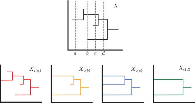
Figure 12: Illustration of Definition 75. We represent a 4-point ultra-dissimilarity space $X$ as a treegram in the first row of the figure. The second row shows the treegrams corresponding to $X_{\mathfrak{c}(t)}$ at different levels $t$.

Appendix C Relegated proofs

C.1 Proofs from Section 3

Proof of Proposition 20.

For any correspondence $R$ between $X$ and $Y$, we have

$$\mathrm{dis}(R,u_{X},u_{Y}) =\sup_{(x,y),(x^{\prime},y^{\prime})\in R}|u_{X}(x,x^{\prime})-u_{Y}(y,y^{\prime})|$$

$$=\sup_{(x,y),(x^{\prime},y^{\prime})\in R}\left|\left((u_{X})^{\frac{1}{p}}(x,x^{\prime})\right)^{p}-\left((u_{Y})^{\frac{1}{p}}(y,y^{\prime})\right)^{p}\right|$$

$$=\left(\mathrm{dis}_{p}\left(R,(u_{X})^{\frac{1}{p}},(u_{Y})^{\frac{1}{p}}\right)\right)^{p}$$

Therefore, by Equation (1) and Equation (9), we have

$$d_{\mathrm{GH}}(X,Y)=\left(d_{\mathrm{GH}}^{\scriptscriptstyle{(p)}}\left(S_{\frac{1}{p}}(X),S_{\frac{1}{p}}(Y)\right)\right)^{p}.$$

Similarly, $\mathrm{dis}_{p}\left(R,u_{X},u_{Y}\right)=\left(\mathrm{dis}\left(R,(u_{X})^{p},(u_{Y})^{p}\right)\right)^{\frac{1}{p}}$ and thus $d_{\mathrm{GH}}^{\scriptscriptstyle{(p)}}(X,Y)=\left(d_{\mathrm{GH}}(S_{p}(X),S_{p}(Y))\right)^{\frac{1}{p}}.$ ∎

Proof of Theorem 26.

Let $Z$ be an ultrametric space such that there exist isometric embeddings $\varphi_{X}:X\hookrightarrow Z$ and $\varphi_{Y}:Y\hookrightarrow Z$. Let $\eta\coloneqq d_{\mathrm{H}}^{Z}(X,Y)$, where we identify $X$ and $Y$ with $\varphi_{X}(X),\varphi_{Y}(Y)\subseteq Z$, respectively. Define $R\coloneqq\{(x,y)\in X\times Y:\,u_{Z}(x,y)\leq\eta\}.$ That $R$ is a correspondence between $X$ and $Y$ follows from the condition that $d_{\mathrm{H}}^{Z}(X,Y)=\eta$ and compactness of $X$ and $Y$. Now, consider any $(x,y),(x^{\prime},y^{\prime})\in R$. Without loss of generality, we assume that $u_{X}(x,x^{\prime})\geq u_{Y}(y,y^{\prime})$. If $u_{X}(x,x^{\prime})=u_{Y}(y,y^{\prime})$, then $\Lambda_{\infty}(u_{X}(x,x^{\prime}),u_{Y}(y,y^{\prime}))=0$. So we further assume that $u_{X}(x,x^{\prime})>u_{Y}(y,y^{\prime})$. Then,

$$\Lambda_{\infty}(u_{X}(x,x^{\prime}),u_{Y}(y,y^{\prime}))=u_{X}(x,x^{\prime})=u_{Z}(x,x^{\prime})$$

$$\leq \max(u_{Z}(x,y),u_{Z}(y,y^{\prime}),u_{Z}(y^{\prime},x^{\prime}))$$

$$\leq \max(u_{Z}(x,y),u_{Z}(x^{\prime},y^{\prime}))\leq\eta.$$

In the second inequality we used the assumption that $u_{X}(x,x^{\prime})>u_{Y}(y,y^{\prime})$. Thus, by taking supremum over all pairs $(x,y),(x^{\prime},y^{\prime})\in R$, one has $\mathrm{dis}_{\infty}(R)\leq\eta.$ Then, we obtain that $u_{\mathrm{GH}}(X,Y)=\inf_{R}\mathrm{dis}_{\infty}(R)\leq d_{\mathrm{GH}}^{\scriptscriptstyle{(\infty)}}(X,Y).$

For the reverse inequality, let $R$ be an arbitrary correspondence between $X$ and $Y$. Let $\eta\coloneqq\mathrm{dis}_{\infty}(R)$. Define a function $u:X\sqcup Y\times X\sqcup Y\rightarrow\mathbb{R}_{\geq 0}$ as follows:

1. $u|_{X\times X}\coloneqq u_{X}$ and $u|_{Y\times Y}\coloneqq u_{Y}$;

2. for any $(x,y)\in X\times Y$, $u(x,y)\coloneqq\inf_{(x^{\prime},y^{\prime})\in R}\max(u_{X}(x,x^{\prime}),u_{Y}(y^{\prime},y),\eta)$;

3. for any $(y,x)\in Y\times X$, $u(y,x)\coloneqq u(x,y)$.

Now we show that $u$ is an ultrametric on the disjoint union $X\sqcup Y$. Because of the symmetric roles of $X$ and $Y$, we only need to verify the following two cases:

Case 1:

$\forall x,x^{\prime}\in X$ and $\forall y\in Y$, $u(x,y)\leq\max(u(x,x^{\prime}),u(x^{\prime},y))$;

Case 2:

$\forall x,x^{\prime}\in X$ and $\forall y\in Y$, $u(x,x^{\prime})\leq\max(u(x,y),u(x^{\prime},y))$.

For Case 1,

$$\max(u(x,x^{\prime}),u(x^{\prime},y)) =\max\left(u(x,x^{\prime}),\inf_{(x_{1},y_{1})\in R}\max(u_{X}(x^{\prime},x_{1}),u_{Y}(y_{1},y),\eta)\right)$$

$$=\inf_{(x_{1},y_{1})\in R}\max\left(u(x,x^{\prime}),u_{X}(x^{\prime},x_{1}),u_{Y}(y_{1},y),\eta\right)$$

$$\geq\inf_{(x_{1},y_{1})\in R}\max\left(u_{X}(x,x_{1}),u_{Y}(y_{1},y),\eta\right)$$

$$=u(x,y).$$

For Case 2,

$$\max\left(\inf_{(x_{1},y_{1})\in R}\max\left(u_{X}(x,x_{1}),u_{Y}(y_{1},y),\eta\right),\inf_{(x_{2},y_{2})\in R}\max\left(u_{X}(x_{2},x^{\prime}),u_{Y}(y_{2},y),\eta\right)\right)$$

$$= \inf_{(x_{1},y_{1}),(x_{2},y_{2})\in R}\max\left(u_{X}(x,x_{1}),u_{Y}(y_{1},y),\eta,u_{X}(x_{2},x^{\prime}),u_{Y}(y_{2},y),\eta\right)$$

$$\geq \inf_{(x_{1},y_{1}),(x_{2},y_{2})\in R}\max\left(u_{X}(x,x_{1}),u_{X}(x_{2},x^{\prime}),u_{Y}(y_{1},y_{2}),\eta\right)$$

$$\geq \inf_{(x_{1},y_{1}),(x_{2},y_{2})\in R}\max\left(u_{X}(x,x_{1}),u_{X}(x_{2},x^{\prime}),u_{X}(x_{1},x_{2})\right)\geq u_{X}(x,x^{\prime})=u(x,x^{\prime}).$$

The second inequality above follows from the fact that $\Lambda_{\infty}(u_{X}(x_{1},x_{2}),u_{Y}(y_{1},y_{2}))\leq\mathrm{dis}_{\infty}(R)=\eta$ and Equation (7).

Note that $u(x,y)=\eta$ for every $(x,y)\in R$. Therefore, $d_{\mathrm{GH}}^{\scriptscriptstyle{(\infty)}}(X,Y)\leq d_{\mathrm{H}}^{(X\sqcup Y,u)}(X,Y)=\eta$. This implies that $d_{\mathrm{GH}}^{\scriptscriptstyle{(\infty)}}(X,Y)\leq\inf_{R}\mathrm{dis}_{\infty}(R)=u_{\mathrm{GH}}(X,Y).$ ∎

C.2 Proofs from Section 5

C.2.1 Proof of Theorem 34 (Time complexity of Algorithm $\mathbf{FindCorrRec}$ (Algorithm 2))

Lemma 80 (Inheritance of the FGC).

Let $X$ and $Y$ be finite ultrametric spaces such that $X,Y\in\mathcal{U}_{1}(\varepsilon,\gamma)$. Assume that $0\leq\mathrm{diam}(Y)-\mathrm{diam}(X)\leq\varepsilon$ and that $\mathrm{diam}(Y)>\varepsilon$. Write $X_{\mathfrak{o}\left(\delta_{\varepsilon}(Y)\right)}=\{X_{i}\}_{i\in[N_{X}]}$ and $Y_{\mathfrak{o}\left(\delta_{0}(Y)\right)}=\{Y_{j}\}_{j\in[N_{Y}]}$. Then, given any surjection $\Psi:[N_{X}]\twoheadrightarrow[N_{Y}]$, for each $j\in[N_{Y}]$, we have that $X_{\Psi^{-1}(j)}\in\mathcal{U}_{1}(\varepsilon,\gamma)$ and $Y_{j}\in\mathcal{U}_{1}(\varepsilon,\gamma)$.

Proof.

For notational simplicity, let $\delta_{0}\coloneqq\delta_{0}(Y)$ and let $\delta_{\varepsilon}\coloneqq\delta_{\varepsilon}(Y)$.

We first prove that $Y_{j}\in\mathcal{U}_{1}(\varepsilon,\gamma)$. For any $y\in Y_{j}$, note that $Y_{j}=[y]_{\mathfrak{o}(\delta_{0})}^{Y}$. Given any $t\geq\varepsilon$, if $t\leq\delta_{0}$, then we easily see that $[y]_{\mathfrak{o}(t-\varepsilon)}^{Y_{j}}=[y]_{\mathfrak{o}(t-\varepsilon)}^{Y}.$ Then,

$$\#[y]_{\mathfrak{c}(t)}^{Y_{j}}\leq\underbrace{\#[y]_{\mathfrak{c}(t)}^{Y}\leq\gamma\cdot\#[y]_{\mathfrak{o}(t-\varepsilon)}^{Y}}_{\text{FGC}}=\gamma\cdot\#[y]_{\mathfrak{o}(t-\varepsilon)}^{Y_{j}}.$$

Otherwise, if $t>\delta_{0}$, we then have that $[y]_{\mathfrak{c}(t)}^{Y_{j}}=Y_{j}=[y]_{\mathfrak{c}(\delta_{0})}^{Y_{j}}$. Then,

$$\#[y]_{\mathfrak{c}(t)}^{Y_{j}}=\#[y]_{\mathfrak{c}(\delta_{0})}^{Y_{j}}\leq\gamma\cdot\#[y]_{\mathfrak{o}(\delta_{0}-\varepsilon)}^{Y_{j}}\leq\gamma\cdot\#[y]_{\mathfrak{o}(t-\varepsilon)}^{Y_{j}},$$

where the first inequality follows from the previous case $t\leq\delta_{0}$. Therefore, $Y_{j}\in\mathcal{U}_{1}(\varepsilon,\gamma)$.

We then prove that $X_{\Psi^{-1}(j)}\in\mathcal{U}_{1}(\varepsilon,\gamma)$. For $X_{\Psi^{-1}(j)}$, we choose any $x\in X_{\Psi^{-1}(j)}$ and any $t\geq\varepsilon$. If $t\leq\mathrm{diam}(X)$, then it is easy to see that $t-\varepsilon<\delta_{\varepsilon}$. Therefore, $[x]_{\mathfrak{o}(t-\varepsilon)}^{X_{\Psi^{-1}(j)}}=[x]_{\mathfrak{o}(t-\varepsilon)}^{X}$ and thus

$$\#[x]_{\mathfrak{c}(t)}^{X_{\Psi^{-1}(j)}}\leq\underbrace{\#[x]_{\mathfrak{c}(t)}^{X}\leq\gamma\cdot\#[x]_{\mathfrak{o}(t-\varepsilon)}^{X}}_{\text{FGC}}=\gamma\cdot\#[x]_{\mathfrak{o}(t-\varepsilon)}^{X_{\Psi^{-1}(j)}}.$$

If $t>\mathrm{diam}(X)$, then we have that $[x]_{\mathfrak{c}(t)}^{X_{\Psi^{-1}(j)}}=X_{\Psi^{-1}(j)}=[x]_{\mathfrak{c}(\mathrm{diam}(X))}^{X_{\Psi^{-1}(j)}}$. Then,

$$\#[x]_{\mathfrak{c}(t)}^{X_{\Psi^{-1}(j)}}=\#[x]_{\mathfrak{c}(\mathrm{diam}(X))}^{X_{\Psi^{-1}(j)}}\leq\gamma\cdot\#[x]_{\mathfrak{o}(\mathrm{diam}(X)-\varepsilon)}^{X_{\Psi^{-1}(j)}}\leq\gamma\cdot\#[x]_{\mathfrak{o}(t-\varepsilon)}^{X_{\Psi^{-1}(j)}},$$

where the first inequality follows from the previous case $t\leq\mathrm{diam}(X)$. Therefore, $X_{\Psi^{-1}(j)}\in\mathcal{U}_{1}(\varepsilon,\gamma)$.

∎

In this way, the inputs to each subproblem encountered while running Algorithm 2 will satisfy the first $(\varepsilon,\gamma)$-growth condition. This justifies the analysis presented below regarding the number and the size of subproblems.

Proof of Theorem 34.

We are going to invoke the master theorem [12] in order to analyze the complexity of our recursive algorithm (Algorithm 2).

Number of subproblems

By the FGC (or Remark 33), we have that $\max(N_{X},N_{Y})\leq\gamma$. There will be at most $\gamma^{\gamma}$ surjections $\Psi:[N_{X}]\twoheadrightarrow[N_{Y}]$. For each such a surjection, Algorithm 2 inspects $N_{Y}$ ($\leq\gamma$) subproblems. Therefore, there are at most $\gamma^{\gamma+1}$ subproblems.

Size of a subproblem

Fix a surjection $\Psi:[N_{X}]\twoheadrightarrow[N_{Y}]$. For each $k\in[N_{Y}]$, we write $Y_{k}\coloneqq[y_{k}]_{\mathfrak{o}\left(\delta_{0}\right)}^{Y}$ for some $y_{k}\in Y$. Then, for a fixed $j\in[N_{Y}]$, we have that

$$\#Y=\#[y_{j}]_{\mathfrak{o}\left(\delta_{0}\right)}^{Y}+\sum_{k\in[N_{Y}]\backslash\{j\}}\#[y_{k}]_{\mathfrak{o}\left(\delta_{0}\right)}^{Y}\geq\#Y_{j}+\frac{M-1}{\gamma}\cdot\#Y,$$

where the last inequality follows from the FGC and the fact that $[y_{k}]_{{\delta_{0}+\varepsilon}}^{Y}=Y$ for each $k\in[N_{Y}]$. Therefore, $\#Y_{j}\leq\left(1-\frac{M-1}{\gamma}\right)\cdot\#Y$. Now, regarding $X_{\Psi^{-1}(j)}$, since $\Psi$ is a surjection and $M\geq 2$, there exists $i\notin\Psi^{-1}(j)$ such that $X_{i}\bigcap X_{\Psi^{-1}(j)}=\emptyset$. Assume $X_{i}=[x_{i}]_{\mathfrak{o}\left(\delta_{\varepsilon}\right)}^{X}$ for some $x_{i}\in X$. Then,

$$\#[x_{i}]^{X}_{\mathfrak{o}\left(\delta_{\varepsilon}\right)}\geq\frac{\#[x_{i}]^{X}_{\mathfrak{c}\left(\delta_{\varepsilon}+\varepsilon\right)}}{\gamma}\geq\frac{\#[x_{i}]^{X}_{\mathfrak{o}\left(\delta_{\varepsilon}+\varepsilon\right)}}{\gamma}\geq\frac{\#[x_{i}]^{X}_{\mathfrak{c}\left(\delta_{\varepsilon}+2\varepsilon\right)}}{\gamma^{2}}=\frac{\#X}{\gamma^{2}},$$

where the last equality follows from the fact that $\delta_{\varepsilon}+2\varepsilon=\mathrm{diam}(Y)+\varepsilon>\mathrm{diam}(X)$. Therefore,

$$\#X_{\Psi^{-1}(j)}\leq\#X-\#X_{i}\left(1-\frac{1}{\gamma^{2}}\right)\#X.$$

When $\gamma\geq 1$, we have that $1-\frac{1}{\gamma^{2}}\geq 1-\frac{M-1}{\gamma}$. So, $\max(\#X_{\Psi^{-1}(j)},\#Y_{j})\leq\left(1-\frac{1}{\gamma^{2}}\right)n$ and thus the size of a subproblem is bounded above by $\left(1-\frac{1}{\gamma^{2}}\right)n$.

Base case complexity and other work

If $(X,Y,\varepsilon)$ is one of the base cases, it takes time at most $O(n^{2})$ in order to either directly generate a correspondence or 0. In order to utilize the results from the subproblems, we need at most $O(n^{2})$ time to construct distance matrices $u_{X}$ and $u_{Y}$ from TDSs in order to implement the unions $X_{\Psi^{-1}(j)}$ (cf. Appendix A). It then takes time at most $O(n^{2})$ in total to construct all the unions $X_{\Psi^{-1}(j)}$, $R_{j}$ and $R$, and to transpose $R$ when/if needed.

Conclusion

Denote by $W(n)$ the time complexity of the algorithm where $n=\max(\#X,\#Y)$. Then,

$$W(n)\leq\gamma^{\gamma+1}\cdot W\left(\frac{n}{\gamma^{2}/(\gamma^{2}-1)}\right)+O\left(n^{2}\right).$$

Since by assumption that $\gamma\geq 2$, the critical exponent $\log_{\frac{\gamma^{2}}{\gamma^{2}-1}}{\gamma^{\gamma+1}}$ is strictly greater than 2. Therefore, by the master theorem we have that $W(n)=O\left(n^{(\gamma+1)\log_{\mathrm{b}(\gamma)}{\gamma}}\right).$ This concludes the proof. ∎

C.2.2 Proof of Proposition 37

In the following lemmas, we will always assume that $X$ and $Y$ are finite ultrametric spaces and that there exists $\varepsilon\geq 0$ such that $\mathrm{diam}(X)>\varepsilon$ and $\mathrm{diam}(Y)\leq\varepsilon$.

Lemma 81.

There exists an $\varepsilon$-correspondence between $X$ and $Y$ if and only if there exists an $\varepsilon$-correspondence between $X_{\mathfrak{c}\left(\varepsilon\right)}$ and $Y$.

Proof.

Suppose that $R$ is an $\varepsilon$-correspondence between $X$ and $Y$. Then, we define the set $R_{\varepsilon}\subseteq X_{\mathfrak{c}\left(\varepsilon\right)}\times Y$ as follows:

$$R_{\varepsilon}\coloneqq\left\{\left([x]_{\mathfrak{c}(\varepsilon)}^{X},y\right)\in X_{\mathfrak{c}\left(\varepsilon\right)}\times Y:\,(x,y)\in R\right\}.$$

It is easy to verify that $R_{\varepsilon}$ is a correspondence between $X_{\mathfrak{c}\left(\varepsilon\right)}$ and $Y$. Now, for any two pairs $\left([x]_{\mathfrak{c}(\varepsilon)}^{X},y\right),\left([x^{\prime}]_{\mathfrak{c}(\varepsilon)}^{X},y^{\prime}\right)\in R_{\varepsilon}$, we have the following:

$$\left|u_{X_{\mathfrak{c}\left(\varepsilon\right)}}\left([x]_{\mathfrak{c}(\varepsilon)}^{X},[x^{\prime}]_{\mathfrak{c}(\varepsilon)}^{X}\right)-u_{Y}(y,y^{\prime})\right| =\begin{cases}\left|u_{X}(x,x^{\prime})-u_{Y}(y,y^{\prime})\right|&\mbox{if $[x]_{\mathfrak{c}(\varepsilon)}^{X}\neq[x^{\prime}]_{\mathfrak{c}(\varepsilon)}^{X}$}\\ u_{Y}(y,y^{\prime})&\mbox{if $[x]_{\mathfrak{c}(\varepsilon)}^{X}=[x^{\prime}]_{\mathfrak{c}(\varepsilon)}^{X}$}\end{cases}$$

$$\leq\begin{cases}\mathrm{dis}(R)&\mbox{if $[x]_{\mathfrak{c}(\varepsilon)}^{X}\neq[x^{\prime}]_{\mathfrak{c}(\varepsilon)}^{X}$}\\ \mathrm{diam}(Y)&\mbox{if $[x]_{\mathfrak{c}(\varepsilon)}^{X}=[x^{\prime}]_{\mathfrak{c}(\varepsilon)}^{X}$}\end{cases}\leq\varepsilon$$

Therefore, $\mathrm{dis}(R_{\varepsilon})\leq\varepsilon$ and thus $R_{\varepsilon}$ is an $\varepsilon$-correspondence between $X_{\mathfrak{c}\left(\varepsilon\right)}$ and $Y$.

Now for the converse, suppose that there exists an $\varepsilon$-correspondence $R_{\varepsilon}$ between $X_{\mathfrak{c}\left(\varepsilon\right)}$ and $Y$. Then, we define $R\subseteq X\times Y$ as follows:

$$R\coloneqq\left\{(x,y)\in X\times Y:\left([x]_{\mathfrak{c}(\varepsilon)}^{X},y\right)\in R\right\}.$$

It is easy to verify that $R$ is a correspondence between $X$ and $Y$. Then, for any $(x,y),(x^{\prime},y^{\prime})\in R$, if $[x]_{\mathfrak{c}(\varepsilon)}^{X}\neq[x^{\prime}]_{\mathfrak{c}(\varepsilon)}^{X}$, we have

$$|u_{X}(x,x^{\prime})-u_{Y}(y,y^{\prime})|\leq\left|u_{X_{\mathfrak{c}\left(\varepsilon\right)}}\left([x]_{\mathfrak{c}(\varepsilon)}^{X},[x^{\prime}]_{\mathfrak{c}(\varepsilon)}^{X}\right)-u_{Y}(y,y^{\prime})\right|\leq\mathrm{dis}(R_{\varepsilon})\leq\varepsilon.$$

If $[x]_{\mathfrak{c}(\varepsilon)}^{X}=[x^{\prime}]_{\mathfrak{c}(\varepsilon)}^{X}$, then $u_{X}(x,x^{\prime})\leq\varepsilon$. Moreover, $u_{Y}(y,y^{\prime})\leq\mathrm{diam}(Y)\leq\varepsilon$. Then, $|u_{X}(x,x^{\prime})-u_{Y}(y,y^{\prime})|\leq\varepsilon$. Therefore, $\mathrm{dis}(R)\leq\varepsilon$ and thus $R$ is an $\varepsilon$-correspondence between $X$ and $Y$. This concludes the proof. ∎

Lemma 82.

For any $\varepsilon$-correspondence $R_{\varepsilon}$ between $X_{\mathfrak{c}\left(\varepsilon\right)}$ and $Y$, there exists a surjection $\psi$ from $Y$ to $X_{\mathfrak{c}\left(\varepsilon\right)}$ such that $R_{\varepsilon}=\{(\psi(y),y):\,y\in Y\}$.

Proof.

We first show that if $\left([x]_{\mathfrak{c}(\varepsilon)}^{X},y\right),([x^{\prime}]_{\mathfrak{c}(\varepsilon)}^{X},y)\in R_{\varepsilon}$, then $[x]_{\mathfrak{c}(\varepsilon)}^{X}=[x^{\prime}]_{\mathfrak{c}(\varepsilon)}^{X}$. Otherwise, suppose that $[x]_{\mathfrak{c}(\varepsilon)}^{X}\neq[x^{\prime}]_{\mathfrak{c}(\varepsilon)}^{X}$, which is equivalent to the condition that $u_{X}(x,x^{\prime})>\varepsilon$. Then,

$$\varepsilon\geq\mathrm{dis}(R_{\varepsilon})\geq\big{|}u_{X_{\mathfrak{c}\left(\varepsilon\right)}}\left([x]_{\mathfrak{c}(\varepsilon)}^{X},[x^{\prime}]_{\mathfrak{c}(\varepsilon)}^{X}\right)-u_{Y}(y,y)\big{|}=u_{X}(x,x^{\prime})>\varepsilon,$$

which is a contradiction! Then, $R_{\varepsilon}$ naturally induces a well-defined map $\psi:Y\rightarrow X_{\mathfrak{c}\left(\varepsilon\right)}$ taking $y\in Y$ to $[x]_{\mathfrak{c}(\varepsilon)}^{X}$ such that $\left([x]_{\mathfrak{c}(\varepsilon)}^{X},y\right)\in R_{\varepsilon}$. It is easy to check that $\psi$ is surjective and that $R_{\varepsilon}=\{(\psi(y),y):\,y\in Y\}$. ∎

Recall from Section 5.2.5 that $\mathrm{sep}(X)\coloneqq\min\{d_{X}(x,x^{\prime}):\,x,x^{\prime}\in X\text{ and }x\neq x^{\prime}\}$ denotes the separation of a finite metric space $(X,d_{X})$.

Lemma 83.

Assume that $\mathrm{sep}(X)>\varepsilon$. Then any injective map $\varphi:X\rightarrow Y$ with $\mathrm{dis}(\varphi)\leq\varepsilon$ induces an $\varepsilon$-correspondence between $X$ and $Y$.

Proof.

Suppose $X=\{x_{1},\ldots,x_{n}\}$ and $\mathrm{im}(\varphi)=\{y_{1},\ldots,y_{n}\}$ where $y_{i}=\varphi(x_{i})$ for every $i=1,\ldots,n$. For any $y\in Y$, define

$$i_{y}\coloneqq\min\left\{\mathop{\mathrm{argmin}}_{j=1,\ldots,n}u_{Y}(y,y_{j})\right\}.$$

Obviously, $i_{y_{j}}=j$. Then, we define $R\subseteq X\times Y$ as follows:

$$R\coloneqq\{(x_{i_{y}},y)\in X\times Y:\,\forall y\in Y\}.$$

It is easy to check that $R$ is a correspondence. Now, we verify that $\mathrm{dis}(R)\leq\varepsilon$. Let $(x_{i},y),(x_{j},y^{\prime})\in R$, where $i=i_{y}$ and $j=i_{y^{\prime}}$. If $i=j$, then $|u_{X}(x_{i},x_{i})-u_{Y}(y,y^{\prime})|=u_{Y}(y,y^{\prime})\leq\mathrm{diam}(Y)\leq\varepsilon.$ Now assume $i\neq j$. It is obvious that $(x_{i},y_{i}),(x_{j},y_{j})\in R$ and thus $u_{X}(x_{i},x_{j})-u_{Y}(y_{i},y_{j})\leq\mathrm{dis}(\varphi)\leq\varepsilon$. Since $u_{X}(x_{i},x_{j})-u_{Y}(y,y^{\prime})\geq\mathrm{sep}(X)-\mathrm{diam}(Y)\geq 0$, the inequality $|u_{X}(x_{i},x_{j})-u_{Y}(y,y^{\prime})|\leq\varepsilon$ follows from the following observation:

Claim 84.

For $y,y^{\prime}\in Y$, if $i_{y}\neq i_{y^{\prime}}$, then $u_{Y}(y,y^{\prime})\geq u_{Y}(y_{i},y_{j})$ where $i\coloneqq i_{y}$ and $j\coloneqq i_{y^{\prime}}$.

Proof of Claim 84.

Suppose otherwise that $u_{Y}(y,y^{\prime})<u_{Y}(y_{i},y_{j})$. If $u_{Y}(y_{i},y)\leq u_{Y}(y,y^{\prime})$, then

$$u_{Y}(y^{\prime},y_{i})\leq\max(u_{Y}(y,y^{\prime}),u_{Y}(y,y_{i}))\leq u_{Y}(y,y^{\prime}).$$

By definition of $j=i_{y^{\prime}}$, we have that $u_{Y}(y_{j},y^{\prime})\leq u_{Y}(y_{i},y^{\prime})\leq u_{Y}(y,y^{\prime})$. Then, $u_{Y}(y_{i},y_{j})\leq\max(u_{Y}(y_{i},y^{\prime}),u_{Y}(y^{\prime},y_{j}))\leq u_{Y}(y,y^{\prime})$, which is a contradiction. Therefore, $u_{Y}(y_{i},y)>u_{Y}(y,y^{\prime})$ and similarly $u_{Y}(y_{j},y^{\prime})>u_{Y}(y,y^{\prime})$. Then, by the strong triangle inequality we have that $u_{Y}(y,y_{i})=u_{Y}(y^{\prime},y_{i})$ and $u_{Y}(y,y_{j})=u_{Y}(y^{\prime},y_{j})$. By definition of $i=i_{y}$ and $j=i_{y^{\prime}}$, we have that

$$u_{Y}(y,y_{j})=u_{Y}(y^{\prime},y_{j})\leq u_{Y}(y^{\prime},y_{i})=u_{Y}(y,y_{i}),$$

which implies that $j\in\mathop{\mathrm{argmin}}_{k=1,\ldots,n}u_{Y}(y,y_{k})$ and thus $j>i$. However, we can similarly prove that $i>j$, which is a contradiction. Therefore, $u_{Y}(y,y^{\prime})\geq u_{Y}(y_{i},y_{j})$. ∎

∎

Proof of Proposition 37.

By Lemma 81, we only need to prove that there exists an $\varepsilon$-correspondence between $X_{\mathfrak{c}\left(\varepsilon\right)}$ and $Y$ if and only if there exists an injective map $\varphi:X_{\mathfrak{c}\left(\varepsilon\right)}\rightarrow Y$ with $\mathrm{dis}(\varphi)\leq\varepsilon.$

Assuming the existence of such a correspondence $R_{\varepsilon}$, then by Lemma 82, there exists a surjection $\psi:Y\twoheadrightarrow X_{\mathfrak{c}\left(\varepsilon\right)}$ such that $R_{\varepsilon}=\{(\psi(y),y):y\in Y\}$. Then, we construct an injective map $\varphi:X_{\mathfrak{c}\left(\varepsilon\right)}\rightarrow Y$ by mapping each $[x]_{\mathfrak{c}(\varepsilon)}^{X}\in X_{\mathfrak{c}\left(\varepsilon\right)}$ to $y$, where $y$ is arbitrarily chosen from $\psi^{-1}\left([x]_{\mathfrak{c}(\varepsilon)}^{X}\right)$. Then, $\mathrm{dis}(\varphi)\leq\mathrm{dis}(\psi)\leq\varepsilon.$

Now, assume that there exists an injective map $\varphi:X_{\mathfrak{c}\left(\varepsilon\right)}\rightarrow Y$ with $\mathrm{dis}(\varphi)\leq\varepsilon.$ Obviously, we have $\mathrm{sep}(X_{\mathfrak{c}\left(\varepsilon\right)})>\varepsilon$, and thus, by Lemma 83, there exists a correspondence $R_{\varepsilon}$ between $X_{\mathfrak{c}\left(\varepsilon\right)}$ and $Y$ with $\mathrm{dis}(R_{\varepsilon})\leq\varepsilon$. ∎

C.2.3 Proof of Remark 35

We first establish the following characterization of elements in $V_{X}^{(\varepsilon)}$.

Lemma 85.

Let $X$ be a finite ultrametric space and let $\varepsilon\geq 0$. Then, a subset $U^{X}\subseteq X$ belongs to $V_{X}^{(\varepsilon)}$ if and only if $U^{X}$ contains all $x\in X$ such that $u_{X}\left(x,U^{X}\right)<\mathrm{diam}\left(U^{X}\right)-2\varepsilon$, where $u_{X}\left(x,U^{X}\right)\coloneqq\min\left\{u_{X}(x,x^{\prime}):\,x^{\prime}\in U^{X}\right\}$.

Proof.

If $U^{X}\in V_{X}^{(\varepsilon)}$, then $U^{X}$ is an $\varepsilon$-maximal union of closed balls in $B^{X}\subseteq X$ (cf. Section 5.2.3): write $B^{X}_{\mathfrak{o}\left(\rho_{\varepsilon}\left(B^{X}\right)\right)}=\{B_{1}^{X},\ldots,B_{N}^{X}\}$, where $\rho_{\varepsilon}\left(B^{X}\right)\coloneqq\max\left(\mathrm{diam}\left(B^{X}\right)-2\varepsilon,0\right)$; then, $U^{X}=\bigcup_{i\in I}B^{X}_{i}$ for some non-empty $I\subseteq\{1,\ldots,N\}$ and $U^{X}$ satisfies that $\mathrm{diam}\left(U^{X}\right)=\mathrm{diam}\left(B^{X}\right)$. Without loss of generality, we assume that $\mathrm{diam}\left(U^{X}\right)-2\varepsilon>0$. Given any $x\in X$ such that $u_{X}\left(x,U^{X}\right)<\mathrm{diam}\left(U^{X}\right)-2\varepsilon$, there exists $x^{\prime}\in U^{X}$ such that $u_{X}(x,x^{\prime})<\mathrm{diam}\left(U^{X}\right)-2\varepsilon=\mathrm{diam}(B^{X})-2\varepsilon$. Since $x^{\prime}\in U^{X}\subseteq B^{X}$, $x^{\prime}\in B^{X}_{i}$ for some $i\in I$. Then,

$$B^{X}_{i}=[x^{\prime}]^{X}_{\mathfrak{o}\left(\rho_{\varepsilon}\left(B^{X}\right)\right)}=\{x^{\prime\prime}\in X:\,u_{X}(x^{\prime},x^{\prime\prime})<\mathrm{diam}(B^{X})-2\varepsilon\}.$$

Therefore, $x\in B^{X}_{i}\subseteq U^{X}$.

Now, let $U^{X}\subseteq X$ be a subset containing all $x\in X$ such that $u_{X}\left(x,U^{X}\right)<\mathrm{diam}\left(U^{X}\right)-2\varepsilon$. For any $x\in U^{X}$, consider the ball $B^{X}\coloneqq[x]^{X}_{\mathfrak{c}(\delta)}$, where $\delta\coloneqq\mathrm{diam}\left(U^{X}\right)$. It is obvious that $U^{X}\subseteq B^{X}$ and $\mathrm{diam}(U^{X})=\mathrm{diam}(B^{X})$. If $\mathrm{diam}\left(U^{X}\right)\leq 2\varepsilon$, then $\rho_{\varepsilon}(B^{X})=0$. Therefore, $B^{X}_{\mathfrak{o}\left(\rho_{\varepsilon}\left(B^{X}\right)\right)}=\{\{x\}:\,x\in B^{X}\}$ and thus obviously, $U^{X}\in B^{X}_{(\varepsilon)}\subseteq V_{X}^{(\varepsilon)}$. Now, assume that $\mathrm{diam}\left(U^{X}\right)>2\varepsilon$. Then, $\rho_{\varepsilon}(B^{X})=\mathrm{diam}(B^{X})-2\varepsilon=\mathrm{diam}\left(U^{X}\right)-2\varepsilon$. By assumption we have that for each $x\in U^{X}$

$$[x]^{X}_{\mathfrak{o}\left(\rho_{\varepsilon}\left(B^{X}\right)\right)}=\{x^{\prime}\in X:\,u_{X}(x,x^{\prime})<\mathrm{diam}\left(U^{X}\right)-2\varepsilon\}\subseteq U^{X}.$$

This implies that

$$U^{X}=\bigcup_{x\in U^{X}}[x]^{X}_{\mathfrak{o}\left(\rho_{\varepsilon}\left(B^{X}\right)\right)}.$$

So $U^{X}$ is the union of some elements in $B^{X}_{\mathfrak{o}\left(\rho_{\varepsilon}\left(B^{X}\right)\right)}$ and thus $U^{X}\in B^{X}_{(\varepsilon)}\subseteq V_{X}^{(\varepsilon)}$. ∎

Proof of Remark 35.

Let $U^{X}\in V_{X}^{(\varepsilon)}$ and let $B^{Y}\in V_{Y}$ be such that $|\mathrm{diam}\left(U^{X}\right)-\mathrm{diam}\left(B^{Y}\right)|\leq\varepsilon$ and $\mathrm{diam}\left(B^{Y}\right)>\varepsilon$. Let $U^{X}_{\mathfrak{o}\left(\delta_{\varepsilon}\left(B^{Y}\right)\right)}=\left\{U^{X}_{1},\ldots,U^{X}_{N_{U_{X}}}\right\}$. For any subset $I\subseteq[N_{U_{X}}]$ (which can be a singleton), we will prove next that the union $U^{X}_{I}\coloneqq\bigcup_{i\in I}U^{X}_{i}$ belongs to $V_{X}^{(\varepsilon)}$. For any $x\in X$, suppose that there is $x^{\prime}\in U^{X}_{i}\subseteq U^{X}_{I}$ such that $u_{X}(x,x^{\prime})<\mathrm{diam}(U^{X}_{I})-2\varepsilon\leq\mathrm{diam}\left(U^{X}\right)-2\varepsilon$. Then, $x\in U^{X}$ since $U^{X}\in V_{X}^{(\varepsilon)}$ (cf. Lemma 85). Now, $u_{X}(x,x^{\prime})<\mathrm{diam}(U^{X}_{I})-2\varepsilon\leq\mathrm{diam}\left(U^{X}\right)-2\varepsilon\leq\delta_{\varepsilon}\left(B^{Y}\right)$. So $x$ and $x^{\prime}$ belong to the same block in $U^{X}_{\mathfrak{o}\left(\delta_{\varepsilon}\left(B^{Y}\right)\right)}$ and thus $x\in U^{X}_{i}$. Therefore, $x\in U^{X}_{I}$ and thus by Lemma 85 we have that $U^{X}_{I}\in V_{X}^{(\varepsilon)}$. ∎

C.2.4 Proof of Theorem 38 (correctness of Algorithm $\mathbf{FindCorrDP}$ (Algorithm 4))

Proof.

We prove a more general result, namely that for any $\left(U^{X},B^{Y}\right)\in V_{X}^{(\varepsilon)}\times V_{Y}$, $\mathrm{DYN}\left(U^{X},B^{Y}\right)=1$ if and only if there exists an $\varepsilon$-correspondence between $U^{X}$ and $B^{Y}$.

If $\left(U^{X},B^{Y}\right)$ belongs to one of the base cases, the statement is obviously true. For non-base cases, we prove the claim by induction on $\mathrm{diam}\left(B^{Y}\right)\in\mathrm{spec}(Y)$. For this, we exploit the fact that the spectrum $\mathrm{spec}(Y)=\{0=t_{0}<\cdots<t_{M}=\mathrm{diam}(Y)\}$ is a finite set. When $\mathrm{diam}\left(B^{Y}\right)=t_{0}=0$, for any $U^{X}$, $\left(U^{X},B^{Y}\right)$ belongs to one of the base cases, so the statement holds true trivially. Let $1<i_{0}\leq M$ and suppose that the claim holds true for all $t_{i}$ when $i<i_{0}$ and all $\mathrm{DYN}\left(U^{X},B^{Y}\right)$ are known whenever $\mathrm{diam}\left(B^{Y}\right)<t_{i_{0}}$. Then, the induction step follows directly from Theorem 4 and Proposition 37. We elaborate this via the two cases described in page 5.2.3 as follows:

1. If $\mathrm{diam}\left(B^{Y}\right)>\varepsilon$, Algorithm $\mathbf{FindCorrDP}$ partitions $U^{X}$ and $B^{Y}$ to obtain $U^{X}_{\mathfrak{o}\left(\delta_{\varepsilon}\left(B^{Y}\right)\right)}=\{U^{X}_{i}\}_{i\in[N_{U_{X}}]}$ and $B^{Y}_{\mathfrak{o}\left({\delta_{0}\left(B^{Y}\right)}\right)}=\{B^{Y}_{j}\}_{j\in[N_{B_{Y}}]}$, respectively. It is obvious that $B^{Y}_{j}\in V_{Y}$ for each $j\in[N_{B_{Y}}]$, and by Remark 35 we know that $U^{X}_{i}\in V_{X}^{(\varepsilon)}$ for each $i\in[N_{U_{X}}]$. Since $\mathrm{diam}(B_{j}^{Y})<\mathrm{diam}\left(B^{Y}\right)=t_{i_{0}}$ for each $j\in[N_{B_{Y}}]$, by the induction assumption, the value $\mathrm{DYN}\left(U^{X}_{\Psi^{-1}(j)},B^{Y}_{j}\right)$ has already been computed for any surjection $\Psi:[N_{U_{X}}]\rightarrow[N_{B_{Y}}]$ so we already know whether or not there exists any $\varepsilon$-correspondence between $U^{X}_{\Psi^{-1}(j)}$ and $B^{Y}_{j}$. $\mathrm{DYN}\left(U^{X},B^{Y}\right)$ is then determined via Theorem 4: this value is 1 if there exists an $\varepsilon$-correspondence between $U^{X}$ and $B^{Y}$, and is 0 otherwise.

2. If $\mathrm{diam}\left(B^{Y}\right)\leq\varepsilon$, Algorithm $\mathbf{FindCorrDP}$ assigns the value $\mathbf{FindCorrSmall}(U^{X},B^{Y},\varepsilon)$ to $\mathrm{DYN}\left(U^{X},B^{Y}\right)$. Then, due to Proposition 37, $\mathrm{DYN}\left(U^{X},B^{Y}\right)=1$ if and only if there exists an $\varepsilon$-correspondence between $U^{X}$ and $B^{Y}$.

Since we know that $X$ and $Y$ are at the end of the arrays $\mathrm{LX}^{(\varepsilon)}$ and $\mathrm{LY}$, respectively, then $\mathrm{DYN}(\mathrm{END},\mathrm{END})=1$ if and only if there exists an $\varepsilon$-correspondence between $X$ and $Y$. ∎

C.2.5 Proof of Remark 42

Proof.

Let $X$ be a finite ultrametric space such that $X\in\mathcal{U}_{2}(\varepsilon,\gamma)$ for some $\varepsilon\geq 0$ and $\gamma\geq 1$. For any $x\in X$ and any $r>\mathrm{diam}(X)$, we have that ${B}_{r}(x)=X={B}_{\mathrm{diam}(X)}(x)$. So if ${B}_{\mathrm{diam}(X)}(x)$ can be covered by $K$ many balls with radius $\frac{\mathrm{diam}(X)}{2}$, then it is obvious that ${B}_{r}(x)$ can also be covered by $K$ balls with radius $\frac{r}{2}>\frac{\mathrm{diam}(X)}{2}$. Therefore, to determine the doubling constant of $X$, we only need to consider a radius $r$ within the range $(0,\mathrm{diam}(X)]$. Let $k=\lfloor\frac{r}{4\varepsilon}\rfloor+1$, then $k$ is the unique integer such that $r-2\varepsilon\cdot k<\frac{r}{2}\leq r-2\varepsilon\cdot(k-1)$. We assume that $r-2\varepsilon\cdot k\geq 0$ (the case when $r-2\varepsilon\cdot k<0$ can be proved similarly and we omit the details). Then, by the SGC we have that

$$\#\left\{[x^{\prime}]_{\mathfrak{c}\left(\frac{r}{2}\right)}:\,x^{\prime}\in[x]_{\mathfrak{c}\left({r}\right)}\right\} \leq\#\left\{[x^{\prime}]_{\mathfrak{c}\left({r-2\varepsilon\cdot k}\right)}:\,x^{\prime}\in[x]_{\mathfrak{c}\left({r}\right)}\right\}\leq\#\left\{[x^{\prime}]_{\mathfrak{o}\left({r-2\varepsilon\cdot k}\right)}:\,x^{\prime}\in[x]_{\mathfrak{c}\left({r}\right)}\right\}$$

$$\leq\gamma\cdot\#\left\{[x^{\prime}]_{\mathfrak{c}\left({r-2\varepsilon\cdot(k-1)}\right)}:\,x^{\prime}\in[x]_{\mathfrak{c}\left({r}\right)}\right\}\leq\gamma\cdot\#\left\{[x^{\prime}]_{\mathfrak{o}\left({r-2\varepsilon\cdot(k-1)}\right)}:\,x^{\prime}\in[x]_{\mathfrak{c}\left({r}\right)}\right\}$$

$$\leq\cdots\leq\gamma^{k-1}\cdot\#\left\{[x^{\prime}]_{\mathfrak{c}\left({r-2\varepsilon}\right)}:\,x^{\prime}\in[x]_{\mathfrak{c}\left({r}\right)}\right\}\leq\gamma^{k}.$$

Since ${B}_{r}(x)=[x]_{\mathfrak{c}\left(r\right)}$ and ${B}_{\frac{r}{2}}(x^{\prime})=[x^{\prime}]_{\mathfrak{c}\left(\frac{r}{2}\right)}$, we have that ${B}_{r}(x)$ can be covered by a union of at most $\gamma^{k}$ balls with radius $\frac{r}{2}$: $[x]_{\mathfrak{c}\left(r\right)}=\cup_{x^{\prime}\in[x]_{\mathfrak{c}\left(r\right)}}[x^{\prime}]_{\mathfrak{c}\left(\frac{r}{2}\right)}$. Since $k\leq\lfloor\frac{\mathrm{diam}(X)}{4\varepsilon}\rfloor+1$ for each $r\in(0,\mathrm{diam}(X)]$, we have that $X$ is $\gamma^{\lfloor\frac{\mathrm{diam}(X)}{4\varepsilon}\rfloor+1}$-doubling.

Conversely, suppose that $X$ is $K$-doubling. Then, for any $x\in X$ and $t>0$, there exist $x_{1},\ldots,x_{n}$ such that $n\leq K$ and ${B}_{t}(x)\subseteq\cup_{i=1}^{n}{B}_{\frac{t}{2}}(x_{i})$. Without loss of generality, we assume that ${B}_{\frac{t}{2}}(x_{i})\cap{B}_{t}(x)\neq\emptyset$ for each $i=1,\ldots,n$. Then, by Proposition 7, we have that $[x_{i}]_{\mathfrak{c}\left(\frac{t}{2}\right)}={B}_{\frac{t}{2}}(x_{i})\subseteq{B}_{t}(x)=[x]_{\mathfrak{c}(t)}$. Therefore, $[x_{i}]_{\mathfrak{c}\left(\frac{t}{2}\right)}\subseteq[x_{i}]_{\mathfrak{o}\left(t\right)}\subseteq[x]_{\mathfrak{c}(t)}$. Since $[x]_{\mathfrak{c}(t)}\subseteq\cup_{i=1}^{n}[x_{i}]_{\mathfrak{c}\left(\frac{t}{2}\right)}\subseteq\cup_{i=1}^{n}[x_{i}]_{\mathfrak{o}\left(t\right)}$, we have that

$$\#\left\{{[x^{\prime}]_{\mathfrak{o}(t)}}:\,x^{\prime}\in[x]_{\mathfrak{c}\left(t\right)}\right\}\leq n\leq K.$$

This implies that $X\in\mathcal{U}_{2}(0,K)$. ∎

C.2.6 Proof of Theorem 43 (Time complexity of Algorithm $\mathbf{FindCorrDP}$ (Algorithm 4))

Lemma 86 (Time complexity of Algorithm $\mathbf{FindCorrSmall}$ (Algorithm 3)).

Algorithm 3 runs in time $O(n^{2}n^{n})$ where $n\coloneqq\max(\#X,\#Y)$.

Proof.

$\mathbf{ClosedQuotient}(X,\varepsilon)$ runs in time $O(n)$ (cf. Appendix A). There are at most $n^{n}$ injective maps and for each injective map $\Phi:X_{\mathfrak{c}\left(\varepsilon\right)}\rightarrow Y$, we need $O(n^{2})$ time to compute $\mathrm{dis}(\Phi)$. Therefore, Algorithm 3 runs in time bounded by $O(n^{2}n^{n})$. ∎

Lemma 87 (Inheritance of the SGC).

If $X$ satisfies the second $(\varepsilon,\gamma)$-growth condition, then so does each $U^{X}\in V_{X}^{(\varepsilon)}$ and in particular, so does each ball $B^{X}\in V_{X}$.

Proof.

Let $U^{X}\in V_{X}^{(\varepsilon)}$. Fix a $t\geq 2\varepsilon$ and $x\in U^{X}$. Note that for two distinct points $x^{\prime},x^{\prime\prime}\in[x]_{\mathfrak{c}(t)}^{U^{X}}$, $[x^{\prime}]_{\mathfrak{o}(t-2\varepsilon)}^{U^{X}}\neq[x^{\prime\prime}]_{\mathfrak{o}(t-2\varepsilon)}^{U^{X}}$ if and only if $u_{U^{X}}(x^{\prime},x^{\prime\prime})=u_{X}(x^{\prime},x^{\prime\prime})\geq t-2\varepsilon$. This is then also equivalent to the condition $[x^{\prime}]_{\mathfrak{o}(t-2\varepsilon)}^{X}\neq[x^{\prime\prime}]_{\mathfrak{o}(t-2\varepsilon)}^{X}$. Then, we have that

$$\#\left\{[x^{\prime}]_{\mathfrak{o}(t-2\varepsilon)}^{U^{X}}:\,x^{\prime}\in[x]_{\mathfrak{c}(t)}^{U^{X}}\right\}\leq\#\left\{[x^{\prime}]_{\mathfrak{o}(t-2\varepsilon)}^{X}:\,x^{\prime}\in[x]_{\mathfrak{c}(t)}^{X}\right\}\leq\gamma.$$

This concludes the proof that $U^{X}\in\mathcal{U}_{2}(\varepsilon,\gamma)$. ∎

Lemma 88.

Let $X$ and $Y$ be two finite ultrametric spaces. Then, $\#V_{X}=O(\#X)$ and $\#V_{Y}=O(\#Y)$. If $X\in\mathcal{U}_{2}(\varepsilon,\gamma)$, then $\#V_{X}^{(\varepsilon)}=O(\#X\cdot 2^{\gamma})$.

Proof.

By Remark 60, we have that $\#V_{X}=O(\#X)$ and $\#V_{Y}=O(\#Y)$.

$V_{X}^{(\varepsilon)}$ is defined in Section 5.2.3 as: $V_{X}^{(\varepsilon)}\coloneqq\bigcup_{B^{X}\in V_{X}}B^{X}_{(\varepsilon)}$. For notational simplicity, we let $\rho_{\varepsilon}\coloneqq\rho_{\varepsilon}\left(B^{X}\right)$. Each $B^{X}_{(\varepsilon)}$ is a collection of unions of elements in $B^{X}_{\mathfrak{o}\left(\rho_{\varepsilon}\right)}$ and thus $B^{X}_{(\varepsilon)}$ is a subset of the power set $2^{B^{X}_{\mathfrak{o}\left(\rho_{\varepsilon}\right)}}$. Since $B^{X}$ is a closed ball in $X$, $B^{X}=[x]_{\mathfrak{c}\left(\rho\right)}^{X}$ for some $x\in X$ and $\rho\coloneqq\mathrm{diam}\left(B^{X}\right)$. By the second $(\varepsilon,\gamma)$-growth condition, we have that

$$\#B^{X}_{\mathfrak{o}\left(\rho_{\varepsilon}\right)}=\#\left\{{[x^{\prime}]^{X}_{\mathfrak{o}\left(\rho_{\varepsilon}\right)}}:\,x^{\prime}\in[x]_{\mathfrak{c}\left(\rho\right)}^{X}\right\}\leq\gamma$$

and thus $\#2^{B^{X}_{\mathfrak{o}\left(\rho_{\varepsilon}\right)}}\leq 2^{\gamma}$. Then, by $\#V_{X}=O(\#X)$, we have $\#V_{X}^{(\varepsilon)}=O(\#X\cdot 2^{\gamma}).$ ∎

Proof of Theorem 43.

Preprocessing. In order to implement the union operation (cf. Appendix A.3) efficiently, we will reconstruct the distance matrices $u_{X}$ and $u_{Y}$ from the TDSs $T_{X}$ and $T_{Y}$, respectively. This process takes time at most $O(n^{2})$ (cf. Remark 64). $\mathrm{LX}^{(\varepsilon)}$ and $\mathrm{LY}$ can be constructed in time $O\left(n^{2}\log(n)2^{\gamma}\gamma^{2}\right)$ (cf. Appendix A.4). We create an all-zero matrix $\mathrm{DYN}$ of size $\#\mathrm{LX}^{(\varepsilon)}\times\#\mathrm{LY}$ in time $O(n^{2}2^{\gamma})$.

Main part of the algorithm. For each $B^{Y}\in\mathrm{LY}$, we have the following cases for $U^{X}\in\mathrm{LX}^{(\varepsilon)}$:

1. $|\mathrm{diam}\left(U^{X}\right)-\mathrm{diam}\left(B^{Y}\right)|>\varepsilon$ or $\max(\mathrm{diam}\left(U^{X}\right),\mathrm{diam}\left(B^{Y}\right))\leq\varepsilon$: It takes constant time to assign either 0 or 1 to $\mathrm{DYN}(U^{X},B^{Y})$ based on this.

2. $\mathrm{diam}\left(B^{Y}\right)\leq\varepsilon<\mathrm{diam}\left(U^{X}\right)$: In this case, both $\mathrm{diam}\left(U^{X}\right)$ and $\mathrm{diam}\left(B^{Y}\right)$ are bounded above by $2\varepsilon$ (since the pair $\left(U^{X},B^{Y}\right)$ does not satisfy the condition in the first case). Then, by the SGC and Lemma 87, it is easy to check that $\#U^{X},\#B^{Y}\leq\gamma$. Thus, by Lemma 86, Algorithm $\mathbf{FindCorrSmall}$ with input $(U^{X},B^{Y},\varepsilon)$ runs in time $O(\gamma^{2}\gamma^{\gamma})$.

3. $\mathrm{diam}\left(B^{Y}\right)>\varepsilon$: In this case, by the SGC and Lemma 87, it takes at most $O(\gamma)$ time to partition both $U^{X}$ and $B^{Y}$ via Algorithm $\mathbf{OpenPartition}$ (Algorithm 7) into at most $\gamma$ blocks, respectively. We then have at most $\gamma^{\gamma}$ surjections to consider. Given any such surjection $\Psi$, for each $j\in[N_{Y}]$ let $k_{j}\coloneqq\#\{U^{X}_{i}\}_{i\in\Psi^{-1}(j)}$. Then, it takes time at most $O(k_{j}^{2}+\gamma k_{j})=O(\gamma k_{j})$ to construct the union $U^{X}_{\Psi^{-1}(j)}$ via the refined union operation discussed in Appendix A.3 (see also Appendix A.4.2). It takes time at most $O(\gamma\log(\gamma))$ to find the index of $U^{X}_{\Psi^{-1}(j)}$ in $\mathrm{LX}^{(\varepsilon)}$ and constant time to find the index of $B^{Y}_{j}$ in $\mathrm{LY}$ (cf. Appendix A.4.1). Therefore, accessing the value $\mathrm{DYN}\left(U^{X}_{\Psi^{-1}(j)},B^{Y}_{j}\right)$ has cost at most $O(\gamma\log(\gamma))$. Then, the time complexity for accessing values in $\mathrm{DYN}$ for the surjection $\Psi$ is at most

   $$\sum_{j}O(\gamma k_{j}\log(\gamma))=O(\gamma^{2}\log(\gamma)),$$

   where we use the fact that $\sum_{j}k_{j}=O(\gamma)$. Therefore, the total time complexity of this case is bounded by $O(\gamma^{\gamma+2}\log(\gamma))$

Therefore for a single $B^{Y}\in\mathrm{LY}$, completing all the operations taking place between line 4 and line 22 of Algorithm 4 requires at most time $O(n2^{\gamma})\times O(\gamma^{\gamma+2}\log(\gamma))=O\left(n2^{\gamma}\gamma^{\gamma+2}\log(\gamma)\right)$. Then, completing the for-loop in line 3 of Algorithm 4 requires requires at most time

$$O(n)\times O\left(n2^{\gamma}\gamma^{\gamma+2}\log(\gamma)\right)=O\left(n^{2}2^{\gamma}\gamma^{\gamma+2}\log(\gamma)\right)$$

operations to fill out the matrix $\mathrm{DYN}$.

Total time complexity. By combining the time complexity of the preprocessing part, we have that the total time complexity of Algorithm 4 is bounded by

$$O\left(n^{2}\log(n)2^{\gamma}\gamma^{2}\right)+O(n^{2}2^{\gamma})+O\left(n^{2}2^{\gamma}\gamma^{\gamma+2}\log(\gamma)\right)=O\left(n^{2}\log(n)2^{\gamma}\gamma^{\gamma+2}\right).$$

This concludes the proof. ∎

C.2.7 Proof of Remark 47

Let $\mathcal{E}(X,Y)=\{\varepsilon_{0}<\varepsilon_{1}<\ldots<\varepsilon_{M}\}$. Observe that for each $\varepsilon_{i}$, since the number of all vertices in $T_{X}$ or $T_{Y}$ are bounded above by $2n$, $\gamma_{\varepsilon_{i}}(X,Y)\coloneqq\max(\gamma_{\varepsilon_{i}}(X),\gamma_{\varepsilon_{i}}(Y))$ takes values in $\{1,2,\ldots,2n\}$. It is obvious that for each $k\in\{1,2,\ldots,2n\}$, the set of $\varepsilon_{i}$s such that $\gamma_{\varepsilon_{i}}(X,Y)=k$ is an interval, i.e., a consecutive subsequence of $\mathcal{E}(X,Y)$, denoted by $[\varepsilon_{\ell_{k}},\ldots,\varepsilon_{r_{k}}]$. Note that $\varepsilon\coloneqq 2d_{\mathrm{GH}}(X,Y)\in\mathcal{E}(X,Y)$. Then, there exists $i\in\{0,1,\ldots,M\}$ such that $\varepsilon_{i}=\varepsilon$. It is obvious that $i$ is the smallest index such that there exists a $\varepsilon_{i}$-correspondence between $X$ and $Y$. In order to find the index $i$ (and thus to compute $d_{\mathrm{GH}}(X,Y)$), we apply the same procedure as in the proof of [15, Theorem 5] to search in $\{1,\ldots,2n\}$ for the smallest number $k^{*}$ such that $\{\varepsilon_{\ell_{k^{*}}},\ldots,\varepsilon_{r_{k^{*}}}\}\cap[\varepsilon,\infty)$ is non-empty. This $k^{*}$ satisfies the condition $k^{*}=\gamma_{\varepsilon}(X,Y)$ and $\ell_{k^{*}}\leq i\leq r_{k^{*}}$. Then, we apply binary search to find the index $i$. Via an argument similar to the one stated in [15, Theorem 5], this whole process for finding $i$ can be completed in time $O\left(n^{2}\log^{3}(n)2^{2k^{*}}(2k^{*})^{2k^{*}+2}\right)$. Since $X,Y\in\mathcal{U}_{2}(\varepsilon,\gamma)$, we have that $\gamma\geq\gamma_{\varepsilon}(X,Y)=k^{*}$. Therefore, we conclude that the exact value $d_{\mathrm{GH}}(X,Y)$ can be computed in time complexity at most $O\left(n^{2}\log^{3}(n)2^{2\gamma}(2\gamma)^{2\gamma+2}\right)$.

C.2.8 Proof of Lemma 51

Proof.

Pick any positive real number $t\geq 2\varepsilon$. By Proposition 49 we have that $\|d_{X}-u_{X}^{*}\|_{\infty}=\delta$. Then, $B^{u_{X}^{*}}_{t}(x)\subseteq B^{d_{X}}_{t+\delta}(x)$ for any $x\in X$ and $t\geq 0$. Here $B^{d}_{t}(x)\coloneqq\{x^{\prime}\in X:\,d(x,x^{\prime})\leq t\}$ represents the closed ball centered at $x$ with radius $t$ with respect to the metric $d$. For later use, we use $B^{d}_{\mathfrak{o}(t)}(x)\coloneqq\{x^{\prime}\in X:\,d(x,x^{\prime})<t\}$ to denote an open ball. Since $u_{X}^{*}\leq d_{X}$, we have that $B^{d_{X}}_{t}(x)\subseteq B^{u_{X}^{*}}_{t}(x)$.

We first assume that $\frac{t+\delta}{2}<t-2\varepsilon$. Since $(X,d_{X})$ is $K$-doubling, there exist $x_{1},\ldots,x_{K}\in X$ such that $B_{t+\delta}^{d_{X}}(x)\subseteq\bigcup_{i=1}^{K}B_{\frac{t+\delta}{2}}^{d_{X}}(x_{i}).$ For each $x_{i}$, we have that

$$B_{\frac{t+\delta}{2}}^{d_{X}}(x_{i})\subseteq B^{u_{X}^{*}}_{\frac{t+\delta}{2}}(x_{i})\subseteq B^{u_{X}^{*}}_{\mathfrak{o}(t-2\varepsilon)}(x_{i}),$$

where the last inclusion follows from the assumption that $\frac{t+\delta}{2}<t-2\varepsilon$. Then, we have that

$$B^{u_{X}^{*}}_{t}(x)\subseteq B_{t+\delta}^{d_{X}}(x)\subseteq\bigcup_{i=1}^{K}B_{\frac{t+\delta}{2}}^{d_{X}}(x_{i})\subseteq\bigcup_{i=1}^{K}B^{u_{X}^{*}}_{\mathfrak{o}(t-2\varepsilon)}(x_{i}).$$

Using the notation for open and closed equivalence relations for ultrametric spaces, we conclude that $[x]_{\mathfrak{c}(t)}\subseteq\bigcup_{i=1}^{K}[x_{i}]_{\mathfrak{o}(t-2\varepsilon)}$ which implies that

$$\#\left\{{[x^{\prime}]_{\mathfrak{o}\left(t-2\varepsilon\right)}}:\,x^{\prime}\in[x]_{\mathfrak{c}\left(t\right)}\right\}\leq K.$$

Now, we assume that $\frac{t+\delta}{2}\geq t-2\varepsilon$ (equivalently $t\leq\delta+4\varepsilon$). First note that $s\coloneqq\mathrm{sep}(X,d_{X})=\mathrm{sep}(X,u_{X})$. Then, if $t+\delta<s$, we have that $B_{t}^{u_{X}^{*}}(x)=B_{t}^{d_{X}}(x)=\{x\}$. Hence,

$$\#\left\{{[x^{\prime}]_{\mathfrak{o}\left(t-2\varepsilon\right)}}:\,x^{\prime}\in[x]_{\mathfrak{c}\left(t\right)}\right\}\leq 1.$$

Otherwise, we assume that $t+\delta\geq s$. Then, we let $k\in\mathbb{N}$ be such that $\frac{t+\delta}{2^{k}}<s\leq\frac{t+\delta}{2^{k-1}}$. Equivalently, we have

$$k-1\leq\log_{2}\left(\frac{t+\delta}{s}\right)<k.$$

By the $K$-doubling property of $(X,d_{X})$, we have that $B_{t+\delta}^{d_{X}}(x)$ can be covered by at most $K^{k}$ many balls with radius $\frac{t+\delta}{2^{k}}$. Since $\frac{t+\delta}{2^{k}}<s$, these balls are singletons and thus $\#B_{t+\delta}^{d_{X}}(x)\leq K^{k}$. Therefore,

$$\#B^{u_{X}^{*}}_{t}(x)\leq\#B_{t+\delta}^{d_{X}}(x)\leq K^{k}\leq K^{\log_{2}\left(\frac{t+\delta}{s}\right)+1}\leq K^{\log_{2}\left(\frac{2\delta+4\varepsilon}{s}\right)+1},$$

where we use the assumption $t\leq\delta+4\varepsilon$ in the last inequality. Consequently,

$$\#\left\{{[x^{\prime}]_{\mathfrak{o}\left(t-2\varepsilon\right)}}:\,x^{\prime}\in[x]_{\mathfrak{c}\left(t\right)}\right\}\leq K^{\log_{2}\left(\frac{2\delta+4\varepsilon}{s}\right)+1}.$$

In conclusion, for any $x\in X$ and any $r\geq 2\varepsilon$ we have that

$$\#\left\{{[x^{\prime}]_{\mathfrak{o}\left(t-2\varepsilon\right)}}:\,x^{\prime}\in[x]_{\mathfrak{c}\left(t\right)}\right\}\leq\max\left(K,K^{\log_{2}\left(\frac{2\delta+4\varepsilon}{s}\right)+1}\right),$$

and thus $(X,u_{X}^{*})\in\mathcal{U}_{2}\left(\varepsilon,\max\left(K,K^{\log_{2}\left(\frac{2\delta+4\varepsilon}{s}\right)+1}\right)\right)$. ∎

References

- [1] Github repository. https://github.com/ndag/ultrametrics, 2019.
- [2] Pankaj K Agarwal, Kyle Fox, Abhinandan Nath, Anastasios Sidiropoulos, and Yusu Wang. Computing the Gromov-Hausdorff distance for metric trees. ACM Transactions on Algorithms (TALG), 14(2):24, 2018.
- [3] Alfred V Aho and John E Hopcroft. The design and analysis of computer algorithms. Pearson Education India, 1974.
- [4] Yair Bartal. Probabilistic approximation of metric spaces and its algorithmic applications. In Proceedings of 37th Conference on Foundations of Computer Science, pages 184–193. IEEE, 1996.
- [5] Alexander M Bronstein, Michael M Bronstein, Ron Kimmel, Mona Mahmoudi, and Guillermo Sapiro. A Gromov-Hausdorff framework with diffusion geometry for topologically-robust non-rigid shape matching. International Journal of Computer Vision, 89(2-3):266–286, 2010.
- [6] Dmitri Burago, Yuri Burago, and Sergei Ivanov. A course in metric geometry, volume 33. American Mathematical Soc., 2001.
- [7] Gunnar Carlsson and Facundo Mémoli. Characterization, stability and convergence of hierarchical clustering methods. Journal of machine learning research, 11(Apr):1425–1470, 2010.
- [8] Frédéric Chazal, David Cohen-Steiner, Leonidas J Guibas, Facundo Mémoli, and Steve Y Oudot. Gromov-hausdorff stable signatures for shapes using persistence. In Proceedings of the Symposium on Geometry Processing, pages 1393–1403, 2009.
- [9] Samir Chowdhury and Facundo Mémoli. Explicit geodesics in Gromov-Hausdorff space. Electronic Research Announcements, 25:48, 2018.
- [10] Samir Chowdhury, Facundo Mémoli, and Zane T Smith. Improved error bounds for tree representations of metric spaces. In Advances in Neural Information Processing Systems, pages 2838–2846, 2016.
- [11] Caroline Colijn and Giacomo Plazzotta. A metric on phylogenetic tree shapes. Systematic biology, 67(1):113–126, 2018.
- [12] Thomas H Cormen, Charles E Leiserson, Ronald L Rivest, and Clifford Stein. Introduction to algorithms. MIT press, 2009.
- [13] Oleksiy Dovgoshey and Evgeniy Petrov. From isomorphic rooted trees to isometric ultrametric spaces. p-Adic Numbers, Ultrametric Analysis and Applications, 10(4):287–298, 2018.
- [14] David A Edwards. The structure of superspace. In Studies in topology, pages 121–133. Elsevier, 1975.
- [15] Elena Farahbakhsh Touli and Yusu Wang. FPT-algorithms for computing Gromov-Hausdorff and interleaving distances between trees. In 27th Annual European Symposium on Algorithms (ESA 2019). Schloss Dagstuhl-Leibniz-Zentrum fuer Informatik, 2019.
- [16] Ellen Gasparovic, Elizabeth Munch, Steve Oudot, Katharine Turner, Bei Wang, and Yusu Wang. Intrinsic interleaving distance for merge trees. arXiv preprint arXiv:1908.00063, 2019.
- [17] Mikhail Gromov. Groups of polynomial growth and expanding maps (with an appendix by Jacques Tits). Publications Mathématiques de l’IHÉS, 53:53–78, 1981.
- [18] Mikhail Gromov. Metric structures for Riemannian and non-Riemannian spaces. Springer Science & Business Media, 2007.
- [19] Vladimir Gurvich and Mikhail Vyalyi. Characterizing (quasi-) ultrametric finite spaces in terms of (directed) graphs. Discrete Applied Mathematics, 160(12):1742–1756, 2012.
- [20] Alexandr Ivanov, Nadezhda Nikolaeva, and Alexey Tuzhilin. The Gromov-Hausdorff metric on the space of compact metric spaces is strictly intrinsic. arXiv preprint arXiv:1504.03830, 2015.
- [21] Nicholas Jardine and Robin Sibson. Mathematical Taxonomy. Wiley series in probability and mathematical statistics. Wiley, 1971.
- [22] Brian W Kernighan and Dennis M Ritchie. The C programming language. 2006.
- [23] Woojin Kim and Facundo Mémoli. Formigrams: Clustering summaries of dynamic data. In CCCG, pages 180–188, 2018.
- [24] Benoît R Kloeckner. A geometric study of Wasserstein spaces: ultrametrics. Mathematika, 61(1):162–178, 2015.
- [25] Mirko Křivánek. The complexity of ultrametric partitions on graphs. Information processing letters, 27(5):265–270, 1988.
- [26] Manuel Lafond, Nadia El-Mabrouk, Katharina T Huber, and Vincent Moulton. The complexity of comparing multiply-labelled trees by extending phylogenetic-tree metrics. Theoretical Computer Science, 760:15–34, 2019.
- [27] Volkmar Liebscher. New Gromov-inspired metrics on phylogenetic tree space. Bulletin of mathematical biology, 80(3):493–518, 2018.
- [28] Sushovan Majhi, Jeffrey Vitter, and Carola Wenk. Approximating gromov-hausdorff distance in euclidean space. arXiv preprint arXiv:1912.13008, 2019.
- [29] Facundo Mémoli. On the use of Gromov-Hausdorff distances for shape comparison. In M. Botsch, R. Pajarola, B. Chen, and M. Zwicker, editors, Eurographics Symposium on Point-Based Graphics. The Eurographics Association, 2007.
- [30] Facundo Mémoli. Some properties of Gromov-Hausdorff distances. Discrete & Computational Geometry, 48(2):416–440, 2012.
- [31] Facundo Mémoli, Zane Smith, and Zhengchao Wan. Gromov-Hausdorff distances on -metric spaces and ultrametric spaces. arXiv preprint arXiv:1912.00564, 2019.
- [32] Dmitriy Morozov, Kenes Beketayev, and Gunther Weber. Interleaving distance between merge trees. Discrete and Computational Geometry, 49(22-45):52, 2013.
- [33] Daniel Müllner. Modern hierarchical, agglomerative clustering algorithms. arXiv preprint arXiv:1109.2378, 2011.
- [34] Panos M Pardalos, Henry Wolkowicz, et al. Quadratic Assignment and Related Problems: DIMACS Workshop, May 20-21, 1993, volume 16. American Mathematical Soc., 1994.
- [35] Peter Petersen, S Axler, and KA Ribet. Riemannian geometry, volume 171. Springer, 2006.
- [36] Evgenii A Petrov and Aleksei A Dovgoshey. On the Gomory–Hu inequality. Journal of Mathematical Sciences, 198(4):392–411, 2014.
- [37] Derong Qiu. Geometry of non-archimedean Gromov-Hausdorff distance. P-Adic Numbers, Ultrametric Analysis, and Applications, 1(4):317, 2009.
- [38] Mark D. Roberts. Ultrametric distance in syntax. The Prague Bulletin of Mathematical Linguistics, 103(1):111 – 130, 2015.
- [39] Felix Schmiedl. Shape matching and mesh segmentation. PhD thesis, Technische Universität München, 2015.
- [40] Felix Schmiedl. Computational aspects of the Gromov–Hausdorff distance and its application in non-rigid shape matching. Discrete & Computational Geometry, 57(4):854–880, 2017.
- [41] Charles Semple and Mike Steel. Phylogenetics. Oxford lecture series in mathematics and its applications. Oxford University Press, 2003.
- [42] Zane Smith, Samir Chowdhury, and Facundo Mémoli. Hierarchical representations of network data with optimal distortion bounds. In 2016 50th Asilomar Conference on Signals, Systems and Computers, pages 1834–1838. IEEE, 2016.
- [43] Ihor Zarichnyi. Gromov-Hausdorff ultrametric. arXiv preprint math/0511437, 2005.