Quantum speed limit for the maximum coherent state under squeezed environment

Abstract

The quantum speed limit time for quantum system under squeezed environment is studied. We consider two typical models, the damped Jaynes-Cummings model and the dephasing model. For the damped Jaynes-Cummings model under squeezed environment, we find that the quantum speed limit time becomes larger with the squeezed parameter $r$ increasing and indicates symmetry about the phase parameter value $\theta=\pi$. Meanwhile, the quantum speed limit time can also be influenced by the coupling strength between the system and environment. However, the quantum speed limit time for the dephasing model is determined by the dephasing rate and the boundary of acceleration region that interacting with vacuum reservoir can be broken when the squeezed environment parameters are appropriately chosen.

I Introduction

In the quantum information processing, the evolution of quantum system is of great significance. One may ask what is the minimum time for a quantum state evolute to another state? Mandelstam and Tamm investigated a pure state evolve to its orthogonal state, and found that the shortest time is related to the variance of energy, i.e., $\frac{\pi\hbar}{2\Delta E}$, which can be considered as a extension form of Heisenberg time-energy relation, and is called the MT bound Mandelstam45 . The shortest time is known as the quantum speed limit time. Under the energy representation, Margolus and Levitin reinvestigated the transition probability amplitude question between two orthogonal quantum pure states, and found that the minimum time is related to the mean value of energy, i.e., $\frac{\pi\hbar}{2\langle E\rangle}$, which is called ML bound Margolus98 . In order to describe the evolution of quantum state more efficiently, the unified form of quantum speed limit time is given by $\tau_{\text{qsl}}=\max\{\frac{\pi\hbar}{2\Delta E},\frac{\pi\hbar}{2\langle E\rangle}\}$. The evolution of closed system is investigated in diverse ways from the perspective of quantum speed limit Anandan90 ; Fleming73 ; Bhattacharyya83 ; Vaidman92 ; Campaioli18 ; Giovannetti03 ; Yung06 ; Jones10 ; Giovannetti12 ; Hegerfeldt13 .

With the booming development of quantum information field, the theory of open quantum systems is employed to deal with the dynamical evolution of quantum systems Breuer07 ; Breuer16 . Naturely, the concept of quantum speed limit is extended to open quantum systems, and investigated in different ways, such as the quantum Fisher information Taddei13 , or the relative purity Campo13 . In Ref. Deffner13 , a unified form of quantum speed limit time for open quantum systems is proposed by utilizing the von Neumann trace inequality and Cauchy-Schwarz inequality for operators. Inspired by these results, the properties of quantum speed limit for open systems have been reported for both initial pure and mixed states under various distances Zhang14 ; Xu14 ; Wu15 ; Liu15 ; Sun15 ; Zhang15 ; Liu16 ; Wei16 ; Song16 ; Xu19 ; Wu20sr ; Lu21 ; Cai17 ; Zhanglin18 ; Wu18 . The other aspects of quantum speed limit time were also considered, such as the relationship with the information theory Pires16 ; Marvian16 or the quantum control Campbell17 ; Xu18 ; Brody19 ; Bukov19 ; Fogarty20 ; TNXu20 ; Suzuki20 , the non-Hermite quantum system Sun19 , the experimental demonstration Cimmarusti15 . One can see the comprehensive reviews Frey16 ; Deffner17jpa to get more information about the quantum speed limit for open systems. The speed limit in phase space has also been reported Deffner17 ; Shiraishi18 ; Okuyama18 ; Shanahan18 ; Nicholson20 ; Wu20 ; Hu20 .

The squeezed environment is an important physical resource for quantum information processing Slusher85 ; Wu86 ; Scully97 , it can be used to enhance the parameter estimation, such as the precision of gravitational wave detection Caves81 ; Vahlbruch10 . If the environment interacting with the quantum system is squeezed reservoir, how does the squeezed parameters affect the quantum speed limit for open systems? In this paper, we will investigate the properties of quantum speed limit with squeezed reservoir. Two pedagogical models, the damped Jaynes-Cummings model and the dephasing model, are investigated. Without loss of generality, the initial state is assumed as maximal coherent state. For the damped Jaynes-Cummings model under squeezed environment, the quantum speed limit time indicates symmetrical distribution about the phase parameters $\theta$, and the quantum speed limit bound will be sharper along with the increase of squeezed parameter $r$. In addition, the quantum speed limit time can also be affected by the coupling strength between the quantum system and surrounding environment. In the dephasing model under squeezed environment, the quantum speed limit time is only determined by the dephasing rate, and the acceleration boundary can be broken compared to the case that interacting with vacuum reservoir for appropriate squeezed parameters.

II The unifed form of quantum speed limit for open quantum systems

In order to measure how close two quantum states are during the evolution, the distance length between the initial state $\rho_{0}$ and final state $\rho_{\tau}$ is chosen as the Bures angle $\mathcal{L}(\rho_{0},\rho_{\tau})=\arccos[\sqrt{F(\rho_{0},\rho_{\tau})}]$ with fidelity $F(\rho_{0},\rho_{\tau})=(\text{tr}[\sqrt{\sqrt{\rho_{0}}\rho_{\tau}\sqrt{\rho_{0}}}])^{2}$. Through this geometric distance, a unified form of quantum speed limit time for open systems with time-dependent non-unitary dynamical operator $L_{t}(\rho_{t})$ can be obtained following Ref. Deffner13 .

Employing the von Neumann trace inequality for operators, the ML-type quantum speed limit time for open quantum systems is given as $\tau\geq\max\{\frac{1}{\Lambda_{\tau}^{\text{op}}},\frac{1}{\Lambda_{\tau}^{\text{tr}}}\}\sin^{2}\mathcal{L}(\rho,\rho_{\tau})$ with the quantum evolution rate $\Lambda_{\tau}^{\text{op,tr}}=(1/\tau)\int_{0}^{\tau}dt\|L_{t}(\rho_{t})\|_{\text{op,tr}}$. Utilizing the Cauchy-Schwarz inequality for operators, the MT-type quantum speed limit time for open quantum systems is $\tau\geq\frac{1}{\Lambda_{\tau}^{\text{hs}}}\sin^{2}\mathcal{L}(\rho,\rho_{\tau})$ with the quantum evolution rate $\Lambda_{\tau}^{\text{hs}}=(1/\tau)\int_{0}^{\tau}dt\|L_{t}(\rho_{t})\|_{\text{hs}}$. $\|\cdot\|_{\text{op},\text{tr},\text{hs}}$ means the operator norm, trace norm and Hilbert-Schmidt norm of matrix, respectively. Combining the MT-type and ML-type bounds, a unified form of quantum speed limit time is given as follows

$$\tau_{\text{qsl}}=\max\left\{\frac{1}{\Lambda_{\tau}^{\text{op}}},\frac{1}{\Lambda_{\tau}^{\text{tr}}},\frac{1}{\Lambda_{\tau}^{\text{hs}}}\right\}\sin^{2}\mathcal{L}(\rho_{0},\rho_{\tau}).$$ (1)

Due to the norms of matrix satisfy the inequality $\|\cdot\|_{\text{op}}\leq\|\cdot\|_{\text{hs}}\leq\|\cdot\|_{\text{tr}}$, the ML-type bound of quantum speed limit based on operator norm is tight for open quantum systems. In the following, we will apply the formula (1) to the squeezed environment for the damped Jaynes-Cummings model and dephasing model, and investigate the effect of squeezed environment parameters on the properties of quantum speed limit.

III The quantum speed limit for damped Jaynes-Cummings model

In this section, we will consider the quantum speed limit time for damped Jaynes-Cummings model under squeezed environment. The total Hamiltonian of quantum system and squeezed environment is $H=H_{\text{s}}+H_{\text{env}}+H_{\text{int}}$ with $H_{\text{s}}=\frac{1}{2}\omega_{0}\sigma_{z},H_{\text{env}}=\sum_{k}\omega_{k}b_{k}^{{\dagger}}b_{k},H_{\text{int}}=\sum_{k}(g_{k}\sigma_{+}b_{k}+g_{k}^{*}\sigma_{-}b_{k}^{{\dagger}})$. The environment is assumed as squeezed vacuum reservoir $\rho_{\text{env}}=\prod_{k}S_{k}(r,\theta)|0\rangle\langle 0|S_{k}^{{\dagger}}(r,\theta)$ with the unitary squeeze operator $S_{k}(r,\theta)=\exp(\frac{1}{2}re^{-i\theta}b_{k}^{2}-\frac{1}{2}re^{i\theta}b_{k}^{{\dagger}2})$.

Following Refs. Wu15pla ; Ishizaki08 ; Wang09 , the non-perturbative master equation through path integral method is given by $\frac{\partial\rho_{\text{s}}}{\partial t}=-iL_{\text{s}}\rho_{\text{s}}-\int_{0}^{t}d\tau\langle L_{\text{int}}e^{iL_{0}(\tau-t)}L_{\text{int}}e^{-iL_{0}(\tau-t)}\rangle_{\text{env}}\rho_{\text{s}}$ with the super operators $L_{\text{s}}\rho=[H_{\text{s}},\rho],L_{0}\rho=[H_{\text{s}}+H_{\text{env}},\rho],L_{\text{int}}\rho=[H_{\text{int}},\rho]$, and has the following form Wu15pla

$$\frac{\partial{\rho_{s}}}{\partial t}= -(N+1)\alpha(t)(\sigma_{+}\sigma_{-}\rho_{s}-\sigma_{-}\rho_{s}\sigma_{+})$$

$$-(N+1)\alpha^{*}(t)(\rho_{s}\sigma_{+}\sigma_{-}-\sigma_{-}\rho_{s}\sigma_{+})$$

$$-N\alpha(t)(\rho_{s}\sigma_{-}\sigma_{+}-\sigma_{+}\rho_{s}\sigma_{-})$$

$$-N\alpha^{*}(t)(\sigma_{-}\sigma_{+}\rho_{s}-\sigma_{+}\rho_{s}\sigma_{-})$$

$$+2(\alpha^{*}(t)M\sigma_{+}\rho_{s}\sigma_{+}+\alpha(t)M^{*}\sigma_{-}\rho_{s}\sigma_{-}),$$ (2)

where $N=\sinh^{2}r$, $M=-\cosh r\sinh re^{i\theta}$ are given in terms of squeezed parameter $r$ and phase parameter $\theta$.

The structure of squeezed environment interacting with the quantum system is assumed as Lorentz form

$$J(\omega)=\frac{\gamma_{0}}{2\pi}\frac{\lambda^{2}}{(\omega_{0}-\omega)^{2}+\lambda^{2}},$$ (3)

where the spectral width $\lambda$ is related to correlation time, and coupling strength $\gamma_{0}$ is determined by the relaxation time.

Without loss of generality, the initial state is chosen as the maximal coherent state $|\psi_{0}\rangle=\frac{1}{\sqrt{2}}(|0\rangle+|1\rangle)$, the evolved quantum state $\rho(t)$ under squeezed environment is

$$\rho(t)=\left(\begin{array}[]{cc}\rho_{11}(t)&\rho_{10}(t)\\ \rho_{01}(t)&1-\rho_{11}(t)\\ \end{array}\right),$$ (6)

where the elements of density matrix (6) are given by

$$\rho_{11}(t) =\frac{1}{2}\left(1+\frac{e^{-2\vartheta(t)\cosh 2r}-1}{\cosh 2r}\right),$$

$$\rho_{10}(t) =\frac{1}{4}\left(e^{-e^{2r}\vartheta(t)}(1+e^{i\theta})+e^{-e^{-2r}\vartheta(t)}(1-e^{i\theta})\right),$$

$$\rho_{01}(t) =\rho^{*}_{10}(t),~{}\rho_{00}(t)=1-\rho_{11}(t)$$

with the parameters $\vartheta(t)=\int_{0}^{t}d\tau\alpha(\tau)=\frac{\gamma_{0}}{2}(t+\frac{e^{-\lambda t}-1}{\lambda})$, and $\alpha(t)=\int_{0}^{t}d\tau\int d\omega J(\omega)e^{i(\omega_{0}-\omega)(t-\tau)}=\frac{\gamma_{0}}{2}(1-e^{-\lambda t})$.

The ML-type quantum speed limit time based on operator norm is

$$\tau_{\text{qsl}}=\frac{\sin^{2}\mathcal{L}(\rho_{0},\rho_{\tau})}{\frac{1}{\tau}\int_{0}^{\tau}dt\|L_{t}(\rho_{t})\|_{\text{op}}},$$ (7)

where, $\sin^{2}\mathcal{L}(\rho_{0},\rho_{\tau})$ in numerator is $\frac{1}{2}(1-\rho_{01}(t)-\rho_{10}(t))$, and $\|L_{t}(\rho_{t})\|_{\text{op}}$ in denominator is given by $\sqrt{\dot{\rho}_{11}(t)^{2}+|\dot{\rho}_{10}(t)|^{2}}$ with the derivative of matrix element

$$\dot{\rho}_{11}(t)=-e^{-2\cosh(2r)\vartheta(t)}\alpha(t),$$

$$\dot{\rho}_{10}(t)=\frac{\alpha(t)}{4}(e^{-2r-e^{-2r}\vartheta(t)}(e^{i\theta}-1)-e^{2r-e^{2r}\vartheta(t)}(e^{i\theta}+1)).$$

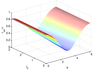
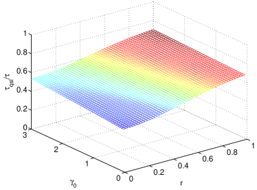
Figure 1: (Color online) The function of $\tau_{\text{qsl}}/\tau$ for damped Jaynes-Cummings model under squeezed environment. Panel (a), the ratio $\tau_{\text{qsl}}/\tau$ is varied along with the phase parameter $\theta$ and coupling strength $\gamma_{0}$. The squeezed parameter is chosen as $r=0.5$. Panel (b), it shows the variation of $\tau_{\text{qsl}}/\tau$ along with the squeezed parameter $r$ and coupling strength $\gamma_{0}$. The phase parameter is chosen as $\theta=0.5\pi$. In both panels, the spectral width is set as $\lambda=1$ (in units of $\omega_{0}$) and the actual driving time is chosen as $\tau=1$.

In Fig. 1, the behavior of ratio $\tau_{\text{qsl}}/\tau$ with squeezed environment parameters $r$ and $\theta$ are shown, respectively. In both panels, the environment spectral width is set as $\lambda=1$ (in units of $\omega_{0}$) and the actual driving time is chosen as $\tau=1$. In Panel (a), it is shown that the variation of quantum speed limit time along with the coupling strength $\gamma_{0}$ and phase parameter $\theta$. The squeezed parameter is chosen as $r=0.5$ and the quantum speed limit time shows symmetry about the phase parameter value $\theta=\pi$. The ML-type quantum speed limit time (7) is only comprised of the phase parameter $\theta$ with form $e^{i\theta}$ and its complex conjugate, so it presents periodic characteristics, obviously. When other parameters are fixed, the maximum of quantum speed limit time is located at $\theta=0$. It indicates that the appropriate phases parameter $\theta$ can accelerate the evolution of quantum states under squeezed environment.

Without loss of generality, the phase parameter is chosen as $\theta=0.5\pi$ in Panel (b), and the variation of quantum speed limit time along with the coupling strength $\gamma_{0}$ and squeezed parameter $r$ are demonstrated. The quantum speed limit time will become larger along with the increasing of squeezed parameter $r$. According to Eq. (7), a possible explanation is that the average evolution velocity of quantum system, i.e., $\Lambda_{\tau}^{\text{op}}$, will become slower when the squeezed parameter is increased, so the bound of quantum speed limit will be tight under squeezed environment.

Even though without Markovian approximation used in non-perturbative master equation (2), the variation of environment coupling strength $\gamma_{0}$ does not reflect the phenomenon of non-Markovianity for open quantum systems Breuer07 ; Breuer16 . It maybe caused by different methods to deal with the master equation. However, the quantum speed limit time will be larger along with the coupling strength $\gamma_{0}$ increasing, which is distinguished with the result in Ref. Deffner13 even when the squeezing effect is vanished.

IV The quantum speed limit for dephasing model

In this section, we will consider another pedagogical model, the dephasing model, and assume the environment interacting with quantum system is squeezed vacuum state, the total Hamiltonian of quantum system and environment is $H=\frac{1}{2}\omega_{0}\sigma_{z}+\sum_{k}\omega_{k}b_{k}^{{\dagger}}b_{k}+\sum_{k}g_{k}\sigma_{z}(b_{k}+k^{{\dagger}})$.

The initial quantum state is also assumed as maximal coherent state $|\psi_{0}\rangle=\frac{1}{\sqrt{2}}(|0\rangle+|1\rangle)$, and the evolved state is

$$\rho(t)=\left(\begin{array}[]{cc}\frac{1}{2}&\frac{1}{2}e^{-\gamma(t)}\\ \frac{1}{2}e^{-\gamma(t)}&\frac{1}{2}\\ \end{array}\right),$$ (10)

where the dephasing factor $\gamma(t)$ is defined by $\gamma(t)=\int d\omega J(\omega)\frac{1-\cos(\omega t)}{\omega^{2}}[\cosh(2r)-\cos(\omega t-\theta)\sinh(2r)]$. Without loss of generality, the structure of environment is Ohmic-like spectrum with soft cutoff

$$J(\omega)=\eta\frac{\omega^{s}}{\omega_{\text{c}}^{s-1}}\exp(-\frac{\omega}{\omega_{\text{c}}}),$$ (11)

where $\eta$ is the coupling parameter, the cutoff frequency $\omega_{\text{c}}$ is unity, and $s$ determines the type of environment, i.e., sub-Ohmic environment($s<1$), Ohmic environment ($s=1$), and super-Ohmic environment ($s>1$), respectively. The dephasing factor $\gamma(t)$ in Eq. (10) can be given analytically Wu17

$$\gamma(t)= \frac{\eta}{4}\Gamma(s-1)\{2\cosh(2r)[2-(1+it)^{1-s}-(1-it)^{1-s}]$$

$$+e^{-i\theta}\sinh(2r)[1-2(1-it)^{1-s}+(1-2it)^{1-s}]$$

$$+e^{i\theta}\sinh(2r)[1-2(1+it)^{1-s}+(1+2it)^{1-s}]\}.$$ (12)

The ML-type quantum speed limit time based on operator norm for dephasing model under squeezed environment can be given as following

$$\tau_{\text{qsl}}=\frac{\sin^{2}\mathcal{L}(\rho_{0},\rho_{\tau})}{\frac{1}{\tau}\int_{0}^{\tau}dt\|L_{t}(\rho_{t})\|_{\text{op}}},$$ (13)

where, $\sin^{2}\mathcal{L}(\rho_{0},\rho_{\tau})=\frac{1}{2}(1-e^{-\gamma(t)})$, and $\|L_{t}(\rho_{t})\|_{\text{op}}=\frac{1}{2}|\gamma^{\prime}(t)e^{-\gamma(t)}|$ with the dephasing rate

$$\gamma^{\prime}(t)= \frac{i\eta}{2}\Gamma(s)\{\cosh(2r)[(1+it)^{-s}-(1-it)^{-s}]$$

$$+e^{-i\theta}\sinh(2r)[(1-2it)^{-s}-(1-it)^{-s}]$$

$$+e^{i\theta}\sinh(2r)[(1+it)^{-s}-(1+2it)^{-s}]\}.$$ (14)

The quantum speed limit time for dephasing model under squeezed reservoir (13) is only determined by the dephasing rate $\gamma^{\prime}(t)$, and it shows acceleration features when the dephasing rate $\gamma^{\prime}(t)$ is negative, which is similar to the result in Ref. Wu15 . The sign of dephasing rate $\gamma^{\prime}(t)$ is depicted in Fig. 2, the squeezed parameter is chosen as $r=1$ and the driven time is chosen as $\tau=3$. The region of purple means that the value of $\gamma^{\prime}(t)$ is positive, while the white region means the corresponding negative range. Different to Ref. Wu15 , the boundary that the dephasing rate $\gamma^{\prime}(t)=0$ is a curve related to the squeezed parameters $r$ and $\theta$ in Fig. 2. The evolution of quantum system can be accelerated in the white region. Especially, the quantum speed limit bound under vacuum reservoir does not show speedup phenomena when $s\lesssim 2.5$ in Ref. Wu15 . Under the squeezed environment, this restricted condition can be broken when choosing appropriate squeezed environment parameters.

Figure 2: (Color online) The sign of dephasing rate $\gamma^{\prime}(t)$ in Eq. (14). The purple region means $\gamma^{\prime}(t)>0$ and the white region is $\gamma^{\prime}(t)<0$. The horizontal axis is Ohmic spectrum parameter $s$ and the vertical axis is phase parameter $\theta$. The squeezed parameter $r$ is set as $1$, and the actual driven time is chosen as $\tau=3$.

V Discussion and conclusion

We have investigated the quantum speed limit for open quantum system under squeezed environment. Two typical models, i.e., the damped Jaynes-Cummings model and the dephasing model, are considered, and the initial states are chosen as maximal coherent state for both models. For the damped Jaynes-Cummings model, the quantum speed limit time is larger along with the squeezed parameter $r$ increasing and shows symmetry about the phase parameter $\theta$. While, for the dephasing model, the quantum speed limit time is determined by the dephasing rate $\gamma^{\prime}(t)$ and the acceleration boundary that interacting with vacuum reservoir can be broken under the squeezed reservoir for appropriate squeezed parameters. We expect that our research has contribution to understand the evolution of quantum states in squeezed environments.

References

- (1) Mandelstam L and Tamm I, 1945 J. Phys. (Moscow) 9, 249.
- (2) Margolus N and Levitin L B, 1998 Phys. D (Amsterdam, Neth.) 120, 188.
- (3) Anandan J and Aharonov Y, 1990 Phys. Rev. Lett. 65, 1697.
- (4) Fleming G N, 1973 Nuovo Cimento 16, 232.
- (5) Bhattacharyya K, 1983 J. Phys. A 16, 2993.
- (6) Vaidman L, 1992 Am. J. Phys. 60, 182.
- (7) Giovannetti V, Lloyd S, and Maccone L, 2003 Phys. Rev. A 67, 052109.
- (8) Yung M H, 2006 Phys. Rev. A 74, 030303.
- (9) Jones P J, and Kok P, 2010 Phys. Rev. A 82, 022107.
- (10) Giovannetti V, Lloyd S, and Maccone L, 2012 Phys. Rev. Lett. 108, 260405.
- (11) Hegerfeldt G C, 2013 111, 260501.
- (12) Campaioli F, Pollock F A, Binder F C, and Modi K, 2018 Phys. Rev. Lett. 120, 060409.
- (13) Breuer H P and Petruccione F. 2007 The theory of open quantum systems. Oxford University Press, New York.
- (14) Breuer H P, Laine E M, Piilo J, and Vacchini B, 2016 Rev. Mod. Phys. 88, 021002.
- (15) Taddei M M, Escher B M, Davidovich L, and de Matos Filho R L, 2013 Phys. Rev. Lett. 110, 050402.
- (16) del Campo A, Egusquiza I L, Plenio M B, and Huelga S F, 2013 Phys. Rev. Lett. 110, 050403.
- (17) Deffner S and Lutz E, 2013 Phys. Rev. Lett. 111, 010402.
- (18) Xu Z Y, Luo S, Yang W L, Liu C, and Zhu S, 2014 Phys. Rev. A 89, 012307.
- (19) Zhang Y J, Han, Xia Y J, Cao J P, and Fan H, Sci. Rep. 4, 4890 (2014).
- (20) Wu S X, Zhang Y, Yu C S, and Song H S, 2015 J. Phys. A: Math. Theor. 48, 045301.
- (21) Liu C, Xu Z Y, and Zhu S, 2015 Phys. Rev. A 91, 022102.
- (22) Sun Z, Liu J, Ma J, and Wang X, 2015 Sci. Rep. 5, 8444.
- (23) Zhang Y J, Han W, Xia Y J, Cao J P, and Fan H, 2015 Phys. Rev. A 91, 032112.
- (24) Liu H B, Yang W L, An J H, and Xu Z Y, 2016 Phys. Rev. A 93, 020105.
- (25) Wei Y B, Zou J, Wang Z M, Shao B, and Li H, 2016 Phys. Lett. A 380, 397.
- (26) Song Y J, Kuang L M, and Tan Q S, 2016 Quantum Inf. Process. 15, 2325.
- (27) Cai X and Zheng Y, 2017 Phys. Rev. A 95, 052104.
- (28) Zhang L, Sun Y, and Luo S, 2018 Phys. Lett. A 382, 2599.
- (29) Wu S X, and Yu C S, 2018 Phys. Rev. A 98, 042132.
- (30) Xu K, Zhang G F, and Liu W M, 2019 Phys. Rev. A 100, 052305.
- (31) Wu S X, and Yu C S, 2020 Sci. Rep. 10, 5500.
- (32) Lu X, Zhang Y J, and Xia Y J, 2021 Chin. Phys. B 30, 020301.
- (33) Pires D P, Cianciaruso M, Céleri L C, Adesso G, and Soares-Pinto D O, 2016 Phys. Rev. X 6, 021031.
- (34) Marvian I, Spekkens R W, and Zanardi P, 2016 Phys. Rev. A 93, 052331.
- (35) Campbell S, and Deffner S, 2017 Phys. Rev. Lett. 118, 100601.
- (36) Xu Z Y, You W L, Dong Y L, Zhang C, and Yang W L, 2018 Phys. Rev. A 97, 032115.
- (37) Brody D C, and Longstaff B, 2019 Phys. Rev. Res. 1, 033127.
- (38) Bukov M, Sels D, and Polkovnikov A, 2019 Phys. Rev. X 9, 011034.
- (39) Fogarty T, Deffner S, Busch T, and Campbell S, 2020 Phys. Rev. Lett. 124, 110601.
- (40) Xu T N, Li J, Busch T, Chen X, and Fogarty T, 2020 Phys. Rev. Res. 2, 023125.
- (41) Suzuki K, and Takahashi K, 2020 Phys. Rev. Res. 2, 032016.
- (42) Sun S, and Zheng Y, 2019 Phys. Rev. Lett. 123, 180403.
- (43) Cimmarusti A D, Yan Z, Patterson B D, Corcos L P, Orozco L A, and Deffner S, 2015 Phys. Rev. Lett. 114, 233602.
- (44) Frey M R, 2016 Quantum Inf. Process. 15, 3919.
- (45) Deffner S, and Campbell S, 2017 J. Phys. A: Math. Theor. 50, 453001.
- (46) Deffner S, 2017 New J. Phys. 19, 103018.
- (47) Shiraishi N, Funo K, and Saito K, 2018 Phys. Rev. Lett. 121, 070601.
- (48) Okuyama M, and Ohzeki M, 2018 Phys. Rev. Lett. 120, 070402.
- (49) Shanahan B, Chenu A, Margolus N, and del Campo A, 2018 Phys. Rev. Lett. 120, 070401.
- (50) Nicholson S B, García-Pintos L P, del Campo A, and Green J R, 2020 Nature Phys. 16, 1211.
- (51) Wu S X, and Yu C S, 2020 Chin. Phys. B 29, 050302.
- (52) Hu X, Sun S, and Zheng Y, 2020 Phys. Rev. A 101, 042107.
- (53) Slusher R E, Hollberg L W, Yurke B, Mertz J C, and Valley J F, 1985 Phys. Rev. Lett. 55, 2409.
- (54) Wu L A, Kimble H J, Hall J L, and Wu H, 1986 Phys. Rev. Lett. 57, 2520.
- (55) Scully M O, and Zubairy M S, 1997 Quantum Optics, Cambridge University Press, Cambridge.
- (56) Caves C M, 1981 Phys. Rev. D 23, 1693.
- (57) Vahlbruch H, Khalaidovski A, Lastzka N, Gräf C, Danzmann K, and Schnabel R, Class. 2010 Quantum Grav. 27, 084027.
- (58) Wu S X, Yu C S, and Song H S, 2015 Phys. Lett. A 379, 1228.
- (59) Ishizaki A, and Tanimura Y, 2008 Chem. Phys. 347, 185.
- (60) Wang F Q, Zhang Z M, and Liang R S, 2009 Chin. Phys. B 18, 0597.
- (61) Wu S X, and Yu C S, Int. J. Theor. Phys. 56, 1198 (2017).