Improving Adversarial Robustness for Free with Snapshot Ensemble

Abstract

Adversarial training, as one of the few certified defenses against adversarial attacks, can be quite complicated and time-consuming, while the results might not be robust enough. To address the issue of lack of robustness, ensemble methods were proposed, aiming to get the final output by weighting the selected results from repeatedly trained processes. It is proved to be very useful in achieving robust and accurate results, but the computational and memory costs are even higher. Snapshot ensemble, a new ensemble method that combines several local minima in a single training process to make the final prediction, was proposed recently, which reduces the time spent on training multiple networks and the memory to store the results. Based on the snapshot ensemble, we present a new method that is easier to implement: unlike original snapshot ensemble that seeks for local minima, our snapshot ensemble focuses on the last few iterations of a training and stores the sets of parameters from them. Our algorithm is much simpler but the results are no less accurate than the original ones: based on different hyperparameters and datasets, our snapshot ensemble has shown a 5% to 30% increase in accuracy when compared to the traditional adversarial training.

1 Introduction

Deep learning has demonstrated considerable problem-solving abilities in broad computer engineering and visual analysis tasks since its emergence (Hinton et al., 2006), accompanied by long-term discussions of model performances of clean examples in various examinations and experiments. In recent years, however, discoveries on adversarial examples have lead to further evaluations on models’ vulnerable adversarial robustness and resulting security issues (Szegedy et al., 2013; Yuan et al., 2019; Goodfellow et al., 2014; Meng and Chen, 2017; Ma et al., 2018). What often happens to adversarial examples is that when images are slightly perturbed to fool classifiers, outputs will show a large fluctuation, further indicating the lack of robustness of models (Goodfellow et al., 2014).

Usually two methods are applied to process adversarial perturbations: the correct classification (Biggio et al., 2010; Guo et al., 2017; Moosavi-Dezfooli et al., 2017; Sankaranarayanan et al., 2018) and the selection of unperturbed images (Meng and Chen, 2017; Xu et al., 2017; Athalye et al., 2018a). The former relies on robust classifiers to make correct predictions on all the images, benign or adversarial, while the latter detects and filters the unperturbed images from adversarial examples, only on which it predicts. In particular, as the backbone of the correct classification, the adversarial training has been proved effective in numerous deep learning models (Goodfellow et al., 2014; Kurakin et al., 2016; Huang et al., 2015; Shrivastava et al., 2017; Tramèr et al., 2017), along with its apparently unstable, expensive, and time-consuming drawbacks (Madry et al., 2017; Sun et al., 2018). For stability issue, since slightly perturbed images can result in significant fluctuations in the outputs, there exist large variances within and between trials. Furthermore, for the computational complexity, the running time is usually three to thirty times that of the non-robust networks (Shafahi et al., 2019). This is mainly due to the time-consuming generation of adversarial examples which alone requires an optimization procedure, e.g. via fast gradient sign method (FGSM) (Goodfellow et al., 2014), projected gradient descent (PGD) (Goodfellow et al., 2014; Madry et al., 2017; Kurakin et al., 2016), One Pixel attack (Su et al., 2019), CW attack (Carlini and Wagner, 2016), or DeepFool (Moosavi-Dezfooli et al., 2015).

In the meanwhile, due to such defects of adversarial training, alternative methods have been proposed to improve its performances or to replace it. The Adversarial Robustness based Adaptive Label Smoothing (AR-AdaLS) proposed by Qin et al. (2020) aims to improve the smoothness of adversarial robustness in order to solve the instability: by training the model to distinguish the training data of varied adversarial robustness and by giving different supervision to the training data, their methods promotes label smoothing (Szegedy et al., 2013) and leads to better calibration and stability. Jakubovitz and Giryes (2018) and Hoffman et al. (2019) studied Jacobian regularization to regularize the training loss after the regular training, aiming to provide another way of enhancing robustness other than adversarial training. Mopuri et al. (2018), inspired by the architecture of GANs, attempted to capture the distribution of adversarial perturbation; their method exhibited extraordinary fooling rates, variety, and cross model generalizability.

There has been very few certified defenses (Lecuyer et al., 2019; Goodfellow et al., 2014; Cohen et al., 2019; Weng et al., 2018; Wong and Kolter, 2018) that are both applicable and functional in large scale problems such as ImageSet in recent years however, making adversarial training still remain the most trusted defense (Shafahi et al., 2019). Yet its troublesome features and the lack of outstanding performances on complex datasets make general tasks time-consuming, and large tasks almost unprocessable under ordinary circumstances, thus urging the need of finding other fast and for free methods that would raise adversarial robustness to the same level.

Contributions

Instead of improving performances of adversarial training, we study a training algorithm in which images are not perturbed in the dataset (either randomly as in certified robustness or adversarially as in adversarial training). The algorithm, while keeping the time spent on robust training almost equal to the non-robust ones, also produces robust models. Instead of perturbing the dataset, we apply the Snapshot Ensemble (Huang et al., 2017a; Smith, 2017; Loshchilov and Hutter, 2016) along the training process to store multiple historical weights so as to defend against adversarial attacks such as FGSM or PGD, in a Bayesian Neural Network (Blundell et al., 2015; Kingma et al., 2015; Ru et al., 2019; Zhang et al., 2021) manner. The proposed method produces results as fast as the non-robust networks, with only a few seconds difference when trained on CIFAR-10 (Krizhevsky et al., 2009) and MNIST (LeCun, 1998) datasets. The accuracy after attacks (i.e. the robust accuracy) with the ensemble during training is shown to be 5% to 30% better than the accuracy with regular training, depending on the dataset and perturbation magnitude $\epsilon$.

2 Background Knowledge

Adversarial Examples & Robustness

As previously introduced, the adversarial examples are the perturbed images or samples to fool the classifier in order to generate inaccurate outputs. Usually, the adversarial examples are defined within a range or perturbation set, for example, $l_{2}$ or $l_{\infty}$ spaces with a radius $\epsilon$. Here $\epsilon$ is also known as the perturbation magnitude. Therefore the adversarial example is

$$x+\delta^{*}\text{ where }\delta^{*}=\text{argmax}_{\delta}(\ell(f_{\theta}(x+\delta),y)\text{ s.t. }\|\delta\|_{p}\leq\epsilon$$ (1)

in which $\ell$ is the loss function, $f$ is the neural network governed by its parameters $\theta$, $x$ is the input sample, $y$ is the corresponding label and $\delta$ is the perturbation.

From the viewpoint of adversarial examples, we say a model is adversarially robust if a small perturbation $\delta$ does not change the output:

$$f_{\theta}(x+\delta)=f_{\theta}(x)$$ (2)

Numerous speculative hypotheses such as insufficient model averaging and regularizing had been proposed to address the causes of the existence of adversarial examples and model vulnerability before Goodfellow et al. (2014) found the determinate factor of the local linearity property of deep neural networks that even when non-linear activation functions are used, most of the training are manually operated in linear regions (Pascanu et al., 2013).

Adversarial Attack

Adversarial attack is a growing threat in the world of machine learning and deep learning, especially in applied fields such as computer vision and natural language processing. Based on the knowledge and goals of attackers, white-box and black-box attacks (Nidhra and Dondeti, 2012; Beizer, 1995) are commonly implemented to fulfill targeted (Szegedy et al., 2013) or non-targeted goals (Moosavi-Dezfooli et al., 2017; Athalye et al., 2018b). The aim of attackers is to insert a least amount of perturbation to the input to obtain desired misclassification (Huang et al., 2017b). An adversarial attack is, therefore, an optimization procedure to solve the constrained maximization problem (1).

Perturbation sets are what determine the constraints of the maximization problem (1), e.g. $l_{p}$ space such that:

$$\left\|\delta\right\|_{p}=\sqrt[p]{\sum_{i=1}^{k}\left|\delta_{i}\right|^{p}}\leq\epsilon$$ (3)

Among the $l_{p}$ spaces, $l_{0}$ (the number of non-zero elements in the vector), $l_{2}$, and $l_{\infty}$ are three commonly used norms in adversarial attacks, i.e.

$$\left\|\delta\right\|_{0}=\#\left(i\mid\delta_{i}\neq 0\right)\leq\epsilon,\quad\left\|\delta\right\|_{2}=\sqrt{\sum_{i=1}^{k}\left|\delta_{i}\right|^{2}}\leq\epsilon,\quad\left\|\delta\right\|_{\infty}=\max_{i}\left(\left|\delta_{i}\right|\right)\leq\epsilon$$ (4)

To $\textup{maximize}_{\left\|\delta\right\|_{p}\leq\epsilon}\ell(f_{\theta}(x+\delta),y)$, one usually performs a standard gradient ascent method over $\delta$, followed by a projection to ensure $\|\delta\|_{p}\leq\epsilon$. Many adversarial attack methods have been proposed. Here, we list and experiment on some prevalent attack methods:

• $l_{0}$ attack: OnePixel (Su et al., 2019), SparseFool (Modas et al., 2019)

• $l_{2}$ attack: Projected Gradient Descent-$l_{2}$ (PGDL2) (Goodfellow et al., 2014; Madry et al., 2017), DeepFool (Moosavi-Dezfooli et al., 2015), CW attack (Carlini and Wagner, 2016), AutoAttack-$l_{2}$ (Wong et al., 2020)

• $l_{\infty}$ attack: Fast Gradient Sign Method (FGSM) (Goodfellow et al., 2014), Projected Gradient Descent (PGD) (Goodfellow et al., 2014; Madry et al., 2017), AutoAttack-$l_{\infty}$ (Wong et al., 2020)

FGSM

As one of the earliest and most popular adversarial attacks described by Goodfellow et al. (2014), Fast Gradient Sign Method (FGSM) serves as a baseline attack in our training. As notified previously, to optimize the parameter in trained models is to maximize the loss function over $\delta$. We can increase the loss by moving constantly in the direction of the gradient by some step size (Goodfellow et al., 2014; Wiyatno et al., 2019), but because FGSM is a $l_{\infty}$ attack, the magnitude of gradients is restricted within the square threshold of $l_{\infty}$, so the direction is the only thing we need to care about. For gradients that exceed the threshold, we clip them back to the exact extrema of the perturbation set $\left[-\epsilon,\epsilon\right]$; for those within the threshold, because there are only two directions $+$ or $-$, we only need to adjust them also to the boundaries $\pm\epsilon$ accordingly to maximize the loss. Simply speaking, by taking the sign of the gradient, we obtain the optimal max-norm perturbation to be either $-\epsilon$ or $\epsilon$

$$\delta^{*}=\epsilon\cdot\mathrm{sign}(\nabla_{\delta}\ell(f_{\theta}(x+\delta),y))$$ (5)

PGD

Projected Gradient Descent (PGD) is the more careful iteration of updates of FGSM with smaller step sizes

$$\delta_{t+1}=\mathcal{P}(\delta_{t}+\alpha\nabla_{\delta_{t}}\ell(f_{\theta}(x+\delta_{t}),y))$$ (6)

where $\mathcal{P}$ stands for the projection back to the $l_{\infty}$ norm (clipping or truncating within range $\left[-\epsilon,\epsilon\right]$) (Wiyatno et al., 2019; Madry et al., 2017). Note that PGD also has the form of $l_{2}$ version and it is the workhorse in adversarial attack nowadays.

Adversarial Training

Normally when training a non-robust classifier we want to optimize the parameter $\theta$ by minimizing the average loss

$$\mathop{\textup{minimize}}\limits_{\theta}\frac{1}{n}\sum_{i=1}^{n}\ell(f_{\theta}(x_{i}),y_{i})$$ (7)

where {$x_{i}\in\mathcal{X},y_{i}\in\mathcal{Y}\},i=1,...,n$, and $f_{\theta}$ the function that $\mathcal{X}\to\mathcal{Y}$. In adversarial training, we instead want to optimize $\theta$ by the minimax problem:

$$\mathop{\textup{minimize}}\limits_{\theta}\frac{1}{n}\sum_{i=1}^{n}\mathop{\textup{maximize}}\limits_{\delta:\|\delta\|_{p}\leq\ \epsilon}\ell(f_{\theta}(x_{i}+\delta),y_{i})$$ (8)

Algorithically speaking, at each iteration, one needs to solve the inner constrained maximization, e.g. by PGD or FGSM, and then the outer minimizaiton, e.g. by standard SGD or Adam.

Algorithm 1 Adversarial Training with FGSM

1:Input: Training Sample $\mathcal{X}$; Neural Network $f_{\theta}$; Perturbation bound $\epsilon$; Learning Rate $\eta$; Total Epoch $T$;

2:Process:

3:Initialize $\theta$ randomly and set $\delta\leftarrow 0$

4:for epoch = $1,\cdots,T$ do

5:     for minibatch $B\subset\mathcal{X}$ do

6:         $g_{adv}=\nabla_{\delta}\ell(f_{\theta}(x+\delta),y)$

7:         Maximization: Update $\delta$ by $\delta+\epsilon\cdot$sign($g_{adv}$) and then clip to $\left[-\epsilon,\epsilon\right]$

8:         $g_{\theta}=\nabla_{\theta}\ell(f_{\theta}(x+\delta),y)$ where x, y $\in$ B

9:         Minimization: Update $\theta$ by $\theta-\eta\cdot g_{\theta}$

10:     end for

11:end for

Snapshot Ensemble

Regular training, or as Gawlikowski et al. (2021) refer to as deterministic methods, is an one-to-one process that one input after classification predicts one output, but it is not sufficient to produce accurate and robust results. To improve on this, the ensemble methods and the Bayesian Neural Networks (BNN) were proposed, both at the cost of higher computation and memory cost (Zhou, 2021). Recently, a new method of ensemble learning called snapshot ensemble learning (SEL) was proposed (Huang et al., 2017a). Unlike Stochastic Gradient Descent (SGD), which avoids saddle points and local minima (Bottou, 2010; Dauphin et al., 2014), SEL stores and ensembles the local minima to improve model performances: by dividing the training process into multiple cycles, the small learning rate encourages the model to converge towards the local minima, and then SEL combines these local minima (Huang et al., 2017a; Wen et al., 2019).

In this work, we propose a new ensemble similar to SEL in spirit, i.e. collecting and ensembling network parameters along the single training procedure. However, our ensemble does not require local minima and treats the parameters at each iteration as a random draw from the limiting distribution of parameters, which is detailed in Section 3.

• Regular ensemble: initialize $M$ neural networks with parameters $\theta_{1}(0),\cdots,\theta_{M}(0)$ and train separately to get $\theta_{1}(t),\cdots,\theta_{M}(t)$ at the $t$-th iteration; the final prediction is $\sum_{i}f_{\theta_{i}(t)}(x)$.

• Original snapshot ensemble: initialize 1 neural network with $\theta_{1}(0)$ and use $M$ local minima $\theta_{1}(t_{j})$ where $j\in[M]$ during the training process; the final prediction is $\sum_{j}f_{\theta_{1}(t_{j})}(x)$.

• Our snapshot ensemble: initialize 1 neural network with $\theta_{1}(0)$ and use the last $M$ iterations in the epoch $\theta_{1}(t-M+1),\cdots,\theta_{1}(t)$; the final prediction is $\sum_{i}f_{\theta_{1}(t-i+1)}(x)$.

3 Snapshot Ensemble Improves Adversarial Robustness

Algorithm 2 Our Snapshot Ensemble

1:Input: Dataset $\mathcal{D}=\left\{\left(x_{1},y_{1}\right),\cdots,\left(x_{n},y_{n}\right)\right\}$; network model $f$ with trainable parameters $\theta_{t}$; number of iterations $T$; number of copies $M$; optimizer $A$

2:for $t=1,\cdots,T$ do

3:     $D_{t}$ = sample(Bootstrap) from $\mathcal{D}$ (Batch)

4:     $\theta_{t}=A(D_{t},\theta_{t-1},f)$

5:end for

6:Output: $f\left(x\right)$ = $\sum_{k=T-M+1}^{T}{f}\left(x;\theta_{k}\right)$

Instead of training multiple networks (like regular ensemble method), both original SEL and ours only need to train a single network, therefore saving the computational complexity by $M$ times. However, both SEL needs to store $M$ sets of historical parameters, hence requiring higher memory cost than the regular ensemble.

We further distinguish our SEL with the traditional SEL. The original SEL seeks multiple local minima via the so-called cosine annealing learning rate (Loshchilov and Hutter, 2016, 2017) that adjusts the magnitude of learning rate during training. As the epoch increases, cosine annealing learning rate first decreases and then rises rapidly at the end of each cosine cycle to escape from the local minima (Huang et al., 2017a). The process is then repeated several times until all the epochs are finished. By recording the local minima, we can use a combination strategy (voting, averaging, second-level learning, etc.) to compute the weighted result that exceeds the original accuracy rate and shows an steady increase at all the recorded spots when compared with the base model (Brownlee, 2018; Huang et al., 2017a; Izmailov et al., 2018; Loshchilov and Hutter, 2017).

Our snapshot ensemble, however, does not concern the cosine annealing and local minima. Unlike the regular snapshot ensemble that uses a complicated process to collect sample points at local minima (Loshchilov and Hutter, 2016, 2017; Huang et al., 2017a) or the BNN that regards the weight as a Gaussian distribution with a mean and a variance and optimizes them for each weights (Anzai, 2012; Gawlikowski et al., 2021), we are looking for a simpler snapshot ensemble method that extracts weights from the last few iterations and compute the weighted output accordingly. Through experiments on different datasets and attack methods, our SEL consistently shows significant better robust accuracy, with 5% to 30%increase from the regular accuracy.

4 Experiments

Our experiments are implemented with two commonly used datasets: MNIST (LeCun, 1998) and CIFAR-10 (Krizhevsky et al., 2009). The MNIST set is a 28 $\times$ 28 grey scale dataset with 60000 training and 10000 testing figures of hand written numeric figure. The CIFAR-10 set consists of 6000 examples of 10 classes, with 50000 training figures and 10000 testing figures. Being the 3-channel (RGB) 32 $\times$ 32 pixels color dataset, CIFAR-10 contains objects in real world that have not only a higher level of noises but very diverse features and scales, making the CIFAR-10 set less resistant to adversarial attacks and tougher to reflect the performances of numerous models (Pang et al., 2019; Yin et al., 2019; Peck et al., 2017; Sen et al., 2020).

The optimizers I have chosen are Stochastic Gradient Descent (SGD), Heavy Ball (HB, i.e. SGD with a momentum), and Nesterov Accelerated Gradient (NAG), with more concentration on Heavy Ball. Gradient Descent (GD), as one of the oldest and the most prevalent optimizers, is a method that finds the minimum loss step by step. While GD takes in all the data in each step, SGD stochastically picks a single point and updates for the parameters. Every step of SGD is weaker than GD, but because it also takes less total steps with a faster pace, SGD saves a lot more time. Therefore, SGD has become the most welcomed optimizer for its simplicity and time-saving.

Heavy ball method is a modified form of gradient descent: in each step of gradient descent, the optimizer generates a momentum vector in the direction of this step and a given magnitude so that in the next step, this momentum is composed with the new gradient descent that nudges the new parameters in the magnitude and direction of the previous step (Ghadimi et al., 2015; Gadat et al., 2018; Sutskever et al., 2013; Saunders, 2018; Ruder, 2016; Botev et al., 2017). It is like the movement of a heavy ball in the real world: when the ball’s movement direction changes, it will be affected by the previous movement trend and will present a result slightly deviating from the expectation. Unlike SGD that stresses the global minimum and becomes invalid at local extrema or non-convex points, the momentum of heavy ball could bring the steps out from local extrema with no extra time spends, yet there have been less focuses on it since its proposal by Polyak in 1964. Therefore, we have chosen to do our experiments with more concentrations on heavy ball.

NAG is the smarter version of heavy ball, that is, it takes in two successive steps to decide the momentum. Through the intermediate point we can determine from the previous two steps what the momentum in the current step should be like and make a correction accordingly (Ruder, 2016; Saunders, 2018; Lin et al., 2019; Botev et al., 2017).

The neural network architecture for CIFAR-10 is taken from Pytorch tutorial, and that for MNIST is adapted by changing the second hidden layer from 400 to 256 units.

Some default hyperparameters: learning rate = 0.02; momentum = 0.9; snapshot = 20; epoch = 20; epsilons = [0.0, 0.01, 0.02, 0.03, 0.04]; weight decay = 0.0; alpha (PGD) = 0.02; steps (PGD) = 2; random start (PGD) = False. One or more of these hyperparameters are adjusted in different experiments accordingly; other hyperparameters, otherwise notified, are used as default in the experiments.

4.1 CIFAR-10

Different colors represent different attack magnitude $\epsilon$ of FGSM. Dashed line is our snapshot ensemble with four different snapshots. Solid line is regular training. Default number of snapshots is 10. Notice that when $\epsilon=0$, the accuracy is indeed the clean accuracy without suffering the attack.

4.1.1 Outer minimization optimizers

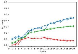
(a) SGD

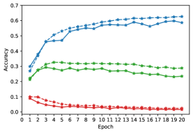
(b) NAG

(c) HB

Figure 1: Adversarial accuracy of neural networks on CIFAR-10 under FGSM, trained with different optimizers.

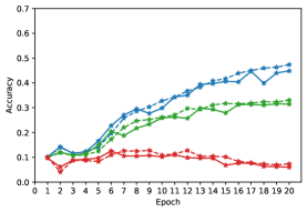
(a) SGD

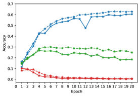
(b) NAG

(c) HB

Figure 2: Adversarial accuracy of neural networks on CIFAR-10 under PGD, trained with different optimizers.

From Figure 1 and Figure 2 we observe that, fixing an attack, the outer minimization optimizer does affect on the adversarial robustness of neural networks. For example, when attacked by FGSM or PGD with $\epsilon=0.01$, the neural network learned by SGD has around 30% accuracy, while momentum methods achieve around 20%. On the other hand, our snapshot ensemble improves much more on momentum methods (roughly 10%) than on SGD. In addition, different attacks seem to have small effects on the performance under various $\epsilon$.

4.1.2 Number of snapshots

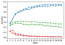
(a) 98 snapshots

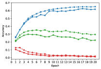
(b) 40 snapshots

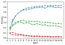
(c) 20 snapshots

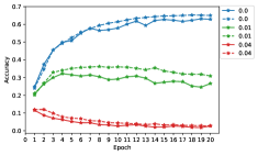
(d) 10 snapshots

Figure 3: Adversarial accuracy of neural networks on CIFAR-10 under FGSM, ensembled with different snapshots.

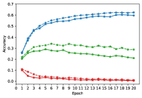
(a) 98 snapshots

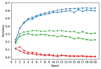
(b) 40 snapshots

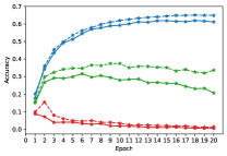
(c) 20 snapshots

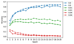
(d) 10 snapshots

Figure 4: Adversarial accuracy of neural networks on CIFAR-10 under PGD, ensembled with different snapshots.

From Figure 3 and Figure 4 we see that the number of snapshots has ignorable influence on the adversarial accuracy. Because more snapshots consume more time spent on ensembling (in other words, prediction time) and more memory to store the historical weights from past iterations, our experiments suggest that using a small number of snapshots is sufficient in practice.

4.1.3 Learning rate

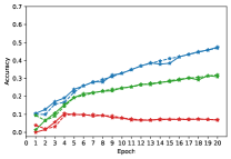
(a) 0.002 learning rate

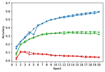
(b) 0.005 learning rate

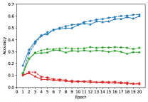
(c) 0.01 learning rate

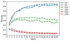
(d) 0.02 learning rate

Figure 5: Adversarial accuracy of neural networks on CIFAR-10 under FGSM, trained with different learning rates.

(a) 0.002 learning rate

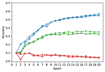
(b) 0.005 learning rate

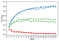
(c) 0.01 learning rate

(d) 0.02 learning rate

Figure 6: Adversarial accuracy of neural networks on CIFAR-10 under PGD, trained with different learning rates.

From Figure 5 and Figure 6 we can see that a higher learning rate corresponds to a higher adversarial accuracy. Especially, larger learning rate has a more significant effect on the performance of our snapshot ensemble. It is clear that a small magnitude of learning rate produces non-robust results, but an excessively large learning rate could have the same bad effect since the models may not converge.

4.1.4 Momentum coefficient

(a) 0.5 momentum

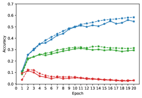
(b) 0.7 momentum

(c) 0.9 momentum

Figure 7: Adversarial accuracy of neural networks on CIFAR-10 under FGSM, trained with different momentums.

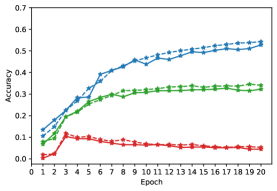
(a) 0.5 momentum

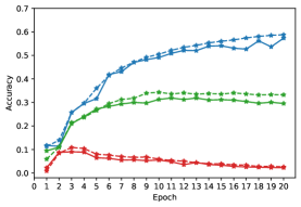
(b) 0.7 momentum

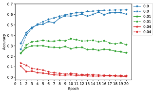
(c) 0.9 momentum

Figure 8: Adversarial accuracy of neural networks on CIFAR-10 under PGD, trained with different momentums.

From Figure 7 and Figure 8 we also observe that a higher momentum corresponds to a higher adversarial accuracy and again that higher momentum with our snapshot ensemble improves the performance more significantly.

4.2 MNIST

The above conclusions for the CIFAR-10 dataset are also applicable for the MNIST dataset, but due to the characteristics of the MNIST images, the adversarial robustness is very strong, and the graphically slight increases cannot be clearly displayed, we do not repeatedly show them here. You may find the section in more details in the appendix.

5 Conclusion

In summary, we propose a new adversarial training procedure that does not require any changes to the training but incorporates the ensemble method during iterations. Our method takes the same computational complexity as the traditional adversarial training and improves the accuracy consistently. In fact, our ensemble is similar to the snapshot ensemble, but easier to implement, since we stores sets of parameters from last iterations instead of the local minima.

At the core of our method is the randomness of stored parameters. It naturally begs the question of what types of noises are present and what are their effects. For example, using standard SGD or most gradient methods with minibatch, there exists the sampling noise which empirically improves the robust accuracy. In gradient methods like stochastic gradient Langevin dynamics, the noise is isotropic (independent of data) and may have different effects than the sampling noise. Another example could be the random data augmentation, especially in image tasks. Training (either regularly or adversarially) on such tasks involve the transformation noise into the process, leading to uncertain effect on robustness. It would be desirable to conduct further experiments on these various sources of noise and on larger scale of datasets.

Appendix A Neural Network Architectures

The neural network architectures for MNIST and CIFAR-10 datasets are as follows:

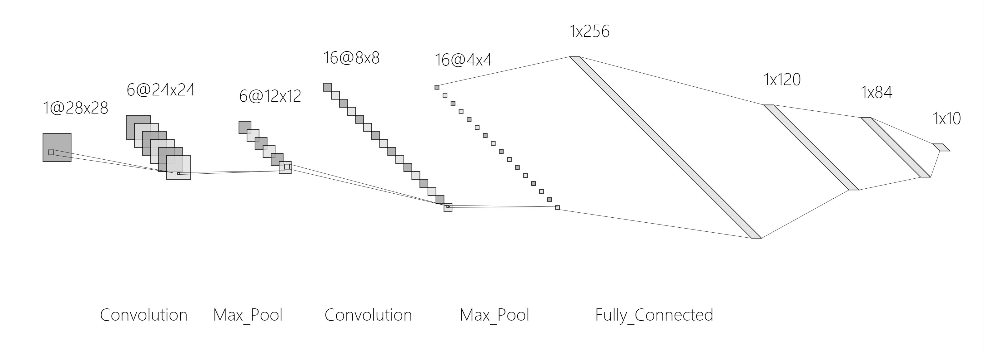
Figure 9: MNIST Neural Network Architecture

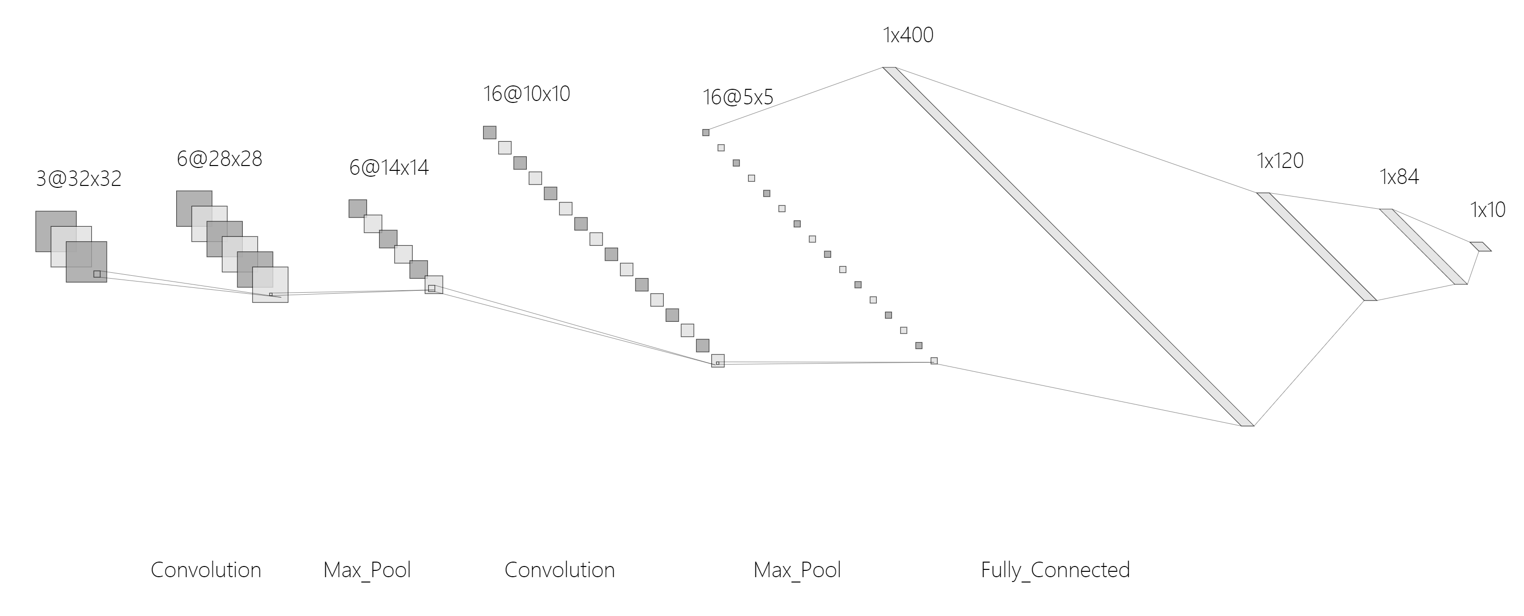
Figure 10: CIFAR-10 Neural Network Architecture

Appendix B MNIST

Due to MNIST’s extreme robustness, we have enlarged some graphs and have removed several beginning epochs from some of the graphs to amplify the differences.

B.0.1 Outer minimization optimizers

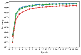
(a) SGD

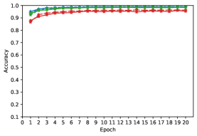
(b) NAG

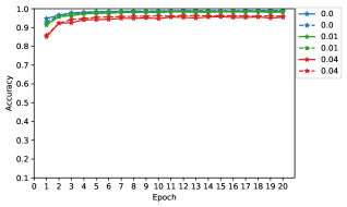
(c) HB

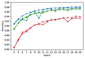
(d) SGD (zoomed in)

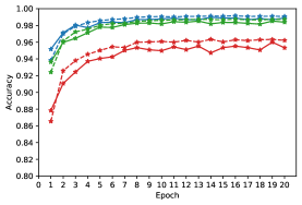
(e) NAG (zoomed in)

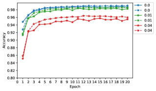
(f) HB (zoomed in)

Figure 11: Adversarial accuracy of neural networks on MNIST under FGSM, trained with different optimizers.

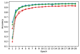
(a) SGD

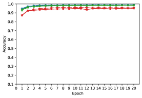
(b) NAG

(c) HB

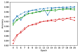
(d) SGD (zoomed in)

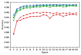
(e) NAG (zoomed in)

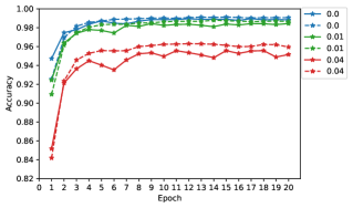
(f) HB (zoomed in)

Figure 12: Adversarial accuracy of neural networks on MNIST under PGD, trained with different optimizers.

From Figure 11 and Figure 12 we observe that, fixing the adversarial attack, the outer minimization optimizer does affect the adversarial robustness of neural networks. For example, when attacked by FGSM or PGD with $\epsilon=0.01$, the neural network learned by SGD, especially in the first two epochs, has a very low accuracy (from 18% to 93% at a slow growth rate) compared with the accuracy achieved by momentum methods, in which almost all the results are above 92% accuracy (except for the first epoch, which is still much greater than the 18% from the first epoch of SGD) and can be up to 96% accuracy. On the other hand, our snapshot ensemble improves much more on momentum methods (roughly 5%) than on SGD. In addition, different attacks seem to have small effects on the performance under varied $\epsilon$.

B.0.2 Number of snapshots

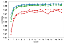
(a) 98 snapshots

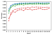
(b) 40 snapshots

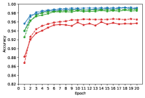
(c) 20 snapshots

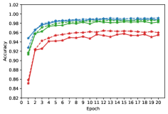
(d) 10 snapshots

Figure 13: Adversarial accuracy of neural networks on MNIST under FGSM, ensembled with different snapshots.

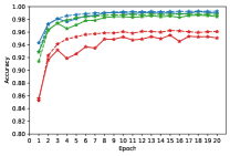
(a) 98 snapshots

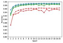
(b) 40 snapshots

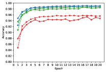
(c) 20 snapshots

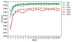
(d) 10 snapshots

Figure 14: Adversarial accuracy of neural networks on MNIST under PGD, ensembled with different snapshots.

From Figure 13 and Figure 14 we can see that the number of snapshots has the same ignorable influence on the adversarial accuracy in MNIST dataset. Because more snapshots consume more time spent on ensembling (in other words, prediction time) and more memory to store the historical weights from past iterations, our experiments suggest that using a small number of snapshots would be sufficient in practice.

B.0.3 Learning rate

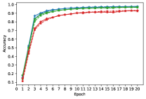
(a) 0.002 learning rate

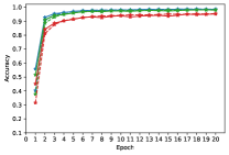
(b) 0.005 learning rate

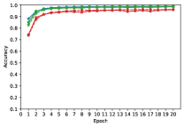
(c) 0.01 learning rate

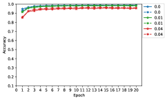
(d) 0.02 learning rate

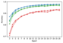
(e) 0.002 lr (zoomed in)

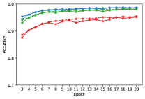
(f) 0.005 lr (zoomed in)

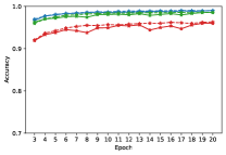
(g) 0.01 lr (zoomed in)

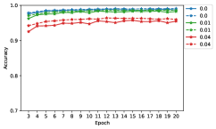
(h) 0.02 lr (zoomed in)

Figure 15: Adversarial accuracy of neural networks on MNIST under FGSM, trained with different learning rates.

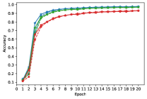
(a) 0.002 learning rate

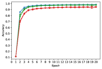
(b) 0.005 learning rate

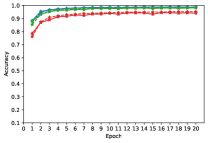
(c) 0.01 learning rate

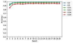
(d) 0.02 learning rate

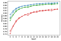
(e) 0.002 lr (zoomed in)

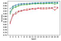
(f) 0.005 lr (zoomed in)

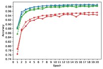
(g) 0.01 lr (zoomed in)

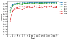
(h) 0.02 lr (zoomed in)

Figure 16: Adversarial accuracy of neural networks on MNIST under PGD, trained with different learning rates.

From Figure 15 and Figure 16 we can see that a larger learning rate corresponds to a higher adversarial accuracy and has a more significant effect on the performance of our snapshot ensemble especially. It is clear that a small magnitude of learning rate produces non-robust results, but an excessively large learning rate could have the same negative effects since the models may not converge.

B.0.4 Momentum coefficient

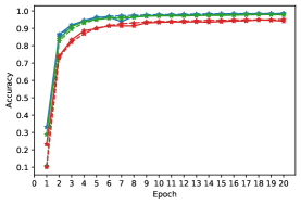
(a) 0.5 momentum

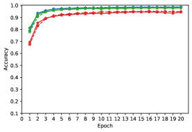
(b) 0.7 momentum

(c) 0.9 momentum

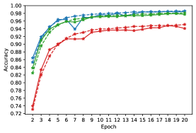
(d) 0.5 momentum (zoomed in)

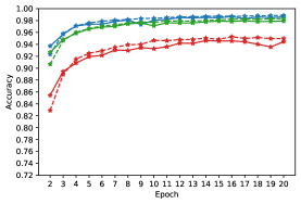
(e) 0.7 momentum (zoomed in)

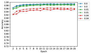
(f) 0.9 momentum (zoomed in)

Figure 17: Adversarial accuracy of neural networks on MNIST under FGSM, trained with different momentums.

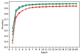
(a) 0.5 momentum

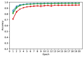
(b) 0.7 momentum

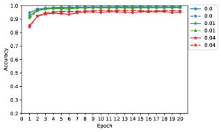
(c) 0.9 momentum

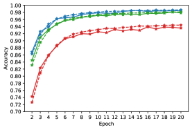
(d) 0.5 momentum (zoomed in)

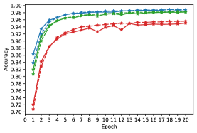
(e) 0.7 momentum (zoomed in)

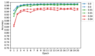
(f) 0.9 momentum (zoomed in)

Figure 18: Adversarial accuracy of neural networks on MNIST under PGD, trained with different momentums.

From Figure 17 and Figure 18 we can observe the same phenomenon that a higher momentum corresponds to a higher adversarial accuracy and again that higher momentum with our snapshot ensemble improves the performance more significantly.

References

- Hinton et al. [2006] Geoffrey E Hinton, Simon Osindero, and Yee-Whye Teh. A fast learning algorithm for deep belief nets. Neural computation, 18(7):1527–1554, 2006.
- Szegedy et al. [2013] Christian Szegedy, Wojciech Zaremba, Ilya Sutskever, Joan Bruna, Dumitru Erhan, Ian Goodfellow, and Rob Fergus. Intriguing properties of neural networks. arXiv preprint arXiv:1312.6199, 2013.
- Yuan et al. [2019] Xiaoyong Yuan, Pan He, Qile Zhu, and Xiaolin Li. Adversarial examples: Attacks and defenses for deep learning. IEEE transactions on neural networks and learning systems, 30(9):2805–2824, 2019.
- Goodfellow et al. [2014] Ian J Goodfellow, Jonathon Shlens, and Christian Szegedy. Explaining and harnessing adversarial examples. arXiv preprint arXiv:1412.6572, 2014.
- Meng and Chen [2017] Dongyu Meng and Hao Chen. Magnet: a two-pronged defense against adversarial examples. In Proceedings of the 2017 ACM SIGSAC conference on computer and communications security, pages 135–147, 2017.
- Ma et al. [2018] Xingjun Ma, Bo Li, Yisen Wang, Sarah M Erfani, Sudanthi Wijewickrema, Grant Schoenebeck, Dawn Song, Michael E Houle, and James Bailey. Characterizing adversarial subspaces using local intrinsic dimensionality. arXiv preprint arXiv:1801.02613, 2018.
- Biggio et al. [2010] Battista Biggio, Giorgio Fumera, and Fabio Roli. Multiple classifier systems for robust classifier design in adversarial environments. International Journal of Machine Learning and Cybernetics, 1(1-4):27–41, 2010.
- Guo et al. [2017] Chuan Guo, Geoff Pleiss, Yu Sun, and Kilian Q Weinberger. On calibration of modern neural networks. In International Conference on Machine Learning, pages 1321–1330. PMLR, 2017.
- Moosavi-Dezfooli et al. [2017] Seyed-Mohsen Moosavi-Dezfooli, Alhussein Fawzi, Omar Fawzi, and Pascal Frossard. Universal adversarial perturbations. In Proceedings of the IEEE conference on computer vision and pattern recognition, pages 1765–1773, 2017.
- Sankaranarayanan et al. [2018] Swami Sankaranarayanan, Arpit Jain, Rama Chellappa, and Ser Nam Lim. Regularizing deep networks using efficient layerwise adversarial training. In Thirty-Second AAAI Conference on Artificial Intelligence, 2018.
- Xu et al. [2017] Weilin Xu, David Evans, and Yanjun Qi. Feature squeezing: Detecting adversarial examples in deep neural networks. arXiv preprint arXiv:1704.01155, 2017.
- Athalye et al. [2018a] Anish Athalye, Nicholas Carlini, and David Wagner. Obfuscated gradients give a false sense of security: Circumventing defenses to adversarial examples. In International conference on machine learning, pages 274–283. PMLR, 2018a.
- Kurakin et al. [2016] Alexey Kurakin, Ian Goodfellow, and Samy Bengio. Adversarial machine learning at scale. arXiv preprint arXiv:1611.01236, 2016.
- Huang et al. [2015] Ruitong Huang, Bing Xu, Dale Schuurmans, and Csaba Szepesvári. Learning with a strong adversary. arXiv preprint arXiv:1511.03034, 2015.
- Shrivastava et al. [2017] Ashish Shrivastava, Tomas Pfister, Oncel Tuzel, Joshua Susskind, Wenda Wang, and Russell Webb. Learning from simulated and unsupervised images through adversarial training. In Proceedings of the IEEE conference on computer vision and pattern recognition, pages 2107–2116, 2017.
- Tramèr et al. [2017] Florian Tramèr, Alexey Kurakin, Nicolas Papernot, Ian Goodfellow, Dan Boneh, and Patrick McDaniel. Ensemble adversarial training: Attacks and defenses. arXiv preprint arXiv:1705.07204, 2017.
- Madry et al. [2017] Aleksander Madry, Aleksandar Makelov, Ludwig Schmidt, Dimitris Tsipras, and Adrian Vladu. Towards deep learning models resistant to adversarial attacks. arXiv preprint arXiv:1706.06083, 2017.
- Sun et al. [2018] Sining Sun, Ching-Feng Yeh, Mei-Yuh Hwang, Mari Ostendorf, and Lei Xie. Domain adversarial training for accented speech recognition. In 2018 IEEE International Conference on Acoustics, Speech and Signal Processing (ICASSP), pages 4854–4858. IEEE, 2018.
- Shafahi et al. [2019] Ali Shafahi, Mahyar Najibi, Amin Ghiasi, Zheng Xu, John Dickerson, Christoph Studer, Larry S Davis, Gavin Taylor, and Tom Goldstein. Adversarial training for free! arXiv preprint arXiv:1904.12843, 2019.
- Su et al. [2019] Jiawei Su, Danilo Vasconcellos Vargas, and Kouichi Sakurai. One pixel attack for fooling deep neural networks. IEEE Transactions on Evolutionary Computation, 23(5):828–841, 2019.
- Carlini and Wagner [2016] Nicholas Carlini and David A Wagner. Towards evaluating the robustness of neural networks. corr abs/1608.04644 (2016). arXiv preprint arXiv:1608.04644, 2016.
- Moosavi-Dezfooli et al. [2015] Seyed-Mohsen Moosavi-Dezfooli, Alhussein Fawzi, and Pascal Frossard. Deepfool: a simple and accurate method to fool deep neural networks. corr abs/1511.04599 (2015). arXiv preprint arXiv:1511.04599, 2015.
- Qin et al. [2020] Yao Qin, Xuezhi Wang, Alex Beutel, and Ed H Chi. Improving uncertainty estimates through the relationship with adversarial robustness. arXiv preprint arXiv:2006.16375, 2020.
- Jakubovitz and Giryes [2018] Daniel Jakubovitz and Raja Giryes. Improving dnn robustness to adversarial attacks using jacobian regularization. In Proceedings of the European Conference on Computer Vision (ECCV), pages 514–529, 2018.
- Hoffman et al. [2019] Judy Hoffman, Daniel A Roberts, and Sho Yaida. Robust learning with jacobian regularization. arXiv preprint arXiv:1908.02729, 2019.
- Mopuri et al. [2018] Konda Reddy Mopuri, Utkarsh Ojha, Utsav Garg, and R Venkatesh Babu. Nag: Network for adversary generation. In Proceedings of the IEEE Conference on Computer Vision and Pattern Recognition, pages 742–751, 2018.
- Lecuyer et al. [2019] Mathias Lecuyer, Vaggelis Atlidakis, Roxana Geambasu, Daniel Hsu, and Suman Jana. Certified robustness to adversarial examples with differential privacy. In 2019 IEEE Symposium on Security and Privacy (SP), pages 656–672. IEEE, 2019.
- Cohen et al. [2019] Jeremy Cohen, Elan Rosenfeld, and Zico Kolter. Certified adversarial robustness via randomized smoothing. In International Conference on Machine Learning, pages 1310–1320. PMLR, 2019.
- Weng et al. [2018] Lily Weng, Huan Zhang, Hongge Chen, Zhao Song, Cho-Jui Hsieh, Luca Daniel, Duane Boning, and Inderjit Dhillon. Towards fast computation of certified robustness for relu networks. In International Conference on Machine Learning, pages 5276–5285. PMLR, 2018.
- Wong and Kolter [2018] Eric Wong and Zico Kolter. Provable defenses against adversarial examples via the convex outer adversarial polytope. In International Conference on Machine Learning, pages 5286–5295. PMLR, 2018.
- Huang et al. [2017a] Gao Huang, Yixuan Li, Geoff Pleiss, Zhuang Liu, John E Hopcroft, and Kilian Q Weinberger. Snapshot ensembles: Train 1, get m for free. arXiv preprint arXiv:1704.00109, 2017a.
- Smith [2017] Leslie N Smith. Cyclical learning rates for training neural networks. In 2017 IEEE winter conference on applications of computer vision (WACV), pages 464–472. IEEE, 2017.
- Loshchilov and Hutter [2016] Ilya Loshchilov and Frank Hutter. Sgdr: Stochastic gradient descent with warm restarts. arXiv preprint arXiv:1608.03983, 2016.
- Blundell et al. [2015] Charles Blundell, Julien Cornebise, Koray Kavukcuoglu, and Daan Wierstra. Weight uncertainty in neural network. In International Conference on Machine Learning, pages 1613–1622. PMLR, 2015.
- Kingma et al. [2015] Durk P Kingma, Tim Salimans, and Max Welling. Variational dropout and the local reparameterization trick. Advances in neural information processing systems, 28:2575–2583, 2015.
- Ru et al. [2019] Binxin Ru, Adam Cobb, Arno Blaas, and Yarin Gal. Bayesopt adversarial attack. In International Conference on Learning Representations, 2019.
- Zhang et al. [2021] Qiyiwen Zhang, Zhiqi Bu, Kan Chen, and Qi Long. Differentially private bayesian neural networks on accuracy, privacy and reliability. arXiv preprint arXiv:2107.08461, 2021.
- Krizhevsky et al. [2009] Alex Krizhevsky, Geoffrey Hinton, et al. Learning multiple layers of features from tiny images. 2009.
- LeCun [1998] Yann LeCun. The mnist database of handwritten digits. http://yann. lecun. com/exdb/mnist/, 1998.
- Pascanu et al. [2013] Razvan Pascanu, Tomas Mikolov, and Yoshua Bengio. On the difficulty of training recurrent neural networks. In International conference on machine learning, pages 1310–1318. PMLR, 2013.
- Nidhra and Dondeti [2012] Srinivas Nidhra and Jagruthi Dondeti. Black box and white box testing techniques-a literature review. International Journal of Embedded Systems and Applications (IJESA), 2(2):29–50, 2012.
- Beizer [1995] Boris Beizer. Black-box testing: techniques for functional testing of software and systems. John Wiley & Sons, Inc., 1995.
- Athalye et al. [2018b] Anish Athalye, Logan Engstrom, Andrew Ilyas, and Kevin Kwok. Synthesizing robust adversarial examples. In International conference on machine learning, pages 284–293. PMLR, 2018b.
- Huang et al. [2017b] Sandy Huang, Nicolas Papernot, Ian Goodfellow, Yan Duan, and Pieter Abbeel. Adversarial attacks on neural network policies. arXiv preprint arXiv:1702.02284, 2017b.
- Modas et al. [2019] Apostolos Modas, Seyed-Mohsen Moosavi-Dezfooli, and Pascal Frossard. Sparsefool: a few pixels make a big difference. In Proceedings of the IEEE/CVF conference on computer vision and pattern recognition, pages 9087–9096, 2019.
- Wong et al. [2020] Eric Wong, Leslie Rice, and J Zico Kolter. Fast is better than free: Revisiting adversarial training. arXiv preprint arXiv:2001.03994, 2020.
- Wiyatno et al. [2019] Rey Reza Wiyatno, Anqi Xu, Ousmane Dia, and Archy de Berker. Adversarial examples in modern machine learning: A review. arXiv preprint arXiv:1911.05268, 2019.
- Gawlikowski et al. [2021] Jakob Gawlikowski, Cedrique Rovile Njieutcheu Tassi, Mohsin Ali, Jongseok Lee, Matthias Humt, Jianxiang Feng, Anna Kruspe, Rudolph Triebel, Peter Jung, Ribana Roscher, et al. A survey of uncertainty in deep neural networks. arXiv preprint arXiv:2107.03342, 2021.
- Zhou [2021] Zhi-Hua Zhou. Ensemble learning. In Machine Learning, pages 181–210. Springer, 2021.
- Bottou [2010] Léon Bottou. Large-scale machine learning with stochastic gradient descent. In Proceedings of COMPSTAT’2010, pages 177–186. Springer, 2010.
- Dauphin et al. [2014] Yann Dauphin, Razvan Pascanu, Caglar Gulcehre, Kyunghyun Cho, Surya Ganguli, and Yoshua Bengio. Identifying and attacking the saddle point problem in high-dimensional non-convex optimization. arXiv preprint arXiv:1406.2572, 2014.
- Wen et al. [2019] Long Wen, Liang Gao, and Xinyu Li. A new snapshot ensemble convolutional neural network for fault diagnosis. Ieee Access, 7:32037–32047, 2019.
- Loshchilov and Hutter [2017] Ilya Loshchilov and Frank Hutter. Decoupled weight decay regularization. arXiv preprint arXiv:1711.05101, 2017.
- Brownlee [2018] Jason Brownlee. Better deep learning: train faster, reduce overfitting, and make better predictions. Machine Learning Mastery, 2018.
- Izmailov et al. [2018] Pavel Izmailov, Dmitrii Podoprikhin, Timur Garipov, Dmitry Vetrov, and Andrew Gordon Wilson. Averaging weights leads to wider optima and better generalization. arXiv preprint arXiv:1803.05407, 2018.
- Anzai [2012] Yuichiro Anzai. Pattern recognition and machine learning. Elsevier, 2012.
- Pang et al. [2019] Tianyu Pang, Kun Xu, Yinpeng Dong, Chao Du, Ning Chen, and Jun Zhu. Rethinking softmax cross-entropy loss for adversarial robustness. arXiv preprint arXiv:1905.10626, 2019.
- Yin et al. [2019] Dong Yin, Raphael Gontijo Lopes, Jonathon Shlens, Ekin D Cubuk, and Justin Gilmer. A fourier perspective on model robustness in computer vision. arXiv preprint arXiv:1906.08988, 2019.
- Peck et al. [2017] Jonathan Peck, Joris Roels, Bart Goossens, and Yvan Saeys. Lower bounds on the robustness to adversarial perturbations. Advances in Neural Information Processing Systems, 30, 2017.
- Sen et al. [2020] Sanchari Sen, Balaraman Ravindran, and Anand Raghunathan. Empir: Ensembles of mixed precision deep networks for increased robustness against adversarial attacks. arXiv preprint arXiv:2004.10162, 2020.
- Ghadimi et al. [2015] Euhanna Ghadimi, Hamid Reza Feyzmahdavian, and Mikael Johansson. Global convergence of the heavy-ball method for convex optimization. In 2015 European control conference (ECC), pages 310–315. IEEE, 2015.
- Gadat et al. [2018] Sébastien Gadat, Fabien Panloup, and Sofiane Saadane. Stochastic heavy ball. Electronic Journal of Statistics, 12(1):461–529, 2018.
- Sutskever et al. [2013] Ilya Sutskever, James Martens, George Dahl, and Geoffrey Hinton. On the importance of initialization and momentum in deep learning. In International conference on machine learning, pages 1139–1147. PMLR, 2013.
- Saunders [2018] Michael Saunders. Notes on first-order methods for minimizing smooth functions. Lecture note, 2018.
- Ruder [2016] Sebastian Ruder. An overview of gradient descent optimization algorithms. arXiv preprint arXiv:1609.04747, 2016.
- Botev et al. [2017] Aleksandar Botev, Guy Lever, and David Barber. Nesterov’s accelerated gradient and momentum as approximations to regularised update descent. In 2017 International Joint Conference on Neural Networks (IJCNN), pages 1899–1903. IEEE, 2017.
- Lin et al. [2019] Jiadong Lin, Chuanbiao Song, Kun He, Liwei Wang, and John E Hopcroft. Nesterov accelerated gradient and scale invariance for adversarial attacks. arXiv preprint arXiv:1908.06281, 2019.