Constraining cosmological phase transitions with the Parkes Pulsar Timing Array

Abstract

A cosmological first-order phase transition is expected to produce a stochastic gravitational wave background. If the phase transition temperature is on the MeV scale, the power spectrum of the induced stochastic gravitational waves peaks around nanohertz frequencies, and can thus be probed with high-precision pulsar timing observations. We search for such a stochastic gravitational wave background with the latest data set of the Parkes Pulsar Timing Array. We find no evidence for a Hellings-Downs spatial correlation as expected for a stochastic gravitational wave background. Therefore, we present constraints on first-order phase transition model parameters. Our analysis shows that pulsar timing is particularly sensitive to the low-temperature ($T\sim 1-100$ MeV) phase transition with a duration $(\beta/H_{*})^{-1}\sim 10^{-2}-10^{-1}$ and therefore can be used to constrain the dark and QCD phase transitions.

I introduction

The stochastic gravitational wave background (SGWB) is an important target of gravitational-wave astronomy after the successful detection of gravitational waves from 50 compact binary mergers by the LIGO and Virgo detectors abbott2016observation ; abbott2019gwtc ; GWTC-2 . The SGWB may come from the superposition of numerous unresolvable binary coalescences, or from the cosmological inflation, cosmological phase transition, or topological defects expected to form during cosmological phase transitions, such as cosmic strings. Since the discovery of gravitational waves in 2015, the study of SGWB has gained increasingly broad interest because of its close connection with particle physics and cosmology. Different gravitational wave experiments, such as LIGO and the upcoming Laser Interferometer Space Antenna (LISA), aim at the detection of SGWB at different frequency bands Aasi:2013wya ; Audley:2017drz ; Caprini:2019egz .

The pulsar timing array (PTA) experiments measure the arrival times of radio pulses from a number of highly stable millisecond pulsars in the Milky Way, which enables the detection of gravitational waves of nanohertz frequencies. The three major PTA experiments, the Parkes PTA (PPTA; manchester2013parkes ), the European PTA EPTA16 , and NANOGrav NANOGrav12.5data have been monitoring the times of arrival (ToAs) of dozens of pulsars on weekly to monthly cadence for over 10 years, and provide unique probes of the SGWB in the nanohertz band Lentati:2015qwp ; Caprini:2018mtu ; Arzoumanian:2018saf ; Garcia-Bellido:2017aan ; Barack:2018yly ; Caprini:2010xv ; Breitbach:2018ddu .

Whereas the observation of the 125 GeV Higgs boson at the Large Hadron Collider indicates that the phase transition in the Standard Model of particle physics is cross-over DOnofrio:2014rug , a first-order phase transition (FOPT) is predicted in many new physics models beyond the Standard Model, such as the real and complex extended standard models Espinosa:2011ax ; Profumo:2014opa ; Jiang:2015cwa , two-Higgs doublet models Andersen:2017ika ; Bernon:2017jgv ; Dorsch:2013wja ; Basler:2016obg , next-to-minimal supersymmetric model Kozaczuk:2014kva ; Huber:2015znp ; Bian:2017wfv , composite Higgs models Espinosa:2011eu ; Bian:2019kmg , or the hidden sector Schwaller:2015tja . If the FOPT occurs at a relatively low temperature, e.g. around $T_{*}\sim$ MeV, a SGWB with a peak frequency $f\sim 10^{-9}-10^{-8}$ Hz is expected Caprini:2010xv ; Bian:2020urb , which falls into the sensitive region of PTA experiments foster1990constructing ; hellings1983upper . In this work, we perform a search for the SGWB from the first-order phase transition (FOPT) of the early Universe using the latest PPTA data set. We show that the PPTA data can probe a considerable proportion of the parameter space of the FOPT. We ignore contribution from other sources to the SGWB; thus, constraints on FOPT derived in this work can be considered as being conservative.

II Gravitational waves from FOPT

There are three main sources of gravitational waves produced during the FOPT: bubble collisions Caprini:2007xq ; Huber:2008hg , sound waves Hindmarsh:2017gnf ; Hindmarsh:2013xza ; Hindmarsh:2016lnk ; Cutting:2019zws ; hindmarsh2015numerical , and MHD turbulence Caprini:2009yp . It is believed that sound waves are dominate in many phase transition models. In this work we only consider the sound wave contribution to the energy density of the SGWB from the FOPT, for the sake of conservativeness. Sound waves contribution to the SGWB over a characteristic frequency band $f$ can be expressed as Caprini:2015zlo ; Hindmarsh:2017gnf ; Ellis:2018mja ; Ellis:2019oqb

$$\Omega_{sw}(f)h^{2} =2.65\times 10^{-6}v_{w}\left(\frac{H_{*}}{\beta}\right)\left(\frac{\kappa\alpha}{1+\alpha}\right)^{2}\left(\frac{100}{g_{*}}\right)^{1/3}$$

$$\times\left[(f/f_{sw})^{3}\left(\frac{7}{4+3(f/f_{sw})^{2}}\right)^{7/2}\right]$$

$$\times\min\left[1,~{}(8\pi)^{1/3}v_{w}\left(\frac{H_{*}}{\beta}\right)\left(\frac{3}{4}\frac{\kappa\alpha}{1+\alpha}\right)^{-1/2}\right],$$ (1)

where $g_{*}$ is the effective number of relativistic degrees of freedom; $\kappa$ is the fraction of the latent heat of phase transition transferred into the kinetic energy of plasma Espinosa:2010hh ; $v_{w}$ is the bubble wall velocity(we take $v_{w}=1$ in this work); $H_{*}$ is the Hubble parameter at the phase transition temperature $T_{*}$; $\alpha$ is phase transition strength, which largely determine the amplitude of the GW spectrum; $\beta$ is the inverse duration of the phase transition (or the phase transition rate parameter), which together with $T_{*}$ set the peak frequency of the GW spectrum. $f_{sw}$ is the peak frequency of the sound wave defined as

$$f_{sw} \simeq\frac{1.9\times 10^{-5}~{}\mathrm{Hz}}{v_{w}}\left(\frac{\beta}{H_{*}}\right)\left(\frac{T_{*}}{100\textrm{ GeV}}\right)\left(\frac{g_{*}}{100}\right)^{1/6}\;.$$ (2)

We fix the value of $g_{*}$ at different $T_{*}$: $g_{*}=100$ when $T_{*}>0.2$ GeV, $g_{*}=10$ when $0.1$ MeV $<T_{*}<0.2$ GeV, and $g_{*}=2$ when $T_{*}<0.1$ MeV husdal2016effective . The set of parameters $\alpha$ and $\beta$ are defined at the nucleation temperature and entirely determine the gravitational wave spectrum. We note that, despite $g_{*}$ changing drastically at the critical temperatures, the accuracy of our model is not significantly affected due to the small power in Eqs. (1) and (2).

III Data analysis

The PTA experiments record pulse ToAs from highly stable millisecond pulsars. The SGWB can be detected by searching for specific statistical correlations among timing residuals of different pulsars allen1999detecting ; maggiore2000gravitational . The noise model we use is based on a detailed single pulsar analysis goncharov2020identifying , and it is publicly available from Github repositories ppta_dr2_noise_analysis and enterprise_warp. We use the TEMPO2 software hobbs2006tempo2 ; edwards2006tempo2 to calculate the timing residuals, and enterprise, PTMCMC, enterprise_extensions for the Bayesian analysis. We also use the Jet Propulsion Laboratory solar-system ephemeris DE436, and the TT (BIPM18) reference timescale published by the International Bureau of Weights and Measures (BIPM).

III.0.1 Noise Model

We briefly introduce our noise models here; we refer interested readers to Ref. goncharov2020identifying for more details. The noise components can be categorized as white noise and red noise. We use white noise parameters EFAC and EQUAD to account for additional white noise that is not included in ToA uncertainties for each signal processor/receiver system van2011placing ; liu2011prospects ; liu2012profile . For some pulsars with multi-channel ToAs, white noise parameter ECORR is also included to account for the pulse phase jitter noise arzoumanian2015nanograv . For red noise, there are power-law spin noise, dispersion measure (DM) noise, chromatic red noise, and band noise van2013understanding ; van2015low ; caballero2016noise ; lentati2016spin ; you2007dispersion ; keith2013measurement . The exact composition of red noise terms differs from one pulsar to another. The formalism of the pulsar intrinsic red noises can be found in the Supplemental Material. The “exponential dip” events are included for 4 pulsars. For each pulsar, we apply a single pulsar noise analysis first. Then in the global Bayesian analysis, we fix the white noise parameters at their best-fit values from the single pulsar analyses, and vary the red noise and Bayes ephemeris parameters. The priors of the noise parameters can be found in Ref. goncharov2020identifying .

Recently, the NANOGrav group found strong statistical support for a common power-law (CPL) spectrum process in their 12.5-year data set Arzoumanian:2020vkk . Following the same analysis procedure/assumptions, such a CPL process was also identified in the PPTA data Boris21PPTAcrn . However, it was pointed out that similar noise processes that are intrinsic to individual pulsars might lead to a false detection of a common noise. In both studies, evidence for the Hellings-Downs (HD) spatial correlation as expected from a SGWB is insignificant, and the nature of this CPL process is yet to be determined. We refer interested readers to Ref. Boris21PPTAcrn for discussion on the possible common noise process. Following these two analyses, we introduce a common-spectrum process that is described by a power-law spectrum with the same amplitude and power-law index across different pulsars. Note that this work searches for SGWB from the FOPT process, which differs from Ref. Boris21PPTAcrn both physically and technically.

III.0.2 Correlation search for gravitational waves

The energy density of a SGWB, $\Omega_{gw}h^{2}$, is related with the one-sided power spectral density, $S_{gw}(f)$, as

$$S_{gw}(f)=\frac{1}{12\pi^{2}}\frac{1}{f^{5}}\frac{3H_{100}^{2}}{2\pi^{2}}\Omega_{gw}(f)h^{2},$$ (3)

where $H_{100}=100{~{}\rm km~{}s^{-1}~{}Mpc^{-1}}$ and $h\approx 0.7$. The statistical correlation between timing residuals $\delta t$ of pulsar $I$ and pulsar $J$ is

$$\langle\delta t_{i}^{I}~{}\delta t_{j}^{J}\rangle=\int\mathrm{d}f~{}S(f)~{}\Gamma^{IJ}(\theta_{IJ})~{}\cos\left[2\pi f\left(t_{i}-t_{j}\right)\right],$$ (4)

where $t_{i}$ and $t_{j}$ are ToAs, $\Gamma^{IJ}(\theta_{IJ})$ is the HD correlation, and $\theta_{IJ}$ is the angle between two pulsars (when $I=J$, $\theta_{IJ}=0$, $\Gamma^{IJ}=1$). Eq. (4) is valid under the assumption that the gravitational wave is isotropic and unpolarized, and only the Earth terms are considered. The time-frequency method is adopted, where a finite number of Fourier frequencies are chosen to approximate the power spectrum for an acceptable computation efficiency. For the gravitational wave spectrum, we also consider the case when the pulsar auto-correlation is subtracted. Namely, we use an off-diagonal HD correlation $\tilde{\Gamma}^{IJ}(\theta_{IJ})$, and when $I=J$, we have $\theta_{IJ}=0$, $\tilde{\Gamma}^{IJ}_{0}=0$. The correlation between a pulsar’s own ToAs is referred to as pulsar auto-correlation. We use terms “full HD” and “no-auto HD” to differentiate these two cases.

III.0.3 SGWB spectrum

We first consider that the power spectrum of the SGWB is a free function at 20 logarithmically spaced frequency modes between $10^{-9}$ and $10^{-8}$ Hz. Therefore the integral in Eq. (4) is calculated as a discrete summation of 20 elements van2015low . We focus on the low-frequency range because PTAs are more sensitive in this range. We treat $\sqrt{\Omega_{gw}(f_{i})h^{2}}$ at each $f_{i}$ as an independent parameter, for which we adopt a uniform prior between $10^{-10}$ and $1$. The red noise parameters and the Bayes ephemeris parameters are also treated as free parameters in the Bayesian analysis. The Markov Chain Monte Carlo (MCMC) method is employed to compute the posterior distribution of the parameters. The prior ranges of model parameters are summarized in Table S1 of the Supplemental Material.

The FOPT model is roughly a broken power law with a peak frequency given by Eq. (2). Similar to the free spectrum case, we also use 20 logarithmically spaced frequency modes between $10^{-9}$ and $10^{-8}$ Hz in Eq. (4), but with $\Omega_{gw}(f_{i})h^{2}$ as predicted by parameters $T_{*}$, $\alpha$, and $(\beta/H_{*})^{-1}$.

The Savage-Dickey formula dickey1971weighted is used to calculate the Bayes factor, $\rm{BF}$, for nested models; in our case we wish to calculate the BF between the signal hypothesis and the noise hypothesis:

$$\mathrm{BF}\equiv\frac{\mathcal{Z}_{1}}{\mathcal{Z}_{0}}=\frac{\mathrm{P}(\varphi=\varphi_{0})}{\mathrm{P}(\varphi=\varphi_{0}|\boldsymbol{\rm D})},$$ (5)

where $\mathcal{Z}_{1}$ ($\mathcal{Z}_{0}$) is the model evidence for the signal (noise) hypothesis, $\boldsymbol{\rm D}$ and $\varphi$ denote the data and the signal parameters, respectively, and $\varphi_{0}$ represents the noise-only model that is nested in the signal model (i.e., the signal has zero amplitude). $\rm{P}(\varphi=\varphi_{0}|\boldsymbol{\rm D})$ and $\rm{P}(\varphi=\varphi_{0})$ are the posterior and prior probability of noise-only hypothesis, respectively. A nested model requires signal parameters $\varphi$ to be independent of noise parameters $\vartheta$, which is true for our FOPT model.

IV Results

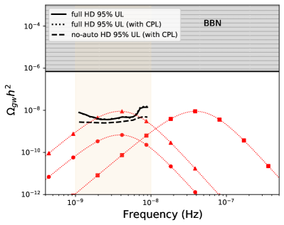
Figure 1: The 95% credibility Bayesian upper limits on the energy density of a free-spectrum SGWB based on the PPTA data. The solid, dotted and dashed black curves indicate results under different assumptions (hypotheses H2, H3 and H4 in Table 1, respectively, where the FOPT spectrum is substituted with the free spectrum). The region excluded by BBN cyburt2005new is shaded grey. Red curves with filled markers show examples of the spectrum predicted in the FOPT model, with $(\beta/H_{*})^{-1}=0.1$, and varying parameters $(\alpha,\,T_{*})=\{(0.2,\,3~{}\textrm{MeV})\ \textrm{(circle)},\,(0.5,3~{}\textrm{MeV})\ \textrm{(triangle)},(0.5,\,30~{}\textrm{MeV})\ \textrm{(square)}\}$, respectively.

Table 1: Description of hypotheses tested in this work and the Bayes factors between them.

Hypothesis	Pulsar noise	CPL process	HD process FOPT spectrum	Bayes Factors	Parameter Estimation (median and 1-$\sigma$ interval)
					$T_{*}$/MeV, $\alpha\times 10^{3}$, $\beta/H_{*}$	$A_{\rm CPL}$, $\gamma_{\rm CPL}$
H0:Pulsar Noise	✓
H1:CPL	✓	✓		$10^{2.9}$ (against H0)		$-14.45_{-0.64}^{+0.62}$,$3.31_{-1.53}^{+1.36}$
H2:FOPT	✓		✓(full HD)	$10^{1.8}$ (against H0)	$7.4_{-4.7}^{+11.9}$, $271_{-92}^{+165}$, $9.9^{+11.4}_{-5.4}$
H3:FOPT1	✓	✓	✓(full HD)	1.04 (against H1)	$9.6_{-9.2}^{+232.2}$, $3.8_{-3.4}^{+27.9}$, $854^{+9622}_{-782}$	$-14.51_{-0.68}^{+0.64}$,$3.36_{-1.54}^{+1.39}$
H4:FOPT2	✓	✓	✓(no-auto HD)	0.96 (against H1)	$10.9_{-10.6}^{+290.5}$, $3.2_{-2.8}^{+19.9}$, $1053^{+11256}_{-962}$	$-14.45_{-0.64}^{+0.62}$,$3.27_{-1.54}^{+1.37}$

We show in Fig. 1 the 95% credibility upper limits on the energy density of a SGWB in the $10^{-9}-10^{-8}$ Hz frequency range. The SGWB is characterised with a free spectrum. We note that the upper limits are almost unaffected by the inclusion of a CPL process. This is due to the choice of priors for the free-spectrum SGWB amplitude (uniform) and the CPL amplitude (log-uniform); see Table S1 in the Supplemental Material for details. We choose a uniform amplitude prior for the SGWB because it results in more conservative upper limits than the log-uniform prior. The upper limits are slightly more constraining for the case with only no-auto HD correlation included. Our results improve significantly upon the Big Bang nucleosynthesis (BBN cyburt2005new ) limit by two orders of magnitude in the frequency range considered in this work.

In the search for a FOPT signal, we consider three cases, listed as H2, H3 and H4 in Table 1, respectively. In H2, we assume that there is no CPL process. In both H3 and H4, a CPL process is included. In H3, we include the full HD correlation induced by a SGWB, whereas in H4 only the off-diagonal correlation (denoted as no-auto HD) is used. For comparison, we also consider H1 where we assume there is only a CPL process.

We summarize the hypotheses tested in this work and the Bayes factors between them in Table 1. First, being consistent with a separate analysis Boris21PPTAcrn , we find a strong evidence ($\rm{BF}\sim 10^{2.9}$) for a CPL process, if we follow the same analysis procedure/assumptions in Ref Arzoumanian:2020vkk . We then search for evidence of phase-transition gravitational waves. Without adding a CPL term (H2), we obtain a BF of $10^{1.8}$ in favour of the FOPT signal, which is less significant than that of CPL process (H1). Nevertheless, we show the posterior distributions of the FOPT model parameters in Fig. S1 of the Supplemental Material.

Since the origin of the apparent CPL process is still an open question, we take a conservative approach by assuming that there are unknown systematic errors that can be approximated by a CPL process. Under hypotheses H3 and H4, the evidence of the FOPT signal is negligible ($\rm{BF}\sim 1$).

In Fig. 2, we show the exclusion contours (at the 95% credible level) on FOPT model parameters for $\alpha=$ 0.2, 0.5, and 1. There are a few noteworthy features. First, the constraints become tighter for a larger value of $\alpha$ (i.e., larger phase transition strength). Second, the excluded range of phase-transition temperature $T_{*}$ is greater for longer phase-transition duration (i.e., larger $(\beta/H_{*})^{-1}$). Third, the excluded parameter space is larger for the case of no-auto HD correlation. This is because the FOPT models is slightly disfavoured by the data when auto-correlation of the SGWB is subtracted (see Table 1). Compared with the BBN bound on the phase transition temperature ($T_{*}>1$ MeV), our results are more sensitive when $1\ {\rm MeV}<T_{*}<100\ {\rm MeV}$.

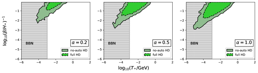
Figure 2: The PPTA exclusion contours (at 95% C.L.) on FOPT parameters $\log_{10}(T_{*}/{\rm GeV})$ and $\log_{10}[(\beta/H_{*})^{-1}]$, for $\alpha=0.2$, 0.5, and 1.0.

V Conclusion

Pulsar timing arrays provide a unique way to detect gravitational waves in the nanohertz frequency range ($10^{-9}$ Hz to $10^{-7}$ Hz), enabling the search for an SGWB potentially produced from cosmological phase transitions at low phase-transition temperatures ($\sim 1$ MeV). In the PPTA second Data Release kerr2020parkes , we search for the SGWB induced by first-order phase transitions of the early Universe. Assuming there is an unknown systematic error that can be approximated by a CPL process, we find no evidence for a Hellings-Downs spatial correlation induced by the phase-transition gravitational wave signal. We are able to exclude a significant parameter space of cosmological phase transitions that is not probed by previous observations. We find that phase transitions can be effectively constrained by the PPTA data for phase-transition temperatures of $\sim 1-100$ MeV and durations $(\beta/H_{*})^{-1}\sim 10^{-2}-10^{-1}$, which are within predictions from low-scale dark phase-transition models Ratzinger:2020koh ; Bian:2020urb ; Breitbach:2018ddu and cosmological first-order QCD phase transitions Caprini:2010xv . The results therefore place constraints on the new physics admitting a first-order phase transition at low-energy scales in the early Universe, and provide an alternative way to probe particle physics at low-energy scales.

Note added.—Recently the NANOGrav collaboration also performed a search for the gravitational-wave background from the FOPT in their 12.5-year data set NANOGrav21fopt . In that work, the gravitational-wave signal from phase transitions was proposed as a possible interpretation of the detected CPL process. As pointed out in Ref. Boris21PPTAcrn , the detection of a CPL process might suffer from model misspecification. Therefore, we consider the feature found in our data to be a noise component of unknown origin and derive constraints on the FOPT parameters. Better understanding of the nature of the CPL process requires longer data sets and more pulsars which might be available through the International Pulsar Timing Array IPTAdr2 in the future.

VI acknowledgements

We thank the referees for very useful comments. This work has been carried out by the Parkes Pulsar Timing Array, which is part of the International Pulsar Timing Array. The Parkes radio telescope (“Murriyang”) is part of the Australia Telescope, which is funded by the Commonwealth Government for operation as a National Facility managed by CSIRO. This work is supported in part by the National Key Research and Development Program of China under Grant No. 2020YFC2201501. XX is supported by Deutsche Forschungsgemeinschaft under Germany’s Excellence Strategy EXC2121 “Quantum Universe” - 390833306. LB is supported by the National Natural Science Foundation of China (NSFC) under the grants No. 12075041 and No. 12047564, the Fundamental Research Funds for the Central Universities of China (No. 2021CDJQY-011 and No. 2020CDJQY-Z003), and Chongqing Natural Science Foundation (Grant No. cstc2020jcyj-msxmX0814). JS is supported by the NSFC under Grants No. 12025507, No. 11690022, No. 11947302, by the Strategic Priority Research Program and Key Research Program of Frontier Science of the Chinese Academy of Sciences (CAS) under Grants No. XDB21010200, No. XDB23010000, No. XDPB15, No. ZDBS-LY-7003, and by the CAS Project for Young Scientists in Basic Research under Grant No. YSBR-006. QY is supported by CAS and the Program for Innovative Talents and Entrepreneur in Jiangsu. XZ was supported by ARC CE170100004. SD is the recipient of an Australian Research Council Discovery Early Career Award, project DE210101738 funded by the Australian Government. RMS is the recipient of Australian Research Council Future Fellowship FT190100155.

Supplemental Material

.1 Formalism of Pulsar Intrinsic Red Noise

The spin noise (for all pulsar ToAs) is parameterized as a power-law of frequency

$$S_{\rm spin}(f)=\frac{A_{s}^{2}}{12\pi^{2}}\left(\frac{f}{{\rm yr}^{-1}}\right)^{-\gamma_{s}}{\rm yr}^{3}.$$ (6)

The band noise is the same as spin noise, but only for ToAs of a certain photon frequency band,

$$S_{\rm band}(f)=\frac{A_{b}^{2}}{12\pi^{2}}\left(\frac{f}{{\rm yr}^{-1}}\right)^{-\gamma_{b}}{\rm yr}^{3}.$$ (7)

The dispersion measure (DM) noise applies to all pulsar ToAs, but correlates between different observing photon frequencies, as

$$S^{ij}_{\rm DM}(f)=\frac{A_{\rm DM}^{2}}{12\pi^{2}}\left(\frac{f}{{\rm yr}^{-1}}\right)^{-\gamma_{\rm DM}}{\rm yr}^{3}\left(\frac{\nu_{i}}{\nu_{\rm ref}}\right)^{-2}\left(\frac{\nu_{j}}{\nu_{\rm ref}}\right)^{-2},$$ (8)

where $\nu_{i}$ and $\nu_{j}$ are photon frequencies of the $i$th and $j$th ToA, $\nu_{\rm ref}=1400$ MHz is a reference frequency. The chromatic red noise is

$$S^{ij}_{\rm chrom}(f)=\frac{A_{c}^{2}}{12\pi^{2}}\left(\frac{f}{{\rm yr}^{-1}}\right)^{-\gamma_{c}}{\rm yr}^{3}\left(\frac{\nu_{i}}{\nu_{\rm ref}}\right)^{-n}\left(\frac{\nu_{j}}{\nu_{\rm ref}}\right)^{-n},$$ (9)

where $n$ variates from pulsar to pulsar.

The CPL process for all pulsars is

$$S_{\rm CPL}(f)=\frac{A_{\rm CPL}^{2}}{12\pi^{2}}\left(\frac{f}{{\rm yr}^{-1}}\right)^{-\gamma_{\rm CPL}}{\rm yr}^{3}.$$ (10)

The correlation $C_{ij}$ between ToA residuals is written as

$$C^{ij}_{\rm red}=\int_{f_{L}}{\tt d}f\left(\sum S^{ij}(f)\right)\cos\left(2\pi f(t_{i}-t_{j})\right).$$ (11)

where $\sum$ represents the summation over all red contributions, including noises, CPL process and gravitational wave background signals. For pulsar noises Eq. (6-9), $f_{L}=1/T$, $T$ is the duration of observation for the pulsar, The time-frequency method is adopted to approximate the integrals, and 30 linearly spaced frequency modes are chosen, i.e., $f_{i}=i/T$, $i=1...30$. For the CPL process Eq. (10) and all gravitational wave background signals, we use 20 logarithmically spaced frequency modes between $10^{-9}$ Hz and $10^{-8}$ Hz.

Table 2: Description and priors of the model parameters. The model of pulsar intrinsic noise we use is the same as ref. goncharov2020identifying , therefore no redundant description will be given here.

	Parameter	Prior	Description
CPL Process Parameters	$A_{\rm CPL}$	log-U[$10^{-18}$,$10^{-11}$]	one per PTA
	$\gamma_{\rm CPL}$	U[$0$,$7$]	one per PTA
FOPT Parameters	$\alpha$	log-U[$10^{-5}$,$1$]	one per PTA
	$(\beta/H_{*})^{-1}$	log-U[$10^{-6}$,$1$]	one per PTA
	$T_{*}$ (GeV)	log-U[$10^{-6}$,$10^{2}$]	one per PTA
Free Spectrum Parameters	$\sqrt{\Omega_{gw}(f_{i})h^{2}}$	U[$10^{-10}$,$10^{0}$]	20 per PTA
BayesEphem [12] Parameters	$z_{\rm drift}$	U[$-10^{-9}$,$10^{-9}$]	one per PTA
	$\Delta M_{\rm Jupiter}$	N$(0,1.5\times 10^{-11})$	one per PTA
	$\Delta M_{\rm Saturn}$	N$(0,8.2\times 10^{-12})$	one per PTA
	$\Delta M_{\rm Uranus}$	N$(0,5.7\times 10^{-11})$	one per PTA
	$\Delta M_{\rm Neptune}$	N$(0,7.9\times 10^{-11})$	one per PTA
	${\rm PCA}_{i}$	U[$-0.05$,$0.05$]	six per PTA

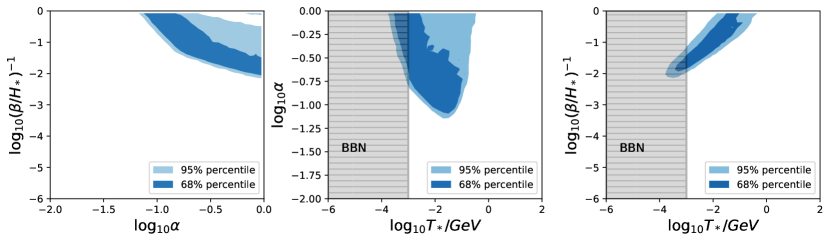
Figure 3: Posterior probability distributions of the FOPT parameters assuming no CPL process (under the H2 hypothesis in Table I). For each panel the other parameter is marginalized within its prior range. The excluded region from BBN cyburt2005new is shown as a grey shaded band.

.2 On the SMBBH Interpretation for the Common Power-Law Excess

The constraints on the FOPT model parameters in the SMBBH + FOPT hypothesis are found to be similar with those of H3 and H4, as can be seen in Fig. 4. The power spectral density of the SMBBH signal is written as

$$S_{\rm SMBBH}(f)=\frac{A_{\rm SMBBH}^{2}}{12\pi^{2}}\left(\frac{f}{{\rm yr}^{-1}}\right)^{-\gamma_{\rm SMBBH}}{\rm yr}^{3},$$ (12)

where the prior for $\log_{10}(A_{\rm SMBBH})$ is uniformly distributed from $-18$ and $-14$ and $\gamma_{\rm SMBBH}$ is fixed at $13/3$.

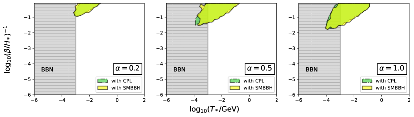
Figure 4: The PPTA exclusion contours (at 95% C.L.) on FOPT parameters $\log_{10}(T_{*}/{\rm GeV})$ and $\log_{10}[(\beta/H_{*})^{-1}]$ in the presence of a gravitational-wave background from supermassive binary black holes (SMBBH; in yellow) or a CPL process (green), for $\alpha=0.2$, 0.5, and 1.0. In both cases, we make use of the full-HD correlation in the analysis.

References

- (1) B. P. Abbott et al., “Observation of gravitational waves from a binary black hole merger,” Physical review letters, vol. 116, no. 6, p. 061102, 2016.
- (2) B. Abbott et al., “Gwtc-1: a gravitational-wave transient catalog of compact binary mergers observed by ligo and virgo during the first and second observing runs,” Physical Review X, vol. 9, no. 3, p. 031040, 2019.
- (3) R. Abbott et al., “GWTC-2: Compact Binary Coalescences Observed by LIGO and Virgo during the First Half of the Third Observing Run,” Physical Review X, vol. 11, p. 021053, Apr. 2021.
- (4) B. Abbott et al., “Prospects for Observing and Localizing Gravitational-Wave Transients with Advanced LIGO, Advanced Virgo and KAGRA,” Living Rev. Rel., vol. 21, no. 1, p. 3, 2018.
- (5) P. Amaro-Seoane et al., “Laser Interferometer Space Antenna,” arxiv:1702.00786, 2017.
- (6) C. Caprini et al., “Detecting gravitational waves from cosmological phase transitions with LISA: an update,” JCAP, vol. 03, p. 024, 2020.
- (7) R. N. Manchester et al., “The parkes pulsar timing array project,” Publications of the Astronomical Society of Australia, vol. 30, 2013.
- (8) G. Desvignes et al., “High-precision timing of 42 millisecond pulsars with the European Pulsar Timing Array,” Mon. Not. Roy. Astron. Soc. , vol. 458, pp. 3341–3380, May 2016.
- (9) M. F. Alam et al., “The NANOGrav 12.5 yr Data Set: Observations and Narrowband Timing of 47 Millisecond Pulsars,” Astrophys. J. Supp. , vol. 252, p. 4, Jan. 2021.
- (10) L. Lentati et al., “European Pulsar Timing Array Limits On An Isotropic Stochastic Gravitational-Wave Background,” Mon. Not. Roy. Astron. Soc., vol. 453, no. 3, pp. 2576–2598, 2015.
- (11) C. Caprini and D. G. Figueroa, “Cosmological Backgrounds of Gravitational Waves,” Class. Quant. Grav., vol. 35, no. 16, p. 163001, 2018.
- (12) Z. Arzoumanian et al., “The NANOGrav 11-year Data Set: Pulsar-timing Constraints On The Stochastic Gravitational-wave Background,” Astrophys. J., vol. 859, no. 1, p. 47, 2018.
- (13) J. Garcia-Bellido, M. Peloso, and C. Unal, “Gravitational Wave signatures of inflationary models from Primordial Black Hole Dark Matter,” JCAP, vol. 09, p. 013, 2017.
- (14) L. Barack et al., “Black holes, gravitational waves and fundamental physics: a roadmap,” Class. Quant. Grav., vol. 36, no. 14, p. 143001, 2019.
- (15) C. Caprini, R. Durrer, and X. Siemens, “Detection of gravitational waves from the QCD phase transition with pulsar timing arrays,” Phys. Rev. D, vol. 82, p. 063511, 2010.
- (16) M. Breitbach, J. Kopp, E. Madge, T. Opferkuch, and P. Schwaller, “Dark, Cold, and Noisy: Constraining Secluded Hidden Sectors with Gravitational Waves,” JCAP, vol. 07, p. 007, 2019.
- (17) M. D’Onofrio, K. Rummukainen, and A. Tranberg, “Sphaleron Rate in the Minimal Standard Model,” Phys. Rev. Lett., vol. 113, no. 14, p. 141602, 2014.
- (18) J. R. Espinosa, T. Konstandin, and F. Riva, “Strong Electroweak Phase Transitions in the Standard Model with a Singlet,” Nucl. Phys. B, vol. 854, pp. 592–630, 2012.
- (19) S. Profumo, M. J. Ramsey-Musolf, C. L. Wainwright, and P. Winslow, “Singlet-catalyzed electroweak phase transitions and precision Higgs boson studies,” Phys. Rev. D, vol. 91, no. 3, p. 035018, 2015.
- (20) M. Jiang, L. Bian, W. Huang, and J. Shu, “Impact of a complex singlet: Electroweak baryogenesis and dark matter,” Phys. Rev. D, vol. 93, no. 6, p. 065032, 2016.
- (21) S. Profumo, M. J. Ramsey-Musolf, and G. Shaughnessy, “Singlet Higgs phenomenology and the electroweak phase transition,” JHEP, vol. 08, p. 010, 2007.
- (22) J. O. Andersen, T. Gorda, A. Helset, L. Niemi, T. V. I. Tenkanen, A. Tranberg, A. Vuorinen, and D. J. Weir, “Nonperturbative Analysis of the Electroweak Phase Transition in the Two Higgs Doublet Model,” Phys. Rev. Lett., vol. 121, no. 19, p. 191802, 2018.
- (23) J. Bernon, L. Bian, and Y. Jiang, “A new insight into the phase transition in the early Universe with two Higgs doublets,” JHEP, vol. 05, p. 151, 2018.
- (24) G. Dorsch, S. Huber, and J. No, “A strong electroweak phase transition in the 2HDM after LHC8,” JHEP, vol. 10, p. 029, 2013.
- (25) P. Basler, M. Krause, M. Muhlleitner, J. Wittbrodt, and A. Wlotzka, “Strong First Order Electroweak Phase Transition in the CP-Conserving 2HDM Revisited,” JHEP, vol. 02, p. 121, 2017.
- (26) J. Kozaczuk, S. Profumo, L. S. Haskins, and C. L. Wainwright, “Cosmological Phase Transitions and their Properties in the NMSSM,” JHEP, vol. 01, p. 144, 2015.
- (27) S. J. Huber, T. Konstandin, G. Nardini, and I. Rues, “Detectable Gravitational Waves from Very Strong Phase Transitions in the General NMSSM,” JCAP, vol. 03, p. 036, 2016.
- (28) L. Bian, H.-K. Guo, and J. Shu, “Gravitational Waves, baryon asymmetry of the universe and electric dipole moment in the CP-violating NMSSM,” Chin. Phys. C, vol. 42, no. 9, p. 093106, 2018. [Erratum: Chin.Phys.C 43, 129101 (2019)].
- (29) J. R. Espinosa, B. Gripaios, T. Konstandin, and F. Riva, “Electroweak Baryogenesis in Non-minimal Composite Higgs Models,” JCAP, vol. 01, p. 012, 2012.
- (30) L. Bian, Y. Wu, and K.-P. Xie, “Electroweak phase transition with composite Higgs models: calculability, gravitational waves and collider searches,” JHEP, vol. 12, p. 028, 2019.
- (31) P. Schwaller, “Gravitational Waves from a Dark Phase Transition,” Phys. Rev. Lett., vol. 115, no. 18, p. 181101, 2015.
- (32) L. Bian, R.-G. Cai, J. Liu, X.-Y. Yang, and R. Zhou, “Evidence for different gravitational-wave sources in the NANOGrav dataset,” Phys. Rev. D, vol. 103, no. 8, p. L081301, 2021.
- (33) R. S. Foster and D. Backer, “Constructing a pulsar timing array,” The Astrophysical Journal, vol. 361, pp. 300–308, 1990.
- (34) R. Hellings and G. Downs, “Upper limits on the isotropic gravitational radiation background from pulsar timing analysis,” The Astrophysical Journal, vol. 265, pp. L39–L42, 1983.
- (35) C. Caprini, R. Durrer, and G. Servant, “Gravitational wave generation from bubble collisions in first-order phase transitions: An analytic approach,” Phys. Rev. D, vol. 77, p. 124015, 2008.
- (36) S. J. Huber and T. Konstandin, “Gravitational Wave Production by Collisions: More Bubbles,” JCAP, vol. 09, p. 022, 2008.
- (37) M. Hindmarsh, S. J. Huber, K. Rummukainen, and D. J. Weir, “Shape of the acoustic gravitational wave power spectrum from a first order phase transition,” Phys. Rev. D, vol. 96, no. 10, p. 103520, 2017. [Erratum: Phys.Rev.D 101, 089902 (2020)].
- (38) M. Hindmarsh, S. J. Huber, K. Rummukainen, and D. J. Weir, “Gravitational waves from the sound of a first order phase transition,” Phys. Rev. Lett., vol. 112, p. 041301, 2014.
- (39) M. Hindmarsh, “Sound shell model for acoustic gravitational wave production at a first-order phase transition in the early Universe,” Phys. Rev. Lett., vol. 120, no. 7, p. 071301, 2018.
- (40) D. Cutting, M. Hindmarsh, and D. J. Weir, “Vorticity, kinetic energy, and suppressed gravitational wave production in strong first order phase transitions,” Phys. Rev. Lett., vol. 125, no. 2, p. 021302, 2020.
- (41) M. Hindmarsh, S. J. Huber, K. Rummukainen, and D. J. Weir, “Numerical simulations of acoustically generated gravitational waves at a first order phase transition,” Physical Review D, vol. 92, no. 12, p. 123009, 2015.
- (42) C. Caprini, R. Durrer, and G. Servant, “The stochastic gravitational wave background from turbulence and magnetic fields generated by a first-order phase transition,” JCAP, vol. 12, p. 024, 2009.
- (43) C. Caprini et al., “Science with the space-based interferometer eLISA. II: Gravitational waves from cosmological phase transitions,” JCAP, vol. 04, p. 001, 2016.
- (44) J. Ellis, M. Lewicki, and J. M. No, “On the Maximal Strength of a First-Order Electroweak Phase Transition and its Gravitational Wave Signal,” JCAP, vol. 04, p. 003, 2019.
- (45) J. Ellis, M. Lewicki, J. M. No, and V. Vaskonen, “Gravitational wave energy budget in strongly supercooled phase transitions,” JCAP, vol. 06, p. 024, 2019.
- (46) J. R. Espinosa, T. Konstandin, J. M. No, and G. Servant, “Energy Budget of Cosmological First-order Phase Transitions,” JCAP, vol. 06, p. 028, 2010.
- (47) L. Husdal, “On effective degrees of freedom in the early universe,” Galaxies, vol. 4, no. 4, p. 78, 2016.
- (48) B. Allen and J. D. Romano, “Detecting a stochastic background of gravitational radiation: Signal processing strategies and sensitivities,” Physical Review D, vol. 59, no. 10, p. 102001, 1999.
- (49) M. Maggiore, “Gravitational wave experiments and early universe cosmology,” Physics Reports, vol. 331, no. 6, pp. 283–367, 2000.
- (50) B. Goncharov et al., “Identifying and mitigating noise sources in precision pulsar timing data sets,” Mon. Not. Roy. Astron. Soc. , vol. 502, pp. 478–493, Mar. 2021.
- (51) G. Hobbs, R. Edwards, and R. Manchester, “Tempo2, a new pulsar-timing package–i. an overview,” Monthly Notices of the Royal Astronomical Society, vol. 369, no. 2, pp. 655–672, 2006.
- (52) R. T. Edwards, G. Hobbs, and R. Manchester, “Tempo2, a new pulsar timing package–ii. the timing model and precision estimates,” Monthly Notices of the Royal Astronomical Society, vol. 372, no. 4, pp. 1549–1574, 2006.
- (53) R. van Haasteren, Y. Levin, G. Janssen, K. Lazaridis, M. Kramer, B. Stappers, G. Desvignes, M. Purver, A. Lyne, R. Ferdman, et al., “Placing limits on the stochastic gravitational-wave background using european pulsar timing array data,” Monthly Notices of the Royal Astronomical Society, vol. 414, no. 4, pp. 3117–3128, 2011.
- (54) K. Liu, J. Verbiest, M. Kramer, B. Stappers, W. van Straten, and J. Cordes, “Prospects for high-precision pulsar timing,” Monthly Notices of the Royal Astronomical Society, vol. 417, no. 4, pp. 2916–2926, 2011.
- (55) K. Liu, E. Keane, K. Lee, M. Kramer, J. Cordes, and M. Purver, “Profile-shape stability and phase-jitter analyses of millisecond pulsars,” Monthly Notices of the Royal Astronomical Society, vol. 420, no. 1, pp. 361–368, 2012.
- (56) Z. Arzoumanian, A. Brazier, S. Burke-Spolaor, S. Chamberlin, S. Chatterjee, B. Christy, J. M. Cordes, N. Cornish, K. Crowter, P. B. Demorest, et al., “The nanograv nine-year data set: observations, arrival time measurements, and analysis of 37 millisecond pulsars,” The Astrophysical Journal, vol. 813, no. 1, p. 65, 2015.
- (57) R. van Haasteren and Y. Levin, “Understanding and analysing time-correlated stochastic signals in pulsar timing,” Monthly Notices of the Royal Astronomical Society, vol. 428, no. 2, pp. 1147–1159, 2013.
- (58) R. van Haasteren and M. Vallisneri, “Low-rank approximations for large stationary covariance matrices, as used in the Bayesian and generalized-least-squares analysis of pulsar-timing data,” Mon. Not. Roy. Astron. Soc. , vol. 446, pp. 1170–1174, Jan. 2015.
- (59) R. Caballero, K. Lee, L. Lentati, G. Desvignes, D. Champion, J. Verbiest, G. Janssen, B. Stappers, M. Kramer, P. Lazarus, et al., “The noise properties of 42 millisecond pulsars from the european pulsar timing array and their impact on gravitational-wave searches,” Monthly Notices of the Royal Astronomical Society, vol. 457, no. 4, pp. 4421–4440, 2016.
- (60) L. Lentati, R. M. Shannon, W. A. Coles, J. P. Verbiest, R. van Haasteren, J. Ellis, R. Caballero, R. N. Manchester, Z. Arzoumanian, S. Babak, et al., “From spin noise to systematics: stochastic processes in the first international pulsar timing array data release,” Monthly Notices of the Royal Astronomical Society, vol. 458, no. 2, pp. 2161–2187, 2016.
- (61) X. You, G. Hobbs, W. A. Coles, R. N. Manchester, R. Edwards, M. Bailes, J. Sarkissian, J. P. Verbiest, W. Van Straten, A. Hotan, et al., “Dispersion measure variations and their effect on precision pulsar timing,” Monthly Notices of the Royal Astronomical Society, vol. 378, no. 2, pp. 493–506, 2007.
- (62) M. Keith, W. Coles, R. Shannon, G. Hobbs, R. Manchester, M. Bailes, N. Bhat, S. Burke-Spolaor, D. Champion, A. Chaudhary, et al., “Measurement and correction of variations in interstellar dispersion in high-precision pulsar timing,” Monthly Notices of the Royal Astronomical Society, vol. 429, no. 3, pp. 2161–2174, 2013.
- (63) Z. Arzoumanian et al., “The NANOGrav 12.5 yr Data Set: Search for an Isotropic Stochastic Gravitational-wave Background,” Astrophys. J. Lett. , vol. 905, p. L34, Dec. 2020.
- (64) B. Goncharov et al., “On the evidence for a common-spectrum process in the search for the nanohertz gravitational-wave background with the Parkes Pulsar Timing Array,” arXiv e-prints, p. arXiv:2107.12112, July 2021.
- (65) J. M. Dickey, “The weighted likelihood ratio, linear hypotheses on normal location parameters,” The Annals of Mathematical Statistics, pp. 204–223, 1971.
- (66) R. H. Cyburt, B. D. Fields, K. A. Olive, and E. Skillman, “New bbn limits on physics beyond the standard model from 4he,” Astroparticle Physics, vol. 23, no. 3, pp. 313–323, 2005.
- (67) M. Kerr et al., “The Parkes Pulsar Timing Array project: second data release,” Publications of the Astronomical Society of Australia, vol. 37, p. e020, June 2020.
- (68) W. Ratzinger and P. Schwaller, “Whispers from the dark side: Confronting light new physics with NANOGrav data,” SciPost Phys., vol. 10, p. 047, 2021.
- (69) Z. Arzoumanian et al., “Searching For Gravitational Waves From Cosmological Phase Transitions With The NANOGrav 12.5-year dataset,” arXiv e-prints, p. arXiv:2104.13930, Apr. 2021.
- (70) B. B. P. Perera et al., “The International Pulsar Timing Array: second data release,” Mon. Not. Roy. Astron. Soc. , vol. 490, pp. 4666–4687, Dec. 2019.