Player Tracking and Identification in Ice Hockey
Abstract
Tracking and identifying players is a fundamental step in computer vision-based ice hockey analytics. The data generated by tracking is used in many other downstream tasks, such as game event detection and game strategy analysis. Player tracking and identification is a challenging problem since the motion of players in hockey is fast-paced and non-linear when compared to pedestrians. There is also significant camera panning and zooming in hockey broadcast video. Identifying players in ice hockey is challenging since the players of the same team appear almost identical, with the jersey number the only consistent discriminating factor between players. To address this problem, an automated system to track and identify players in broadcast NHL hockey videos is introduced. The system is composed of three components (1) player tracking, (2) team identification and (3) player identification. Due to the absence of publicly available datasets, the datasets used to train the three components are annotated manually. Player tracking is performed with the help of a state of the art tracking algorithm obtaining a Multi-Object Tracking Accuracy (MOTA) score of . For team identification, away-team jerseys are grouped into a single class and home-team jerseys are grouped in classes according to their jersey color. A convolutional neural network is then trained on the team identification dataset. The team identification network obtains an accuracy of on the test set. A novel player identification model is introduced that utilizes a temporal one-dimensional convolutional network to identify players from player bounding box sequences. The player identification model further takes advantage of the available NHL game roster data to obtain a player identification accuracy of .
Index Terms:
computer vision, broadcast video, National Hockey League, jersey numberI Introduction
Ice hockey is a popular sport played by millions of people [21]. Being a team sport, knowing the location of players on the ice rink is essential for analyzing the game strategy and player performance. The locations of the players on the rink during the game are used by coaches, scouts, and statisticians for analyzing the play. Although player location data can be obtained manually, the process of labelling data by hand on a per-game basis is extremely tedious and time consuming. Therefore, an automated computer vision-based player tracking and identification system is of high utility.
In this paper, we introduce an automated system to track and identify players in broadcast National Hockey League (NHL) videos. Referees, being a part of the game, are also tracked and identified separately from players. The input to the system is broadcast NHL clips from the main camera view (i.e., camera located in the stands above the centre ice line) and the output are player trajectories along with their identities. Since there are no publicly available datasets for ice hockey player tracking, team identification, and player identification, we annotate our own datasets for each of these problems. The previous papers in ice hockey player tracking [9, 35] make use of hand crafted features for detection and re-identification. Therefore, we perform experiments with five state of the art tracking algorithms [8, 4, 50, 6, 52] on our hockey player tracking dataset and evaluate their performance. The output of the player tracking algorithm is a temporal sequence of player bounding boxes, called player tracklets.
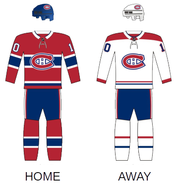
Posing team identification as a classification problem with each team treated as a separate class would be impractical since (1) this will result in a large number of classes, and (2) the same NHL team wears two different colors based on whether it is the home or away team (Fig. 2). Therefore, instead of treating each team as a separate class, we treat the away (light) jerseys of all teams as a single class and cluster home jerseys based on their jersey color. Since referees are easily distinguishable from players, they are treated as a separate class.Based on this simple training data formation, hockey players can be classified into home and away teams. The team identification network obtains an accuracy of on the test set and does not require additional fine tuning on new games.

Unlike soccer and basketball [41] where player facial features and skin color are visible, a big challenge in player identification in hockey is that the players of the same team appear nearly identical due to having the same uniform as well as having similar physical size.. Therefore, we use jersey number for identifying players since it is the most prominent feature present on all player jerseys. Instead of classifying jersey numbers from static images [14, 26, 29], we identify a player’s jersey number from player tracklets. Player tracklets allow a model to process temporal context to identify a jersey number since that is likely to be visible in multiple frames of the tracklet. We introduce a temporal 1-dimensional convolutional neural network (1D CNN)-based network for identifying players from their tracklets. The network generates a higher accuracy than the previous work by Chan et al. [10] by without requiring any additional probability score aggregation model for inference.
The tracking, team identification, and player identification models are combined to form a holistic offline system to track and identify players and referees in the broadcast videos. Player tracking helps team identification by removing team identification errors in player tracklets through a simple majority voting. Additionally, based on the team identification output, we use the game roster data to further improve the identification performance of the automated system by an additional . The overall system is depicted in Fig. 1. The system is able to identify players from video with an accuracy of with a Multi-Object Tracking Accuracy (MOTA) score of and an Identification (IDF1) score of .
Five computer vision contributions are recognized applied to the game of ice hockey:
-
1.
New ice hockey datasets are introduced for player tracking, team identification, and player identification from tracklets.
-
2.
We compare and contrast several state-of-the-art tracking algorithms and analyze their performance and failure modes.
-
3.
A simple but efficient team identification algorithm for ice hockey is implemented.
-
4.
A temporal 1D CNN based player identification model is implemented that outperforms the current state of the art [10] by .
-
5.
A holistic system that combines tracking, team identification, and player identification models, along with making use of the team roster data, to track and identify players in broadcast ice hockey videos is established.
II Background
II-A Tracking
The objective of multi-object tracking (MOT) is to detect objects of interest in video frames and associate the detections with appropriate trajectories. Player tracking is an important problem in computer vision-based sports analytics, since player tracking combined with an automatic homography estimation system [24] is used to obtain absolute player locations on the sports rink. Also, various computer vision-based tasks, such as sports event detection [47, 39, 46], can be improved with player tracking data.
Tracking by detection (TBD) is a widely used approach for multi-object tracking. Tracking by detection consists of two steps: (1) detecting objects of interest (hockey players in our case) frame-by-frame in the video, then (2) linking player detections to produce tracks using a tracking algorithm. Detection is usually done with the help of a deep detector, such as Faster R-CNN [37] or YOLO [36]. For associating detections with trajectories, techniques such as Kalman filtering with Hungarian algorithm [6, 50, 52] and graphical inference [8, 42] are used. In recent literature, re-identification in tracking is commonly carried out with the help of deep CNNs using appearance [50, 8, 52] and pose features [42].
For sports player tracking, Sanguesa et al. [40] demonstrated that deep features perform better than classical hand crafted features for basketball player tracking. Lu et al. [31] perform player tracking in basketball using a Kalman filter. Theagarajan et al. [43] track players in soccer videos using the DeepSORT algorithm [50]. Hurault et al [20] introduce a self-supervised detection algorithm to detect small soccer players and track players in non-broadcast settings using a triplet loss trained re-identification mechanism, with embeddings obtained from the detector itself.
In ice hockey, Okuma et al. [35] track hockey players by introducing a particle filter combined with mixture particle filter (MPF) framework [48], along with an Adaboost [49] player detector. The MPF framework [48] allows the particle filter framework to handle multi-modality by modelling the posterior state distributions of objects as an component mixture. A disadvantage of the MPF framework is that the particles merge and split in the process and leads to loss of identities. Moreover, the algorithm did not have any mechanism to prevent identity switches and lost identities of players after occlusions. Cai et al. [9] improved upon [35] by using a bipartite matching for associating observations with targets instead of using the mixture particle framework. However, the algorithm is not trained or tested on broadcast videos, but performs tracking in the rink coordinate system after a manual homography calculation.
In ice hockey, prior published research [35, 9] perform player tracking with the help of handcrafted features for player detection and re-identification. In this paper we track and identify hockey players in broadcast NHL videos and analyze performance of several state-of-the-art deep tracking models on the ice hockey dataset.
II-B Player Identification
Identifying players and referees is one of the most important problems in computer vision-based sports analytics. Analyzing individual player actions and player performance from broadcast video is not feasible without detecting and identifying the player. Before the advent of deep learning methods, player identification was performed with the help of handcrafted features [53]. Although techniques for identifying players from body appearance exist [41], jersey number is the primary and most widely used feature for player identification, since it is observable and consistent throughout a game. Most deep learning based player identification approaches in the literature focus on identifying the player jersey number from single frames using a CNN [14, 26, 29]. Gerke et al. [14] were one of the first to use CNNs for soccer jersey number identification and found that deep learning approach outperforms handcrafted features. Li et al. [26] employed a semi-supervised spatial transformer network to help the CNN localize the jersey number in the player image. Liu et al. [29] use a pose-guided R-CNN for jersey digit localization and classification by introducing a human keypoint prediction branch to the network and a pose-guided regressor to generate digit proposals. Gerke et al. [15] also combined their single-frame based jersey classifier with soccer field constellation features to identify players. Vats et al. [45] use a multi-task learning loss based approach to identify jersey numbers from static images.
Zhang et al. [51] track and identify players in a multi-camera setting using a distinguishable deep representation of player identity using a coarse-to-fine framework. Lu et al. [31] use a variant of Expectation-Maximization (EM) algorithm to learn a Conditional Random Field (CRF) model composed of player identity and feature nodes. Chan et al. [10] use a combination of a CNN and long short term memory network (LSTM) [19] similar to the long term recurrent convolutional network (LRCN) by Dohnaue et al. [12] for identifying players from player sequences. The final inference in Chan el al. [10] is performed using a another CNN network applied over probability scores obtained from CNN LSTM network.
In this paper, we identify players using player tracklets with the help of a temporal 1D CNN. Our proposed inference scheme does not require the use of an additional network.
II-C Team Identification
Beyond knowing the identity of a player, the player must also be assigned to a team. Many sports analytics, such as “shot attempts” and “team formations”, require knowing the team to which each individual belongs. In sports leagues, teams differentiate themselves based on the colour and design of the jerseys worn by the players. In ice hockey, formulating team identification as a classification problem with each team treated as a separate class is not feasible since teams use different colored jerseys depending if they are the ’home’ or ’away’ team. Teams wear light- and dark-coloured jerseys depending on whether they are playing at their home venue or away venue (Fig. 2). Furthermore, each game in which new teams play would require fine-tuning [25].
Early work used colour histograms or colour features with a clustering approach to differentiate teams [3, 23, 13, 32, 30, 7, 44, 16, 34, 1]. This approach, while being lightweight, does not address occlusions, changes in illumination, and teams wearing similar jersey colours [3, 25]. Deep learning approaches have increased performance and generalizablitity of player classification models [22].
Istasse et al. [22] simultaneously segment and classify players in indoor basketball games. Players are segmented and classified in a system where no prior is known about the visual appearance of each team with associative embedding. A trained CNN outputs a player segmentation mask and, for each pixel, a feature vector that is similar for players belonging to the same team. Theagarajan and Bhanu [43] classify soccer players by team as part of a pipeline for generating tactical performance statistics by using triplet CNNs.
In ice hockey, Guo et al. [17] perform team identification using the color features of hockey player uniforms. For this purpose, the uniform region (central region) of the player’s bounding box is cropped. From this region, hue, saturation, and lightness (HSL) pixel values are extracted, and histograms of pixels in five essential color channels (i.e., green, yellow, blue, red, and white) are constructed. Finally, the player’s team identification is determined by the channel that contains the maximum proportions of pixels. Koshkina et al. [25] use contrastive learning to classify player bounding boxes in hockey games. This self-supervised learning approach uses a CNN trained with triplet loss to learn a feature space that best separates players into two teams. Over a sequence of initial frames, they first learn two k-means cluster centres, then associate players to teams.
III Technical Approach
III-A Player Tracking
III-A1 Dataset
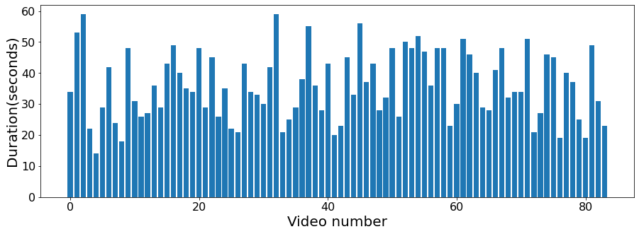
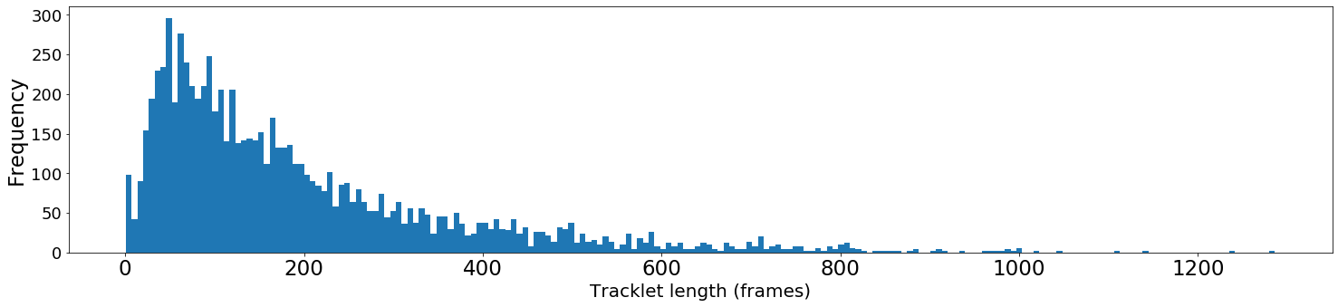
The player tracking dataset consists of a total of 84 broadcast NHL game clips with a frame rate of 30 frames per second (fps) and resolution of pixels. The average clip duration is seconds. The 84 video clips in the dataset are extracted from 25 NHL games. The duration of the clips in shown in Fig. 4. Each frame in a clip is annotated with player and referee bounding boxes and player identity consisting of player name and jersey number. The annotation is carried out with the help of open source CVAT tool111Found online at: https://github.com/openvinotoolkit/cvat. The dataset is split such that 58 clips are used for training, 13 clips for validation, and 13 clips for testing. To prevent any game-level bias affecting the results, the split is made at the game level, such that the training clips are obtained from 17 games, validation clips from 4 games and test split from 4 games, respectively.
III-A2 Methodology
We experimented with five state-of-the-art tracking algorithms on the hockey player tracking dataset. The algorithms include four online tracking algorithms [6, 50, 52, 4] and one offline tracking algorithm [8]. The best tracking performance (see Section IV) is achieved using the MOT Neural Solver tracking model [8] re-trained on the hockey dataset. MOT Neural Solver uses the popular tracking-by-detection paradigm.
In tracking by detection, the input is a set of object detections , where denotes the total number of detections in all video frames. A detection is represented by , where denotes the coordinates, width, and height of the detection bounding box. and represent the image pixels and timestamp corresponding to the detection. The goal is to find a set of trajectories that best explains where each is a time-ordered set of observations. The MOT Neural Solver models the tracking problem as an undirected graph , where is the set of nodes for player detections for all video frames. In the edge set , every pair of detections is connected so that trajectories with missed detections can be recovered. The problem of tracking is now posed as splitting the graph into disconnected components where each component is a trajectory . After computing each node (detection) embedding and edge embedding using a CNN, the model then solves a graph message passing problem. The message passing algorithm classifies whether an edge between two nodes in the graph belongs to the same player trajectory.
III-B Team Identification
III-B1 Dataset
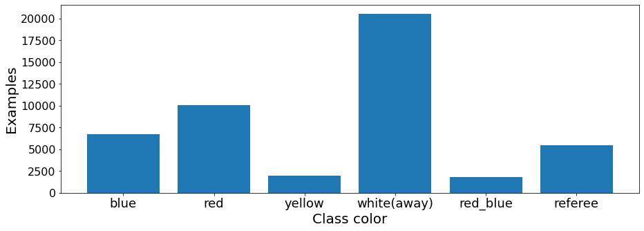
The team identification dataset is obtained from the same games and clips used in the player tracking dataset. The train/validation/test splits are also identical to player tracking data. We take advantage of the fact that the away team in NHL games usually wear a predominantly white colored jersey with color stripes and patches, and the home team wears a dark colored jersey. For example, the Toronto Maple Leafs and the Tampa Bay Lightning both have dark blue home jerseys and therefore can be put into a single ‘Blue’ class. We therefore build a dataset with five classes (blue, red, yellow, white, red-blue and referees) with each class composed of images with same dominant color. The data-class distribution is shown in Fig. 6. Fig. 5 shows an example of the blue class from the dataset. The training set consists of images. The validation and testing set contain and images respectively.
III-B2 Methodology
For team identification, we use a ResNet18 [18] pretrained on the ImageNet dataset [11], and train the network on the team identification dataset by replacing the final fully connected layer to output six classes. The images are scaled to a resolution of pixels for training. During inference, the network classifies whether a bounding box belongs to the away team (white color), the home team (dark color), or the referee class. For inferring the team for a player tracklet, the team identification model is applied to each image of the tracklet and a simple majority vote is used to assign a team to the tracklet. This way, the tracking algorithm helps team identification by resolving errors in team identification.
III-B3 Training Details
We use the Adam optimizer with an initial learning rate of .001 and a weight decay of .001 for optimization. The learning rate is reduced by a factor of at regular intervals during the training process. We do not perform data augmentation since performing color augmentation on white away jerseys makes it resemble colored home jerseys.
| Input: Player tracklet |
| ResNet18 backbone |
| Layer 1: Conv1D |
| (k = , s = , p = , d = ) |
| Batch Norm 1D |
| ReLU |
| Layer 2: Conv1D |
| (k = , s = , p = , d = ) |
| Batch Norm 1D |
| ReLU |
| Layer 3: Conv2D |
| (k = , s = , p = , d = ) |
| Batch Norm 1D |
| ReLU |
| Layer 4: Fully connected |
| Output |
III-C Player Identification
III-C1 Image Dataset
The player identification image dataset [45] consists of player bounding boxes obtained from 25 NHL games. The NHL game video frames are of resolution pixels. The dataset contains jersey number classes, including an additional class for no jersey number visible. The player head and bottom of the images are cropped such that only the jersey number (player torso) is visible. Images from games are used for training, four games for validation and four games for testing. The dataset is highly imbalanced such that the ratio between the most frequent and least frequent class is . The dataset covers a range of real-game scenarios such as occlusions, motion blur and self-occlusions.
III-C2 Tracklet Dataset
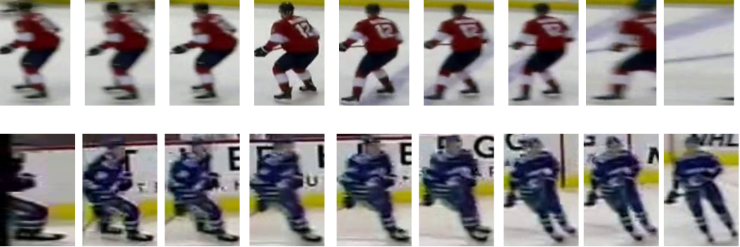
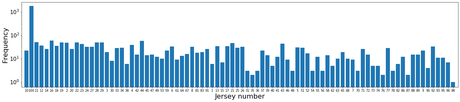
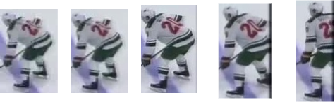
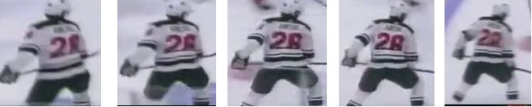
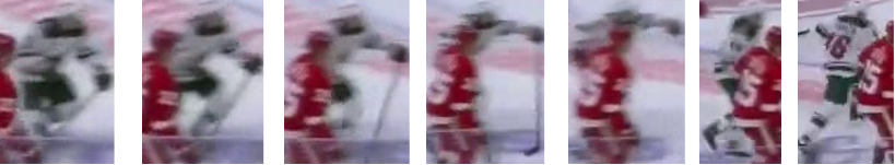
The player identification tracklet dataset consists of player tracklets. The tracklet bounding boxes and identities are annotated manually. The manually annotated tracklets simulate the output of a tracking algorithm. The tracklet length distribution is shown in Fig. 8. The average length of a player tracklet is frames (6.37 seconds in a 30 frame per second video). It is important to note that the player jersey number is visible in only a subset of tracklet frames. Fig. 7 illustrates two tracklet examples from the dataset. The dataset is divided into 86 jersey number classes with one class representing no jersey number visible. The class distribution is shown in Fig. 9. The dataset is heavily imbalanced with the class consisting of of tracklet examples. The training set contains tracklets, validation tracklets and test tracklets. The game-wise training/testing data split is identical in all the four datasets discussed.
III-C3 Network Architecture
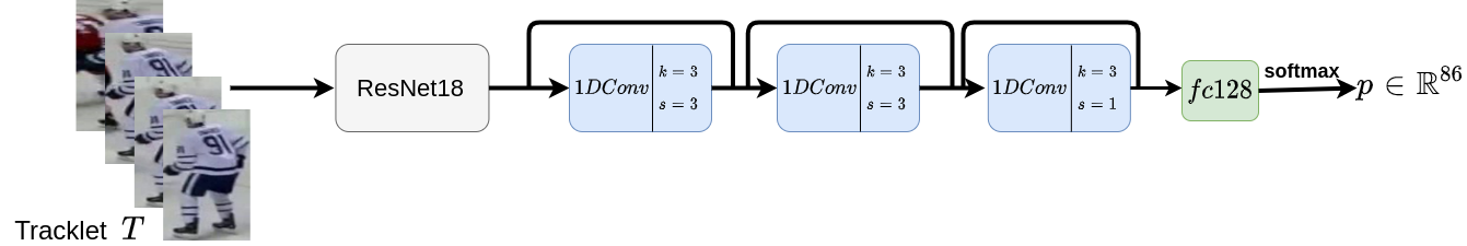
Let denote a player tracklet where each represents a player bounding box. The player head and bottom in the bounding box are cropped such that only the jersey number is visible. Each resized image corresponding to the bounding box is input into a backbone 2D CNN, which outputs a set of time-ordered features . The features are input into a 1D temporal convolutional network that outputs probability of the tracklet belonging to a particular jersey number class. The architecture of the 1D CNN is shown in Fig. 3.
The network consists of a ResNet18 [18] based 2D CNN backbone pretrained on the player identification image dataset (Section III-C1). The weights of the ResNet18 backbone network are kept frozen while training. The 2D CNN backbone is followed by three 1D convolutional blocks each consisting of a 1D convolutional layer, batch normalization, and ReLU activation. Each block has a kernel size of three and dilation of one. The first two blocks have a larger stride of three, so that the initial layers have a larger receptive field to take advantage of a large temporal context. Residual skip connections are added to aid learning. The exact architecture is shown in Table I. Finally, the activations obtained are pooled using mean pooling and passed through a fully connected layer with 128 units. The logits obtained are softmaxed to obtain jersey number probabilities. Note that the model accepts fixed length training sequences of length frames as input, but the training tracklets are hundreds of frames in length (Fig. 8). Therefore, tracklet frames are sampled with a random starting frame from the training tracklet. This serves as a form of data augmentation since at every training iteration, the network processes a randomly sampled set of frames from an input tracklet.
III-C4 Training Details
To address the severe class imbalance present in the tracklet dataset, the tracklets are sampled intelligently such that the class is sampled with a probability . The network is trained with the help of cross entropy loss. We use Adam optimizer for training with a initial learning rate of with a batch size of . The learning rate is reduced by a factor of after iteration numbers 2500, 5000, and 7500. Several data augmentation techniques such as random cropping, color jittering, and random rotation are also used. All experiments are performed on two Nvidia P-100 GPUs.
III-C5 Inference
During inference, we need to assign a single jersey number label to a test tracklet of bounding boxes . Here can be much greater than . So, a sliding window technique is used where the network is applied to the whole test tracklet with a stride of one frame to obtain window probabilities with each . The probabilities are aggregated to assign a single jersey number class to a tracklet. To aggregate the probabilities , we filter out the tracklets where the jersey number is visible. To do this we first train a ResNet18 classifier (same as the backbone of discussed in Section III-C3) on the player identification image dataset. The classifier is run on every image of the tracklet. A jersey number is assumed to be absent on a tracklet if the probability of the absence of jersey number is greater than a threshold for each image in the tracklet. The threshold is determined using the player identification validation set. The tracklets for which the jersey number is visible, the probabilities are averaged to obtain a single probability vector , which represents the probability distribution of the jersey number in the test tracklet . For post-processing, only those probability vectors are averaged for which .
The rationale behind using visibility filtering and post-processing step is that a large tracklet with hundreds of frames may have the number visible in only a few frames and therefore, a simple averaging of probabilities will often output . The proposed inference technique allows the network to ignore the window probabilities corresponding to the class if a number is visible in the tracklet. The whole algorithm is illustrated in Algorithm 1.
| Video number | IDF1 | MOTA | ID-switches | False positives (FP) | False negatives (FN) |
|---|---|---|---|---|---|
| 1 | |||||
| 2 | |||||
| 3 | |||||
| 4 | |||||
| 5 | |||||
| 6 | |||||
| 7 | |||||
| 8 | |||||
| 9 | |||||
| 10 | |||||
| 11 | |||||
| 12 | |||||
| 13 |
| Method | IDF1 | MOTA | ID-switches | False positives (FP) | False negatives (FN) |
| SORT [6] | |||||
| Deep SORT [50] | |||||
| Tracktor [4] | |||||
| FairMOT [52] | |||||
| MOT Neural Solver [8] | 62.9 | 94.5 | 431 |
III-D Overall System
The player tracking, team identification, and player identification methods discussed are combined together for tracking and identifying players and referees in broadcast video shots. Given a test video shot, we first run player detection and tracking to obtain a set of player tracklets . For each tracklet obtained, we run the player identification model to obtain the player identity. We take advantage of the fact that the player roster is available for NHL games through play-by-play data, hence we can focus only on players actually present in the team. To do this, we construct vectors and that contain information about which jersey numbers are present in the away and home teams, respectively. We refer to the vectors and as the roster vectors. Assuming we know the home and away roster, let be the set of jersey numbers present in the home team and be the set of jersey numbers present in away team. Let denote the probability of the jersey number present in the tracklet. Let denote the no-jersey number class and denote the index associated with jersey number in vector.
| (1) | ||||
| (2) |
similarly,
| (3) | ||||
| (4) |
We multiply the probability scores obtained from the player identification by if the player belongs to home team or if the player belongs to the away team. The determination of player team is done through the trained team identification model. The player identity is determined through
| (5) |
(where denotes element-wise multiplication) if the player belongs to home team, and
| (6) |
if the player belongs to the away team. The overall algorithm is summarized in Algorithm 2. Fig. 1 depicts the overall system.
IV Results
IV-A Player Tracking
The MOT Neural Solver algorithm is compared with four state of the art algorithms for tracking. The methods compared to are Tracktor [4], FairMOT [52], Deep SORT [50] and SORT [6]. Player detection is performed using a Faster-RCNN network [37] with a ResNet50 based Feature Pyramid Network (FPN) backbone [27] pre-trained on the COCO dataset [28] and fine tuned on the hockey tracking dataset. The object detector obtains an average precision (AP) of on the test videos (Table IV). The accuracy metrics for tracking used are the CLEAR MOT metrics [5] and Identification F1 score (IDF1) [38]. An important metric is the number of identity switches (IDSW), which occurs when a ground truth ID is assigned a tracked ID when the last known assignment ID was . A low number of identity switches is an indicator of accurate tracking performance. For sports player tracking, the IDF1 is considered a better accuracy measure than Multi Object Tracking accuracy (MOTA) since it measures how consistently the identity of a tracked object is preserved with respect to the ground truth identity. The overall results are shown if Table III. The MOT Neural Solver model obtains the highest MOTA score of and IDF1 score of on the test videos.
IV-A1 Analysis
From Table III it can be seen that the MOTA score of all methods is above . This is because MOTA is calculated as
| (7) |
where is the frame index and is the number of ground truth objects. MOTA metric counts detection errors through the sum and association errors through . Since false positives (FP) and false negatives (FN) heavily rely on the performance of the player detector, the MOTA metric highly depends on the performance of the detector. For hockey player tracking, the player detection accuracy is high because of sufficiently large size of players in broadcast video and a reasonable number of players and referees (with a fixed upper limit) to detect in the frame. Therefore, the MOTA score for all methods is high.
The MOT Neural Solver method achieves the highest IDF1 score of and significantly lower identity switches than the other methods. This is because pedestrian trackers use a linear motion model assumption which does not perform well with motion of hockey players. Sharp changes in player motion often leads to identity switches. The MOT Neural Solver model, in contrast, has no such assumptions since it poses tracking as a graph edge classification problem.
Table II shows the performance of the MOT Neural solver for each of the 13 test videos. We do a failure analysis to determine the cause of identity switches and low IDF1 score in some videos. The major sources of identity switches are severe occlusions and player going out of field of view (due to camera panning and/or player movement). We define a pan-identity switch as an identity switch resulting from a player leaving and re-entering camera field of view due to panning. It is very difficult for the tracking model to maintain identity in these situations since players of the same team look identical and a player going out of the camera field of view at a particular point in screen coordinates can re-enter at any other point. We try to estimate the proportion of pan-identity switches to determine the contribution of panning to total identity switches.
To estimate the number of pan-identity switches, since we have quality annotations, we make the assumption that the ground truth annotations are accurate and there are no missing annotations in ground truth. Based on this assumption, there is a significant time gap between two consecutive annotated detections of a player only when the player leaves the camera field of view and comes back again. Let represent a ground truth tracklet, where represents a ground truth detection. A pan-identity switch is expected to occur during tracking when the difference between timestamps (in frames) of two consecutive ground truth detections and is greater than a sufficiently large threshold . That is
| (8) |
Therefore, the total number of pan-identity switches in a video is approximately calculated as
| (9) |
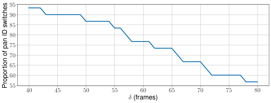
where the summation is carried out over all ground truth trajectories and is an indicator function. Consider the video number having identity switches and an IDF1 of . We plot the proportion of pan identity switches (Fig 11), that is
| (10) |
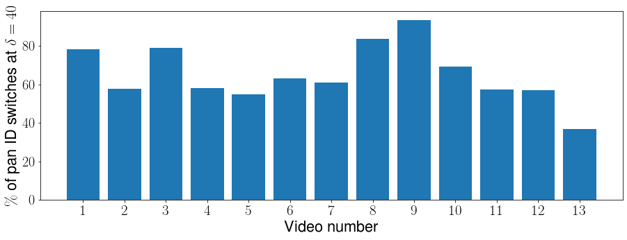
against , where varies between and frames. In video number video . From Fig. 11 it can be seen that majority of the identity switches ( at a threshold of frames) occur due to camera panning, which is the main cause of error. Visually investigating the video confirmed the statement. Fig. 10 shows the proportion of pan-identity switches for all videos at a threshold of frames. On average, pan identity switches account for of identity switches in the videos. This shows that the tracking model is able to tackle occlusions and lack of detections with the exception of extremely cluttered scenes.
IV-B Team Identification
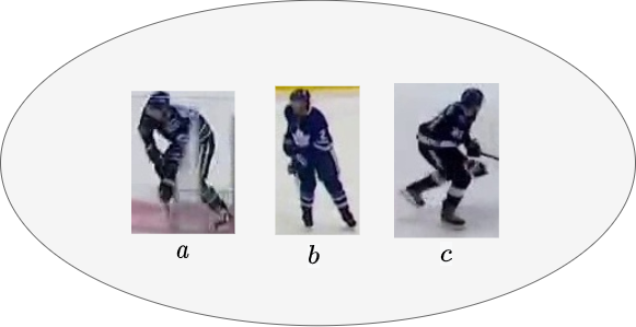
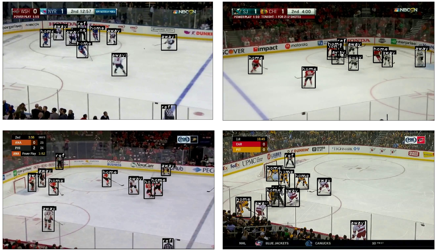
The team identification model obtains an accuracy of on the team identification test set. Table V shows the macro averaged precision, recall and F1 score for the results. The model is also able to correctly classify teams in the test set that are not present in the training set. Fig. 12 shows some qualitative results where the network is able to generalize on videos absent in training/testing data. We compare the model to color histogram features as a baseline. Each image in the dataset was cropped such that only the upper half of jersey is visible. A color histogram was obtained from the RGB representation of each image, with bins per image channel. Finally a support vector machine (SVM) with an radial basis function (RBF) kernel was trained on the normalized histogram features. The optimal SVM hyperparameters and number of histogram bins were determined using grid search by doing a five-fold cross-validation on the combination of training and validation set. The optimal hyperparameters obtained were , and . Compared to the SVM model, the deep network approach performs better on the test set demonstrating that the deep network (CNN) based approach is superior to simple handcrafted color histogram features.
IV-C Player Identification
| Method | Accuracy | Precision | Recall | F1 score |
|---|---|---|---|---|
| Proposed | ||||
| SVM with color histogram |
| Method | Accuracy | F1 score | Visiblility filtering | Postprocessing |
| Majority voting | ✓ | ✓ | ||
| Probability averaging | ||||
| Proposed w/o postprocessing | ✓ | |||
| Proposed w/o visibility filtering | ✓ | |||
| Proposed | 83.17% | 83.19% | ✓ | ✓ |
The proposed player identification network attains an accuracy of on the test set. We compare the network with Chan et al. [10] who use a secondary CNN model for aggregating probabilities on top of an CNN+LSTM model. Our proposed inference scheme, on the contrary, does not require any additional network. Since the code and dataset for Chan et al. [10] is not publicly available, we re-implemented the model by scratch and trained and evaluated the model on our dataset. The proposed network performs better than Chan et al. [10]. The network proposed by Chan et al. [10] processes shorter sequences of length 16 during training and testing, and therefore exploits less temporal context than the proposed model with sequence length 30. Also, the secondary CNN used by Chan et al. [10] for aggregating tracklet probability scores easily overfits on our dataset. Adding regularization while training the secondary CNN proposed in Chan et al. [10] on our dataset also did not improve the performance. This is because our dataset is half the size and is more skewed than the one used in Chan et al. [10], with the class consisting of half the examples in our case. The higher accuracy indicates that the proposed network and training methodology involving intelligent sampling of the class and the proposed inference scheme works better on our dataset. Additionally, temporal 1D CNNs have been reported to perform better than LSTMs in handling long range dependencies [2], which is verified by the results.
The network is able to identify digits during motion blur and unusual angles (Fig. 14). Upon inspecting the error cases, it is seen that when a two digit jersey number is misclassified, the predicted number and ground truth often share one digit. This phenomenon is observed in of misclassified two digit jersey numbers. For example, 55 is misclassified as 65 and 26 is misclassified as 28 since 6 often looks like 8 (Fig. 15) because of occlusions and folds in player jerseys.
| Accuracy | F1 score | Color | Rotation | Random cropping |
|---|---|---|---|---|
| 83.17% | 83.19% | ✓ | ✓ | ✓ |
| ✓ | ✓ | |||
| ✓ | ✓ | |||
| ✓ | ✓ |

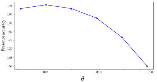
The value of (threshold for filtering out tracklets where jersey number is not visible) is determined using the validation set. In Fig 13, we plot the percentage of validation tracklets correctly classified for presence of jersey number versus the parameter . The values of tested are . The highest accuracy of at . A higher value of results in more false positives for jersey number presence. A lower than results in more false negatives. We therefore use the value of for doing inference on the test set.
IV-C1 Ablation studies
We perform ablation studies in order to study how data augmentation and inference techniques affect the player identification network performance.
Data augmentation: We perform several data augmentation techniques to boost player identification performance such data color jittering, random cropping, and random rotation by rotating each image in a tracklet by degrees. Note that since we are dealing with temporal data, these augmentation techniques are applied per tracklet instead of per tracklet-image. In this section, we investigate the contribution of each augmentation technique to the overall accuracy. Table VII shows the accuracy and weighted macro F1 score values after removing these augmentation techniques. It is observed that removing any one of the applied augmentation techniques decreases the overall accuracy and F1 score.
Inference technique: We perform an ablation study to determine how our tracklet score aggregation scheme of averaging probabilities after filtering out tracklets based on jersey number presence compares with other techniques. Recall from section III-C5 that for inference, we perform visibility filtering of tracklets and evaluate the model only on tracklets where jersey number is visible. We also include a post-processing step where only those window probability vectors are averaged for which . The other baselines tested are described:
-
1.
Majority voting: after filtering tracklets based on jersey number presence, each window probability for a tracklet is argmaxed to obtain window predictions after which a simple majority vote is taken to obtain the final prediction. For post-processing, the majority vote is only done for those window predictions with are not the class.
-
2.
Only averaging probabilities: this is equivalent to our proposed approach without visibility filtering and post-processing.
The results are shown in Table VI. We observe that our proposed aggregation technique performs the best with an accuracy of and a macro weighted F1 score of . Majority voting shows lower performance with accuracy of even after the visibility filtering and post-processing are applied. This is because majority voting does not take into account the overall window level probabilities to obtain the final prediction since it applies the argmax operation to each probability vector separately. Simple probability averaging without visibility filtering and post-processing obtains a lower accuracy demonstrating the advantage of visibility filter and post-processing step. The proposed method without the post-processing step lowers the accuracy by indicating post-processing step is of integral importance to the overall inference pipeline. The proposed inference technique without visibility filtering performs poorly when post-processing is added with an accuracy of just . This is because performing post-processing on every tracklet irrespective of jersey number visibility prevents the model to assign the class to any tracklet since the logits of the class are never taken into aggregation. Hence, tracklet filtering is an essential precursor to the post-processing step.
IV-D Overall system
We now evaluate the holistic pipeline consisting of player tracking, team identification, and player identification. This evaluation is different from evaluation done the Section 15 since the player tracklets are now obtained from the player tracking algorithm (rather than being manually annotated). The accuracy metric is the percentage of tracklets correctly classified by the algorithm.
Table VIII shows the holistic pipeline. Taking advantage of player roster improves the overall accuracy for the test videos by . For video number , the improvement in accuracy is almost . This is because the vectors and help the model focus only on the players present in the home and away roster. There are three main sources of error:
-
1.
Tracking identity switches, where the same ID is assigned to two different player tracks. These are illustrated in Fig. 16;
-
2.
Misclassification of the player’s team, as shown in Fig. 17, which causes the player jersey number probabilities to get multiplied by the incorrect roster vector; and
-
3.
Incorrect jersey number prediction by the network.
| Video number | Without roster vectors | With roster vectors |
| 1 | 95.34% | |
| 2 | 71.4% | |
| 3 | 85.9% | |
| 4 | 78.0% | |
| 5 | 81.4% | |
| 6 | ||
| 7 | 74.6% | |
| 8 | 93.75% | |
| 9 | 90.9% | |
| 10 | 88.37% | |
| 11 | 68.88% | |
| 12 | ||
| 13 | ||
| Mean | 82.8% |
V Conclusion
We have introduced and implemented an automated offline system for the challenging problem of player tracking and identification in ice hockey. The system takes as input broadcast hockey video clips from the main camera view and outputs player trajectories on screen along with their teams and identities. However, there is room for improvement. Tracking players when they leave the camera view and identifying players when their jersey number is not visible is a big challenge. In a future work, identity switches resulting from camera panning can be reduced by tracking players directly on the ice-rink coordinates using an automatic homography registration model [24]. Additionally player locations on the ice rink can be used as a feature for identifying players.
Acknowledgment
This work was supported by Stathletes through the Mitacs Accelerate Program and Natural Sciences and Engineering Research Council of Canada (NSERC). We also acknowledge Compute Canada for hardware support.
References
- [1] Omar Ajmeri and Ali Shah. Using computer vision and machine learning to automatically classify nfl game film and develop a player tracking system. In 2018 MIT Sloan Sports Analytics Conference, 2018.
- [2] Shaojie Bai, J. Zico Kolter, and Vladlen Koltun. An empirical evaluation of generic convolutional and recurrent networks for sequence modeling. arXiv:1803.01271, 2018.
- [3] Horesh Ben Shitrit, Jérôme Berclaz, François Fleuret, and Pascal Fua. Tracking multiple people under global appearance constraints. In 2011 International Conference on Computer Vision, pages 137–144, 2011.
- [4] Philipp Bergmann, Tim Meinhardt, and Laura Leal-Taixé. Tracking without bells and whistles. In The IEEE International Conference on Computer Vision (ICCV), October 2019.
- [5] Keni Bernardin and Rainer Stiefelhagen. Evaluating multiple object tracking performance: The clear mot metrics. EURASIP Journal on Image and Video Processing, 2008, 01 2008.
- [6] Alex Bewley, Zongyuan Ge, Lionel Ott, Fabio Ramos, and Ben Upcroft. Simple online and realtime tracking. In 2016 IEEE International Conference on Image Processing (ICIP), pages 3464–3468, 2016.
- [7] Alina Bialkowski, Patrick Lucey, Peter Carr, Sridha Sridharan, and Iain Matthews. Representing team behaviours from noisy data using player role. Computer Vision in Sports, pages 247–269, 2014.
- [8] Guillem Braso and Laura Leal-Taixe. Learning a neural solver for multiple object tracking. In Proceedings of the IEEE/CVF Conference on Computer Vision and Pattern Recognition (CVPR), June 2020.
- [9] Yizheng Cai, Nando de Freitas, and James J. Little. Robust visual tracking for multiple targets. In Aleš Leonardis, Horst Bischof, and Axel Pinz, editors, Computer Vision – ECCV 2006, pages 107–118, Berlin, Heidelberg, 2006. Springer Berlin Heidelberg.
- [10] Alvin Chan, Martin D. Levine, and Mehrsan Javan. Player identification in hockey broadcast videos. Expert Systems with Applications, 165:113891, 2021.
- [11] Jia Deng, Wei Dong, Richard Socher, Li-Jia Li, Kai Li, and Li Fei-Fei. Imagenet: A large-scale hierarchical image database. In 2009 IEEE Conference on Computer Vision and Pattern Recognition, pages 248–255. IEEE, 2009.
- [12] J. Donahue, L. Hendricks, S. Guadarrama, M. Rohrbach, S. Venugopalan, T. Darrell, and K. Saenko. Long-term recurrent convolutional networks for visual recognition and description. In 2015 IEEE Conference on Computer Vision and Pattern Recognition (CVPR), pages 2625–2634, Los Alamitos, CA, USA, jun 2015. IEEE Computer Society.
- [13] Tiziana D’Orazio, Marco Leo, Paolo Spagnolo, Pier Luigi Mazzeo, Nicola Mosca, Massimiliano Nitti, and Arcangelo Distante. An investigation into the feasibility of real-time soccer offside detection from a multiple camera system. IEEE Transactions on Circuits and Systems for Video Technology, 19(12):1804–1818, 2009.
- [14] S. Gerke, K. Müller, and R. Schäfer. Soccer jersey number recognition using convolutional neural networks. In 2015 IEEE International Conference on Computer Vision Workshop (ICCVW), pages 734–741, 2015.
- [15] Sebastian Gerke, Antje Linnemann, and Karsten Müller. Soccer player recognition using spatial constellation features and jersey number recognition. Computer Vision and Image Understanding, 159:105 – 115, 2017. Computer Vision in Sports.
- [16] Tianxiao Guo, Kuan Tao, Qingrui Hu, and Yanfei Shen. Detection of ice hockey players and teams via a two-phase cascaded cnn model. IEEE Access, 8:195062–195073, 2020.
- [17] Tianxiao Guo, Kuan Tao, Qingrui Hu, and Yanfei Shen. Detection of ice hockey players and teams via a two-phase cascaded cnn model. IEEE Access, 8:195062–195073, 2020.
- [18] Kaiming He, Xiangyu Zhang, Shaoqing Ren, and Jian Sun. Deep residual learning for image recognition. In 2016 IEEE Conference on Computer Vision and Pattern Recognition (CVPR), pages 770–778, 2016.
- [19] Sepp Hochreiter and Jürgen Schmidhuber. Long short-term memory. Neural Comput., 9(8):1735–1780, November 1997.
- [20] Samuel Hurault, Coloma Ballester, and Gloria Haro. Self-supervised small soccer player detection and tracking. In Proceedings of the 3rd International Workshop on Multimedia Content Analysis in Sports, MMSports ’20, page 9–18, New York, NY, USA, 2020. Association for Computing Machinery.
- [21] IIHF. Survey of Players, 2018. Available online: https://www.iihf.com/en/static/5324/survey-of-players.
- [22] Maxime Istasse, Julien Moreau, and Christophe De Vleeschouwer. Associative embedding for team discrimination. In Proceedings of the IEEE/CVF Conference on Computer Vision and Pattern Recognition (CVPR) Workshops, June 2019.
- [23] Zdravko Ivankovic, Milos Rackovic, and Miodrag Ivkovic. Automatic player position detection in basketball games. Multimedia Tools and Applications, 72:2741–2767, 10 2014.
- [24] Wei Jiang, Juan Camilo Gamboa Higuera, Baptiste Angles, Weiwei Sun, Mehrsan Javan, and Kwang Moo Yi. Optimizing through learned errors for accurate sports field registration. In 2020 IEEE Winter Conference on Applications of Computer Vision (WACV). IEEE, 2020.
- [25] Maria Koshkina, Hemanth Pidaparthy, and James H. Elder. Contrastive learning for sports video: Unsupervised player classification. In Proceedings of the IEEE/CVF Conference on Computer Vision and Pattern Recognition (CVPR) Workshops, pages 4528–4536, June 2021.
- [26] G. Li, S. Xu, X. Liu, L. Li, and C. Wang. Jersey number recognition with semi-supervised spatial transformer network. In 2018 IEEE/CVF Conference on Computer Vision and Pattern Recognition Workshops (CVPRW), pages 1864–18647, 2018.
- [27] Tsung-Yi Lin, Piotr Dollár, Ross Girshick, Kaiming He, Bharath Hariharan, and Serge Belongie. Feature pyramid networks for object detection. In 2017 IEEE Conference on Computer Vision and Pattern Recognition (CVPR), pages 936–944, 2017.
- [28] Tsung-Yi Lin, Michael Maire, Serge Belongie, James Hays, Pietro Perona, Deva Ramanan, Piotr Dollár, and C. Lawrence Zitnick. Microsoft : Common objects in context. In David Fleet, Tomas Pajdla, Bernt Schiele, and Tinne Tuytelaars, editors, Computer Vision – ECCV 2014, pages 740–755, Cham, 2014. Springer International Publishing.
- [29] H. Liu and B. Bhanu. Pose-guided R-CNN for jersey number recognition in sports. In 2019 IEEE/CVF Conference on Computer Vision and Pattern Recognition Workshops (CVPRW), pages 2457–2466, 2019.
- [30] Jingchen Liu and Peter Carr. Detecting and tracking sports players with random forests and context-conditioned motion models. Computer Vision in Sports, pages 113–132, 2014.
- [31] W. Lu, J. Ting, J. J. Little, and K. P. Murphy. Learning to track and identify players from broadcast sports videos. IEEE Transactions on Pattern Analysis and Machine Intelligence, 35(7):1704–1716, July 2013.
- [32] Wei-Lwun Lu, Jo-Anne Ting, James J. Little, and Kevin P. Murphy. Learning to track and identify players from broadcast sports videos. IEEE Transactions on Pattern Analysis and Machine Intelligence, 35(7):1704–1716, 2013.
- [33] Fernando Martello. Uniforms for the NHL team, April 2020. Available at https://commons.wikimedia.org/wiki/File:Montreal_canadiens_unif.png.
- [34] P. L. Mazzeo, P. Spagnolo, M. Leo, and T. D’Orazio. Visual players detection and tracking in soccer matches. In 2008 IEEE Fifth International Conference on Advanced Video and Signal Based Surveillance, 2008.
- [35] Kenji Okuma, Ali Taleghani, Nando de Freitas, James J. Little, and David G. Lowe. A boosted particle filter: Multitarget detection and tracking. In Tomás Pajdla and Jiří Matas, editors, Computer Vision - ECCV 2004, pages 28–39, Berlin, Heidelberg, 2004. Springer Berlin Heidelberg.
- [36] Joseph Redmon, Santosh Divvala, Ross Girshick, and Ali Farhadi. You only look once: Unified, real-time object detection. In 2016 IEEE Conference on Computer Vision and Pattern Recognition (CVPR), pages 779–788, 2016.
- [37] Shaoqing Ren, Kaiming He, Ross Girshick, and Jian Sun. Faster r-cnn: Towards real-time object detection with region proposal networks. In C. Cortes, N. Lawrence, D. Lee, M. Sugiyama, and R. Garnett, editors, Advances in Neural Information Processing Systems, volume 28. Curran Associates, Inc., 2015.
- [38] Ergys Ristani, Francesco Solera, Roger Zou, Rita Cucchiara, and Carlo Tomasi. Performance measures and a data set for multi-target, multi-camera tracking. In Gang Hua and Hervé Jégou, editors, Computer Vision – ECCV 2016 Workshops, pages 17–35, Cham, 2016. Springer International Publishing.
- [39] Ryan Sanford, Siavash Gorji, Luiz G. Hafemann, Bahareh Pourbabaee, and Mehrsan Javan. Group activity detection from trajectory and video data in soccer. In Proceedings of the IEEE/CVF Conference on Computer Vision and Pattern Recognition (CVPR) Workshops, June 2020.
- [40] Adrià Arbués Sangüesa, C. Ballester, and G. Haro. Single-camera basketball tracker through pose and semantic feature fusion. ArXiv, abs/1906.02042, 2019.
- [41] Arda Senocak, Tae-Hyun Oh, Junsik Kim, and In So Kweon. Part-based player identification using deep convolutional representation and multi-scale pooling. In Proceedings of the IEEE Conference on Computer Vision and Pattern Recognition (CVPR) Workshops, June 2018.
- [42] S. Tang, M. Andriluka, B. Andres, and B. Schiele. Multiple people tracking by lifted multicut and person re-identification. In 2017 IEEE Conference on Computer Vision and Pattern Recognition (CVPR), pages 3701–3710, July 2017.
- [43] Rajkumar Theagarajan and Bir Bhanu. An automated system for generating tactical performance statistics for individual soccer players from videos. IEEE Transactions on Circuits and Systems for Video Technology, 31(2):632–646, 2021.
- [44] Xiaofeng Tong, Jia Liu, Tao Wang, and Yimin Zhang. Automatic player labeling, tracking and field registration and trajectory mapping in broadcast soccer video. ACM Trans. Intell. Syst. Technol., 2(2), February 2011.
- [45] Kanav Vats, Mehrnaz Fani, David A. Clausi, and John Zelek. Multi-task learning for jersey number recognition in ice hockey. In Proceedings of the 4th International Workshop on Multimedia Content Analysis in Sports, MMSports’21, page 11–15, New York, NY, USA, 2021. Association for Computing Machinery.
- [46] Kanav Vats, Mehrnaz Fani, David A. Clausi, and John Zelek. Puck localization and multi-task event recognition in broadcast hockey videos. In Proceedings of the IEEE/CVF Conference on Computer Vision and Pattern Recognition (CVPR) Workshops, pages 4567–4575, June 2021.
- [47] Kanav Vats, Mehrnaz Fani, Pascale Walters, David A. Clausi, and John Zelek. Event detection in coarsely annotated sports videos via parallel multi-receptive field 1d convolutions. In Proceedings of the IEEE/CVF Conference on Computer Vision and Pattern Recognition (CVPR) Workshops, June 2020.
- [48] Vermaak, Doucet, and Perez. Maintaining multimodality through mixture tracking. In Proceedings Ninth IEEE International Conference on Computer Vision, pages 1110–1116 vol.2, Oct 2003.
- [49] P. Viola and M. Jones. Rapid object detection using a boosted cascade of simple features. In Proceedings of the 2001 IEEE Computer Society Conference on Computer Vision and Pattern Recognition. CVPR 2001, volume 1, pages I–I, Dec 2001.
- [50] Nicolai Wojke, Alex Bewley, and Dietrich Paulus. Simple online and realtime tracking with a deep association metric. In 2017 IEEE International Conference on Image Processing (ICIP), pages 3645–3649. IEEE, 2017.
- [51] Ruiheng Zhang, Lingxiang Wu, Yukun Yang, Wanneng Wu, Yueqiang Chen, and Min Xu. Multi-camera multi-player tracking with deep player identification in sports video. Pattern Recognition, 102:107260, 2020.
- [52] Yifu Zhang, Chunyu Wang, Xinggang Wang, Wenjun Zeng, and Wenyu Liu. Fairmot: On the fairness of detection and re-identification in multiple object tracking. arXiv preprint arXiv:2004.01888, 2020.
- [53] Matko Šaric, Hrvoje Dujmic, Vladan Papic, and Nikola Rožic. Player number localization and recognition in soccer video using hsv color space and internal contours. International Journal of Electrical and Computer Engineering, 2(7):1408 – 1412, 2008.