FedTune: Automatic Tuning of Federated Learning Hyper-Parameters from System Perspective

Abstract

In Federated Learning (FL), hyper-parameters significantly affect the training overhead in terms of computation time, transmission time, computation load, and transmission load. The current practice of manually selecting FL hyper-parameters puts a high burden on FL practitioners since various applications have different training preferences. In this paper, we propose FedTune, an automatic hyper-parameter tuning algorithm tailored to applications’ diverse system requirements in FL training. FedTune is lightweight and flexible, achieving 8.48%-26.75% improvement for different datasets compared to using fixed FL hyper-parameters.

I Introduction

Federated learning (FL) has been applied to a wide range of applications such as mobile keyboard [4] and speech recognition [17] on top of mobile devices [1] and Internet of Things (IoT) [26, 27]. Compared to other model training paradigms (e.g., centralized machine learning [6], conventional distributed machine learning [20]), FL has unique properties such as massively distributed, significant unbalanced, and non-IID data distribution [15]. In addition to the common hyper-parameters of model training such as learning rates, optimizers, and mini-batch sizes, FL has unique hyper-parameters, including aggregation algorithms and participant selection [10, 11]. Fortunately, these FL hyper-parameters do not affect the FL convergence property. Many FL algorithms such as FedAvg [15], have been proved to converge to the global optimum under different FL hyper-parameters [14][22]. However, they can significantly affect the training overhead of reaching the final model.

In this paper, we focus on the training overhead. Specifically, computation time (CompT), transmission time (TransT), computation load (CompL), and transmission load (TransL) are the four most important system overhead. CompT measures how long an FL system spends in model training; TransT represents how long an FL system spends in model parameter transmission between the clients and the server; CompL is the number of Floating-Point Operation (FLOP) that an FL system consumes; and TransL is the total data size transmitted between the clients and the server.

Application scenarios can have different training preferences in terms of CompT, TransT, CompL, and TransL. Consider the following examples: (1) attack and anomaly detection in computer networks [3] is time-sensitive (CompT and TransT) as it needs to adapt to malicious traffic rapidly; (2) smart home control systems for indoor environment automation [16], e.g., heating, ventilation, and air conditioning (HVAC), are sensitive to computation (CompT and CompL) because sensor devices are limited in computation capabilities; (3) traffic monitoring systems for vehicles [24] are communication-sensitive (TransT and TransL) because cellular communications are usually adopted to provide city-scale connectivity.

A few papers have studied FL training performance under different hyper-parameters [21]. However, they do not consider CompT, TransT, CompL, and TransL together, which are essential from the system’s perspective. In addition, it is challenging to tune multiple hyper-parameters in order to achieve diverse training preferences, especially when we need to optimize multiple system aspects. For example, it is unclear how to select hyper-parameters to build an FL training solution that is both CompT and TransL-efficient.

Contributions. This paper targets a new research problem of optimizing the hyper-parameters for FL from the system perspective. To do so, we formulate the system overhead in FL training and conduct extensive measurements to understand FL training performance. To avoid manual hyper-parameter selection, we propose FedTune, an algorithm that automatically tunes FL hyper-parameters during model training, respecting application training preferences. Our evaluation results show that FedTune achieves a promising performance in reducing the system overhead.

II Related Work

Hyper-Parameter Optimization (HPO) is a field that has been extensively studied [25]. Many classical HPO algorithms, e.g., Bayesian optimization [19], successive halving [7], and hyperband [12], are designed to optimize hyper-parameters of machine learning models.

Designing HPO methods for FL, however, is a new research area. Only a few works have touched FL HPO problems. For example, FedEx is a general framework to optimize the round-to-accuracy of FL by exploiting the Neural Architecture Search (NAS) techniques of weight-sharing, which improves the baseline by several percentage points [8]; FLoRA determines the global hyper-parameters by selecting the hyper-parameters that have good performances in local clients [28]. However, existing works cannot be directly applied to our scenario of optimizing FL hyper-parameter for different FL training preferences for two reasons. First, CompT (in seconds), TransL (in seconds), CompL (in FLOPs), and TransL (in bytes) are not comparable with each other. Incorporating training preferences in HPO is not trivial. Second, hyper-parameter tuning needs to be done during the FL training. No “comeback” is allowed as the FL model keeps training until its final model accuracy. Otherwise, it will cause significantly more system overhead.

III Understanding the Problem

We first quantify the system overheads of FedAvg to illustrate the problem. FedAvg minimizes the following objective

$$f(w)=\sum_{k=1}^{K}\frac{n_{k}}{n}F_{k}(w)\quad\text{where}\quad F_{k}(w)=\frac{1}{n_{k}}\sum_{i\in\mathcal{P}_{k}}f_{i}(w)$$ (1)

where $f_{i}(w)$ is the loss of the model on data point $(x_{i},y_{i})$, that is, $f_{i}(w)=\ell(x_{i},y_{i};w)$, $K$ is the total number of clients, $\mathcal{P}_{k}$ is the set of indexes of data points on client $k$, with $n_{k}=|\mathcal{P}_{k}|$, and $n$ is the total number of data points from all clients, i.e., $n=\sum_{k=1}^{K}n_{k}$. Due to the large number of clients in a typical FL application (e.g., millions of clients in the Google Gboard project [4]), a common practice is to randomly select a small fraction of clients in each training round. In the rest of this paper, we refer to the selected clients as participants and denote $M$ as the number of participants on each training round. Each participant makes $E$ training passes over its local data in each round before uploading its model parameters to the server for aggregation. Afterward, participants wait to receive an updated global model from the server, and a new training round starts.

III-A System Model

Assume that clients are homogeneous in terms of hardware (e.g., CPU/GPU) and network (e.g., transmission speeds). Let $b_{k,r}$ indicates whether client $k$ participates at the training round $r$. Then, we have $\sum_{k=1}^{K}b_{k,r}=M$, i.e., each round selects $M$ participants. The number of training rounds to reach the final model accuracy is denoted by $R$, which is unknown a priori and varies when different sets of FL hyper-parameters are used in FL training. CompT, TransT, CompL, and TransL can be formulated as follows.

Computation Time (CompT). If client $k$ is selected on a training round, it spends time in local training. The local training delay can be represented by $C_{1}\cdot E\cdot n_{k}$, where $C_{1}$ is a constant. It is proportional to its number of data points (i.e., $n_{k}$) because $n_{k}$ decides the number of local updates (number of mini-batches) for one epoch, and each local update includes one forward-pass and one backward-pass. The computation time of the training round $r$ is determined by the slowest participant and thus is represented by $C_{1}\cdot E\cdot\max_{k=1}^{K}b_{k,r}\cdot n_{k}$. In total, the computation time of an FL training can be formulated as

$$CompT=C_{1}\cdot E\cdot\sum_{r=1}^{R}\max_{k=1}^{K}b_{k,r}\cdot n_{k}$$ (2)

Transmission Time (TransT). Each participant on a training round needs one download and one upload of model parameters from and to the server [21]. Thus, the transmission time is the same for all participants on any training round, i.e., a constant $C_{2}$. The total transmission time is represented by

$$TransT=C_{2}\cdot R$$ (3)

Computation Load (CompL). Client $k$ causes $C_{3}\cdot E\cdot n_{k}$ computation load if it is selected on a training round, where $C_{3}$ is a constant. The computation load of the training round $r$ is the summation of each participant’s computation load and thus is $C_{3}\cdot E\cdot\sum_{k=1}^{K}b_{k,r}\cdot n_{k}$. We can formulate the overall computation load as

$$CompL=C_{3}\cdot E\cdot\sum_{r=1}^{R}\sum_{k=1}^{K}b_{k,r}\cdot n_{k}$$ (4)

Transmission Load (TransL). Since each training round selects $M$ participants, the transmission load for a training round is $C_{4}\cdot M$ where $C_{4}$ is a constant. The total number of training rounds is $R$, and thus, the total transmission load of an FL training is represented by

$$TransL=C_{4}\cdot R\cdot M$$ (5)

In the experiments, we assign the model’s number of FLOPs for one input to $C_{1}$ and $C_{3}$, and the model’s number of parameters to $C_{2}$ and $C_{4}$.

III-B Measurement Study

We conduct measurements to study the system overhead when different FL hyper-parameters are used for training. We use the Google speech-to-command dataset [23]. Please refer to Section V-A for the training setup. The speech-to-command dataset meets the data properties of FL: massively distributed, unbalanced, and non-IID. The measurement study investigates the FL training overhead in terms of the following three hyper-parameters.

• The number of participants (i.e., $M$). It is well-known that more participants on each training round have a better round-to-accuracy performance [15]. In the measurement study, we set $M$ to 1, 10, 20, and 50.

• The number of training passes (i.e., $E$). Increasing the number of training passes as a method to improve communication efficiency has been adopted in several works, such as FedAvg [15] and FedNova [14]. In the measurement study, we set $E$ to 0.5, 1, 2, 4, 8, where 0.5 means that only half of each client’s local data are used for local training in each round.

• Model complexity. We also investigate how the model complexity influences the training overhead if a target accuracy is met. We use ResNet [5] to build different models, as listed in Table I.

Model	ResNet-10	ResNet-18	ResNet-26	ResNet-34
#BasicBlock	[1, 1, 1, 1]	[2, 2, 2, 2]	[3, 3, 3, 3]	[3, 4, 6, 3]
#FLOP ($\times 10^{6}$)	12.5	26.8	41.1	60.1
#Params ($\times 10^{3}$)	79.7	177.2	274.6	515.6
Accuracy	0.88	0.90	0.90	0.92

TABLE I: Different models used for the measurement study.

Computation Time (CompT). Fig. 1(a) compares CompT for a different number of participants $M$ and a different number of training passes $E$. In the experiments, we use ResNet-18 and normalize their overheads. As we can see, more participants lead to smaller CompT, i.e., it takes a shorter time to converge. However, the difference is not significant among 10, 20, and 50 participants, especially when the number of training passes is large. In addition, we can see that larger $E$ has worse CompT.

Transmission Time (TransT). Fig. 1(b) plots TransT, which clearly shows that TransT favors larger $M$ and $E$. Since TransT is dependent on the number of training rounds $R$ (Eq. (3)), it is equivalent to the metric of round-to-accuracy. Our measurement result is consistent with the common knowledge (e.g., [22]) that more participants and more training passes have a better round-to-accuracy performance. We can also observe that when $M$ is small, e.g., 1, TransL is much worse than the other cases.

Computation Load (CompL). Fig. 1(c) shows CompL. We make the following observations: (1) More participants result in worse CompL. The results indicate that the gain of faster model convergence from more participants does not compensate for the higher computation costs introduced by more participants. (2) CompL is increased when more training passes are used. This is probably because that larger $E$ diverges the model training [13] and thus, the data utility per unit of computation cost is reduced.

Transmission Load (TransL). Fig. 1(d) illustrates TransL. As shown, more participants greatly increase TransL. This is because more participants can only weakly reduce the number of training rounds $R$ [14], however, in each round, the number of transmissions is linearly increased with the number of participants. Regarding the number of training passes, larger $E$ reduces the total number of training rounds $R$ and thus has better TransL. On the other hand, the gain of larger $E$ is diminishing. The results are consistent with the analysis of [14] that $R$ is hyperbolic with $E$ (the turning point happens around 100-1000 in their experiments).

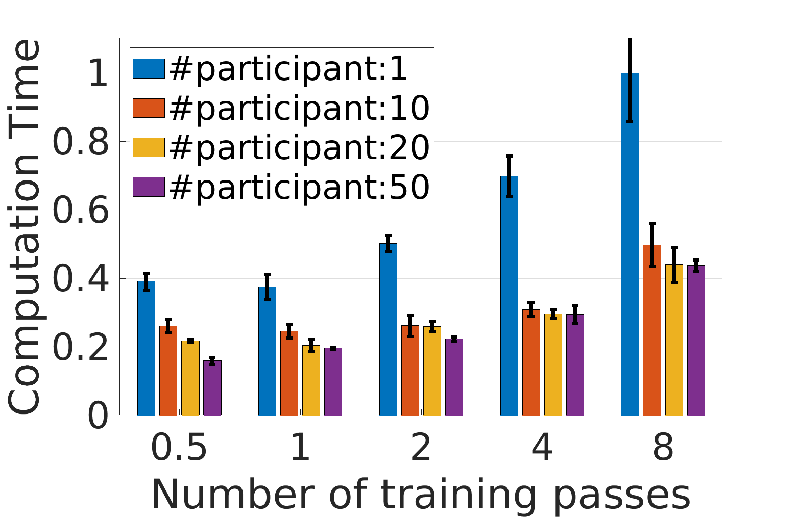
(a) Computation Time

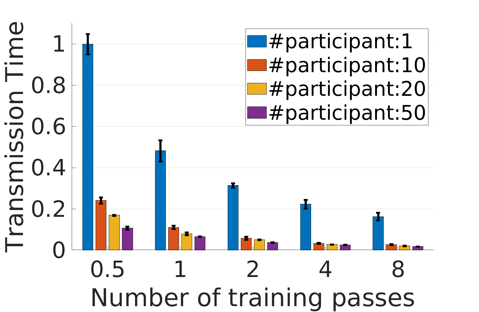
(b) Transmission Time

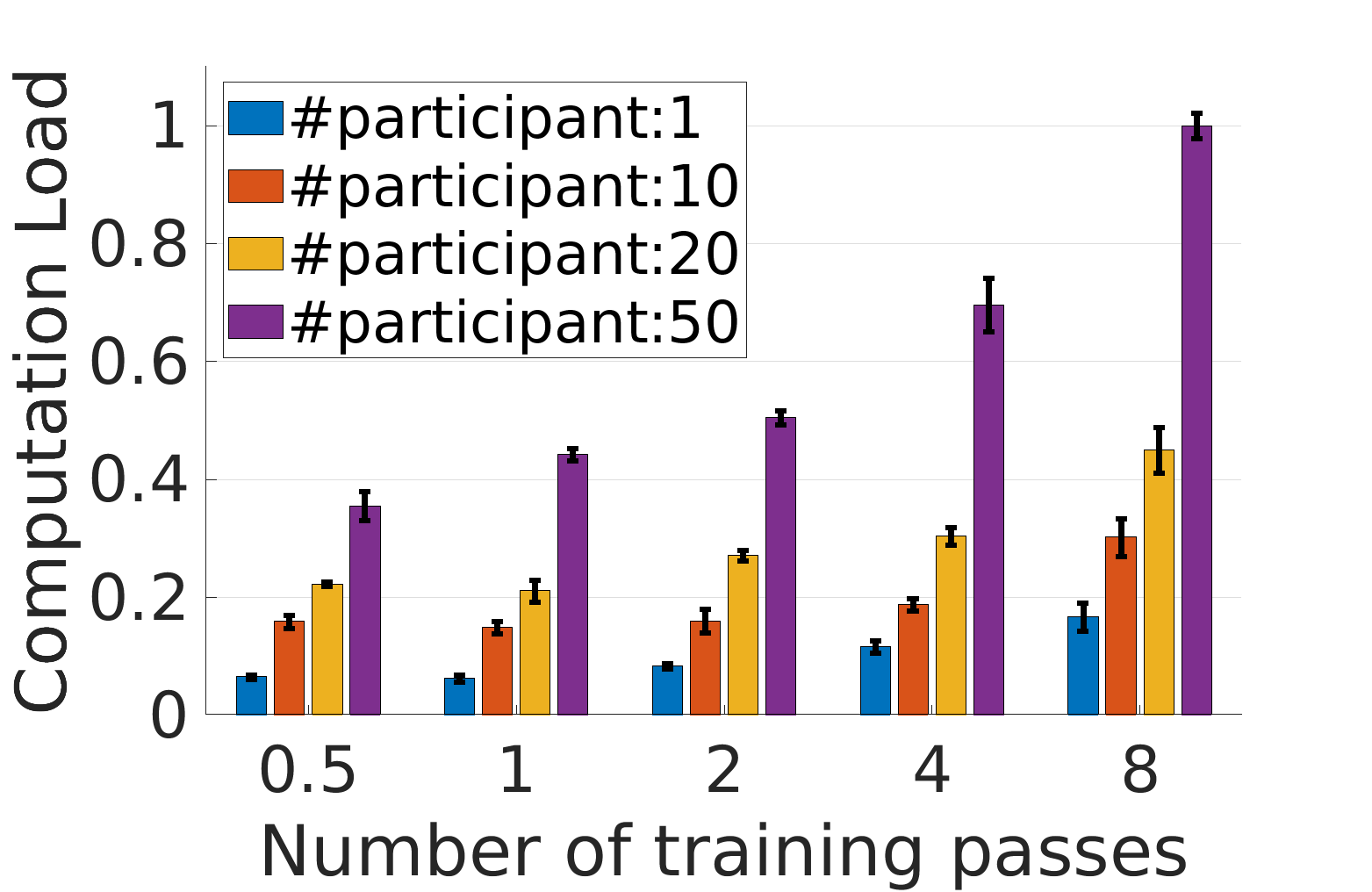
(c) Computation Load

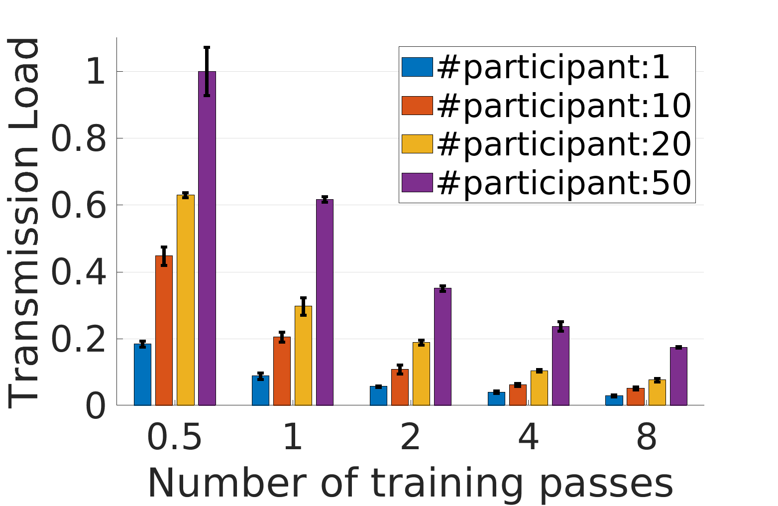
(d) Transmission Load

Figure 1: CompT, TransT, CompL, and TransL when a different number of participants and a different number of training passes are used. The lower the better.

Model Complexity. Table I tabulates the models for comparing training overheads versus model complexity. In this experiment, we select one participant ($M=1$) to train one pass ($E=1$) on each training round. Fig. 2 shows the normalized CompT, TransT, CompL, and TransL for different models. The x-axis is the target model accuracy, and the y-axis is the corresponding overhead to reach that model accuracy. Since only one client and one training pass are used on each round, CompT and CompL have the same normalized comparison, and so are TransT and TransL. The results show that smaller models are better with regard to all training aspects. In addition, it is interesting to note that heavier models have higher increase rates of overhead versus model accuracy. This means that model selection is especially essential for high model accuracy applications.

III-C Summary of System Overheads

Based on our measurement study, we summarize systems overheads versus FL hyper-parameters in Table II. As we can see, CompT, TransT, CompL, and TransL conflict with each other in terms of $M$ and $E$. Regarding model complexity, smaller models have better system overhead if the model accuracy is satisfied. Please note that Table II is consistent with existing works (e.g., [22]), but is more comprehensive.

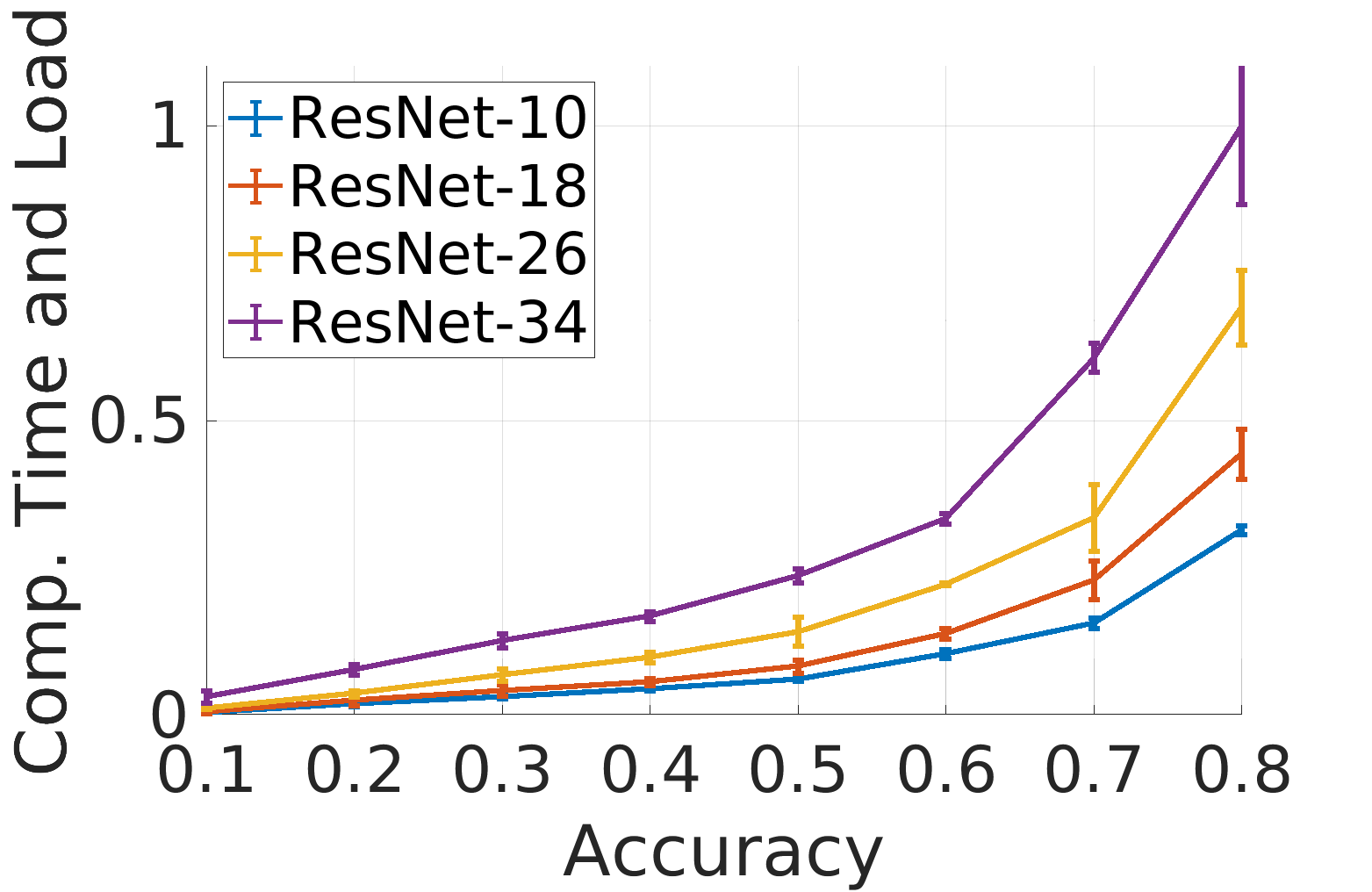
(a) Computation time and load

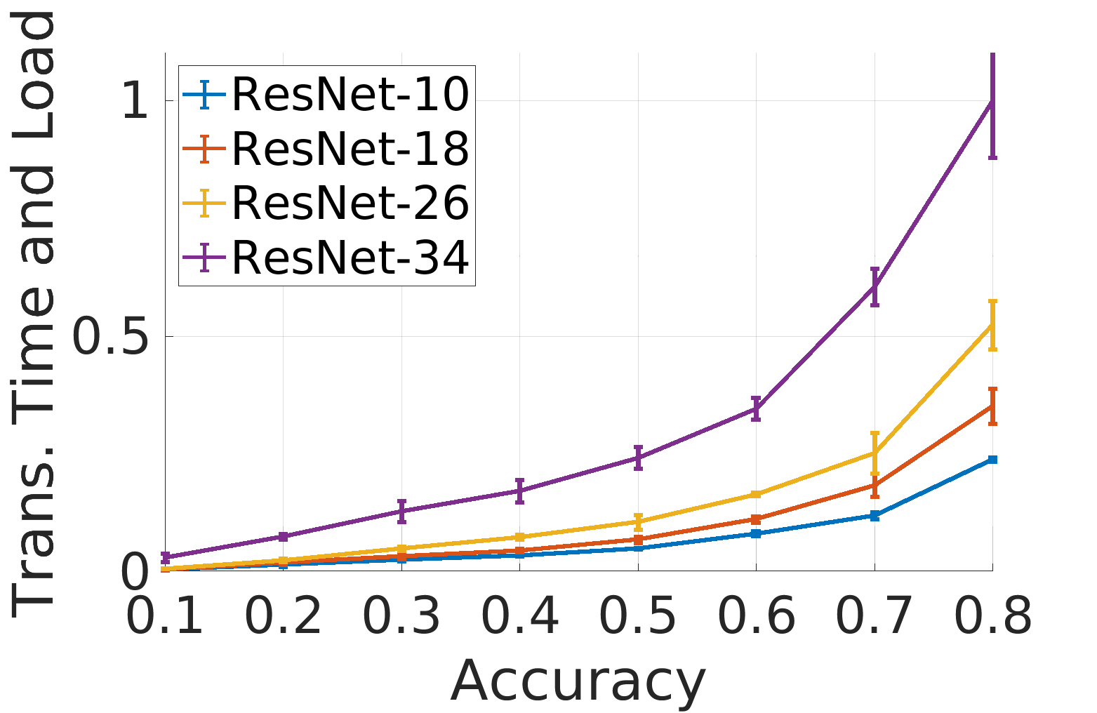
(b) Transmission time and load

Figure 2: CompT, TransT, CompL, and TransL versus model complexity. The lower the better.

IV FedTune

Training aspect $M$ $E$ Model complexity CompT $>$ $<$ $<$ TransT $>$ $>$ $<$ CompL $<$ $<$ $<$ TransL $<$ $>$ $<$ Model Accuracy $=$ $=$ $>$

TABLE II: System overheads versus the number of participants $M$, the number of training passes $E$, and model complexity. ‘$<$’, ‘$=$’, and ‘$>$’ means the smaller the better, does not matter, and the larger the better, respectively.

FedTune considers training preferences for CompT, TransT, CompL, and TransL, denoted by $\alpha$, $\beta$, $\gamma$, and $\delta$, respectively. We have $\alpha+\beta+\gamma+\delta=1$. For example, $\alpha=0.6$, $\beta=0.2$, $\gamma=0.1$, and $\delta=0.1$ represent that the application is greatly concerned about CompT, while slightly about TransT, with CompL and TransL the least concern.

IV-A Problem Formulation

For two sets of FL hyper-parameters $S_{1}$ and $S_{2}$, FedTune defines the comparison function $I(S_{1},S_{2})$ as

$$I(S_{1},S_{2})=\alpha\times\frac{t_{2}-t_{1}}{t_{1}}+\beta\times\frac{q_{2}-q_{1}}{q_{1}}$$ (6)

$$+\gamma\times\frac{z_{2}-z_{1}}{z_{1}}+\delta\times\frac{v_{2}-v_{1}}{v_{1}}$$

where $t_{1}$ and $t_{2}$ are CompT for $S_{1}$ and $S_{2}$ achieving the same model accuracy. Correspondingly, $q_{1}$ and $q_{2}$ are TransT, $z_{1}$ and $z_{2}$ are CompL, and $v_{1}$ and $v_{2}$ are TransL. If $I(S_{1},S_{2})<0$, then $S_{2}$ is better than $S_{1}$. A set of hyper-parameters is better than another set if the weighted improvement of some training aspects (e.g., CompT and CompL) is higher than the weighted degradation of the remaining training aspects (e.g., TransT and TransL). The weights are training preferences on CompT, TransT, CompL, and TransL.

However, the training overhead for different sets of FL hyper-parameters are unknown a priori. As a result, directly identifying the optimal hyper-parameters before FL training is impossible. Instead, we propose an iterative method to optimize the next set of hyper-parameters. Given the current set of hyper-parameters $S_{cur}$, the goal is to find a set of hyper-parameters $S_{nxt}$ that improves the training performance the most, that is, minimizing the following objective function:

$$G(S_{nxt})=\alpha\times\frac{t_{nxt}-t_{cur}}{t_{cur}}+\beta\times\frac{q_{nxt}-q_{cur}}{q_{cur}}$$ (7)

$$+\gamma\times\frac{z_{nxt}-z_{cur}}{z_{cur}}+\delta\times\frac{v_{nxt}-v_{cur}}{v_{cur}}$$

where $t_{cur}$, $q_{cur}$, $z_{cur}$, and $v_{cur}$ are CompT, TransT, CompL, and TransL under the current hyper-parameters $S_{cur}$; $t_{nxt}$, $q_{nxt}$, $z_{nxt}$, and $v_{nxt}$ are CompT, TransT, CompL, and TransL for the next hyper-parameters $S_{nxt}$. We focus on the number of participants $M$ and the number of training passes $E$, since model complexity is monotonous with training overheads. Therefor, we need to optimize $S_{nxt}=\{M_{nxt},E_{nxt}\}$.

IV-B $S_{nxt}$ Optimization

To find the optimal $S_{nxt}$, we take the derivatives of $G(S_{nxt})$ over $M$ and $E$, obtaining

$$\Delta M=\frac{\partial G(S_{nxt})}{\partial M}=\frac{\alpha}{t_{cur}}\times\frac{\partial t_{nxt}}{\partial M}+\frac{\beta}{q_{cur}}\times\frac{\partial q_{nxt}}{\partial M}$$ (8)

$$+\frac{\gamma}{z_{cur}}\times\frac{\partial z_{nxt}}{\partial M}+\frac{\delta}{v_{cur}}\times\frac{\partial v_{nxt}}{\partial M}$$

$$\Delta E=\frac{\partial G(S_{nxt})}{\partial E}=\frac{\alpha}{t_{cur}}\times\frac{\partial t_{nxt}}{\partial E}+\frac{\beta}{q_{cur}}\times\frac{\partial q_{nxt}}{\partial E}$$ (9)

$$+\frac{\gamma}{z_{cur}}\times\frac{\partial z_{nxt}}{\partial E}+\frac{\delta}{v_{cur}}\times\frac{\partial v_{nxt}}{\partial E}$$

We illustrate how to obtain $\Delta M$. The process of solving $\Delta E$ is similar. Considering that each step makes a small adjustment of $M$, $\partial t_{nxt}/\partial M$ can be represented by $(+1)\times|t_{nxt}-t_{cur}|$, where $(+1)$ means CompT prefers larger $M$ according to Table II. To estimate $|t_{nxt}-t_{cur}|$, we apply a linear function $\eta_{t-1}\times|t_{cur}-t_{prv}|$ where $\eta_{t-1}=\frac{|t_{cur}-t_{prv}|}{|t_{prv}-t_{prvprv}|}$ ($t_{prvprv}$ is the CompT at two steps before). Similarly, we have $\eta_{q-1}$, $\eta_{z-1}$, $\eta_{v-1}$ for TransT, CompL, and TransL when calculating their derivatives over $M$. As a result, $\Delta M$ can be approximated as

$$\Delta M=\frac{(+1)\times\alpha\times\eta_{t-1}\times|t_{cur}-t_{prv}|}{t_{cur}}$$ (10)

$$+\frac{(+1)\times\beta\times\eta_{q-1}\times|q_{cur}-q_{prv}|}{q_{cur}}$$

$$+\frac{(-1)\times\gamma\times\eta_{z-1}\times|z_{cur}-z_{prv}|}{z_{cur}}$$

$$+\frac{(-1)\times\delta\times\eta_{v-1}\times|v_{cur}-v_{prv}|}{v_{cur}}$$

Similarly, we can calculate $\Delta E$ as

$$\Delta E=\frac{(-1)\times\alpha\times\zeta_{t-1}\times|t_{cur}-t_{prv}|}{t_{cur}}$$ (11)

$$+\frac{(+1)\times\beta\times\zeta_{q-1}\times|q_{cur}-q_{prv}|}{q_{cur}}$$

$$+\frac{(-1)\times\gamma\times\zeta_{z-1}\times|z_{cur}-z_{prv}|}{z_{cur}}$$

$$+\frac{(+1)\times\delta\times\zeta_{v-1}\times|v_{cur}-v_{prv}|}{v_{cur}}$$

where $\zeta_{t-1}$, $\zeta_{q-1}$, $\zeta_{z-1}$, and $\zeta_{v-1}$ are the parameters for calculating the derivatives of CompT, TransT, CompL, and TransL over $E$.

IV-C Decision Making and Parameter Update

FedTune is activated when the model accuracy is improved by at least $\epsilon$. Then, it computes $\Delta M$ and $\Delta E$, and determines the next $M$ and $E$ based on the signs of $\Delta M$ and $\Delta E$. Specifically, $M_{nxt}=M_{cur}+1$ if $\Delta M>0$, otherwise, $M_{nxt}=M_{cur}-1$. Likewise, FedTune increases $E_{nxt}$ by one if $\Delta E>0$; else FedTune decreases $E_{nxt}$ by one. The FL training is resumed using the new hyper-parameters. FedTune is lightweight and negligible to the FL training: it only requires dozens of multiplication and addition calculations.

FedTune automatically updates $\eta_{t-1}$, $\eta_{q-1}$, $\eta_{z-1}$, $\eta_{v-1}$, $\zeta_{t-1}$, $\zeta_{q-1}$, $\zeta_{z-1}$, and $\zeta_{v-1}$ during FL training. At each step, FedTune updates the parameters that favor the current decision. For example, if $M_{cur}$ is larger than $M_{prv}$, FedTune updates $\eta_{t-1}$ and $\eta_{q-1}$ as CompT and TransT prefer larger $M$; otherwise, FedTune updates $\eta_{z-1}$ and $\eta_{v-1}$.

Furthermore, FedTune incorporates a penalty mechanism to mitigate bad decisions. Given the previous hyper-parameters $S_{prv}$ and the current hyper-parameters $S_{cur}$, FedTune calculates the comparison function $I(S_{prv},S_{cur})$. A bad decision occurs if the sign of $I(S_{prv},S_{cur})$ is positive. In this case, FedTune multiplies the parameters that are against the current decision by a constant penalty factor, denoted by $D$ ($D\geq 1$). For example, if $I(S_{prv},S_{cur})>0$ and $M_{cur}>M_{prv}$, FedTune updates $\eta_{t-1}$ and $\eta_{q-1}$ as explained before, but also multiplies $\eta_{z-1}$ and $\eta_{v-1}$ by $D$.

V Experiments and Analysis

Benchmarks and Baseline. We evaluate FedTune on three datasets: speech-to-command [23], EMNIST [2], and Cifar-100 [9], and three aggregation methods: FedAvg [15], FedNova [22], and FedAdagrad [18]. We set equal values for the combination of training preferences $\alpha$, $\beta$, $\gamma$ and $\delta$ (see the first column in Table V). Therefore, for each dataset, we conduct 15 combinations of training preferences. We set target model accuracy for each dataset and measure CompT, TransT, CompL, and TransL for reaching the target model accuracy. We regard the practice of using fixed $M$ and $E$ as the baseline and compare FedTune to the baseline by calculating Eq. (6). We implemented FedTune in PyTorch. All the experiments are conducted on a server with 24-GB Nvidia RTX A5000 GPUs.

V-A Overall Performance

Dataset Speech-command EMNIST Cifar-100 Data Feature Voice Handwriting Image ML Model ResNet-10 2-layer MLP ResNet-10 Performance +22.48% (17.97%) +8.48% (5.51%) +9.33% (5.47%)

TABLE III: Performance of FedTune for diverse datasets when FedAvg aggregation method is applied.

Training setup. (1) speech-to-command dataset. It classifies audio clips to 35 commands (e.g., ‘yes’, ‘off’). We transform audio clips to 64-by-64 spectrograms and then downsize them to 32-by-32 gray-scale images. As officially suggested [23], we use 2112 clients’ data for training and the remaining 506 clients’ data for testing. We set the mini-batch size to 5, considering that many clients have few data points. We use ResNet-10 and the target model accuracy of 0.8. (2) EMNIST dataset. It classifies handwriting (28-by-28 gray-scale images) into 62 digits and letters (lowercase and uppercase). We split the dataset based on the writer ID. We randomly select 70% writers’ data for training and the remaining for testing. We use a Multiplayer Perception (MLP) model with one hidden layer (200 neurons with ReLu activation). We set the mini-batch size to 10 and the target model accuracy of 0.7. (3) Cifar-100 dataset. It classifies 32-by-32 RGB images to 100 classes. We randomly split the dataset into 1200 users, where each user has 50 data points. Then, we randomly select 1000 users for training and the remaining 200 users for testing. We set the mini-batch size to 10. ResNet-18 is used, and the target model accuracy is set to 0.2 (due to our limited computational capability, we set a low threshold for Cifar-100).

For all datasets, we normalize the input images with the mean and the standard deviation of the training data before feeding them to models for training and testing. Both $M$ and $E$ are initially set to 20. FedTune is activated when the model accuracy is increased by at least 0.01 (i.e., $\epsilon=0.01$). The penalty factor $D$ is set to 10. All results are averaged by three experiments.

Aggregator FedAvg FedNova FedAdagrad Performance +22.48% (17.97%) +23.53% (6.64%) +26.75% (6.10%)

TABLE IV: Performance of FedTune for diverse aggregation algorithms. Speech-to-command dataset and ResNet-10 are used in this experiment.

$\alpha$ $\beta$ $\gamma$ $\delta$ CompT ($10^{12}$) TransT ($10^{6}$) CompL ($10^{12}$) TransL ($10^{6}$) Final M Final E Overall - - - - 0.94 (0.01) 11.61 (0.10) 5.97 (0.04) 232.24 (1.99) 20 20 - 1.0 0.0 0.0 0.0 0.42 (0.02) 50.19 (2.57) 4.57 (0.22) 2418.71 (240.91) 57.33 (4.50) 1.00 (0.00) +55.23% (2.22%) 0.0 1.0 0.0 0.0 1.34 (0.22) 7.68 (1.12) 14.99 (2.73) 289.82 (46.98) 48.00 (2.16) 48.00 (2.16) +33.87% (9.67%) 0.0 0.0 1.0 0.0 1.02 (0.10) 615.98 (97.52) 1.76 (0.16) 672.21 (91.62) 1.00 (0.00) 1.00 (0.00) +70.51% (2.75%) 0.0 0.0 0.0 1.0 2.18 (0.47) 35.47 (7.51) 3.30 (0.22) 76.47 (1.68) 1.00 (0.00) 46.67 (3.30) +67.07% (0.72%) 0.5 0.5 0.0 0.0 0.82 (0.13) 9.17 (1.26) 9.13 (1.66) 347.11 (54.31) 47.33 (2.05) 21.33 (4.78) +16.97% (9.68%) 0.5 0.0 0.5 0.0 0.48 (0.04) 81.42 (9.83) 3.23 (0.14) 1875.99 (155.21) 25.00 (1.63) 1.00 (0.00) +47.57% (3.43%) 0.5 0.0 0.0 0.5 0.79 (0.10) 11.59 (0.55) 5.04 (0.89) 241.86 (68.65) 22.33 (5.79) 15.67 (4.50) +5.82% (11.28%) 0.0 0.5 0.5 0.0 0.83 (0.03) 10.66 (0.15) 5.16 (0.31) 207.79 (6.08) 21.00 (1.41) 21.00 (1.41) +10.87% (2.83%) 0.0 0.5 0.0 0.5 1.54 (0.16) 11.48 (3.83) 9.59 (3.52) 190.52 (61.53) 19.67 (14.82) 49.00 (0.00) +9.55% (7.08%) 0.0 0.0 0.5 0.5 1.69 (0.26) 50.14 (8.21) 2.70 (0.26) 93.21 (8.48) 1.00 (0.00) 23.33 (2.49) +57.32% (3.76%) 0.33 0.33 0.33 0.0 0.82 (0.07) 11.59 (1.01) 5.65 (0.27) 255.35 (9.65) 22.33 (2.62) 15.67 (1.25) +6.09% (6.67%) 0.33 0.33 0.0 0.33 1.06 (0.08) 10.07 (0.90) 8.10 (0.34) 247.54 (29.18) 26.33 (2.05) 27.00 (2.16) -1.93% (7.40%) 0.33 0.0 0.33 0.33 0.91 (0.19) 18.23 (5.83) 4.15 (1.13) 229.26 (63.40) 12.00 (1.41) 14.00 (5.72) +11.66% (11.76%) 0.0 0.33 0.33 0.33 1.13 (0.13) 16.16 (3.36) 4.51 (0.59) 169.93 (25.84) 9.00 (5.35) 23.00 (4.55) +3.99% (6.19%) 0.25 0.25 0.25 0.25 0.91 (0.10) 9.73 (1.81) 6.19 (0.76) 207.34 (3.34) 23.33 (5.44) 22.67 (3.30) +6.51% (6.13%)

TABLE V: Performance of FedTune for the speech-to-command dataset when FedAdagrad is used for aggregation.
‘$+$’ is improvement and ‘$-$’ is degradation. Standard deviation in parentheses.

Results for Diverse Datasets. Table III shows the overall performance of FedTune for different datasets when FedAvg is applied. We set the learning rate to 0.01 for the speech-to-command dataset and the EMNIST dataset, and 0.1 for the Cifar-100 dataset, all with the momentum of 0.9. We show the standard deviation in parenthesis. As shown, FedTune consistently improves the system performance across all the three datasets. In particular, FedTune reduces 22.48% system overhead of the speech-to-command dataset compared to the baseline. We also observe that the FL training benefits more from FedTune if the training process needs more training rounds to converge. Our experiments with EMNIST (small model) and Cifar100 (low target accuracy) only require a few dozens of training rounds to reach their target model accuracy, and thus their performance gains from FedTune are not significant. The observation is consistent with the decision-making process in FedTune, which increases/decreases hyper-parameters by only one at each step. We leave it as future work to augment FedTune to change hyper-parameters with adaptive degrees.

Results for Different Aggregation Methods. Table IV shows the overall performance of FedTune for different aggregation methods when we use the speech-to-command dataset and the ResNet-10 model. We set the learning rate to 0.1, $\beta_{1}$ to 0, and $\tau$ to 1e-3 in FedAdagrad. As shown, FedTune achieves consistent performance gain for diverse aggregation methods. In particular, FedAdagrad reduces the system overhead by 26.75%.

Trace Analysis of FedTune. We present the details of traces when the speech-to-command dataset and the FedAdagrad aggregation method are used. Table V tabulates the results. We report the average performance, as well as their standard deviations in parentheses. The first row is the baseline, which does not change hyper-parameters during the FL training. We show the final $M$ and $E$ when the training is finished. As we can see from Table V, FedTune can adapt to different training preferences. Only one preference (0.33, 0.33, 0, 0.33) results in a slightly degraded performance. On average, FedTune improves the overall performance by 26.75%.

VI Conclusion

FL involves high system overheads, which hinders its research and real-world deployment. We argue that optimizing system overhead for FL applications is valuable. To this end, in this work, we propose FedTune to adjust FL hyper-parameters, catering to the application’s training preferences automatically. Our evaluation results show that FedTune is general, lightweight, flexible, and is able to significantly reduce system overhead.

References

- [1] S. Alam, L. Liu, M. Yan, and M. Zhang. FedRolex: Model-Heterogeneous Federated Learning with Rolling Sub-Model Extraction. In Conference on Neural Information Processing Systems, 2022.
- [2] G. Cohen, S. Afshar, J. Tapson, and A. van Schaik. Emnist: Extending mnist to handwritten letters. In International Joint Conference on Neural Networks (IJCNN), 2017.
- [3] S. H. Haji and S. Y. Ameen. Attack and Anomaly Detection in IoT Networks using Machine Learning Techniques: A Review. Asian Journal of Research in Computer Science (AJRCOS), 9(2):30–46, 2021.
- [4] A. Hard, K. Rao, R. Mathews, S. Ramaswamy, F. Beaufays, S. Augenstein, H. Eichner, C. Kiddon, and D. Ramage. Federated Learning for Mobile Keyboard Prediction. arXiv:1811.03604, 2019.
- [5] K. He, X. Zhang, S. Ren, and J. Sun. Deep Residual Learning for Image Recognition. In IEEE CVPR, 2016.
- [6] M. I. Jordan and T. M. Mitchell. Machine Learning: Trends, Perspectives, and Prospects. Science, 349(6245):255–260, 2015.
- [7] Z. Karnin, T. Koren, and O. Somekh. Almost Optimal Exploration in Multi-Armed Bandits. In International Conference on Machine Learning (ICML), pages 1238–1246, 2013.
- [8] M. Khodak, R. Tu, T. Li, L. Li, M.-F. Balcan, V. Smith, and A. Talwalkar. Federated hyperparameter tuning: Challenges, baselines, and connections to weight-sharing. In Conference on Neural Information Processing Systems (NeurIPS), 2021.
- [9] A. Krizhevsky. Learning multiple layers of features from tiny images. 2009.
- [10] F. Lai, X. Zhu, H. V. Madhyastha, and M. Chowdhury. Oort: Efficient Federated Learning via Guided Participant Selection. In USENIX Symposium on Operating Systems Design and Implementation, 2021.
- [11] C. Li, X. Zeng, M. Zhang, and Z. Cao. PyramidFL: A Fine-grained Client Selection Framework for Efficient Federated Learning. In ACM International Conference on Mobile Computing and Networking, 2022.
- [12] L. Li, K. Jamieson, G. DeSalvo, A. Rostamizadeh, and A. Talwalkar. Hyperband: A Novel Bandit-based Approach to Hyperparameter Optimization. Journal of Machine Learning Research (JMLR), 2017.
- [13] T. Li, A. K. Sahu, M. Zaheer, M. Sanjabi, A. Talwalkar, and V. Smith. Federated Optimization in Heterogeneous Networks. In Conference on Machine Learning and Systems (MLSys), pages 429–450, 2020.
- [14] X. Li, K. Huang, W. Yang, S. Wang, and Z. Zhang. On the Convergence of FedAvg on Non-IID Data. In International Conference on Learning Representations (ICLR), pages 1–12, 2020.
- [15] H. B. McMahan, D. R. Eider Moore, S. Hampson, and B. A. Arcas. Communication-Efficient Learning of Deep Networks from Decentralized Data. In International Conference on Artificial Intelligence and Statistics (AISTATS), pages 1–10, 2017.
- [16] D. N. Mekuria, P. Sernani, N. Falcionelli, and A. F. Dragoni. Smart Home Reasoning Systems: A Systematic Literature Review. Journal of Ambient Intelligence and Humanized Computing, 12:4485–4502, 2021.
- [17] M. Paulik, M. Seigel, H. Mason, D. Telaar, J. Kluivers, R. van Dalen, C. W. Lau, L. Carlson, F. Granqvist, C. Vandevelde, S. Agarwal, J. Freudiger, A. Byde, A. Bhowmick, G. Kapoor, S. Beaumont, A. Cahill, D. Hughes, O. Javidbakht, F. Dong, R. Rishi, and S. Hung. Federated Evaluation and Tuning for On-Device Personalization: System Design & Applications. arXiv:2102.08503, 2021.
- [18] S. J. Reddi, Z. Charles, M. Zaheer, Z. Garrett, K. Rush, J. Konecny, S. Kumar, and H. B. McMahan. Adaptive federated optimization. In International Conference on Learning Representations (ICLR), 2021.
- [19] J. Snoek, H. Larochelle, and R. P. Adams. Practical Bayesian Optimization of Machine Learning Algorithms. In International Conference on Neural Information Processing Systems (NIPS), 2012.
- [20] J. Verbraeken, M. Wolting, J. Katzy, J. Kloppenburg, T. Verbelen, and J. S. Rellermeyer. A Survey on Distributed Machine Learning. ACM Computing Surveys, 53(2):1–33, 2020.
- [21] J. Wang, Z. Charles, Z. Xu, G. Joshi, H. B. McMahan, B. A. y. Arcas, M. Al-Shedivat, G. Andrew, S. Avestimehr, K. Daly, D. Data, S. Diggavi, H. Eichner, A. Gadhikar, Z. Garrett, A. M. Girgis, F. Hanzely, A. Hard, C. He, S. Horvath, Z. Huo, A. Ingerman, M. Jaggi, T. Javidi, P. Kairouz, S. Kale, S. P. Karimireddy, J. Konecny, and etc. A Field Guide to Federated Optimization. arXiv: 2107.06917, 2021.
- [22] J. Wang, Q. Liu, H. Liang, G. Joshi, and H. Vincent Poor. Tackling the Objective Inconsistency Problem in Heterogeneous Federated Optimization. In Conference on Neural Information Processing System (NeurIPS), 2020.
- [23] P. Warden. Speech Commands: A Dataset for Limited-Vocabulary Speech Recognition. arXiv: 1804.03209, 2018.
- [24] M. Won. Intelligent Traffic Monitoring Systems for Vehicle Classification: A Survey. IEEE Access, 8:73340–73358, 2020.
- [25] L. Yang and A. Shami. On Hyperparameter Optimization of Machine Learning Algorithms: Theory and Practice. Neurocomputing, 2020.
- [26] M. Zhang, F. Zhang, N. Lane, Y. Shu, X. Zeng, B. Fang, S. Yan, and H. Xu. Deep Learning in the Era of Edge Computing: Challenges and Opportunities. In Book chapter in Fog Computing: Theory and Practice, Wiley, 2020.
- [27] T. Zhang, L. Gao, C. He, M. Zhang, B. Krishnamachari, and S. Avestimehr. Federated learning for internet of things: Applications, challenges, and opportunities. IEEE Internet of Things Magazine, 2022.
- [28] Y. Zhou, P. Ram, T. Salonidis, N. Baracaldo, H. Samulowitz, and H. Ludwig. FLoRA: Single-shot Hyper-parameter Optimization for Federated Learning. arXiv, pages 1–11, 2021.