Physics-informed neural network simulation of multiphase poroelasticity using stress-split sequential training

Abstract

Physics-informed neural networks (PINNs) have received significant attention as a unified framework for forward, inverse, and surrogate modeling of problems governed by partial differential equations (PDEs). Training PINNs for forward problems, however, pose significant challenges, mainly because of the complex non-convex and multi-objective loss function. In this work, we present a PINN approach to solving the equations of coupled flow and deformation in porous media for both single-phase and multiphase flow. To this end, we construct the solution space using multi-layer neural networks. Due to the dynamics of the problem, we find that incorporating multiple differential relations into the loss function results in an unstable optimization problem, meaning that sometimes it converges to the trivial null solution, other times it moves very far from the expected solution. We report a dimensionless form of the coupled governing equations that we find most favourable to the optimizer. Additionally, we propose a sequential training approach based on the stress-split algorithms of poromechanics. Notably, we find that sequential training based on stress-split performs well for different problems, while the classical strain-split algorithm shows an unstable behaviour similar to what is reported in the context of finite element solvers. We use the approach to solve benchmark problems of poroelasticity, including Mandel’s consolidation problem, Barry-Mercer’s injection-production problem, and a reference two-phase drainage problem. The Python-SciANN codes reproducing the results reported in this manuscript will be made publicly available at https://github.com/sciann/sciann-applications.

1 Introduction

Coupled flow and mechanics is an important physical process in geotechnical, biomechanical, and reservoir engineering [2, 3, 51, 73, 40, 58, 70, 59, 65, 36]. For example, the pore fluid plays a dominant role in the liquefaction of saturated fine-grain geo-structures such as dams and earthslopes, and has been the cause of instability in infrastructures after earthquakes [74]. In reservoir engineering, it controls ground subsidence due to water and oil production [18]. Significant research and development have been done on this topic to arrive at stable and scalable computational models that can solve complex large-scale engineering problems [30, 70, 37, 31]. Like many other classical computational methods, these models suffer from a major drawback for today’s needs: it is difficult to integrate data within these frameworks. To integrate data in the computations, there is often a need for an external optimization loop to match the output to sensor observations. This process constitutes a major challenge in real-world applications.

A recent paradigm in deep learning, known as Physics-Informed Neural Networks [54], offers a unified approach to solve governing equations and to integrate data. In this method, the unknown solution variables are approximated by feed-forward neural networks and the governing relations, initial and boundary conditions, and data form different terms of the total loss function. The solution, i.e., optimal parameters of the neural networks, are then found by minimizing the total loss function over random sampling points as well as data points. PINN has resulted in excitement on the use of machine learning algorithms for solving physical systems and optimizing their characteristic parameters given data. PINNs have now been applied to solve a variety of problems including fluid mechanics [54, 33, 20, 72, 10, 55, 46, 57], solid mechanics [24, 56, 23, 21], heat transfer [11, 48, 76], electro-chemistry [53, 43, 32], electro-magnetics [16, 13, 49], geophysics [7, 63, 62, 66], and flow in porous media [19, 1, 6, 60, 34, 5, 64] (for a detailed review, see [35]). A few libraries have also been developed for solving PDEs using PINNs, including SciANN [22], DeepXDE [44], SimNet [25], and NeuralPDE [77].

It has been found, however, that training PINNs is slow and challenging for complex problems, particularly those with multiple coupled governing equations, and requires a significant effort on network design and hyper-parameter optimization, often in a trial and error fashion. One major challenge is associated with the multiple-objective optimization problem which is the result of multiple terms in the total loss function. There have been a few works trying to address this challenge. Wang et al. [67] analyzed the distribution of the gradient of each term in the loss function, similar to Chen et al. [14], and found that a gradient scaling approach can be a good choice for specifying the weights of the loss terms. They also later proposed another approach based on the eigenvalues of the neural tangent kernel (NTK) matrix [68] to find optimal weights for each term in the loss function. Another challenge was found to be associated with the partial differential equation itself. For instance, Fuks and Tchelepi [19] reported that solving a nonlinear hyperbolic PDE results in exploding gradients; a regularization was found to provide a solution to the problem. Ji et al. [32] found that solving stiff reaction equations is problematic with PINNs and they addressed that by recasting the fast-reacting relation at equilibrium. Another source of challenges seems to be associated with the simple feed-forward network architecture. Wang et al. [69] proposed a unique network architecture by enriching the input features using Fourier features and the network outputs by a relation motivated by the Fourier series. Haghighat et al. [23] reported challenges when dealing with problems developing sharp gradients. They proposed a nonlocal remedy using the Peridynamic Differential Operator [45]. Another remedy has been through space or time discretization of the domain using domain decomposition approaches [29, 27, 48].

At the time of drafting this work, the studies on the use of PINNs for solving coupled flow-mechanics problems remain uncommon. In a recent work, Bekele [6] used PINNs to solve Terzaghi’s consolidation problem. Terzaghi’s problem, however, is effectively decoupled and therefore the authors only need to solve the transient flow problem. Fuks and Tchelepi [19] and Fraces et al. [17] studied the Buckley-Leverett problem, where they also only solved the transport problem. Bekele [5] tried to calibrate the Barry-Mercer problem and reported poor performance of PINNs for the inverse problem. Although it is found that PINNs can work well for low-dimensional inverse problems, using PINNs to solve the forward problems has proven to be very challenging, particularly for coupled flow and mechanics.

In this work, we study the application of PINNs to coupled flow and mechanics, considering fully saturated (single-phase) and partially saturated (two-phase) laminar flow in porous media. We find that expressing the problem in dimensionless form results in much more stable behavior of the PINN formalism. We study different adaptive weighting strategies and propose one that is most suitable for these problems. We analyze and compare two strategies for training of the feed-forward neural networks: one based on simultaneous training of the coupled equations and one based on sequential training. While being slower, we find that the sequential training using the fixed stress-split [37] strategy results in the most stable and accurate training approach. We then apply the developed framework, in its general form, to solve Mandel’s consolidation problem, Barry-Mercer’s injection-production problem as well as a two-phase drainage problem. All these problems are developed using the SciANN library [22]. This work is the first comprehensive strudy on solving the coupled flow-mechanics equations using PINNs.

2 Governing Equations

2.1 Balance Laws

The classical formulation of flow in porous media, in which all constituents are represented as a continuum, are expressed as follows. Let us denote the domain of the problem as $\Omega$ with its boundary represented as $\partial\Omega$. The first conservation relation is the mass balance equation, expressed as

$$\frac{dm_{\alpha}}{dt}+\boldsymbol{\nabla}\cdot\boldsymbol{w}_{\alpha}=\rho_{\alpha}f_{\alpha},$$ (1)

where the accumulation term $dm_{\alpha}/dt$ describes the temporal variation of the mass of fluid phase $\alpha$ relative to the motion of the solid skeleton, $\boldsymbol{w}_{\alpha}$ is the mass flux of fluid phase $\alpha$ relative to the solid skeleton, and $f_{\alpha}$ is the volumetric source term for phase $\alpha$.

The second conservation law, under quasi-static assumptions, is the linear momentum balance of solid-fluid mixture expressed as

$$\boldsymbol{\nabla}\cdot\boldsymbol{\sigma}+\rho_{b}g\boldsymbol{d}=\boldsymbol{0},$$ (2)

where $\boldsymbol{\sigma}$ is the total Cauchy stress tensor, $\rho_{b}$ is the bulk density, $g$ is the gravity field directed in $\boldsymbol{d}$.

Conservation of angular momentum results in the symmetry condition on the Cauchy stress tensor as $\boldsymbol{\sigma}^{T}=\boldsymbol{\sigma}$. The response of a porous medium is therefore governed by the coupled conservation laws (1) and (2).

2.2 Small Deformation Kinematics

The total small-strain tensor is defined as

$$\boldsymbol{\varepsilon}=(\boldsymbol{\nabla}\boldsymbol{u}+\boldsymbol{\nabla}\boldsymbol{u}^{T})/2,$$ (3)

with $\boldsymbol{u}$ as the displacement vector field of the solid skeleton. The total strain tensor $\boldsymbol{\varepsilon}$ is often decomposed into its volumetric and deviatoric parts, i.e., $\varepsilon_{v}$ and $\boldsymbol{e}$, respectively, expressed as

$$\varepsilon_{v} =\mathrm{tr}(\boldsymbol{\varepsilon}),$$ (4)

$$\boldsymbol{e} =\boldsymbol{\varepsilon}-\frac{\varepsilon_{v}}{3}\boldsymbol{1}.$$ (5)

2.3 Single-Phase Poromechanics

For single phase flow in a porous medium, the fluid mass conservation relation reduces to

$$\frac{dm}{dt}+\boldsymbol{\nabla}\cdot\boldsymbol{w}=\rho_{f}f,$$ (6)

where $\boldsymbol{w}=\rho_{f}\boldsymbol{v}$ is the fluid mass flux, and $\boldsymbol{v}$ is the relative seepage velocity, expressed by Darcy’s law as

$$\boldsymbol{v}=-\frac{k}{\mu}\left(\boldsymbol{\nabla}p-\rho_{f}g\boldsymbol{d}\right),$$ (7)

with porous medium’s intrinsic permeability as $k$, fluid viscosity as $\mu$, and fluid pressure as $p$. $m$ in Eq. 6 is the mass of the fluid stored in the pores and evaluated as

$$m=\rho_{f}\phi(1+\varepsilon_{v})$$ (8)

with $\phi$ as the porosity of the medium, expressed as the ratio of void volume to the bulk volume as $\phi=V_{p}/V_{b}$. The change in the fluid content is governed in the theory of poroelasticity by

$$\frac{\delta m}{\rho_{f}}=b~{}\varepsilon_{v}+\frac{1}{M}\delta p,$$ (9)

where $M$ and $b$ are the Biot bulk modulus and the Biot coefficient, and are related to fluid and rock properties as

$$\frac{1}{M}=\phi_{0}c_{f}+\frac{b-\phi_{0}}{K_{s}},\quad b=1-\frac{K_{dr}}{K_{s}}.$$ (10)

Here, $c_{f}$ is the fluid compressibility defined as $c_{f}=1/K_{f}$, $K_{f}$ and $K_{s}$ are the bulk moduli of fluid and solid phases respectively, and $K_{dr}$ is the drained bulk modulus.

As expressed by Biot [8], the poroelastic response of the bulk due to changes in the pore pressure is expressed as

$$\delta\boldsymbol{\sigma}=\boldsymbol{\mathcal{C}}_{dr}:\boldsymbol{\varepsilon}-b~{}\delta p\boldsymbol{1},$$ (11)

where, $\boldsymbol{\mathcal{C}}_{dr}$ is the 4th order drained elastic stiffness tensor and $\boldsymbol{1}$ is the 2nd order identity tensor. This implies that the effective stress, responsible for the deformation in the soil, can be defined as $\delta\boldsymbol{\sigma}^{\prime}=\delta\boldsymbol{\sigma}+b~{}\delta p\boldsymbol{1}$. The isotropic elasticity stress-strain relations implies that $\boldsymbol{\mathcal{C}}_{dr}=K_{dr}\boldsymbol{1}\otimes\boldsymbol{1}+2G(\mathbb{I}-\frac{1}{3}\boldsymbol{1}\otimes\boldsymbol{1})$, with $\mathbb{I}$ as the fourth-order identity tensor and $G$ as the shear modulus. For convenience, we can express $G$ as a function of Poisson ratio $\nu$ and the drained bulk modulus as

$$G=\frac{3}{2}\nu^{*}K_{dr},\quad\nu^{*}=\frac{1-2\nu}{1+\nu}.$$

We can therefore write,

$$\delta\boldsymbol{\sigma} =K_{dr}\varepsilon_{v}\boldsymbol{1}+3\nu^{*}K_{dr}\boldsymbol{e}-b\delta p\boldsymbol{1}.$$ (12)

The volumetric part of the stress tensor, also known as the hydrostatic invariant, is defined as $\sigma_{v}=\mathrm{tr}(\boldsymbol{\sigma})/3$, which can be expressed as

$$\delta\sigma_{v}=K_{dr}\varepsilon_{v}-b~{}\delta p.$$ (13)

The pressure field is coupled with the stress field through the volumetric strain. Since, neural networks have multi-layer compositional mathematical forms, with their derivative taking very complex forms, instead of evaluating the volumetric strain from displacements, we keep it as a separate solution variable subject to the following kinematic law

$$\varepsilon_{v}-\boldsymbol{\nabla}\cdot{\boldsymbol{u}}=0.$$ (14)

Therefore, the final form of the relations describing the problem of single-phase flow in a porous medium are derived by expressing the poroelasticity constitutive relations as

$$\boldsymbol{\sigma}-\boldsymbol{\sigma}_{0}=K_{dr}\varepsilon_{v}\boldsymbol{1}+3\nu^{*}K_{dr}\boldsymbol{e}-b(p-p_{0})\boldsymbol{1},$$ (15)

$$\frac{1}{\rho_{f,0}}(m-m_{0})=b\varepsilon_{v}+\frac{1}{M}(p-p_{0}).$$ (16)

We can then write the linear momentum relation (2) in terms of displacements as

$$K_{dr}\boldsymbol{\nabla}\varepsilon_{v}+\frac{1}{2}\nu^{*}K_{dr}\boldsymbol{\nabla}(\boldsymbol{\nabla}\cdot\boldsymbol{u})+\frac{3}{2}\nu^{*}K_{dr}\boldsymbol{\nabla}\cdot(\boldsymbol{\nabla}\boldsymbol{u})-b~{}\boldsymbol{\nabla}p+\rho_{b}g\boldsymbol{d}=\boldsymbol{0}.$$ (17)

Note that for reasons we will discuss later, we do not merge the $\varepsilon_{v}$ and $\boldsymbol{\nabla}\cdot{\boldsymbol{u}}$ terms in this relation. Combining Eqs. 6, 7 and 9 and after some algebra, we can express the mass balance relation in terms of the volumetric strain as

$$\frac{1}{M}\frac{\partial p}{\partial t}+b\frac{\partial\varepsilon_{v}}{\partial t}+\boldsymbol{\nabla}\cdot\boldsymbol{v}=f,$$ (18)

or, equivalently, in terms of the volumetric stress as

$$\left(\frac{b^{2}}{K_{dr}}+\frac{1}{M}\right)\frac{\partial p}{\partial t}+\frac{b}{K_{dr}}\frac{\partial\sigma_{v}}{\partial t}+\boldsymbol{\nabla}\cdot\boldsymbol{v}=f.$$ (19)

Dimensionless relations

Since the deep learning optimization methods work most effectively on dimensionless data, we derive the dimensionless relations here. Let us consider the dimensionless variables, denoted by $\bar{\circ}$, as

$$\bar{t}=\frac{t}{t^{*}},~{}\bar{\boldsymbol{x}}=\frac{\boldsymbol{x}}{x^{*}},~{}\bar{\boldsymbol{u}}=\frac{\boldsymbol{u}}{u^{*}},~{}\bar{\boldsymbol{\varepsilon}}=\frac{\boldsymbol{\varepsilon}}{\varepsilon^{*}},~{}\bar{p}=\frac{p}{p^{*}},~{}\bar{\boldsymbol{\sigma}}=\frac{\boldsymbol{\sigma}}{p^{*}},~{}$$ (20)

where $t^{*},x^{*},u^{*},\varepsilon^{*},p^{*}$ are dimensionless factors to be defined later. This implies that the partial derivatives and the divergence operator are also expressed as

$$\frac{\partial\circ}{\partial t}=\frac{1}{{t^{*}}}\frac{\partial\circ}{\partial\bar{t}},\quad\boldsymbol{\nabla}\cdot{\circ}=\frac{1}{x^{*}}\bar{\boldsymbol{\nabla}}\cdot{\circ},\quad$$ (21)

and therefore, we can express the seepage velocity as

$$\boldsymbol{v}=-\frac{k}{\mu}\frac{p^{*}}{x^{*}}(\bar{\boldsymbol{\nabla}}\bar{p}-N_{d}\boldsymbol{d}).$$ (22)

The Navier displacement and stress-strain relations are expressed in the dimensionless form as

$$\bar{\boldsymbol{\nabla}}\bar{\varepsilon_{v}}+\frac{1}{2}\nu^{*}\bar{\boldsymbol{\nabla}}(\bar{\boldsymbol{\nabla}}\cdot\bar{\boldsymbol{u}})+\frac{3}{2}\nu^{*}\bar{\boldsymbol{\nabla}}\cdot(\bar{\boldsymbol{\nabla}}\bar{\boldsymbol{u}})-b\bar{\boldsymbol{\nabla}}\bar{p}+N_{d}\boldsymbol{d}=\boldsymbol{0},$$ (23)

$$\bar{\boldsymbol{\sigma}}-\bar{\boldsymbol{\sigma}}_{0}=\bar{\varepsilon}_{v}\boldsymbol{1}+3\nu^{*}\bar{\boldsymbol{e}}-b(\bar{p}-\bar{p}_{0})\boldsymbol{1},$$ (24)

$$\delta\bar{\sigma}_{v}=\bar{\varepsilon}_{v}-b~{}\delta\bar{p}.$$ (25)

The dimensionless form of Eqs. 18 and 19 is expressed, in terms of stress, as

$$\frac{\partial\bar{p}}{\partial\bar{t}}-\bar{\boldsymbol{\nabla}}^{2}\bar{p}+D^{*}\frac{\partial\bar{\sigma}_{v}}{\partial\bar{t}}=f^{*},$$ (26)

or, in terms of strain, as

$$(1-bD^{*})\frac{\partial\bar{p}}{\partial\bar{t}}-\bar{\boldsymbol{\nabla}}^{2}\bar{p}+D^{*}\frac{\partial\bar{\varepsilon}_{v}}{\partial\bar{t}}=f^{*},$$ (27)

where the dimensionless parameters are

$$\begin{split}&u^{*}=\frac{p^{*}}{K_{dr}}x^{*},~{}\varepsilon^{*}=\frac{u^{*}}{x^{*}},~{}N_{d}=\frac{\rho_{b}gx^{*}}{p^{*}},~{}\\ &t^{*}=\left(\frac{b^{2}}{K_{dr}}+\frac{1}{M}\right)\frac{\mu}{k}x^{*2},~{}D^{*}=\frac{bM}{b^{2}M+K_{dr}},~{}f^{*}=\frac{\mu}{k}\frac{x^{*2}}{p^{*}}f.\end{split}$$ (28)

In sequential iterations, Eq. 26 is known as the fixed-stress-split approach, while the use of Eq. 27 is referred to the fixed-strain-split method [37].

2.4 Two-Phase Flow Poromechanics

In the case of multiphase flow poromechanics, let us first define the ‘equivalent pressure’, expressed as

$${p_{E}}=\sum_{\alpha}{S_{\alpha}}{p_{\alpha}}-{U},$$ (29)

with $S_{\alpha}$ and $p_{\alpha}$ as the degree of saturation and pressure of the fluid phase $\alpha$, respectively, and ${U}$ as the interfacial energy between phases, defined incrementally as ${\delta{U}=\sum_{\alpha}{p_{\alpha}}{\delta S_{\alpha}}}$ [38, 15]. Let us also define here the capillary pressure $p_{c}$, denoting the pressure difference between the nonwetting fluid phase $n$ and the wetting fluid phase $w$ as

$${p_{c}}={p_{n}}-{p_{w}}.$$ (30)

The poroelastic stress-strain relation of a multiphase system is expressed as

$${\delta{\boldsymbol{\sigma}}} =K_{dr}\varepsilon_{v}\boldsymbol{1}+3\nu^{*}K_{dr}\boldsymbol{e}-{b}~{}{\delta p_{E}}{\boldsymbol{1}},$$ (31)

$$\delta\sigma_{v} =K_{dr}\varepsilon_{v}-b\delta p_{E}.$$ (32)

where $b\delta p_{E}=\sum_{\alpha}b_{\alpha}\delta p_{\alpha}$. The mass of the fluid phase $\alpha$ is expressed as

$${m_{\alpha}}={{\rho_{\alpha}}{S_{\alpha}}{\phi}({1+\varepsilon_{v}})}.$$ (33)

We can now express the fluid content for phase $\alpha$ as

$$\frac{dm_{\alpha}}{\rho_{\alpha}}=b_{\alpha}d\varepsilon_{v}+\sum_{\beta}N_{\alpha\beta}dp_{\beta}.$$ (34)

Substituting (34) into (1), we can write the fluid mass conservation equation in terms of volumetric strain as:

$$\sum_{\beta}{{N_{\alpha\beta}}}\frac{\partial p_{\beta}}{\partial t}+{b_{\alpha}}\frac{\partial\varepsilon_{v}}{\partial t}+{\boldsymbol{\nabla}\cdot{\boldsymbol{v_{\alpha}}}}={f_{\alpha}},$$ (35)

where ${b_{\alpha}}={S_{\alpha}}{b}$ and ${N_{\alpha\beta}}$ expresses components of the inverse Biot modulus matrix for a multiphase system which can be obtained from fluid mass equation for two-phase flow system as:

$${N_{nn}}={-\phi}\frac{\partial{S_{w}}}{\partial p_{c}}+{\phi}{S_{n}}{c_{n}}+{S_{n}^{2}}{N},$$ (36)

$${N_{nw}}={N_{wn}}={\phi}\frac{\partial{S_{w}}}{\partial p_{c}}+{S_{n}}{S_{w}}{N},$$ (37)

$${N_{ww}}={-\phi}\frac{\partial{S_{w}}}{\partial p_{c}}+{\phi}{S_{w}}{c_{w}}+{S_{w}^{2}}{N},$$ (38)

with ${{N}=({b-\phi}){(1-b)}/{K_{dr}}}$. The seepage velocity of the fluid phase $\alpha$, i.e., ${\boldsymbol{v_{\alpha}}}$, is obtained by extending the Darcy’s law as

$${\boldsymbol{v_{\alpha}}}=-\frac{k}{\mu}{k_{r}^{\alpha}}({\boldsymbol{\nabla}p_{\alpha}}-{\rho_{\alpha}}{g}\mathcal{\boldsymbol{d}}),$$ (39)

where ${{\rho_{\alpha}}{g}\mathcal{\boldsymbol{d}}}$ denotes the gravity force vector for the phase ${\alpha}$, and ${k_{r}^{\alpha}}$ is the relative permeability of phase ${\alpha}$ . Considering the relation between the volumetric strain and equivalent volumetric stress,

$$\frac{b_{\alpha}}{K_{dr}}\frac{\partial\sigma_{v}}{\partial t}={b_{\alpha}}\frac{\partial\varepsilon_{v}}{\partial t}-\sum_{\beta}\frac{b_{\alpha}b_{\beta}}{K_{dr}}\frac{\partial p_{\beta}}{\partial t},$$ (40)

Consequently, the fluid mass conservation equation can be rewritten in terms of equivalent volumetric stress for phase ${\alpha}$ [38, 31],

$$\sum_{\beta}({{N_{\alpha\beta}}+\frac{b_{\alpha}b_{\beta}}{K_{dr}}})\frac{\partial p_{\beta}}{\partial t}+\frac{b_{\alpha}}{K_{dr}}\frac{\partial\sigma_{v}}{\partial t}+\boldsymbol{\nabla}\cdot{\boldsymbol{v_{\alpha}}}={f_{\alpha}},$$ (41)

Dimensionless relations

Here, we define dimensionless variables for two-phase poromechanics as:

$$\bar{t}=\frac{t}{t^{*}},\bar{x}=\frac{x}{x^{*}},\bar{p}_{w}=\frac{p_{w}}{p^{*}},\bar{p}_{n}=\frac{p_{n}}{p^{*}},\bar{\boldsymbol{\sigma}}=\frac{\boldsymbol{\sigma}}{p^{*}},\boldsymbol{\bar{u}}=\frac{\boldsymbol{u}}{u^{*}},\bar{\boldsymbol{\varepsilon}}=\frac{\boldsymbol{\varepsilon}}{\varepsilon^{*}}.$$ (42)

Noting that ${\mu=\mu_{n}+\mu_{w}}$, and considering the dimensionless parameters

$$\begin{split}&\frac{1}{\bar{M}}={\phi}{S_{w}}{c_{w}}+{\phi}{S_{n}}{c_{n}}+\frac{b-\phi}{K_{s}},~{}~{}\frac{1}{\bar{M}^{*}}=\frac{1}{\bar{M}}+\frac{b^{2}}{K_{dr}},\\ &{t^{*}}=\frac{\mu{x^{*}}^{2}}{k\bar{M}^{*}},~{}~{}{D_{\alpha}^{*}}={S_{\alpha}}\frac{b\bar{M}^{*}}{K_{dr}},~{}~{}{N_{d}}=\frac{{x^{*}}{\rho}}{p^{*}}{g},~{}~{}{f_{\alpha}^{*}}={f_{\alpha}}\frac{\mu{{x^{*}}^{2}}}{k{p^{*}}},\\ &{u^{*}}=\frac{p^{*}}{K_{dr}}{x^{*}},~{}~{}{\bar{\boldsymbol{\varepsilon}}}=\frac{\boldsymbol{\varepsilon}}{\varepsilon^{*}},~{}~{}\varepsilon^{*}=\frac{u^{*}}{x^{*}},\end{split}$$ (43)

the dimensionless strain-split fluid mass conservation equation takes the form

$$\sum_{\beta}{N_{\alpha\beta}}{\bar{M}^{*}}\frac{\partial\bar{p}_{\beta}}{\partial\bar{t}}+{D_{\alpha}^{*}}\frac{\partial\bar{\varepsilon}_{v}}{\partial\bar{t}}-\frac{\mu}{\mu_{\alpha}}{\bar{\boldsymbol{\nabla}}\cdot[{k_{r}^{\alpha}}({\bar{\boldsymbol{\nabla}}{\bar{p}_{\alpha}}}-\frac{\rho_{\alpha}}{\rho}{N_{d}}\mathcal{\boldsymbol{d}})]}={f_{\alpha}^{*}},$$ (44)

and the dimensionless stress-split formulation takes the form

$$\sum_{\beta}({N_{\alpha\beta}}+\frac{b_{\alpha}b_{\beta}}{K_{dr}}){\bar{M}^{*}}\frac{\partial\bar{p}_{\beta}}{\partial\bar{t}}+{D_{\alpha}^{*}}\frac{\partial\bar{\sigma}_{v}}{\partial\bar{t}}-\frac{\mu}{\mu_{\alpha}}{\bar{\boldsymbol{\nabla}}\cdot[{k_{r}^{\alpha}}({\bar{\boldsymbol{\nabla}}{\bar{p}_{\alpha}}}-\frac{\rho_{\alpha}}{\rho}{N_{d}}\mathcal{\boldsymbol{d}})]}={f_{\alpha}^{*}},$$ (45)

in which ${\rho=(1-\phi)\rho_{s}+\frac{1}{2}\phi({\rho_{w}+\rho_{n}})}$. The linear momentum equation for the whole medium and the stress-strain relation in terms of dimensionless variables are expressed as

$$\bar{\boldsymbol{\nabla}}\bar{\varepsilon}_{v}+\frac{1}{2}\nu^{*}\bar{\boldsymbol{\nabla}}(\bar{\boldsymbol{\nabla}}\cdot\bar{\boldsymbol{u}})+\frac{3}{2}\nu^{*}\bar{\boldsymbol{\nabla}}\cdot(\bar{\boldsymbol{\nabla}}\bar{\boldsymbol{u}})-{b}\sum_{\beta}{\bar{\boldsymbol{\nabla}}{S_{\beta}\bar{p}_{\beta}}}+\frac{\rho_{b}}{\rho}{N_{d}}\mathcal{\boldsymbol{d}}=\boldsymbol{0},$$ (46)

$$\frac{\partial\bar{\boldsymbol{\sigma}}}{\partial\bar{t}}=\frac{\partial\bar{\varepsilon}_{v}}{\partial\bar{t}}\mathbf{1}+3{\nu^{*}}\frac{\partial\bar{\boldsymbol{e}}}{\partial\bar{t}}-{b}{\sum_{\beta}{S_{\beta}}\frac{\partial{\bar{p}}_{\beta}}{\partial\bar{t}}\mathbf{1}},$$ (47)

where ${\rho_{b}=(1-\phi){\rho_{s}}+\phi{S_{w}}{\rho_{w}}+\phi{S_{n}}{\rho_{n}}}$ is the bulk density.

3 Physics-Informed Neural Networks

We approximate the solution variables of the poromechanics problem using deep neural networks. The governing equations and initial/boundary conditions form different terms of the loss function. The total loss (error) function is then defined as a linear composition of these terms [54]. The optimal weights of this composition are either found by trial and error or through more fundamental approaches such as gradient normalization that will be discussed later [54, 67]. Solving the problem, i.e., identifying the parameters of the neural network, is then done by minimizing the total loss function on random collocation points inside the domain and on the boundary. It has been shown that minimizing such a loss function is a non-trivial optimization task, particularly for the case of coupled differential equations (see [35]), and special treatment is needed, which we will discuss later in this text.

Let us define the nonlinear mapping function $\Sigma$ as

$$\hat{\boldsymbol{y}}^{i}=\Sigma^{i}(\hat{\boldsymbol{x}}^{i-1}):=\sigma^{i}(\mathbf{W}^{i}\hat{\boldsymbol{x}}^{i-1}+\mathbf{b}^{i}),\quad i=1,2,\dots,L,$$ (48)

where, $\hat{\boldsymbol{x}}^{i-1}\in\mathbb{R}^{I_{i}}$ and $\hat{\boldsymbol{y}}^{i}\in\mathbb{R}^{O_{i}}$ are considered the input and output of hidden layer $i$, with dimensions $I_{i}$ and $O_{i}$, respectively. For the first layer, i.e. , $i=1$, $\hat{\boldsymbol{x}}^{i-1}=\boldsymbol{x}$, and for other layers, $\hat{\boldsymbol{x}}^{i-1}$ is the output of the previous layer. $L$ represents total number of transformations Eq. 48, a.k.a. layers, that should be applied to the inputs to reach the final output in a forward pass. The parameters of this transformation $\mathbf{W}^{i}\in\mathbb{R}^{O_{i}\times I_{i}}$ and $\mathbf{b}^{i}\in\mathbb{R}^{O_{i}}$ are known as weights and biases, respectively. The activation function $\sigma^{i}:\mathbb{R}\rightarrow\mathbb{R}$ introduces nonlinearity to the transformation. For PINNs, $\sigma^{i}$ is often taken as the hyperbolic-tangent function and kept the same for all hidden layers. With this definition as the main building block of a neural network, we can now construct an $L$-layer feed-forward neural network as

$$y=\mathcal{N}(\boldsymbol{x},t;\boldsymbol{\theta}):=\Sigma^{L}\circ\Sigma^{L-1}\circ\dots\circ\Sigma^{1}(\boldsymbol{x},t),$$ (49)

where $\circ$ represent the composition operator, and $\boldsymbol{\theta}\in\mathbb{R}^{M}$ as the collection of all $M$ parameters of the network to be identified through the optimization, with $M=\sum_{i=1}^{L}(O_{i}\times I_{i}+O_{i})$. The main input features of this transformation are spatio-temporal coordinates $\boldsymbol{x}\in\mathbb{R}^{D}$ and $t\in\mathbb{R}$, with $D$ as the spatial dimension, and the ultimate output is the network output $y\in\mathbb{R}$. Note that the last layer (output layer) is often kept linear for regression-type problems, i.e., $\sigma^{L}(\boldsymbol{z})=\boldsymbol{z}$. In the context of PINNs, the output can be the desired solution variables such as displacement or pressure fields.

Finally, let us consider a time-varying partial differential equation $\mathcal{P}u(\boldsymbol{x},t)=f(\boldsymbol{x},t)$ with $\mathcal{P}$ as the differential operator and $f(\boldsymbol{x},t)$ as the source term, defined in the domain $\Omega\times T$, with $\Omega\in\mathbb{R}^{D}$ and $T\in\mathbb{R}$ representing the spatial and temporal domains, respectively. This PDE is subjected to Dirichlet boundary condition $g_{D}(\boldsymbol{x},t)$ on $\Gamma_{D}$, Neumann boundary condition $g_{N}(\boldsymbol{x},t)$ on $\Gamma_{N}$, where $\Gamma_{D}\cup\Gamma_{N}=\partial\Omega$ and $\Gamma_{D}\cap\Gamma_{N}=\varnothing$. It is also subject to the initial condition $h(\boldsymbol{x})$ at $T_{0}$. Based on the PINNs, the unknown variable $u(\boldsymbol{x},t)$ is approximated using a multi-layer neural network, i.e., $u(\boldsymbol{x},t)\approx\tilde{u}(\boldsymbol{x},t)=\mathcal{N}_{u}(\boldsymbol{x},t;\boldsymbol{\theta})$. The PDE residual $\mathcal{P}\tilde{u}-f$ is evaluated using automatic differentiation. With $\mathbf{n}$ as the outward normal to the boundary, the boundary flux term is evaluated as $\tilde{q}=\mathbf{n}\cdot\boldsymbol{\nabla}{\tilde{u}}$. Therefore, the residual terms for the initial and boundary conditions are constructed accordingly. The total loss function is then expressed as

$$\begin{split}\mathcal{L}(\boldsymbol{x},t;\boldsymbol{\theta})&=\lambda_{1}\left\|\mathcal{P}\tilde{u}(\boldsymbol{x},t)-f(\boldsymbol{x},t)\right\|_{\Omega\times T}\\ &+\lambda_{2}\left\|\tilde{u}(\boldsymbol{x},t)-g_{D}(\boldsymbol{x},t)\right\|_{\Gamma_{D}\times T}\\ &+\lambda_{3}\left\|\tilde{q}(\boldsymbol{x},t)-g_{N}(\boldsymbol{x},t)\right\|_{\Gamma_{N}\times T}\\ &+\lambda_{4}\left\|\tilde{u}(\boldsymbol{x},t_{0})-h(\boldsymbol{x})\right\|_{\Omega\times T_{0}}\end{split}$$ (50)

where $\lambda_{i}$ represent the weight (penalty) of each term constructing the total loss function. The solution to this initial and boundary value problem is found by minimizing the total loss function on a set of collocation points $\mathbf{X}\in\mathbb{R}^{N\times D},\mathbf{T}\in\mathbb{R}^{N\times 1}$ with $N$ as the total number of collocation points. This optimization problem is expressed mathematically as

$$\boldsymbol{\theta}^{*}=\operatorname*{arg\,min}_{\boldsymbol{\theta}\in\mathbb{R}^{D}}\mathcal{L}(\mathbf{X},\mathbf{T};\boldsymbol{\theta}),$$ (51)

with $\boldsymbol{\theta}^{*}$, as the optimal values for the network parameters, minimizing the total loss function above [54].

3.1 Optimization method

The most common approach for training neural networks in general and PINNs in particular is using the Adam [39] optimizer from the first-order stochastic gradient descent family. This method is highly scalable and therefore has been successfully applied to many supervised-learning tasks. For the case of multi-objective optimization, which arise with PINNs, fine-tuning its learning rate and weights associated with the individual loss terms is challenging.

Another relatively common approach for training PINNs is the second-order BFGS method and its better memory-efficient variant, L-BFGS[42]; this method, however, lacks scalability and becomes very slow for deep neural networks with large number of parameters. It does not have some drawbacks of the first order methods particularly the learning rate is automatically identified through the Hessian matrix [50]. In this study, we use the Adam optimizer with an initial learning rate of $10^{-3}$ to train our networks.

3.2 Adaptive weights

Another challenge in training PINNs is associated with the gradient pathology of each loss term in the total loss function [14]. If we look at the gradient vector of each loss term with respect to network parameters, we can find that the terms with higher derivatives tend to have larger gradients, and therefore dominate more the total gradient vector used to train the network [67]. This is however not desirable in PINNs since the solution to the PDEs depends heavily on the accurate imposition of the boundary conditions.

To address this, Chen et al. [14] proposed a gradient scaling algorithm, known as GradNorm, as described below. Let us consider the total loss function is expressed as $\mathcal{L}=\sum_{i}\lambda_{i}\mathcal{L}_{i}$ with $\mathcal{L}_{i}$ as different loss terms such as the PDE residual or boundary conditions and $\lambda_{i}$ as their weights. Let us also define the total gradient vector $\boldsymbol{\mathcal{G}}$ as the gradient of total loss with respect to network parameters $\boldsymbol{\theta}$, which can be expressed as $\boldsymbol{\mathcal{G}}=\sum_{i}\boldsymbol{\mathcal{G}}_{i}$, with $\boldsymbol{\mathcal{G}}_{i}$ as the gradient vector of the weighted loss term $i$ with respect to network parameters $\boldsymbol{\theta}$, i.e., $\boldsymbol{\mathcal{G}}_{i}=\nabla_{\boldsymbol{\theta}}(\lambda_{i}\mathcal{L}_{i})$, and with $\mathcal{G}_{i}=\left\|\boldsymbol{\mathcal{G}}_{i}\right\|_{2}$ as its $L^{2}$-norm. According to this approach, the objective is to find $\lambda_{i}$s such that the $L^{2}$ of the gradient vector of the weighted loss term, i.e., $\mathcal{G}_{i}^{2}$, approaches the average $L^{2}$ norm of all loss terms, factored by a score value, i.e.,

$$\mathcal{G}_{i}\rightarrow E_{\forall j}\left[\mathcal{G}_{j}\right]~{}s_{i}^{\alpha},\quad\text{where}\quad s_{i}=\frac{\tilde{\mathcal{L}}_{i}}{E_{\forall j}\left[\mathcal{L}_{j}\right]},\quad\tilde{\mathcal{L}}_{i}=\frac{\mathcal{L}_{i}}{\mathcal{L}_{i}(0)},$$ (52)

with, $\mathcal{L}_{i}(0)$ as the value of loss term $\mathcal{L}_{i}$ at the beginning of training, $\tilde{\mathcal{L}}_{i}$ as the relative value for the loss term, $s_{i}$ as a measure of how much a term is trained compared to all other terms, referred here as the score of loss term $\mathcal{L}_{i}$. To find the weights, the authors propose a gradient descent update to minimize the GradNorm loss function, as

$$\lambda_{i}^{\tau}=\lambda_{i}^{\tau-1}-\beta\frac{\partial\mathcal{L}_{GN}}{\partial\lambda_{i}},\quad\text{where}\quad\mathcal{L}_{GN}=\sum_{i}\left|\mathcal{G}_{i}-E_{\forall j}\left[\mathcal{G}_{j}\right]~{}s_{i}^{\alpha}\right|.$$ (53)

Knowing that the minimum of summation of positive functions is zero and occurs when all functions are zero, we can algebraically recast the weights $\hat{\lambda}_{i}$ such that it zeros the $\mathcal{L}_{GN}$. Then using an Euler update, as proposed by Wang et al. [67], the loss weight $\lambda_{i}$ at training epoch $\tau$ can be expressed as

$$\lambda_{i}^{\tau}=(1-\beta)\lambda_{i}^{\tau-1}+\beta\hat{\lambda}_{i}^{\tau},\quad\text{where}\quad\hat{\lambda}_{i}^{\tau}=\lambda^{\tau-1}_{i}\frac{E_{\forall j}\left[\mathcal{G}_{j}\right]}{\mathcal{G}_{j}}~{}s_{i}^{\alpha}.$$ (54)

We therefore use loss-term weights evaluated following this strategy. There are also adaptive spatial and temporal sampling strategies offered in the literature [47, 71]; however, we do not employ them in this work.

4 PINN-PoroMechanics

Now that we discussed the method of Physics-Informed Neural Networks (PINNs), we can express the PINN solution strategy for the single-phase and multiphase poroelasticity problem discussed in Section 2. For definiteness, we consider two-dimensional problems.

4.1 PINN solution of single-phase poroelasticity

For the case of single-phase poroelasticity, the unknown solution variables are $u_{x},u_{y},\text{and}~{}p$. Considering that $p$ is correlated with the volumetric strain $\varepsilon_{v}$, and also considering that the derivatives of multi-layer neural network takes very complicated forms, we also take the volumetric strain as an unknown so that the we can better enforce the coupling between fluid pressure and displacements. This results in an additional conservation PDE on the volumetric strain, expressed as

$$\bar{\varepsilon}_{v}-\bar{\boldsymbol{\nabla}}\cdot\bar{\boldsymbol{u}}=0.$$ (55)

By trial and error, we find this strategy to improve the training; This strategy of explicitly imposing volumetric constrains has a long history in FEM modeling of quasi-incompressible materials [75, 26]. Therefore, the neural networks for the dimensionless form of these variables are,

$$\bar{u}_{\bar{x}} :(\bar{x},\bar{y},\bar{t})\mapsto\mathcal{N}_{\bar{u}_{\bar{x}}}(\bar{x},\bar{y},\bar{t};\boldsymbol{\theta}_{\bar{u}_{\bar{x}}}),$$ (56)

$$\bar{u}_{\bar{y}} :(\bar{x},\bar{y},\bar{t})\mapsto\mathcal{N}_{\bar{u}_{\bar{y}}}(\bar{x},\bar{y},\bar{t};\boldsymbol{\theta}_{\bar{u}_{\bar{y}}}),$$ (57)

$$\bar{p} :(\bar{x},\bar{y},\bar{t})\mapsto\mathcal{N}_{\bar{p}}(\bar{x},\bar{y},\bar{t};\boldsymbol{\theta}_{\bar{p}}),$$ (58)

$$\bar{\varepsilon}_{v} :(\bar{x},\bar{y},\bar{t})\mapsto\mathcal{N}_{\bar{\varepsilon}_{v}}(\bar{x},\bar{y},\bar{t};\boldsymbol{\theta}_{\bar{\varepsilon}_{v}}),$$ (59)

where $\boldsymbol{\theta}_{\alpha}$ highlights that these networks have independent parameters, as proposed in our earlier work [24]. The total coupled loss function is then expressed as

$$\begin{split}\mathcal{L}&=\lambda_{1}\left\|\frac{\partial\bar{\varepsilon}_{v}}{\partial\bar{x}}+\frac{\nu^{*}}{2}\left(\frac{\partial^{2}\bar{u}_{\bar{x}}}{\partial\bar{x}^{2}}+\frac{\partial^{2}\bar{u}_{\bar{y}}}{\partial\bar{x}\partial\bar{y}}\right)+\frac{3\nu^{*}}{2}\left(\frac{\partial^{2}\bar{u}_{\bar{x}}}{\partial\bar{x}^{2}}+\frac{\partial^{2}\bar{u}_{\bar{x}}}{\partial\bar{y}^{2}}\right)-b\frac{\partial\bar{p}}{\partial\bar{x}}-N_{d}~{}d_{\bar{x}}\right\|\\ &+\lambda_{2}\left\|\frac{\partial\bar{\varepsilon}_{v}}{\partial\bar{y}}+\frac{\nu^{*}}{2}\left(\frac{\partial^{2}\bar{u}_{\bar{x}}}{\partial\bar{x}\partial\bar{y}}+\frac{\partial^{2}\bar{u}_{\bar{y}}}{\partial\bar{y}^{2}}\right)+\frac{3\nu^{*}}{2}\left(\frac{\partial^{2}\bar{u}_{\bar{y}}}{\partial\bar{x}^{2}}+\frac{\partial^{2}\bar{u}_{\bar{y}}}{\partial\bar{y}^{2}}\right)-b\frac{\partial\bar{p}}{\partial\bar{y}}-N_{d}~{}d_{\bar{y}}\right\|\\ &+\lambda_{3}\left\|\frac{\partial\bar{p}}{\partial\bar{t}}-\left(\frac{\partial^{2}\bar{p}}{\partial\bar{x}^{2}}+\frac{\partial^{2}\bar{p}}{\partial\bar{y}^{2}}\right)+D^{*}\frac{\partial\bar{\sigma}_{v}}{\partial\bar{t}}-f^{*}\right\|\\ &+\lambda_{4}\left\|\bar{u}_{\bar{x}}-\tilde{u}_{\bar{x}}\right\|+\lambda_{5}\left\|\bar{u}_{\bar{y}}-\tilde{u}_{\bar{y}}\right\|+\lambda_{6}\left\|\bar{\sigma}_{\bar{xx}}-\tilde{\sigma}_{\bar{xx}}\right\|+\lambda_{7}\left\|\bar{\sigma}_{\bar{yy}}-\tilde{\sigma}_{\bar{yy}}\right\|+\lambda_{8}\left\|\bar{\sigma}_{\bar{xy}}-\tilde{\sigma}_{\bar{xy}}\right\|\\ &+\lambda_{9}\left\|\bar{p}-\tilde{p}\right\|+\lambda_{10}\left\|\bar{q}_{\bar{x}}-\tilde{q}_{\bar{x}}\right\|+\lambda_{11}\left\|\bar{q}_{\bar{y}}-\tilde{q}_{\bar{y}}\right\|\\ &+\lambda_{12}\left\|\bar{\varepsilon}_{v}-\left(\frac{\partial\bar{u}_{\bar{x}}}{\partial\bar{x}}+\frac{\partial\bar{u}_{\bar{y}}}{\partial\bar{y}}\right)\right\|,\end{split}$$ (60)

where $\tilde{\circ}$ implies the boundary or initial values for each term. The many terms in the total loss function, and their complexity, pose enormous challenges in the training of the network. Meaningful results of the Adam optimizer were obtained only with the use of scored-adaptive weights, but our experience has been that the procedure lacks robustness. To address the inadequacy of traditional methods of network training to multiphysics problems, we propose a novel strategy, inspired by the success of the fixed-stress operator split for time integration of the forward problem in coupled poromechanics [37].

We adopt a sequential training of the flow and mechanics sub-problems, expressed in fixed-stress split form:

$$\begin{split}\mathcal{L}_{f}&=\lambda_{3}\left\|\frac{\partial\bar{p}}{\partial\bar{t}}-\left(\frac{\partial^{2}\bar{p}}{\partial\bar{x}^{2}}+\frac{\partial^{2}\bar{p}}{\partial\bar{y}^{2}}\right)+D^{*}\frac{\partial\bar{\sigma}_{v}}{\partial\bar{t}}-f^{*}\right\|\\ &+\lambda_{9}\left\|\bar{p}-\tilde{p}\right\|+\lambda_{10}\left\|\bar{q}_{\bar{x}}-\tilde{q}_{\bar{x}}\right\|+\lambda_{11}\left\|\bar{q}_{\bar{y}}-\tilde{q}_{\bar{y}}\right\|,\\ \mathcal{L}_{s}&=\lambda_{1}\left\|\frac{\partial\bar{\varepsilon}_{v}}{\partial\bar{x}}+\frac{\nu^{*}}{2}\left(\frac{\partial^{2}\bar{u}_{\bar{x}}}{\partial\bar{x}^{2}}+\frac{\partial^{2}\bar{u}_{\bar{y}}}{\partial\bar{x}\partial\bar{y}}\right)+\frac{3\nu^{*}}{2}\left(\frac{\partial^{2}\bar{u}_{\bar{x}}}{\partial\bar{x}^{2}}+\frac{\partial^{2}\bar{u}_{\bar{x}}}{\partial\bar{y}^{2}}\right)-b\frac{\partial\bar{p}}{\partial\bar{x}}-N_{d}~{}d_{\bar{x}}\right\|\\ &+\lambda_{2}\left\|\frac{\partial\bar{\varepsilon}_{v}}{\partial\bar{y}}+\frac{\nu^{*}}{2}\left(\frac{\partial^{2}\bar{u}_{\bar{x}}}{\partial\bar{x}\partial\bar{y}}+\frac{\partial^{2}\bar{u}_{\bar{y}}}{\partial\bar{y}^{2}}\right)+\frac{3\nu^{*}}{2}\left(\frac{\partial^{2}\bar{u}_{\bar{y}}}{\partial\bar{x}^{2}}+\frac{\partial^{2}\bar{u}_{\bar{y}}}{\partial\bar{y}^{2}}\right)-b\frac{\partial\bar{p}}{\partial\bar{y}}-N_{d}~{}d_{\bar{y}}\right\|\\ &+\lambda_{4}\left\|\bar{u}_{\bar{x}}-\tilde{u}_{\bar{x}}\right\|+\lambda_{5}\left\|\bar{u}_{\bar{y}}-\tilde{u}_{\bar{y}}\right\|+\lambda_{6}\left\|\bar{\sigma}_{\bar{xx}}-\tilde{\sigma}_{\bar{xx}}\right\|+\lambda_{7}\left\|\bar{\sigma}_{\bar{yy}}-\tilde{\sigma}_{\bar{yy}}\right\|+\lambda_{8}\left\|\bar{\sigma}_{\bar{xy}}-\tilde{\sigma}_{\bar{xy}}\right\|,\end{split}$$ (61)

as summarized in Algorithm 1. Although more robust compared to the simultaneous-solution form, the sequential strategy incurs in extended computational steps due to the operator-split iterations.

Algorithm 1 Sequential fixed-stress-split algorithm for single-phase poroelasticity

1:$\mathbf{X},\mathbf{T}\leftarrow$ Sample uniformly spatial and temporal domains.

2:$\boldsymbol{\theta}^{n}_{\bar{p}},\boldsymbol{\theta}^{n}_{\bar{u}_{\bar{x}}},\boldsymbol{\theta}^{n}_{\bar{u}_{\bar{y}}},\boldsymbol{\theta}^{n}_{\bar{\varepsilon_{v}}}\leftarrow$ Initialize randomly using Glorot scheme.

3:$n\leftarrow 1$

4:$\bar{\sigma}_{v}^{0}\leftarrow\boldsymbol{0}$

5:while $\text{err}>\text{TOL}$ do

6:     $\boldsymbol{\theta}^{n}_{\bar{p}}\leftarrow$ Optimize $\mathcal{L}_{f}$ for $\boldsymbol{\theta}_{\bar{p}}$ over $\mathbf{X},\mathbf{T},\bar{\sigma}_{v}^{n-1}$.

7:     $\bar{p}^{n}\leftarrow$ Evaluate $\bar{p}$ using $\boldsymbol{\theta}^{n}_{\bar{p}}$.

8:     $\boldsymbol{\theta}^{n}_{\bar{u}_{\bar{x}}},\boldsymbol{\theta}^{n}_{\bar{u}_{\bar{y}}},\boldsymbol{\theta}^{n}_{\bar{\varepsilon_{v}}}\leftarrow$ Optimize $\mathcal{L}_{s}$ for $\boldsymbol{\theta}_{\bar{u}_{\bar{x}}},\boldsymbol{\theta}_{\bar{u}_{\bar{y}}},\boldsymbol{\theta}_{\bar{\varepsilon_{v}}}$ over $\mathbf{X},\mathbf{T},\bar{p}^{n}$.

9:     $\bar{\sigma}_{v}^{n}\leftarrow$ Evaluate $\bar{\sigma}_{v}$ using $\boldsymbol{\theta}^{n}_{\bar{u}_{\bar{x}}},\boldsymbol{\theta}^{n}_{\bar{u}_{\bar{y}}},\boldsymbol{\theta}^{n}_{\bar{\varepsilon_{v}}}$.

10:     $\boldsymbol{\theta}^{n}\leftarrow\{\boldsymbol{\theta}^{n}_{\bar{p}},\boldsymbol{\theta}^{n}_{\bar{u}_{\bar{x}}},\boldsymbol{\theta}^{n}_{\bar{u}_{\bar{y}}},\boldsymbol{\theta}^{n}_{\bar{\varepsilon_{v}}}\}$ as the collection of all parameters.

11:     $\text{err}\leftarrow\|\boldsymbol{\theta}^{n}-\boldsymbol{\theta}^{n-1}\|/\|\boldsymbol{\theta}^{n}\|$ with $\|\circ\|$ as the $L^{2}$ norm.

12:     $n\leftarrow n+1$

13:end while

4.2 PINN solution of two-phase poroelasticity

For the case of two-phase poroelasticity, the main unknown variables are $u_{x},u_{y},p_{c},p_{w}$. For the same reason explained earlier, we also introduce a separate unknown for the $\varepsilon_{v}$. Hence, the neural networks for the dimensionless form of these variables are

$$\bar{u}_{\bar{x}} :(\bar{x},\bar{y},\bar{t})\mapsto\mathcal{N}_{\bar{u}_{\bar{x}}}(\bar{x},\bar{y},\bar{t};\boldsymbol{\theta}_{\bar{u}_{\bar{x}}}),$$ (62)

$$\bar{u}_{\bar{y}} :(\bar{x},\bar{y},\bar{t})\mapsto\mathcal{N}_{\bar{u}_{\bar{y}}}(\bar{x},\bar{y},\bar{t};\boldsymbol{\theta}_{\bar{u}_{\bar{y}}}),$$ (63)

$$\bar{p}_{c} :(\bar{x},\bar{y},\bar{t})\mapsto\mathcal{N}_{\bar{p}_{c}}(\bar{x},\bar{y},\bar{t};\boldsymbol{\theta}_{\bar{p}_{c}}),$$ (64)

$$\bar{p}_{w} :(\bar{x},\bar{y},\bar{t})\mapsto\mathcal{N}_{\bar{p}_{w}}(\bar{x},\bar{y},\bar{t};\boldsymbol{\theta}_{\bar{p}_{w}}),$$ (65)

$$\bar{\varepsilon}_{v} :(\bar{x},\bar{y},\bar{t})\mapsto\mathcal{N}_{\bar{\varepsilon}_{v}}(\bar{x},\bar{y},\bar{t};\boldsymbol{\theta}_{\bar{\varepsilon}_{v}}).$$ (66)

The total loss function can be derived by following the single-phase case. We also follow two strategies here to solve the optimization problem. In the first case, we perform the optimization on the scored-adaptive-weights introduced earlier. The alternative approach is to decouple the displacement relations from the fluid relations, which results into two optimization problems that are solved sequentially following the stress-split strategy. Since the overall framework is very similar to the single-phase case, we avoid re-writing those details here.

5 Applications

In this section, we study the PINN solution of a few synthetic poromechanics problems. In particular, we first study Mandel’s consolidation problem in detail to arrive the the right set of hyper-parameters for the PINN solution. We also discuss the sensitivity of the PINN solution to the choice of parameters for this problem. Following that, we apply PINN to solve Barry-Mercer’s problem, and a synthetic two-phase drainage problem. In all of these cases, we keep the formulation in its two dimensional form, while considering coupled displacement and pressure effects. All the problems discussed below are coded using the SciANN package [22], and the codes will be shared publicly at https://github.com/sciann/sciann-applications.

5.1 Mandel’s problem

We consider Mandel’s problem as a reference benchmark in poroelasticity, as set up by Jha and Juanes [31] (Fig. 1). The parameters of the problem are $\sigma_{0}=-2~{}\text{MPa}$, $\rho_{b}=2400~{}\text{kg}/\text{m}^{3}$, $\rho_{f}=1000~{}\text{kg}/\text{m}^{3}$, ${\mu={0.6}\times{10^{-3}}\text{Pa.s}}$, $k=10^{-12}~{}\text{m}^{2}$, $E=120~{}\text{MPa}$, $\nu=0.25$, $b=1$, and $M=1200~{}\text{MPa}$. The dimensionless parameters are then evaluated as previously defined. In particular, we pay special attention to the coupling parameter $D^{*}$, which is $D^{*}=0.938$ for these parameters. Changing the Biot bulk modulus $M$ affects $D^{*}$. Due to the strong displacement and pressure coupling, the pressure rises above the applied stress and then dissipates over time. This problem allows us to examine the PINN method carefully under different considerations. The domain is subjected to constant stress $\sigma_{0}$ on the left edge, stress-free on the top edge, and fixed in normal-displacement on the bottom and right edges. All faces are subjected to no-flux condition except the top face which is subjected to $p=0$. The analytical solution for this problem is given in the Section A.1.

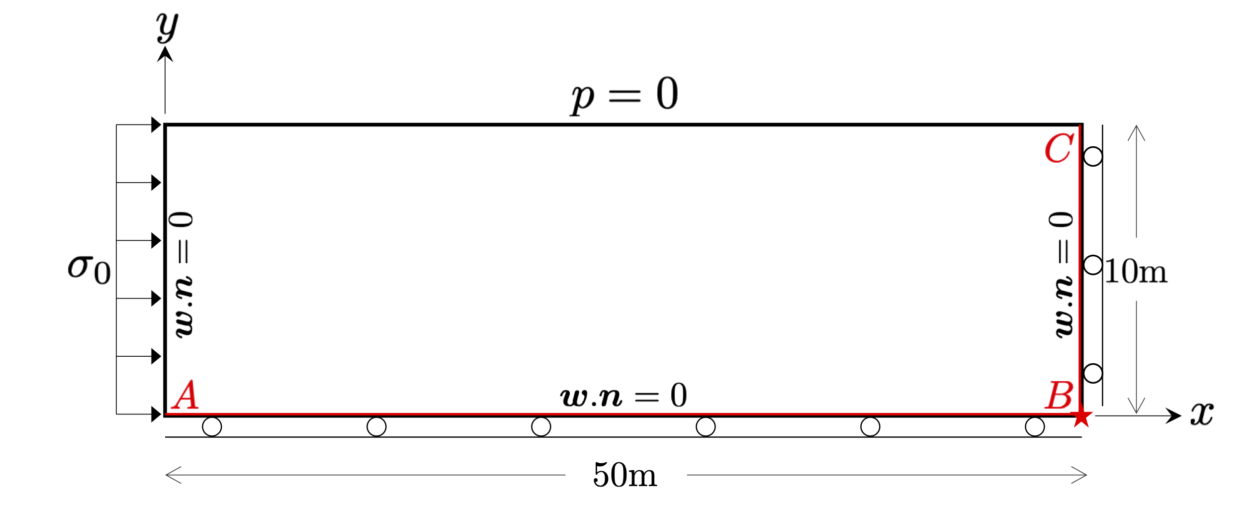
Figure 1: Mandel’s consolidation problem. The left edge is subjected to $\sigma_{0}$ stress while to the top edge is kept traction free. Bottom and right edges are fixed in the normal direction. No-flux boundary condition is imposed on all edges except the top one, where a zero-pressure condition is imposed.

The analytical solution to Mandel’s problem for different value of $D^{*}$ is plotted in Fig. 2. Depending on the choice of $M$ (which changes $D^{*}$), the pressure may exhibit a strong response, almost of the same order as the applied overburden stress, or a weak response to the applied stress. If the coupling is strong (high $D^{*}$), the displacement field also shows a time-varying response. The vertical displacement exceeds the equilibrium displacement due to the change in pore-pressure and gradually returns back to its equilibrium state. These effects are also clear in the $y-log(t)$ plots, along the BC line, shown in Fig. 3.

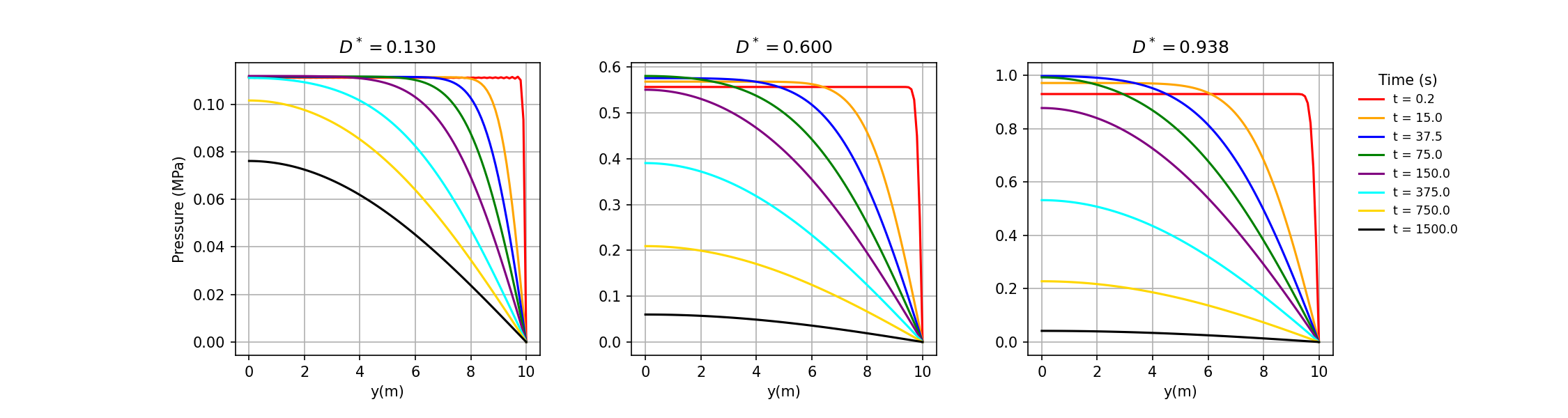
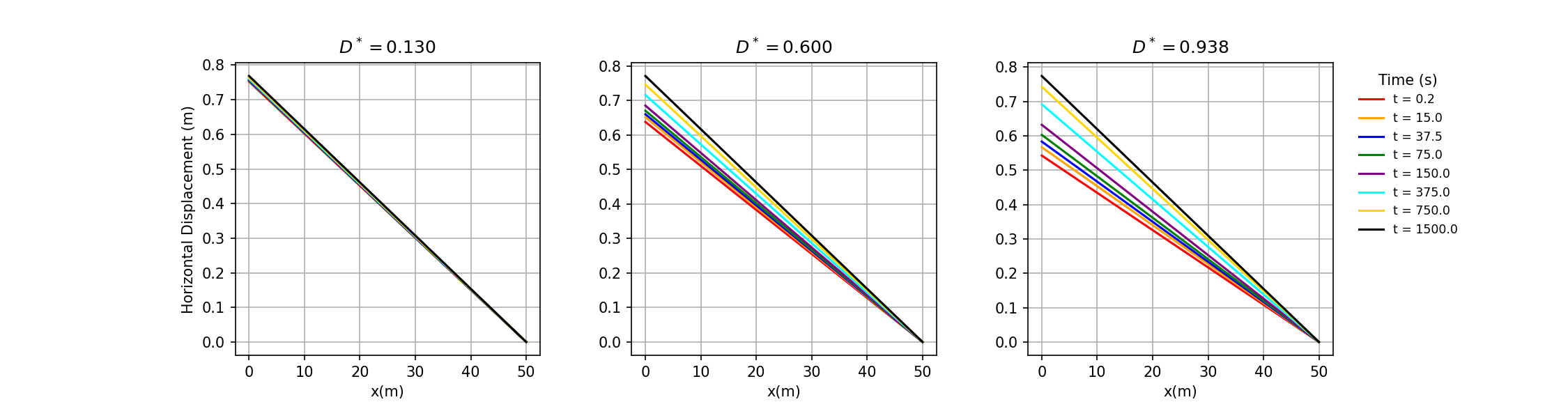
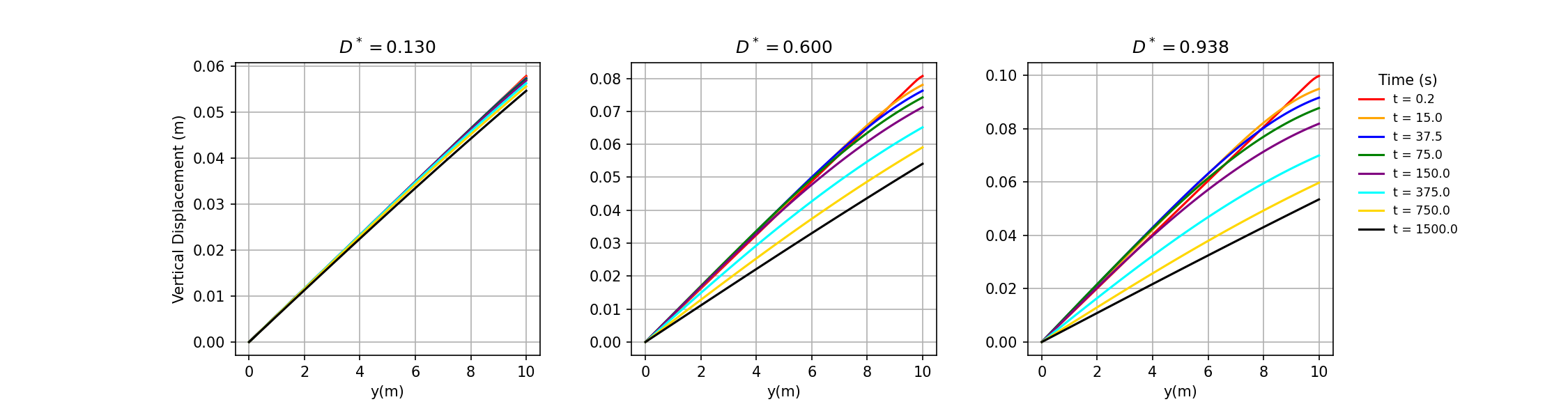
Figure 2: Pore pressure (top), horizontal displacement (middle), and vertical displacement (bottom) for Mandel’s consolidation problem at different times and for different values of $D^{*}$ (left to right, $D^{*}=0.13,~{}0.6,~{}0.938$). Pressure and vertical displacement plots are evaluated along the BC line, while horizontal displacement is evaluated along the AB line, as shown in Fig. 1.

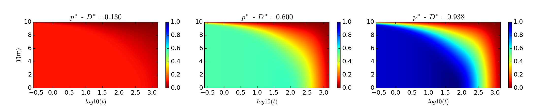
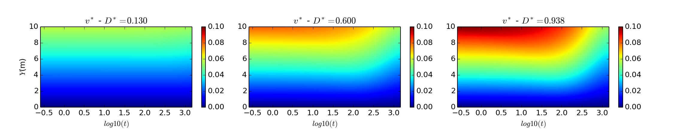
Figure 3: $y-\log t$ contour plots of pressure (top) and vertical displacement (bottom) along BC line (Y-axis) for different values of $D^{*}$ for the Mandel’s consolidation problem.

5.1.1 Training strategies: simultaneous versus stress-split sequential and the role of adaptive weights

We study the convergence of the PINN solution using two different strategies for training the neural network: (1) Simultaneous training using the total loss function (Eq. 60); and (2) Sequential training using the fixed-stress split loss function (Eq. 61). We consider unweighted optimization, i.e., $\lambda_{i}=1$, non-scored adaptive weights based on gradient scaling (referred to as GP) [67] and based on neural tangent kernel (referred to as NTK) [68], and the scored-adaptive-weights GradNorm algorithm [14] discussed above (referred to as GN). We report only the evolution of pore pressure as a function of time along the vertical BC line as shown in Fig. 1. The results of the simultaneous and sequential trainings are summarized in Fig. 4. The most important consideration is if the method can capture the overpressure caused by the Mandel’s setup. We observe that the GradNorm approach with $\alpha=1$ consistently yields the best results, while keep other optimization hyper-parameters unchanged. We additionally find that the fixed-stress sequential approach results in better performance compared to other cases. Therefore the training strategy we adopt for the rest of the paper is based on the use of GradNorm weights with $\alpha=1$ and using the sequential fixed-stress-split strategy.

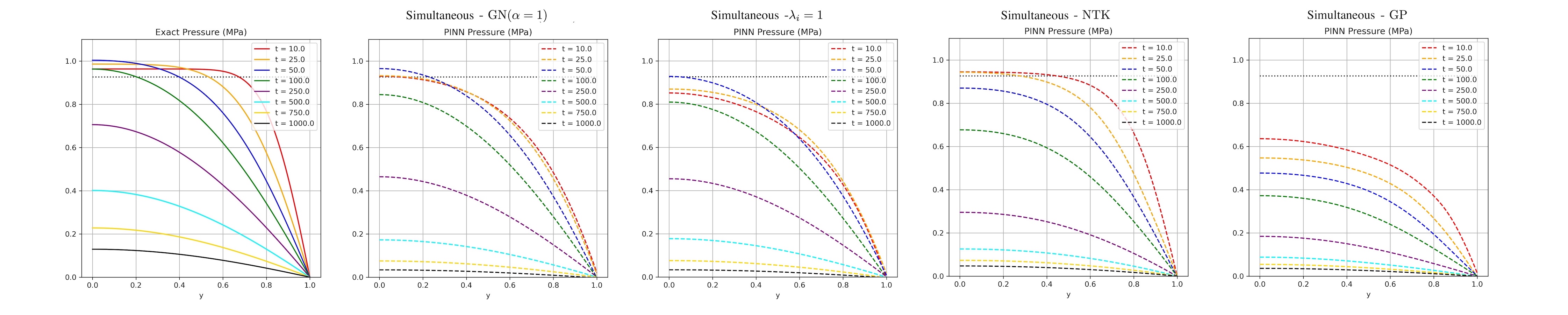
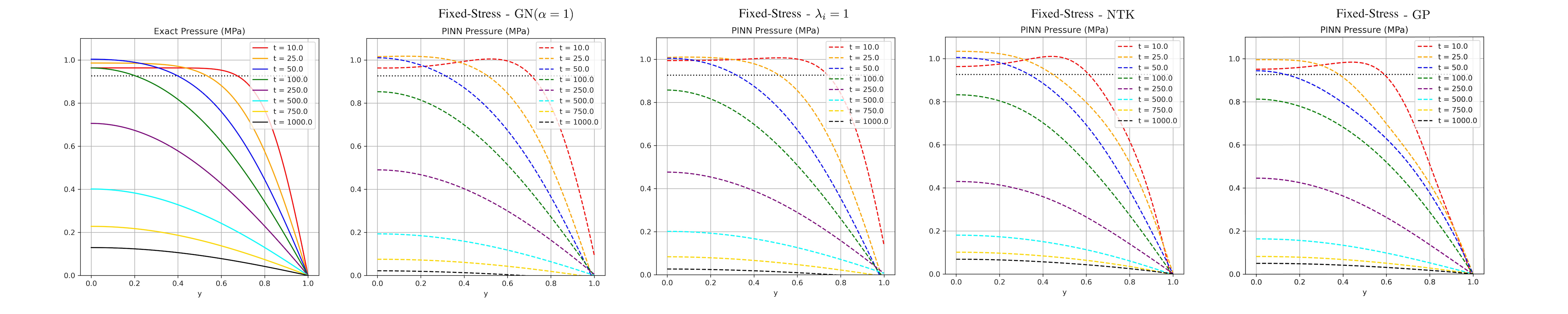
Figure 4: PINN solution for simultaneous (top) and fixed-stress-split sequential (bottom) training, considering adaptive weight schemes including GradNorm ($\alpha=1$), uniform weights with $\lambda_{i}=1$, Neural Tangent Kernel (NTK), and Gradient Pathologies (GP).

5.1.2 Sequential solution: fixed-stress-split vs. fixed-strain-split

Here, we explore the role of the fixed-stress-split and fixed-strain-split strategies for the sequential solution of the coupled system. The two equations describing the flow problem are almost identical, the key difference being the variable passing the information related to the mechanics problem. The results are shown in Fig. 5. The top plots show the stress-split iterations while the bottom plots depict the strain-split iterations. We note that the strain-split strategy diverges while the stress-split formulation converges to the right solution. We note that if we choose $D^{*}$ based on the stability criterion reported by Kim et al. [37], the strain-split strategy also converges to the expected solution. This is a surprising finding of our study because the stability criterion was originally developed for Euler integration of the FEM discretized system while the approximation space of PINNs remains continuous, both in space and time.

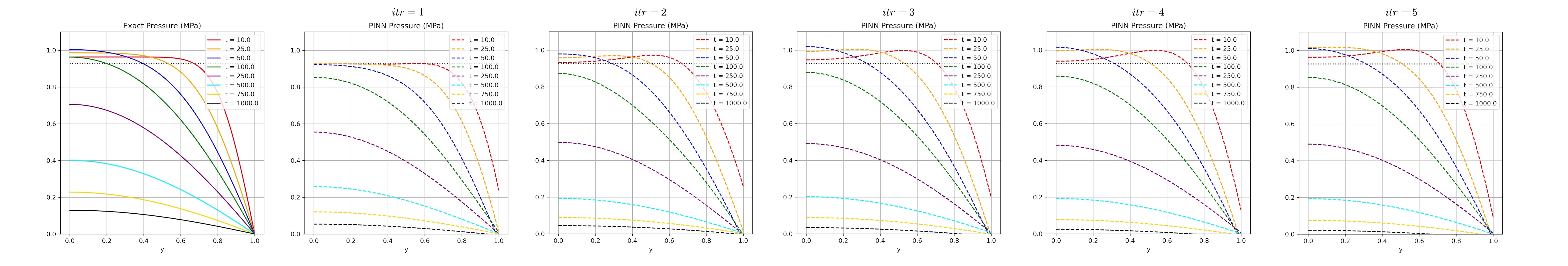
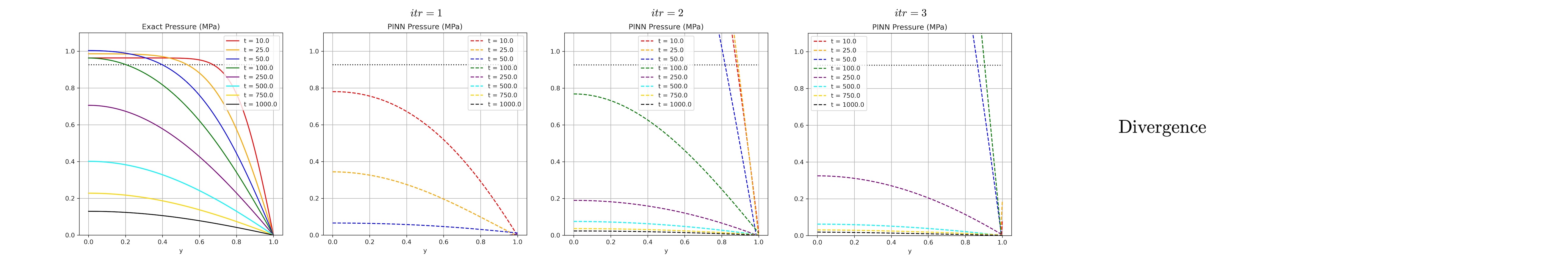
Figure 5: PINN solution for Mandel’s problem using sequential stress-split (top) versus strain-split (bottom) network training. The strain-split approach is not stable for $D^{*}=0.934$ and results in divergence.

5.1.3 PINN’s $D^{*}$-dependence

As it is clear from Eq. 26, $D^{*}$ controls the degree of coupling between flow and mechanics problems, with values ranging in $D^{*}\in(0,1)$. A small value of $D^{*}$ implies no coupling, while a large value implies strong coupling. Here, we assess the quality of the PINN solution as a function of $D^{*}$. The results are plotted in Fig. 6. Not surprisingly, the PINN solutions have highest accuracy for small $D^{*}$. For a fixed set of hyper parameters, the accuracy gradually decreases as $D^{*}$ increases. Note that all of trainings are conducted using the same number of epochs. An equivalent interpretation is that as $D^{*}$ increases, the training requires increasingly more epochs to reach the same accuracy. This observation confirms the challenges associated with PINN solvers for coupled multiphysics problems.

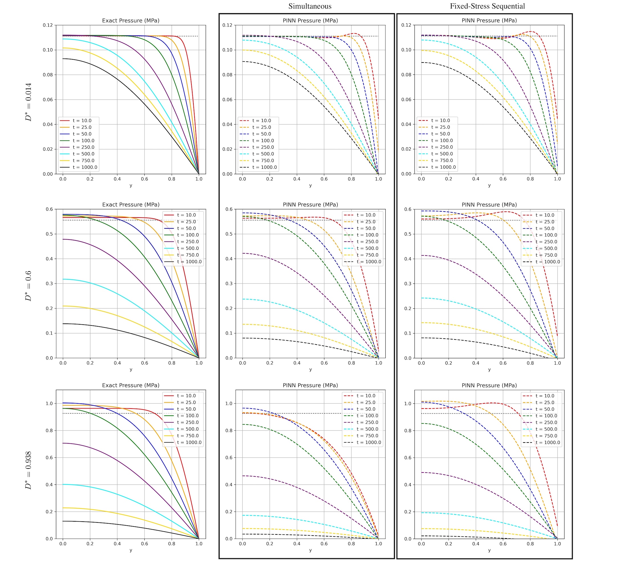
Figure 6: PINN solution for Mandel’s problem and its dependence of $D^{*}$ for simultaneous (middle) and fixed-stress-split sequential (right) solution strategies.

5.1.4 Network size and architecture

It is no surprise that the network size and architecture, as well as the optimizer’s hyper parameters such as learning rate, can also play a critical role in the quality of PINN solutions. For all the examples shown in this manuscript, we have set up neural networks with 4 hidden layers and with 100 neurons in each layer, using the hyperbolic-tangent activation function. The optimizer is Adam, with an initial learning rate of $10^{-3}$, and with an exponential learning decay to $10^{-5}$ at the end of training. We have also experimented with the Fourier feature architecture [69], ResNet architecture, globally and locally adaptive activation functions [28], and SIREN architecture with periodic activation functions [61]. However, we have not seen any significant improvement for solving the coupled flow-mechanics problem studied here.

5.2 Barry-Mercer’s Injection-Production Problem

Practical problems of porous media involve injection and production of fluids. A classical benchmark problem of this type is the Barry-Mercer problem [4], in which a time-dependent fluid injection/production well is considered. In this two-dimensional problem, the gravity term is ignored. The solid and fluid phases are considered incompressible, and Biot’s coefficient is assumed ${b=1}$, which results in ${D^{*}=1.0}$. The initial conditions are zero pressure and displacement in the entire domain. The boundary conditions are depicted in Fig. 7. The analytical solution to this problem is given in the Section A.2.

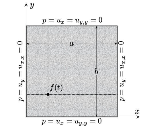
Figure 7: Barry-Mercer’s injection-production problem. All edges are subjected to zero-pressure condition, and they are fixed in their normal direction. A production-injection source term $f(t)$ is applied at $(x_{0},y_{0})$.

In this study, similar to [52], the location of the injection/production point is set equal to ${(x_{0},y_{0})=(0.25,0.25)}$, and the domain length and width are assumed ${a=b=1\text{m}}$. Elastic properties of the solid phase are taken as ${E=4.67~{}\text{MPa}}$ and ${\nu=0.167}$. The permeability and the fluid viscosity are ${k=10^{-10}~{}\text{m}^{2}}$ and ${\mu=10^{-3}~{}\text{Pa.s}}$. The injection/production function $f(t)$ is given by:

$$f(t)={2\beta}{\delta(x-x_{0})\delta(y-y_{0})}{\sin(\beta t)},~{}~{}~{}~{}~{}\text{where}~{}~{}~{}~{}~{}{\beta}=\frac{{E(1-\nu)}k}{(1+\nu)(1-2\nu)ab\mu},$$ (67)

in which ${\delta}$ denotes the Dirac delta function and its Gaussian approximation is used here, i.e., ${\delta(x)}=\frac{1}{\alpha\sqrt{\pi}}{e^{-(x/\alpha)^{2}}}$. In this study, we assume ${\alpha=0.04}$. Note that higher values of $\alpha$ diffuse the injection/production source while smaller values concentrate the source function and make the training increasingly challenging. The temporal domain is taken as ${\hat{t}\in[0,2\pi]}$, where ${\hat{t}}$ is the dimensionless time defined as ${\hat{t}=\beta t}$ [4].

The analytical solution is plotted in Fig. 8. The absolute error plots of the stress-split sequential training are plotted in Fig. 9 and their line plots at 3-points are plotted in Fig. 10. As you can see, compared to the results reported in earlier studies, PINN solution has a great agreement with the expected solution.

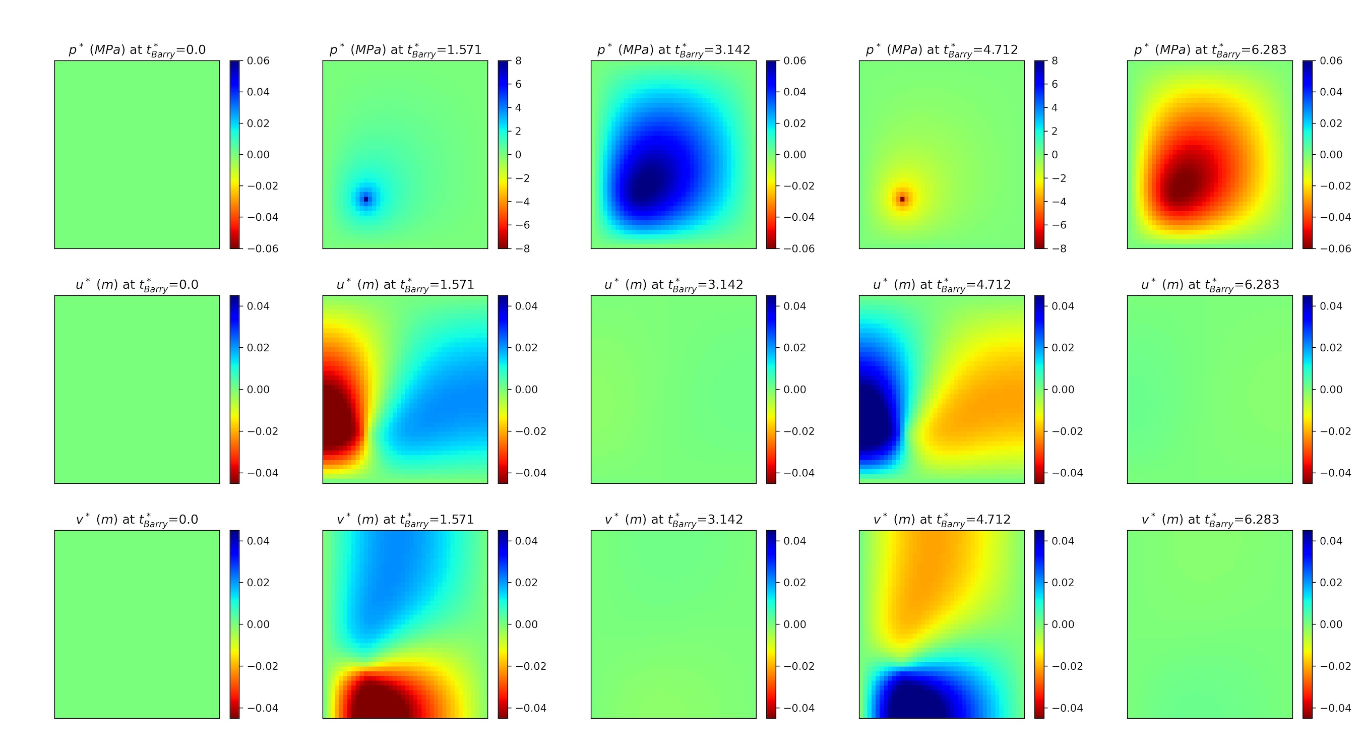
Figure 8: Barry-Mercer’s analytical solution for pore pressure (top), horizontal (middle) and vertical (bottom) displacements, respectively. Each column represents a different time.

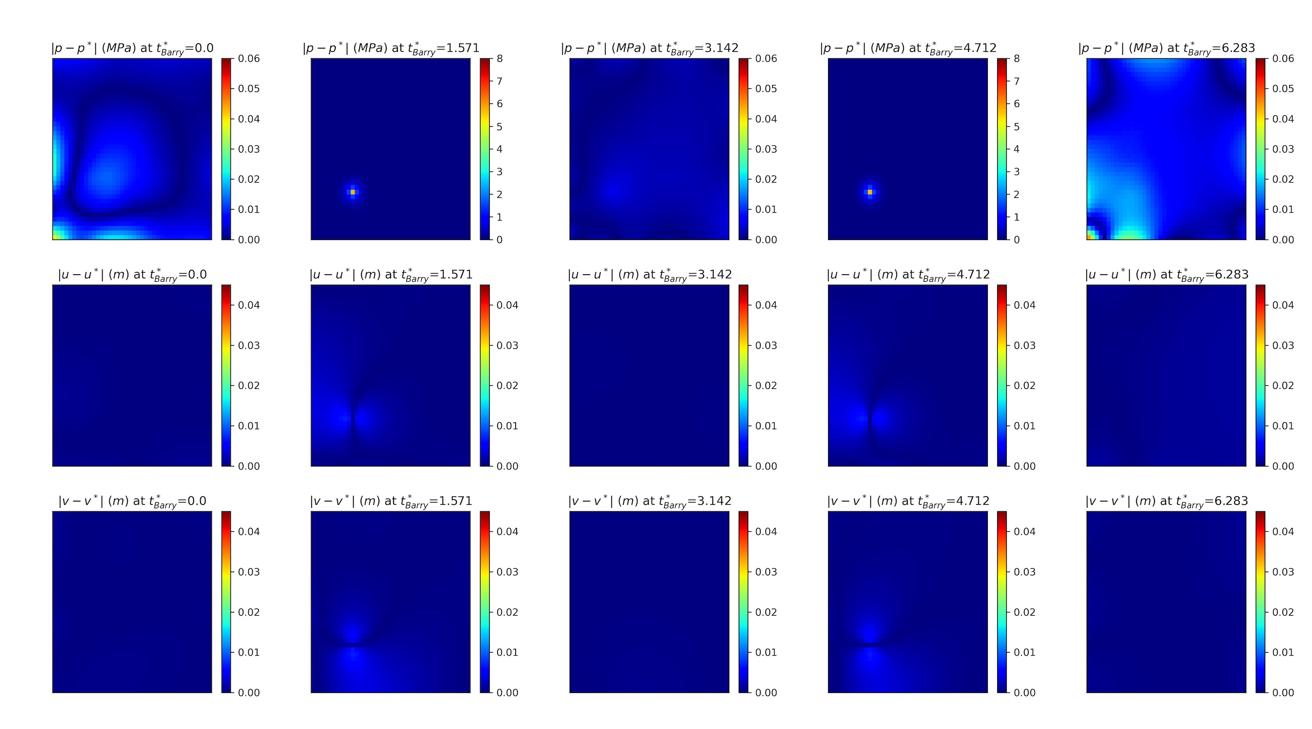
Figure 9: Absolute error plots of Barry-Mercer’s PINN solution for pore pressure (top), horizontal (middle) and vertical (bottom) displacements, respectively, obtained using the fixed-stress-split training strategy. Each column represents a different time. Note that the left two columns represent the solution values at the boundaries.

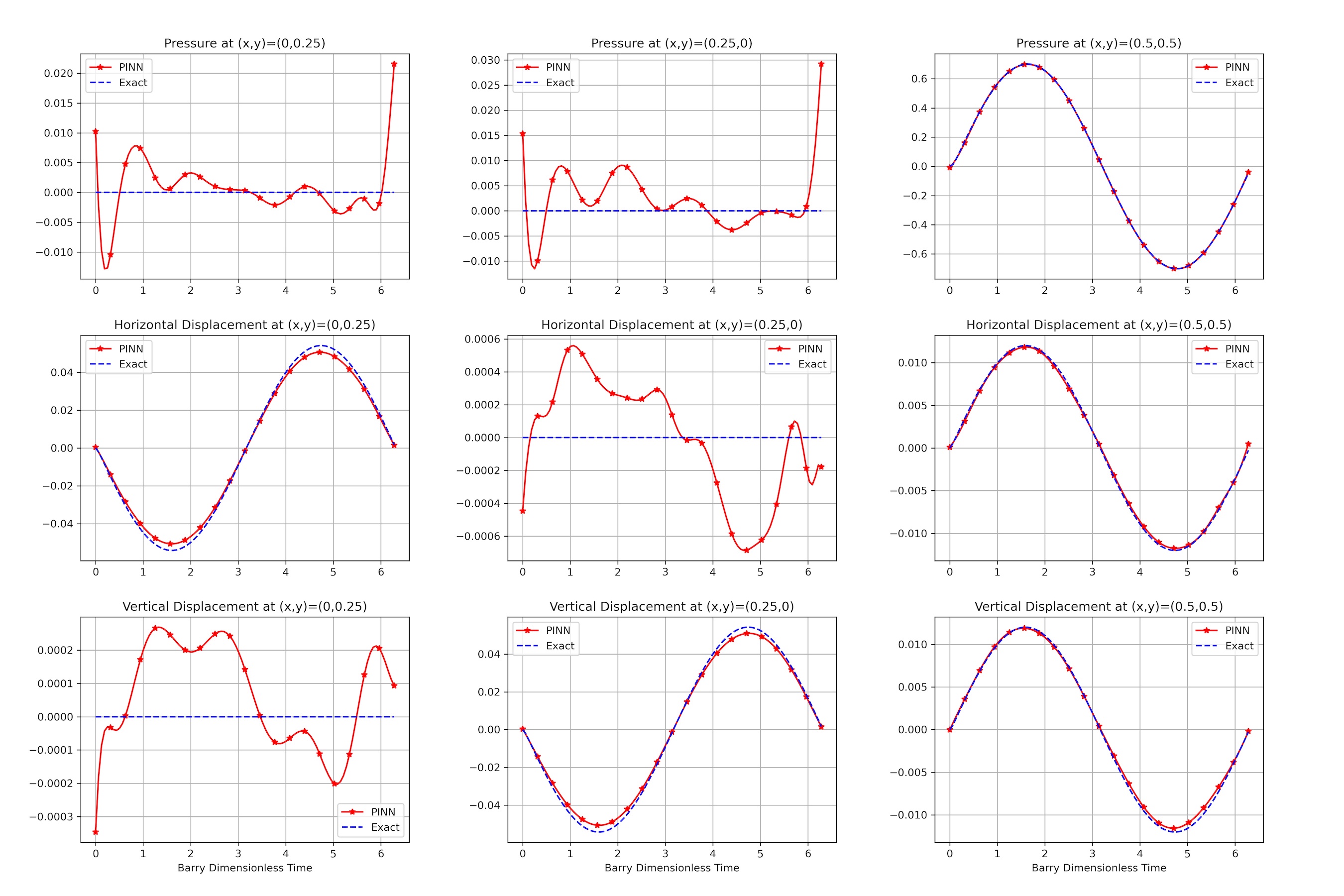
Figure 10: Barry-Mercer’s PINN solution for pore pressure (top), horizontal displacement (middle), and vertical displacement (bottom), respectively, obtained using the fixed-stress-split training strategy. Each column represents a different location around the injection-production well.

5.3 Two-Phase Drainage Problem

As a third example, we consider a synthetic two-phase flow problem, in which water drains from the bottom of a soil column due to gravity. This well-known example was experimentally investigated by Liakopoulos [41] and has been used as a benchmark problem [40]. To impose one-dimensional boundary conditions in the laboratory test, the soil column was placed in an impermeable vessel open at the bottom and top. The column is initially fully saturated with water and in mechanical equilibrium. Then the water inflow is ceased and a no-displacement boundary condition at the bottom together with the free-stress condition at the top surface is imposed. The water pressure at the bottom and gas pressure at both the bottom and top surfaces are set equal to atmospheric pressure. It is assumed that this ${1\text{m}}$ soil column has linear elastic behavior, in which the Young modulus is ${E=1.3\text{MPa}}$, the Poisson ratio is ${\nu=0.4}$, the porosity is ${\phi=0.2975}$, and the Biot coefficient is ${b=1}$. The densities of solid, water, and gas phases are ${\rho_{s}=2400\text{kg}/\text{m}^{3}}$, ${\rho_{w}=1000\text{kg}/\text{m}^{3}}$, and ${\rho_{g}=1.2\text{kg}/\text{m}^{3}}$, respectively. The fluid compressibilities are ${c_{w}={{5}\times 10^{-10}}\text{Pa}^{-1}}$, ${c_{g}={10^{-5}}\text{Pa}^{-1}}$, with the solid bulk modulus ${K_{s}={10^{12}}\text{Pa}}$. In this numerical test, the intrinsic permeability is ${k={4.5}\times{10^{-13}}\text{m}^{2}}$, the gravitational acceleration is ${g={9.806}\text{m}/\text{s}^{2}}$, and the atmospheric pressure is zero. Furthermore, although the saturation relation, as well as relative permeability function for the water phase, are obtained from experimental expressions, the relative permeability of the gas phase is calculated by Brooks-Corey [9] model as follows

$${p_{c}} =2.57\rho_{w}g(1-S_{w})^{\frac{1}{2.4279}},$$

$${k_{rw}} ={1-2.2{(1-S_{w})}},$$

$${k_{rg}} =\text{max}{[(1-S_{e})^{2}(1-S_{e}^{{(2+\lambda)}/{\lambda}}),0.0001]},$$

$${{S_{e}}} ={(S_{w}-S_{rw})}/{(1-S_{rw})}.$$

where ${\lambda=3}$, denotes the pore size distribution, ${S_{e}}$ is the effective saturation, and ${S_{rw}=0.2}$ is the connate water saturation. In addition, the fluid viscosities are ${\mu_{w}={10^{-3}}\text{Pa.s}}$, ${\mu_{g}={1.8}\times{10^{-5}}\text{Pa.s}}$. The results are plotted in Fig. 11, which are in agreement with the expected results.

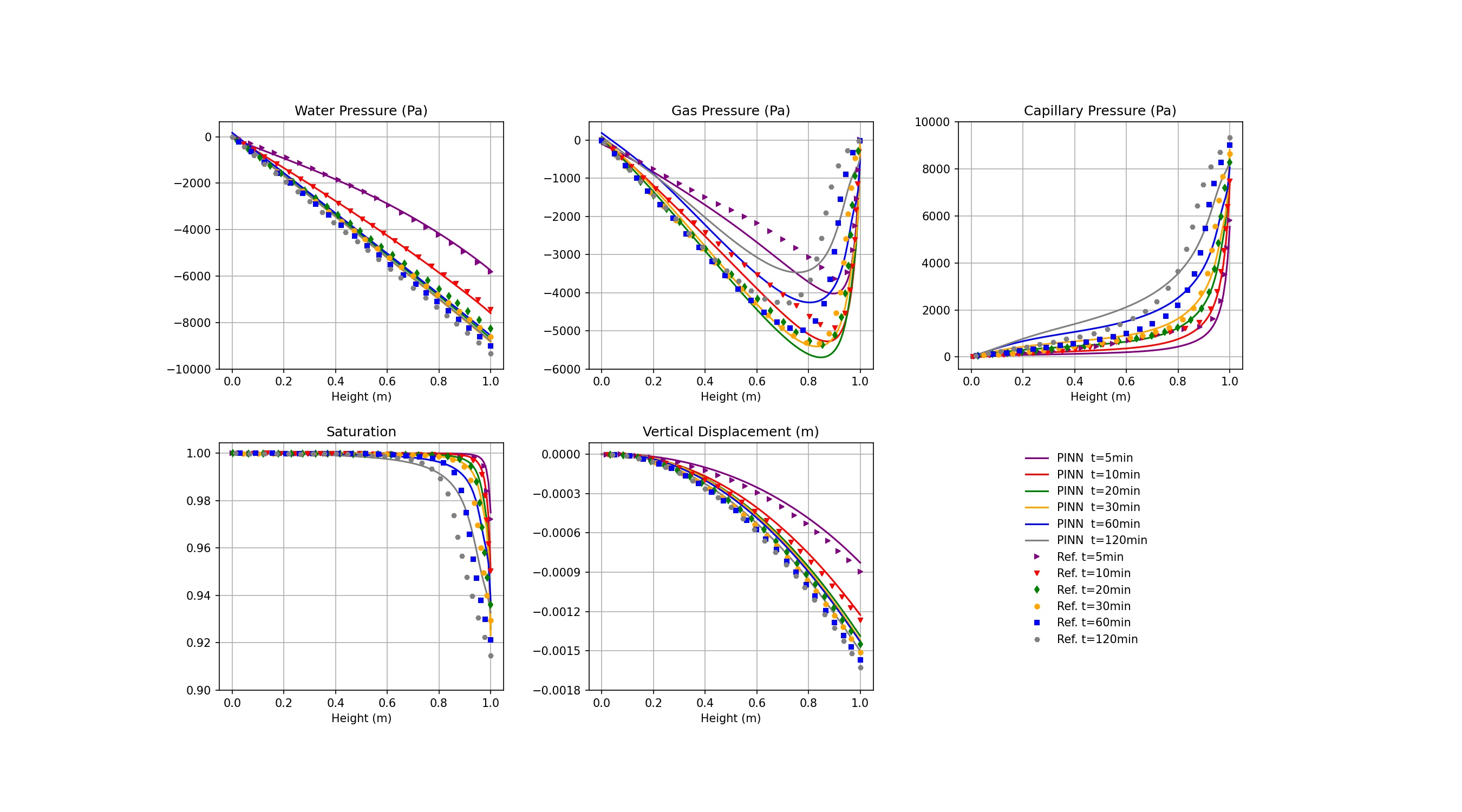
Figure 11: The PINN solution for the two-phase soil column water drainage problem, at different times. The reference solution is reproduced form the results reported by Lewis et al. [40].

6 Discussions and Concluding Remarks

We study an application of Physics-Informed Neural Networks (PINNs) for the forward solution of coupled fully- and partially-saturated porous media. Our study is the first to consider fully coupled relations of porous media under single-phase and two-phase flow conditions. We report a dimensionless form of these relations that results in a stable and convergent behavior of the optimizer. One of the key contributions from this work is proposing a novel sequential training of the neural network. In the current application to poromechanics problems, it takes the form of a fixed-stress split of the loss function. This training strategy results in enhanced convergence and robustness of the PINN formulation.

While our results show good agreement with expected results, we still find that training PINNs is very slow and control over its accuracy is challenging. As reported by others, we associate the training challenge to the multi-objective optimization problem and the use of a first-order optimization method. Considering the challenges faced and resolved in this study for the forward problem, a next step is to apply PINNs for inverse problems of coupled multiphase flow and poroelasticity.

Appendix A Analytical solutions

For completeness, we report the analytical solutions that exist for Mandel’s problem as well as for Barry-Mercer’s problem. A summary of these solutions are also discussed in [12, 52].

A.1 Mandel’s analytical solution

The analytical solution to the Mandel’s consolidation problem is expressed as

$${p(x,y,t)} =\frac{2|\sigma_{0}|B(1+\nu_{u})}{3}\left(\sum_{i=1}^{\infty}\frac{\sin\alpha_{i}}{\alpha_{i}-\sin\alpha_{i}\cos\alpha_{i}}~{}({\cos(\frac{\alpha_{i}y}{L_{y}})-{\cos\alpha_{i}})}~{}\exp[\frac{-\alpha_{i}^{2}c_{f}t}{L_{y}^{2}}]\right),$$

$${v(x,y,t)} =\frac{\sigma_{0}y}{G}\left(\frac{\nu}{2}-{\nu_{u}}\sum_{i=1}^{\infty}\frac{\sin\alpha_{i}\cos\alpha_{i}}{\alpha_{i}-\sin\alpha_{i}\cos\alpha_{i}}~{}\exp[\frac{-\alpha_{i}^{2}c_{f}t}{L_{y}^{2}}]\right)$$

$$+\frac{\sigma_{0}L_{y}}{G}\left(\sum_{i=1}^{\infty}\frac{\cos\alpha_{i}}{\alpha_{i}-\sin\alpha_{i}\cos\alpha_{i}}~{}{\sin(\frac{\alpha_{i}y}{L_{y}})}~{}\exp[\frac{-\alpha_{i}^{2}c_{f}t}{L_{y}^{2}}]\right),$$

$${u(x,y,t)} =\frac{\sigma_{0}(L_{x}-x)}{G}\left(\frac{-(1-\nu)}{2}+(1-\nu_{u})\sum_{i=1}^{\infty}\frac{\sin\alpha_{i}\cos\alpha_{i}}{\alpha_{i}-\sin\alpha_{i}\cos\alpha_{i}}~{}\exp[\frac{-\alpha_{i}^{2}c_{f}t}{L_{y}^{2}}]\right).$$

where the parameters are

$${B} =\frac{bM}{K_{dr}+{b^{2}}{M}},$$

$${\nu_{u}} =\frac{3\nu+bB(1-2\nu)}{3-bB(1-2\nu)},$$

$${c_{f}} =\frac{k}{\mu(1/M+{b^{2}}/{K_{dr}})},$$

$${G} =\frac{E}{2(1+\nu)}$$

It must be noted that ${\sigma_{0}}$ is negative for compression loading and positive for tension loading, and ${\alpha_{i}}$ are the roots of the equation:

$${\tan\alpha_{i}}=\frac{1-\nu}{\nu_{u}-\nu}{\alpha_{i}}.$$

A.2 Barry-Mercer’s problem

Assuming the parameters

$${\lambda_{n}} ={n\pi},$$

$${\lambda_{q}} ={q\pi},$$

$${\lambda_{nq}} ={\lambda_{n}^{2}}+{\lambda_{q}^{2}},$$

$${\beta} =\frac{{E(1-\nu)}k}{(1+\nu)(1-2\nu)ab\mu},$$

and with an injection function of the form

$${Q}={2\beta}{\delta(x-x_{0})\delta(y-y_{0})}{\sin(\beta t)}$$

with $(x_{0},y_{0})$ as source location. The time domain is considered as ${\hat{t}\in[0,2\pi]}$, where ${\hat{t}=\beta t}$. Definition of the pressure, horizontal and vertical displacement in the transformed coordinate :

$${\hat{p}(n,q,t)} =\frac{-2\sin(\lambda_{n}x_{0})\sin(\lambda_{q}y_{0})}{\lambda_{nq}^{2}+1}(\lambda_{nq}\sin(\beta t)-\cos(\beta t)+{e^{-\lambda_{nq}\beta t}}),$$

$${\hat{u}(n,q,t)} =\frac{\lambda_{n}}{\lambda_{n}q}{\hat{p}(n,q,t)},$$

$${\hat{v}(n,q,t)} =\frac{\lambda_{q}}{\lambda_{n}q}{\hat{p}(n,q,t)},$$

The real pressure, horizontal and vertical displacement in the real coordinates can be defined as:

$${p(x,y,t)} =\frac{-4E(1-\nu)}{(1+\nu)(1-2\nu)}{\sum_{n=1}^{\infty}}~{}{\sum_{q=1}^{\infty}{\hat{p}(n,q,t)}{\sin(\lambda_{n}x)}{\sin(\lambda_{q}y)}},$$

$${u(x,y,t)} ={4}{\sum_{n=1}^{\infty}}~{}{\sum_{q=1}^{\infty}{\hat{u}(n,q,t)}{\cos(\lambda_{n}x)}{\sin(\lambda_{q}y)}},$$

$${v(x,y,t)} ={4}{\sum_{n=1}^{\infty}}~{}{\sum_{q=1}^{\infty}{\hat{v}(n,q,t)}{\sin(\lambda_{n}x)}{\cos(\lambda_{q}y)}}.$$

References

- Almajid and Abu-Alsaud [2022] Muhammad M Almajid and Moataz O Abu-Alsaud. Prediction of porous media fluid flow using physics informed neural networks. Journal of Petroleum Science and Engineering, 208:109205, 2022.
- Armero and Simo [1992] F Armero and JC Simo. A new unconditionally stable fractional step method for non-linear coupled thermomechanical problems. International Journal for numerical methods in Engineering, 35(4):737–766, 1992.
- Armero [1999] Francisco Armero. Formulation and finite element implementation of a multiplicative model of coupled poro-plasticity at finite strains under fully saturated conditions. Computer methods in applied mechanics and engineering, 171(3-4):205–241, 1999.
- Barry and Mercer [1999] S. I. Barry and G. N. Mercer. Exact Solutions for Two-Dimensional Time-Dependent Flow and Deformation Within a Poroelastic Medium. Journal of Applied Mechanics, 66(2):536–540, 1999.
- Bekele [2020] Yared W Bekele. Physics-informed deep learning for flow and deformation in poroelastic media. arXiv preprint arXiv:2010.15426, 2020.
- Bekele [2021] Yared W Bekele. Physics-informed deep learning for one-dimensional consolidation. Journal of Rock Mechanics and Geotechnical Engineering, 13(2):420–430, 2021.
- bin Waheed et al. [2021] Umair bin Waheed, Ehsan Haghighat, Tariq Alkhalifah, Chao Song, and Qi Hao. PINNeik: Eikonal solution using physics-informed neural networks. Computers & Geosciences, 155:104833, 2021.
- Biot [1941] Maurice A Biot. General theory of three-dimensional consolidation. Journal of applied physics, 12(2):155–164, 1941.
- Brooks and Corey [1966] Royal Harvard Brooks and Arthur T Corey. Properties of porous media affecting fluid flow. Journal of the Irrigation and Drainage Division, 92(2):61–88, 1966.
- Cai et al. [2021a] Shengze Cai, Zhiping Mao, Zhicheng Wang, Minglang Yin, and George Em Karniadakis. Physics-informed neural networks (PINNs) for fluid mechanics: A review. arXiv preprint arXiv:2105.09506, 2021a.
- Cai et al. [2021b] Shengze Cai, Zhicheng Wang, Sifan Wang, Paris Perdikaris, and George Em Karniadakis. Physics-informed neural networks for heat transfer problems. Journal of Heat Transfer, 143(6):060801, 2021b.
- Castelletto et al. [2015] Nicola Castelletto, Joshua A White, and HA Tchelepi. Accuracy and convergence properties of the fixed-stress iterative solution of two-way coupled poromechanics. International Journal for Numerical and Analytical Methods in Geomechanics, 39(14):1593–1618, 2015.
- Chen et al. [2020] Yuyao Chen, Lu Lu, George Em Karniadakis, and Luca Dal Negro. Physics-informed neural networks for inverse problems in nano-optics and metamaterials. Optics express, 28(8):11618–11633, 2020.
- Chen et al. [2018] Zhao Chen, Vijay Badrinarayanan, Chen-Yu Lee, and Andrew Rabinovich. Gradnorm: Gradient normalization for adaptive loss balancing in deep multitask networks. In International Conference on Machine Learning, pages 794–803. PMLR, 2018.
- Coussy [2004] Olivier Coussy. Poromechanics. John Wiley & Sons, 2004.
- Fang and Zhan [2019] Zhiwei Fang and Justin Zhan. Deep physical informed neural networks for metamaterial design. IEEE Access, 8:24506–24513, 2019.
- Fraces et al. [2020] Cedric G Fraces, Adrien Papaioannou, and Hamdi Tchelepi. Physics informed deep learning for transport in porous media. Buckley Leverett problem. arXiv preprint arXiv:2001.05172, 2020.
- Fredrich et al. [2000] Joanne T Fredrich, JG Arguello, GL Deitrick, and Eric P de Rouffignac. Geomechanical modeling of reservoir compaction, surface subsidence, and casing damage at the belridge diatomite field. SPE Reservoir Evaluation & Engineering, 3(04):348–359, 2000.
- Fuks and Tchelepi [2020] Olga Fuks and Hamdi A Tchelepi. Limitations of physics informed machine learning for nonlinear two-phase transport in porous media. Journal of Machine Learning for Modeling and Computing, 1(1):19–37, 2020.
- Garipov et al. [2018] Timur T Garipov, Pavel Tomin, Ruslan Rin, Denis V Voskov, and Hamdi A Tchelepi. Unified thermo-compositional-mechanical framework for reservoir simulation. Computational Geosciences, 22(4):1039–1057, 2018.
- Guo and Haghighat [2020] Mengwu Guo and Ehsan Haghighat. An energy-based error bound of physics-informed neural network solutions in elasticity. arXiv preprint arXiv:2010.09088, 2020.
- Haghighat and Juanes [2021] Ehsan Haghighat and Ruben Juanes. SciANN: A Keras/TensorFlow wrapper for scientific computations and physics-informed deep learning using artificial neural networks. Computer Methods in Applied Mechanics and Engineering, 373:113552, 2021.
- Haghighat et al. [2021a] Ehsan Haghighat, Ali Can Bekar, Erdogan Madenci, and Ruben Juanes. A nonlocal physics-informed deep learning framework using the peridynamic differential operator. Computer Methods in Applied Mechanics and Engineering, 385:114012, 2021a.
- Haghighat et al. [2021b] Ehsan Haghighat, Maziar Raissi, Adrian Moure, Hector Gomez, and Ruben Juanes. A physics-informed deep learning framework for inversion and surrogate modeling in solid mechanics. Computer Methods in Applied Mechanics and Engineering, 379:113741, 2021b.
- Hennigh et al. [2021] Oliver Hennigh, Susheela Narasimhan, Mohammad Amin Nabian, Akshay Subramaniam, Kaustubh Tangsali, Zhiwei Fang, Max Rietmann, Wonmin Byeon, and Sanjay Choudhry. NVIDIA SimNet™: An AI-accelerated multi-physics simulation framework. In International Conference on Computational Science, pages 447–461. Springer, 2021.
- Hughes [2012] Thomas JR Hughes. The finite element method: linear static and dynamic finite element analysis. Courier Corporation, 2012.
- Jagtap and Karniadakis [2020] Ameya D Jagtap and George Em Karniadakis. Extended physics-informed neural networks (xPINNs): A generalized space-time domain decomposition based deep learning framework for nonlinear partial differential equations. Communications in Computational Physics, 28(5):2002–2041, 2020.
- Jagtap et al. [2020a] Ameya D Jagtap, Kenji Kawaguchi, and George Em Karniadakis. Locally adaptive activation functions with slope recovery for deep and physics-informed neural networks. Proceedings of the Royal Society A, 476(2239):20200334, 2020a.
- Jagtap et al. [2020b] Ameya D Jagtap, Ehsan Kharazmi, and George Em Karniadakis. Conservative physics-informed neural networks on discrete domains for conservation laws: Applications to forward and inverse problems. Computer Methods in Applied Mechanics and Engineering, 365:113028, 2020b.
- Jha and Juanes [2007] Birendra Jha and Ruben Juanes. A locally conservative finite element framework for the simulation of coupled flow and reservoir geomechanics. Acta Geotechnica, 2(3):139–153, 2007.
- Jha and Juanes [2014] Birendra Jha and Ruben Juanes. Coupled multiphase flow and poromechanics: A computational model of pore pressure effects on fault slip and earthquake triggering. Water Resources Research, 50(5):3776–3808, 2014.
- Ji et al. [2020] Weiqi Ji, Weilun Qiu, Zhiyu Shi, Shaowu Pan, and Sili Deng. Stiff-pinn: Physics-informed neural network for stiff chemical kinetics. arXiv preprint arXiv:2011.04520, 2020.
- Jin et al. [2021] Xiaowei Jin, Shengze Cai, Hui Li, and George Em Karniadakis. NSFnets (Navier-Stokes flow nets): Physics-informed neural networks for the incompressible Navier-Stokes equations. Journal of Computational Physics, 426:109951, 2021.
- Kadeethum et al. [2020] Teeratorn Kadeethum, Thomas M Jørgensen, and Hamidreza M Nick. Physics-informed neural networks for solving nonlinear diffusivity and biot’s equations. PLoS One, 15(5):e0232683, 2020.
- Karniadakis et al. [2021] George Em Karniadakis, Ioannis G Kevrekidis, Lu Lu, Paris Perdikaris, Sifan Wang, and Liu Yang. Physics-informed machine learning. Nature Reviews Physics, 3(6):422–440, 2021.
- Khoei and Mohammadnejad [2011] AR Khoei and T Mohammadnejad. Numerical modeling of multiphase fluid flow in deforming porous media: A comparison between two-and three-phase models for seismic analysis of earth and rockfill dams. Computers and Geotechnics, 38(2):142–166, 2011.
- Kim et al. [2011] Jihoon Kim, Hamdi A Tchelepi, and Ruben Juanes. Stability and convergence of sequential methods for coupled flow and geomechanics: Fixed-stress and fixed-strain splits. Computer Methods in Applied Mechanics and Engineering, 200(13-16):1591–1606, 2011.
- Kim et al. [2013] Jihoon Kim, Hamdi A Tchelepi, and Ruben Juanes. Rigorous coupling of geomechanics and multiphase flow with strong capillarity. SPE journal, 18(06):1123–1139, 2013.
- Kingma and Ba [2014] Diederik P Kingma and Jimmy Ba. Adam: A method for stochastic optimization. arXiv preprint arXiv:1412.6980, 2014.
- Lewis et al. [1998] Roland Wynne Lewis, Roland W Lewis, and BA Schrefler. The finite element method in the static and dynamic deformation and consolidation of porous media. John Wiley & Sons, 1998.
- Liakopoulos [1964] Aristides C Liakopoulos. Transient flow through unsaturated porous media. University of California, Berkeley, 1964.
- Liu and Nocedal [1989] Dong C Liu and Jorge Nocedal. On the limited memory bfgs method for large scale optimization. Mathematical programming, 45(1):503–528, 1989.
- Liu et al. [2021] Sen Liu, Branden B Kappes, Behnam Amin-ahmadi, Othmane Benafan, Xiaoli Zhang, and Aaron P Stebner. Physics-informed machine learning for composition–process–property design: Shape memory alloy demonstration. Applied Materials Today, 22:100898, 2021.
- Lu et al. [2021] Lu Lu, Xuhui Meng, Zhiping Mao, and George Em Karniadakis. DeepXDE: A deep learning library for solving differential equations. SIAM Review, 63(1):208–228, 2021.
- Madenci et al. [2016] Erdogan Madenci, Atila Barut, and Michael Futch. Peridynamic differential operator and its applications. Computer Methods in Applied Mechanics and Engineering, 304:408–451, 2016.
- Mao et al. [2020] Zhiping Mao, Ameya D Jagtap, and George Em Karniadakis. Physics-informed neural networks for high-speed flows. Computer Methods in Applied Mechanics and Engineering, 360:112789, 2020.
- Nabian et al. [2021] Mohammad Amin Nabian, Rini Jasmine Gladstone, and Hadi Meidani. Efficient training of physics-informed neural networks via importance sampling. Computer-Aided Civil and Infrastructure Engineering, 2021.
- Niaki et al. [2021] Sina Amini Niaki, Ehsan Haghighat, Trevor Campbell, Anoush Poursartip, and Reza Vaziri. Physics-informed neural network for modelling the thermochemical curing process of composite-tool systems during manufacture. Computer Methods in Applied Mechanics and Engineering, 384:113959, 2021.
- Noakoasteen et al. [2020] Oameed Noakoasteen, Shu Wang, Zhen Peng, and Christos Christodoulou. Physics-informed deep neural networks for transient electromagnetic analysis. IEEE Open Journal of Antennas and Propagation, 1:404–412, 2020.
- Nocedal and Wright [2006] Jorge Nocedal and Stephen Wright. Numerical optimization. Springer Science & Business Media, 2006.
- Park [1983] KC Park. Stabilization of partitioned solution procedure for pore fluid-soil interaction analysis. International Journal for Numerical Methods in Engineering, 19(11):1669–1673, 1983.
- Phillips [2005] Phillip Joseph Phillips. Finite element methods in linear poroelasticity: Theoretical and computational results. The University of Texas at Austin, 2005.
- Pilania et al. [2018] Ghanshyam Pilania, Kenneth James McClellan, Christopher Richard Stanek, and Blas P Uberuaga. Physics-informed machine learning for inorganic scintillator discovery. The Journal of chemical physics, 148(24):241729, 2018.
- Raissi et al. [2019] Maziar Raissi, Paris Perdikaris, and George E Karniadakis. Physics-informed neural networks: A deep learning framework for solving forward and inverse problems involving nonlinear partial differential equations. Journal of Computational Physics, 378:686–707, 2019.
- Rao et al. [2020] Chengping Rao, Hao Sun, and Yang Liu. Physics-informed deep learning for incompressible laminar flows. Theoretical and Applied Mechanics Letters, 10(3):207–212, 2020.
- Rao et al. [2021] Chengping Rao, Hao Sun, and Yang Liu. Physics-informed deep learning for computational elastodynamics without labeled data. Journal of Engineering Mechanics, 147(8):04021043, 2021.
- Reyes et al. [2021] Brandon Reyes, Amanda A Howard, Paris Perdikaris, and Alexandre M Tartakovsky. Learning unknown physics of non-newtonian fluids. Physical Review Fluids, 6(7):073301, 2021.
- Schrefler [2004] BA Schrefler. Multiphase flow in deforming porous material. International Journal for Numerical Methods in Engineering, 60(1):27–50, 2004.
- Settari and Mourits [1998] Antonin Settari and FM Mourits. A coupled reservoir and geomechanical simulation system. SPE Journal, 3(03):219–226, 1998.
- Shokouhi et al. [2021] Parisa Shokouhi, Vikas Kumar, Sumedha Prathipati, Seyyed A Hosseini, Clyde Lee Giles, and Daniel Kifer. Physics-informed deep learning for prediction of CO2 storage site response. Journal of Contaminant Hydrology, page 103835, 2021.
- Sitzmann et al. [2020] Vincent Sitzmann, Julien Martel, Alexander Bergman, David Lindell, and Gordon Wetzstein. Implicit neural representations with periodic activation functions. Advances in Neural Information Processing Systems, 33, 2020.
- Song and Alkhalifah [2021] Chao Song and Tariq Alkhalifah. Wavefield reconstruction inversion via physics-informed neural networks. arXiv preprint arXiv:2104.06897, 2021.
- Song et al. [2021] Chao Song, Tariq Alkhalifah, and Umair Bin Waheed. Solving the frequency-domain acoustic VTI wave equation using physics-informed neural networks. Geophysical Journal International, 225(2):846–859, 2021.
- Tartakovsky et al. [2020] Alexandre M Tartakovsky, C Ortiz Marrero, Paris Perdikaris, Guzel D Tartakovsky, and David Barajas-Solano. Physics-informed deep neural networks for learning parameters and constitutive relationships in subsurface flow problems. Water Resources Research, 56(5):e2019WR026731, 2020.
- Thomas et al. [2003] LK Thomas, LY Chin, RG Pierson, and JE Sylte. Coupled geomechanics and reservoir simulation. SPE Journal, 8(04):350–358, 2003.
- Waheed et al. [2021] Umair bin Waheed, Tariq Alkhalifah, Ehsan Haghighat, and Chao Song. A holistic approach to computing first-arrival traveltimes using neural networks. arXiv preprint arXiv:2101.11840, 2021.
- Wang et al. [2020a] Sifan Wang, Yujun Teng, and Paris Perdikaris. Understanding and mitigating gradient pathologies in physics-informed neural networks. arXiv preprint arXiv:2001.04536, 2020a.
- Wang et al. [2020b] Sifan Wang, Xinling Yu, and Paris Perdikaris. When and why PINNs fail to train: A neural tangent kernel perspective. arXiv preprint arXiv:2007.14527, 2020b.
- Wang et al. [2021] Sifan Wang, Hanwen Wang, and Paris Perdikaris. On the eigenvector bias of fourier feature networks: From regression to solving multi-scale PDEs with physics-informed neural networks. Computer Methods in Applied Mechanics and Engineering, 384:113938, 2021.
- White and Borja [2008] Joshua A White and Ronaldo I Borja. Stabilized low-order finite elements for coupled solid-deformation/fluid-diffusion and their application to fault zone transients. Computer Methods in Applied Mechanics and Engineering, 197(49-50):4353–4366, 2008.
- Wight and Zhao [2020] Colby L Wight and Jia Zhao. Solving Allen-Cahn and Cahn-Hilliard equations using the adaptive physics informed neural networks. arXiv preprint arXiv:2007.04542, 2020.
- Wu et al. [2018] Jin-Long Wu, Heng Xiao, and Eric Paterson. Physics-informed machine learning approach for augmenting turbulence models: A comprehensive framework. Physical Review Fluids, 3(7):074602, 2018.
- Zienkiewicz et al. [1988] OC Zienkiewicz, DK Paul, and AHC Chan. Unconditionally stable staggered solution procedure for soil-pore fluid interaction problems. International Journal for Numerical Methods in Engineering, 26(5):1039–1055, 1988.
- Zienkiewicz et al. [1999] O.C. Zienkiewicz, A.H.C. Chan, M. Pastor, B.A. Schrefler, and T. Shiomi. Computational Geomechanics with Special Reference to Earthquake Engineering. Wiley, 1999. ISBN 9780471982852.
- Zienkiewicz et al. [1977] Olgierd Cecil Zienkiewicz, Robert Leroy Taylor, Perumal Nithiarasu, and JZ Zhu. The finite element method, volume 3. McGraw-hill London, 1977.
- Zobeiry and Humfeld [2021] Navid Zobeiry and Keith D Humfeld. A physics-informed machine learning approach for solving heat transfer equation in advanced manufacturing and engineering applications. Engineering Applications of Artificial Intelligence, 101:104232, 2021.
- Zubov et al. [2021] Kirill Zubov, Zoe McCarthy, Yingbo Ma, Francesco Calisto, Valerio Pagliarino, Simone Azeglio, Luca Bottero, Emmanuel Luján, Valentin Sulzer, Ashutosh Bharambe, et al. NeuralPDE: Automating physics-informed neural networks (PINNs) with error approximations. arXiv preprint arXiv:2107.09443, 2021.