Approximate Quantiles for Stochastic Optimal Control of LTI Systems with Arbitrary Disturbances

Abstract

We propose a method for open-loop stochastic optimal control of LTI systems based on Taylor approximations of quantile functions. This approach enables efficient computation of quantile functions that arise in chance constrained reformulations. We are motivated by multi-vehicle planning problems for LTI systems with norm-based collision avoidance constraints, and polytopic feasibility constraints. Respectively, these constraints can be posed as reverse-convex and convex chance constraints that are affine in the control and disturbance. We show for constraints of this form, piecewise affine approximations of the quantile function can be embedded in a difference-of-convex program that enables use of conic solvers. We demonstrate our method for multi-satellite coordination with Gaussian and Cauchy disturbances, and provide a comparison with particle control.

I Introduction

As missions with multiple space vehicles become commonplace, new technologies are required for effective autonomous operation that enable coordination amongst multiple vehicles in a challenging environment, despite limited resources (such as fuel). Autonomy for spacecraft must accommodate the need to plan and optimize under uncertainty, which may arise due to modeling inaccuracies, nonlinearities in sensing and estimation processes, and actuation mechanisms. Many of these uncertainties may be stochastic, but may not necessarily follow Gaussian distributions. Constructing optimal controllers to ensure collision avoidance and performance constraints, despite such stochasticity, requires accurate assessment of risk. In this paper, we seek to construct algorithmically efficient solutions to stochastic optimization problems for cooperative, multi-vehicle problems in potentially non-Gaussian environments.

Algorithms for stochastic optimization often face significant computational hurdles that can create undesirable trade-offs with accuracy [1], particularly in systems with limited computation. Particle approaches [2, 3] have employed sample reduction techniques for convex [4, 5] and non-convex [6] problems, but still are subject to tradeoffs between accuracy and computational burden. Approaches that rely upon moments [7, 8, 9] may create excessive conservativism, and typically require an iterative approach to controller synthesis and risk allocation, to circumvent non-convexity that arises in the process of separating joint chance constraints into individual chance constraints via Boole’s inequality [10, 11, 12]. Recent work has employed Fourier transforms in combination with piecewise affine approximations [13, 14], to evaluate chance constraints without quadrature for linear time-invariant (LTI) systems with disturbance processes that have log-concave probability density functions (pdf).

Our approach to constrained stochastic optimization of LTI systems with potentially non-Gaussian disturbances is based on approximations of a quantile function. We consider multi-vehicle planning problems with two types of constraints: a) norm-based collision avoidance constraints, and b) polytopic feasibility constraints. These forms readily arise when vehicles must avoid each other, as well as static obstacles in the environment, while remaining in some desirable polytopic set and reaching a desired convex target set. We show that these constraints can be reduced to chance constraints that are affine in the control input and disturbance. The norm-based constraints yield reverse convex constraints and the feasibility constraints yield convex constraints. In both cases, assessment of a quantile function, the inverse of the cumulative distribution function (cdf), is necessary to evaluate these constraints. However, quantile functions are notoriously difficult to compute.

Our approach is to construct a Taylor series approximation of the quantile function that is amenable to arbitrary distributions. We generate an affine approximation of the quantile by evaluating the Taylor series approximation at regular intervals to yield a piecewise affine constraint that can be embedded within a standard difference-of-convex programming framework [15]. We employ an iterative approach as in [11], [16], to allocate risk and synthesize an optimal control. Although iterative, our approach can be considerably faster than a particle approach because it exploits convexity. The main contribution of this paper is the construction of a first-order quantile approximation that enables efficient evaluation of chance constraints. Our approach relies upon affine structure in the collision avoidance and feasibility chance constraints.

The paper is organized as follows. Section II provides mathematical preliminaries and formulates the optimization problem. Section III reformulates the chance constraints by approximating the quantile function. Section IV demonstrates our approach on two multi-satellite rendezvous problems, and Section V provides concluding remarks.

II Preliminaries and problem formulation

We denote the interval that enumerates all natural numbers from $a$ to $b$, inclusively, as $\mathbb{N}_{[a,b]}$. Random vectors are indicated with a bold case $\bm{v}$ and non-random vectors with an overline $\overline{v}$. We presume $I_{n}$ represents an identity matrix of size $n$, and $0_{n\times m}$ represents a $n\times m$ matrix of zeros. We denote the 2-norm of a matrix or vector by $\|\cdot\|$. For a random variable, we denote its pdf as $\phi$, its cdf as $\Phi$, and its quantile function as $\Phi^{-1}$.

II-A Problem Formulation

We are motivated by problems in multi-vehicle stochastic optimal control. We consider a discrete-time LTI system given by

$$\bm{x}(k+1)=A\bm{x}(k)+B\overline{u}(k)+\bm{w}(k)$$ (1)

with state $\bm{x}(k)\in\mathbb{R}^{n}$, input $\overline{u}(k)\in\mathcal{U}\subset\mathbb{R}^{m}$, disturbance $\bm{w}(k)\in\mathbb{R}^{n}$ that is a random variable, and initial condition $\overline{x}(0)$. We presume $\mathcal{U}$ is a convex polytope and that the system evolves over a finite time horizon of $N\in\mathbb{N}$ steps.

We rewrite the dynamics at time $k$ as

$$\bm{x}(k)=A^{k}\overline{x}(0)+\mathcal{C}_{u}(k)\overline{U}+\mathcal{C}_{w}(k)\bm{W}$$ (2)

with

$$\overline{U}= \left[u(0)^{\top}\>\>\ldots\>\>u(N-1)^{\top}\right]^{\top} \in\mathcal{U}^{N}$$ (3a)

$$\bm{W}= \left[\bm{w}(0)^{\top}\>\>\ldots\>\>\bm{w}(N-1)^{\top}\right]^{\top} \in\mathbb{R}^{Nn}$$ (3b)

$$\mathcal{C}_{u}(k)= \left[A^{k-1}B\>\>\ldots\>\>AB\>\>B\>\>0_{n\times(N-k)m}\right] \in\mathbb{R}^{n\times Nm}$$ (3c)

$$\mathcal{C}_{w}(k)= \left[A^{k-1}\>\>\ldots\>\>A\>\>I_{n}\>\>0_{n\times(N-k)n}\right] \in\mathbb{R}^{n\times Nn}$$ (3d)

We consider a planning context, in which (1) captures the evolution of $v$ vehicles in a bounded region, with state $\bm{x}_{i}$ and concatenated input $\overline{U}_{i}$ for vehicle $i$. We presume desired target sets that vehicles must reach, known and static obstacles that vehicles must avoid, as well as the need for collision avoidance between vehicles, all with desired likelihoods.

$$\mathbb{P}\left\{\bm{x}_{i}(k)\in\mathcal{T}_{i,k}\right\} \geq 1\!-\!\alpha_{\mathcal{T}}$$ (4a)

$$\mathbb{P}\left\{\bm{\|}S\bm{x}_{i}(k)\!-\!S\bm{o}\|\geq r\right\} \geq 1\!-\!\alpha_{o},\>\forall i\in\mathbb{N}_{[1,v]}$$ (4b)

$$\mathbb{P}\left\{\bm{\|}S\bm{x}_{i}(k)\!-\!S\bm{x}_{j}(k)\|\geq r\right\} \geq 1\!-\!\alpha_{r},\>\forall i\neq j\in\mathbb{N}_{[1,v]}$$ (4c)

We presume convex, compact, and polytopic sets $\mathcal{T}_{k}\subseteq\mathbb{R}^{n}$, known matrix $S\in\mathbb{R}^{q\times m}$, positive scalar $r\in\mathbb{R}_{+}$, static object locations $\bm{o}\in\mathbb{R}^{n}$, and probabilistic violation thresholds $\alpha_{\mathcal{T}},\alpha_{o},\alpha_{r},\in(0,1)$.

We seek to minimize a convex performance objective $J:\mathcal{X}^{N\times v}\times\mathcal{U}^{N\times v}\rightarrow\mathbb{R}$.

$$\underset{\overline{U}_{1},\dots,\overline{U}_{v}}{\mathrm{minimize}}\quad J\left(\bm{X}_{1},\ldots,\bm{X}_{v},\overline{U}_{1},\dots,\overline{U}_{v}\right)$$ (5a)

$$\mathrm{subject\ to}\quad \overline{U}_{1},\dots,\overline{U}_{v}\in\mathcal{U}^{N},$$ (5b)

$$\text{Dynamics }\eqref{eq:lin_dynamics}\text{ with }\overline{x}_{1}(0),\dots,\overline{x}_{v}(0)$$ (5c)

Probabilistic constraints (4) (5d)

where $\bm{X}_{i}=\begin{bmatrix}\bm{x}_{i}^{\top}(1)&\ldots&\bm{x}_{i}^{\top}(k)\end{bmatrix}^{\top}$ is the concatenated state vector for vehicle $i$.

We first note that each constraint in (4) can be rewritten in one of the two following forms, which are convex in the control input and affine in a random variable (as shown in Appendix -A).

$$\mathbb{P}\left\{\bigcap_{j=1}^{v}\bigcap_{i=1}^{n_{j}}f_{i}(\overline{x}_{j}(0),\overline{U}_{j})+g_{i}\eta_{i}\leq c_{i}\right\} \geq 1-\alpha$$ (6a)

$$\mathbb{P}\left\{\bigcap_{j=1}^{v}\bigcap_{i=1}^{n_{j}}f_{i}(\overline{x}_{j}(0),\overline{U}_{j})-g_{i}\eta_{i}\geq c_{i}\right\} \geq 1-\alpha$$ (6b)

The function $f_{i}(\cdot):\mathcal{X}\times\mathcal{U}^{N}\rightarrow\mathbb{R}$ is convex, $g_{i}\in\mathbb{R}_{+}$ is a scalar, and $\eta_{i}$ is a real and continuous random variable that is a function of the disturbance. We presume $n_{j}$ is the number of scalar constraints imposed on vehicle $j$, $c_{i}$ is a constant, and $\alpha$ is a probabilistic violation threshold.

Assumption 1.

The pdf of the random variable $\eta_{i}$ can be differentiated at least $n_{d}$ times, and the quantile of $\eta_{i}$ must be convex and non-negative in the region $\mathcal{A}=[1-\alpha,1]$.

This assumption is not overly restrictive, as it can be met by most distributions. Differentiability is needed for the Taylor series approximation of the quantile; fewer derivatives means a coarser approximation. Convexity over this range is met when 1) the first derivative of the pdf is strictly negative on $\mathcal{B}\equiv\left\{x\mid\Phi_{\eta_{i}}(x)\in\mathcal{A}\right\}$, and 2) the pdf converges to zero as $x$ increases on $\mathcal{B}$. The intuition behind these criteria is that when both conditions are met, the cdf will be strictly concave on $\mathcal{B}$, and hence, the quantile will be strictly convex. However, we note that not all distributions will have a convex quantile in $\mathcal{A}$: Consider the Beta distribution with shape parameters $(\alpha,\beta)$ both less than one, which results in a bi-modal distribution with modes at both ends of the support.

The reformulation (6a)-(6b) requires the quantile evaluations be non-negative to tighten the probabilistic constraints. For constraints like (4a), many models assume a symmetric distribution and $\mathbb{E}[\eta_{i}]=0$. This implies the quantile is non-negative in the convex region. Similarly, the use of distance metrics in (4b)-(4c) imply $\eta_{i}$ will be strictly positive. In the event that this is not the case, a slight modification to (6a)-(6b) and Assumption 1 can be made to maintain tightening of the constraint.

Assumption 2.

The random variable $\eta_{i}$ has a known quantile, $\Phi^{-1}_{\eta_{i}}(p)$, for some $p\in(0,1)$.

This assumption is easily met by symmetric distributions; many have either a location parameter that represents the median or an easy way to find the median. For distributions on a semi-infinite support or that are skewed, satisfying this assumption may be more difficult. Approximations via brute force or other methods may be distribution dependent. In practice, it may be sufficient to choose $\Phi^{-1}_{\eta_{i}}(1-\varepsilon)$ to be some value approaching the upper end of the support, setting $\varepsilon$ to be arbitrarily small.

Problem 1.

Solve the optimization problem

$$\underset{\overline{U}_{1},\dots,\overline{U}_{v}}{\mathrm{minimize}}\quad J\left(\bm{X}_{1},\ldots,\bm{X}_{v},\overline{U}_{1},\dots,\overline{U}_{v}\right)$$ (7a)

$$\mathrm{subject\ to}\quad \overline{U}_{1},\dots,\overline{U}_{v}\in\mathcal{U}^{N},$$ (7b)

$$\text{Dynamics \eqref{eq:lin_dynamics} with }\overline{x}_{1}(0),\dots,\overline{x}_{v}(0)$$ (7c)

Probabilistic constraints (6a)-(6b) (7d)

with open loop control $\overline{U}_{1},\dots,\overline{U}_{v}\in\mathcal{U}^{N}$, for probabilistic violation thresholds small enough to maintain convexity, under Assumptions 1 and 2.

The main challenge in solving Problem 1 is assuring (7d).

III Methods

To solve Problem 1, we employ a standard risk allocation framework in conjunction with a quantile reformulation. We then approximate the quantile function over its convex region, via piecewise affine constraints. Lastly, we employ difference-of-convex programming to iteratively solve reverse convex constraints to a local optimum. These reformulations enable solution via a series of quadratic programs.

III-A Quantile Reformulation

First, consider the reformulation of (6a). We take the complement of (6a) such that the probability function consists of a union of events,

$$\mathbb{P}\left\{\bigcup_{j=1}^{v}\bigcup_{i=1}^{n_{j}}\left[f_{i}(\overline{x}_{j}(0),\overline{U}_{j})+g_{i}\eta_{i}\leq c_{i}\right]^{c}\right\}\leq\alpha$$ (8)

To take the complement, we reverse the sign of the inequality. Next, we implement Boole’s inequality to create an upper bound for the original probability,

$$\mathbb{P}\left\{\bigcup_{j=1}^{v}\bigcup_{i=1}^{n_{j}}f_{i}(\overline{x}_{j}(0),\overline{U}_{j})+g_{i}\eta_{i}\geq c_{i}\right\}$$ (9)

$$\qquad\leq\sum_{j=1}^{v}\sum_{i=1}^{n_{j}}\mathbb{P}\left\{f_{i}(\overline{x}_{j}(0),\overline{U}_{j})+g_{i}\eta_{i}\geq c_{i}\right\}$$ (10)

Using the approach in [11], we introduce variables $\underline{\omega}_{ij}$ to allocate risk to each of the individual probabilities

$$\mathbb{P}\left\{f_{i}(\overline{x}_{j}(0),\overline{U}_{j})+g_{i}\eta_{i}\leq c_{i}\right\} \geq 1-\underline{\omega}_{ij}$$ (11a)

$$\sum_{j=1}^{v}\sum_{i=1}^{n_{j}}\underline{\omega}_{ij} \leq\alpha$$ (11b)

$$\underline{\omega}_{ij} \geq 0$$ (11c)

By inverting the argument of (11a), we obtain

$$\begin{array}[]{rrl}&\mathbb{P}\left\{\eta_{i}\leq\frac{1}{g_{i}}\left(c_{i}-f_{i}(\overline{x}_{j}(0),\overline{U}_{j})\right)\right\}&\geq 1-\underline{\omega}_{ij}\\ \Leftrightarrow&\frac{1}{g_{i}}\left(c_{i}-f_{i}(\overline{x}_{j}(0),\overline{U}_{j})\right)&\geq\Phi^{-1}_{\eta_{i}}\left(1-\underline{\omega}_{ij}\right)\end{array}$$ (12)

Rearranging (12), we obtain

$$f_{i}(\overline{x}_{j}(0),\overline{U}_{j})\leq c_{i}-g_{i}\left(\Phi^{-1}_{\eta_{i}}\left(1-\underline{\omega}_{ij}\right)\right)$$ (13)

The reformulation of (6b) proceeds similarly, and results in reverse convex constraints.

Definition 1 (Reverse convex constraint).

A reverse convex constraint is the complement of a convex constraint, that is, $f(x)\geq c$ for a convex function $f:\mathbb{R}\rightarrow\mathbb{R}$ and a scalar $c\in\mathbb{R}$.

By combining the reformulations (6a)-(6b), we obtain

$$f_{i}(\overline{x}_{j}(0),\overline{U}_{j}) \leq c_{i}-g_{i}\left(\Phi^{-1}_{\eta_{i}}\left(1-\underline{\omega}_{ij}\right)\right)$$ (14a)

$$\textstyle\sum_{j=1}^{v}\sum_{i=1}^{n_{j}}\underline{\omega}_{ij} \leq\alpha$$ (14b)

$$\underline{\omega}_{ij} \geq 0$$ (14c)

$$f_{i}(\overline{x}_{j}(0),\overline{U}_{j}) \geq c_{i}+g_{i}\left(\Phi^{-1}_{\eta_{i}}\left(1+\underline{\beta}_{ij}\right)\right)$$ (14d)

$$\textstyle\sum_{j=1}^{v}\sum_{i=1}^{n_{j}}\underline{\beta}_{ij} \leq\alpha$$ (14e)

$$\underline{\beta}_{ij} \geq 0$$ (14f)

Lemma 1.

For the controller $\overline{U}_{1},\dots,\overline{U}_{v}$, if there exists risk allocation variables $\underline{\omega}_{ij}$ satisfying (14b)-(14c) for constraints in the form of (14a) and risk allocation variables $\underline{\beta}_{ij}$ satisfying (14e)-(14f) for constraints in the form of (14d), then $\overline{U}_{1},\dots,\overline{U}_{v}$ satisfy (7d).

Proof.

Satisfaction of (14b)-(14c) and (14e)-(14f) implies (10) meets the probabilistic violation threshold of $1-\alpha$. Boole’s inequality and De Morgan’s laws guarantee (7d) is satisfied. ∎

The constraint (14a) is convex in $\overline{U}$, however (14d) is reverse convex. Additionally, while Assumption 1 guarantees the convexity of (14a), the expressions $\Phi^{-1}_{\eta_{i}}(1-\underline{\omega}_{ij})$ and $\Phi^{-1}_{\eta_{i}}(1-\underline{\beta}_{ij})$ are non-conic and cannot be readily handled by off-the-shelf solvers.

III-B Quantile Approximation

The quantile for many continuous random variables does not have a closed form, and brute force numerical approximations may be costly to compute. Approximation methods are typically tailored to specific distributions [17], [18], [19], although some recent approaches have focused on generic methods to approximate quantile functions of arbitrary distributions.

We use an approach that relies on a Taylor series expansion of the quantile [20]. For a random variable $X$, and an initial evaluation point $\Phi^{-1}_{X}(p_{0})$ for $p_{0}\in(0,1)$, [20] proposes an iterative process that evaluates a finite Taylor series expansion at points that are an interval $h\in\mathbb{R}$ apart. With $n_{d}+1$ Taylor series terms, a quantile approximation at $p_{c+1}=p_{c}+h$ is described by

$$\hat{\Phi}^{-1}_{X}(p_{c+1})= \;\Phi^{-1}_{X}(p_{c})$$ (15)

$$+\sum_{d=1}^{n_{d}+1}(-1)^{d}\left.\frac{\partial^{d}\Phi^{-1}_{X}(p)}{(\partial\gamma)^{d}}\right|_{p=p_{c}}\cdot\frac{\log(p_{c+1}/p_{c})^{d}}{d!}$$

where $\gamma=-\log(p)$ is a variable substitution used for numerical tractability. Typically, $n_{d}=3$ or 4 derivatives are sufficient, and steps $c$ are computed until a predetermined terminating percentile.

Derivatives of the quantile are obtained via the inverse function theorem,

$$\frac{\partial}{\partial\gamma}\Phi^{-1}_{X}(p)=-\frac{e^{-\gamma}}{\phi_{X}(p)}$$ (16)

where the $i$^th derivative of the quantile will elicit the the $i-1$^th derivative of $\phi_{X}(\cdot)$. Analytical expressions for the first four derivatives are provided in [20].

The error in the approximation

$$\epsilon=\Phi^{-1}_{X}(\cdot)-\hat{\Phi}^{-1}_{X}(\cdot)$$ (17)

is characterized by the unused Taylor series terms, such that

$$\epsilon\in O\left([h/\min(p_{l-1},p_{0})]^{n_{d}}\right)$$ (18)

so that $\epsilon$ converges to $0$ as $h\rightarrow 0$ and $n_{d}\rightarrow\infty$ [20].

We presume a piecewise affine approximation to connect evaluation points. However, to ensure a reasonable number of variables and constraints in the optimization, we selectively choose evaluation points, rather than connecting all points. Given an error threshold, $\xi$, we seek a subset of $l^{\ast}$ affine terms, such that

$$\hat{\Phi}^{-1}_{X}(p_{c})\leq\max_{q\in\mathbb{N}_{[1,l^{\ast}]}}(\underline{m}_{ijq}\,\underline{\omega}_{ij}+\underline{c}_{ijq})\leq\hat{\Phi}^{-1}_{X}(p_{c})+\xi$$ (19)

for slopes and intercepts $\underline{m}_{ijq}$, $\underline{c}_{ijq}$, respectively, for $\forall q\in\mathbb{N}_{[1,l^{\ast}]}$, as shown in Figure 1. Here, $i$ and $j$ refer to the vehicle and constraint indices, respectively. We propose Algorithm 1 to compute the reduced set $\{\underline{m}_{ijq},\underline{c}_{ijq}\mid\forall q\in\mathbb{N}_{[1,l^{\ast}]}\}$. Note that although the error threshold, $\xi$, is formulated with respect to the approximation (not the true quantile), Assumption 1 guarantees that (19) becomes an affine overapproximation of the true quantile as $\epsilon\rightarrow 0$.

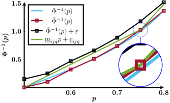
Figure 1: Quantile approximation method applied to a Cauchy distribution. The blue line represents the true quantile, the red points result from a Taylor series approximation (15), the black points show the error threshold $\xi$, and the green lines represent the affine approximation (19).

Algorithm 1 Computing $\{\underline{m}_{ijq},\underline{c}_{ijq}\}$ from $\phi_{\eta_{i}}$

Input: The PDF of $\eta_{i}$, $\phi_{\eta_{i}}$, and its derivatives $\phi^{{}^{\prime}}_{\eta_{i}},\ldots,\phi^{(n)}_{\eta_{i}}$, instantiating point $p_{0}$, termination point $p_{l}$, known quantile $\Phi^{-1}_{\eta_{i}}(p_{0})$, step size $h$, and maximum error threshold $\xi$.
Output: Affine terms of $\hat{\Phi}^{-1}_{\eta_{i}}$, $\{\underline{m}_{ijq},\underline{c}_{ijq}\}$

1:for $p_{i}=p_{0}+h$ to $p_{l}$ by $h$ do

2:     $\mathcal{P}_{i}\leftarrow\hat{\Phi}^{-1}(p_{i})$ $\triangleright$ Via (15)

3:end for

4:$i\leftarrow 0$

5:while $i<l$ do

6:     for $j=l$ to $i+1$ by $-1$ do

7:         $\underline{m}\leftarrow\frac{\mathcal{P}_{j}-\mathcal{P}_{i}}{h(j-i)}$

8:         $\underline{c}\leftarrow\mathcal{P}_{i}-p_{i}\times\underline{m}$

9:         for $y=i+1$ to $l-1$ by $1$ do

10:              $\epsilon_{y}=\mathcal{P}_{y}-(p_{y}\times\underline{m}+\underline{c})$

11:              if $\epsilon_{y}>\xi$ then next $j$

12:         end for

13:         $\{\underline{m}_{ijq},\underline{c}_{ijq}\}\leftarrow\underline{m},\underline{c}$

14:         Break

15:     end for

16:     $i\leftarrow j$

17:end while

We reformulate (14a) with the piecewise affine approximation (19), as

$$f_{i}(\overline{x}_{j}(0),\overline{U}_{j}) \leq c_{i}-\frac{1}{g_{i}}\left(\underline{s}_{ij}\right)$$ (20a)

$$\underline{s}_{ij} \geq\underline{m}_{ijq}\,\underline{\omega}_{ij}+\underline{c}_{ijq} \forall q\in\mathbb{N}_{[1,l^{\ast}]}$$ (20b)

$$\textstyle\sum_{j=1}^{v}\sum_{i=1}^{n_{j}}\underline{\omega}_{ij} \leq\alpha$$ (20c)

$$\underline{\omega}_{ij} \geq 0$$ (20d)

with slack variables $\underline{s}_{ij}$. A similar reformulation can be posed for (14d). In the limit, as (19) becomes an affine overapproximation of $\Phi^{-1}(\cdot)$, (20) is a tightening of (14) and Assumption 1 ensures the convexity of (20).

Lemma 2.

For a controller $\overline{U}_{1},\dots,\overline{U}_{v}$, if there exists risk allocation variables $\underline{\omega}_{ij}$ and $\underline{\beta}_{ij}$, and slack variables $\underline{s}_{ij}$ satisfying (20), then $\overline{U}_{1},\dots,\overline{U}_{v}$ asymptotically satisfies (7d) as $h\rightarrow 0$ and $n\rightarrow\infty$.

Proposed reformulation to solve Problem 1:

$$\underset{\begin{subarray}{c}\overline{U}_{1},\dots,\overline{U}_{v}\\ \overline{\omega}_{11},\dots,\overline{\omega}_{ij}\\ \overline{s}_{11},\dots,\overline{s}_{ij}\end{subarray}}{\mathrm{minimize}}\quad J\left(\bm{X}_{1},\ldots,\bm{X}_{v},\overline{U}_{1},\dots,\overline{U}_{v}\right)$$ (21a)

$$\mathrm{subject\ to}\quad \overline{U}_{1},\dots,\overline{U}_{v}\in\mathcal{U}^{N},$$ (21b)

$$\text{Dynamics \eqref{eq:lin_dynamics} with initial states }\overline{x}_{1}(0),\dots,\overline{x}_{v}(0)$$ (21c)

$$\forall j\in\mathbb{N}_{[1,v]},i\in\mathbb{N}_{[1,n_{j}]}\quad f_{i}(\overline{x}_{j}(0),\overline{U}_{j})\leq c_{i}-\frac{1}{g_{i}}\left(\underline{s}_{ij}\right) f_{i}(\overline{x}_{j}(0),\overline{U}_{j})\geq c_{i}+\frac{1}{g_{i}}\left(\underline{s}_{ij}\right)$$  and/or (21d)

$$\hskip 15.0pt\forall j\in\mathbb{N}_{[1,v]},i\in\mathbb{N}_{[1,n_{j}]},q\in\mathbb{N}_{[1,l^{\ast}]}\quad \underline{s}_{ij}\geq\underline{m}_{ijq}\,\underline{\omega}_{ij}+\underline{c}_{ijq} \underline{s}_{ij}\geq\underline{m}_{ijq}\,\underline{\beta}_{ij}+\underline{c}_{ijq}$$  and/or (21e)

$$\textstyle\sum_{j=1}^{v}\sum_{i=1}^{n_{j}}\underline{\omega}_{ij}\leq\alpha \textstyle\sum_{j=1}^{v}\sum_{i=1}^{n_{j}}\underline{\beta}_{ij}\leq\alpha$$  and/or (21f)

$$\forall j\in\mathbb{N}_{[1,v]},i\in\mathbb{N}_{[1,n_{j}]}\quad \underline{\omega}_{ij}\geq 0 \underline{\beta}_{ij}\geq 0$$  and/or (21g)

 

Proof.

By (18), the approximation error $\epsilon\rightarrow 0$ as $h\rightarrow 0$ and $n\rightarrow\infty$. In this case, (20) conservatively enforces (14) by (19). By Lemma 1, (7d) is conservatively enforced. ∎

We note that a limitation of our approach is that we can only guarantee constraint satisfaction in the limit. In practice, a sufficiently differentiable distribution will likely behave well enough that four or more derivatives will result in an approximation with small errors given a small enough step size. Many common distributions will fall into this category, especially those of the exponential family of distributions. Where this methodology will likely fail is multi-modal distributions or distributions that have a non-smooth terminating derivative. We have found empirically that a step size, $h$, on the order of $10^{-6}$, is sufficiently small that the approximation error, (17), is also on the order of $10^{-6}$.

III-C Reverse Convex Constraints

A standard approach to handling reverse convex constraints is difference of convex programming,

$$\begin{split}\underset{x}{\mathrm{minimize}}\quad&\mathcal{F}_{0}(x)-\mathcal{G}_{0}(x)\\ \mathrm{subject\ to}\quad&\mathcal{F}_{i}(x)-\mathcal{G}_{i}(x)\leq 0\quad\text{for }i\in\mathbb{N}_{[1,L]}\\ \end{split}$$ (22)

in which the cost and constraints are represented as the difference of two convex functions, i.e., $\mathcal{F}_{0},\mathcal{F}_{i}(\cdot):\mathbb{R}^{n}\rightarrow\mathbb{R}$ and $\mathcal{G}_{0},\mathcal{G}_{i}(\cdot):\mathbb{R}^{n}\rightarrow\mathbb{R}$ for $x\in\mathbb{R}^{n}$ are convex. The convex-concave procedure solves (22) to a local minimum [15] through an iterative approach, which employs first order approximations of $\mathcal{G}_{0},\mathcal{G}_{i}$ at each iteration. Feasibility of (22) is dependent on the feasibility of the initial conditions.

We can show that (14d) elicits a difference of convex formulation by subtracting $f_{i}(\overline{x}_{j}(0),\overline{U}_{j})$ from both sides. We also add slack variables to accommodate potentially infeasible initial conditions [15], [21]. When using a difference of convex program, Lemma 1 guarantees a feasible but locally optimal solution.

IV Experimental Results

We demonstrate our algorithms in simulation on a multi-vehicle spacecraft navigation problem with two disturbances: one that is Gaussian (for validation), and one that is Cauchy (to demonstrate our method’s capabilities). All computations were done on a 1.80GHz i7 processor with 16GB of RAM, using MATLAB, CVX [22] and Gurobi [23]. Polytopic construction and plotting was done with MPT3 [24]. The system formulations are implemented in SReachTools [25]. All code is available at https://github.com/unm-hscl/shawnpriore-approximate-quantiles.

Consider a scenario in which three satellites are stationed in low earth orbit. Each satellite is tasked with reaching a terminal target set, while avoiding other satellites. The relative dynamics of each spacecraft, with respect to a known and fixed origin, are described by the Clohessy-Wilthire-Hill (CWH) equations [26]

$$\ddot{x}-3\omega^{2}x-2\omega\dot{y} =\frac{F_{x}}{m_{c}}$$ (23a)

$$\ddot{y}+2\omega\dot{x} =\frac{F_{y}}{m_{c}}$$ (23b)

$$\ddot{z}+\omega^{2}z =\frac{F_{z}}{m_{c}}.$$ (23c)

with input $u_{i}=[\begin{array}[]{ccc}F_{x}&F_{y}&F_{z}\end{array}]^{\top}$, mass $m_{c}$, and orbital rate $\omega=\sqrt{\frac{\mu}{R^{3}_{0}}}$, with gravitational constant $\mu$ and orbital radius $R_{0}$. We discretize (23) with a first-order hold, with sampling time $30$$\mathrm{s}$, and insert a disturbance process that captures model uncertainties, so that dynamics for vehicle $i$ are described by

$$\bm{x}_{i}(k+1)=A\bm{x}_{i}(k)+B\overline{u}_{i}(k)+\bm{w}_{i}(k)$$ (24)

with $\mathcal{U}_{i}=[-5,5]^{3}$, and time horizon $N=8$, corresponding to 4 minutes of operation.

The terminal sets $\mathcal{T}_{i}$ are $5\times 5\times 5$m boxes centered around desired terminal locations in $x,y,z$ coordinates, with speeds bounded in all three directions by $[-0.01,0.01]$m/s. For collision avoidance, we presume that all satellites must remain at least $r=15$m away from each other, hence $S=\begin{bmatrix}I_{3}&0_{3}\end{bmatrix}$ to extract the positions. Violation thresholds for terminal sets and collision avoidance are $\alpha_{\mathcal{T}}=\alpha_{r}=0.1$, respectively.

$$\mathbb{P}\left\{\bigcap_{i=1}^{3}\bm{x}_{i}(N)\in\mathcal{T}_{i}\right\} \geq 1-\alpha_{\mathcal{T}}$$ (25)

$$\mathbb{P}\left\{\bigcap_{k=1}^{N}\bigcap_{i,j=1}^{3}\left\|S\!\cdot\!\left(\bm{x}_{i}(k)\!-\!\bm{x}_{j}(k)\right)\right\|\geq r\right\} \geq 1-\alpha_{r}$$ (26)

The performance objective is based on fuel consumption.

$$J(\overline{U}_{1},\overline{U}_{2},\overline{U}_{3})=\sum^{3}_{i=1}\overline{U}_{i}^{\top}\overline{U}_{i}$$ (27)

When approximating the numerical quantile, we presume intervals $h=5\times 10^{-6}$, and maximum approximation error $\xi=0.1$. For symmetric distributions, we set the instantiating point, $p_{0}$, to $0.5$ with known quantile $\Phi^{-1}(p_{0})=0$. For non-symmetric distributions, we set the instantiating point to $0.9$. Computation of $\Phi^{-1}(p_{0})$ was completed with MATLAB’s implementation of the incomplete gamma function for the Chi quantile. Analytical results were used to compute $\Phi^{-1}(p_{0})$ for the sum of squared Cauchy random variables. Each quantile approximation used the first three derivatives of the pdf. Convergence criteria was defined as the difference of sequential outputs and the sum of slack variables both less than $10^{-8}$; difference of convex programs were limited to 100 iterations.

IV-A 6D CWH with a Gaussian Disturbance

We first consider a Gaussian noise with zero mean and covariance $\Sigma=\mathrm{diag}(10^{-4}\cdot I_{3},5\times 10^{-8}\cdot I_{3})$. Once reformulated, the target set constraint has a Gaussian distribution and the collision avoidance has a Chi distribution with three degrees of freedom. As neither have an analytical expression for their quantile function, the use of standard tools or methods [14, 16] for Gaussian distributions is not viable.

For terminal constraint (25), formulation into (6a) via (36) results in $\eta_{i}$ that is a univariate Gaussian distribution with zero mean and variance $P_{i,\cdot}\,\Sigma(k)\,P_{i,\cdot}^{\top}$, with $\Sigma(k)=\sum_{i=0}^{k-1}(A^{i})^{\top}\Sigma A^{i}$, such that $g_{i}\eta_{i}=P_{i,\cdot}\,\Sigma(k)\,P_{i,\cdot}^{\top}\eta_{i}$.

For the collision avoidance constraint (26), formulation into (6b) via (39) follows the derivation as in [16, Thm 1], and results in

$$\begin{split}&\left\|S\!\left(\bm{x}_{i}(k)-\bm{x}_{j}(k)\right)\right\|\\ \equiv&\left\|S\!\left(A^{k}\overline{x}_{i-\!j}(0)+\mathcal{C}_{u}(k)\overline{U}_{i-\!j}+\mathcal{C}_{w}(k)\bm{W}_{i-\!j}\right)\right\|\\ \geq&\left\|S\!\left(A^{k}\overline{x}_{i-\!j}(0)+\mathcal{C}_{u}(k)\overline{U}_{i-\!j}\right)\right\|-\left\|S\mathcal{C}_{w}(k)\bm{W}_{i-\!j}\right\|\\ \geq&\underbrace{\left\|\vphantom{\left(2S\Sigma(k)S^{\top}\right)^{\frac{1}{2}}}S\!\left(A^{k}\overline{x}_{i-\!j}(0)+\mathcal{C}_{u}(k)\overline{U}_{i-\!j}\right)\right\|}_{f_{i}(\overline{x}(0),\overline{U})}\!-\!\underbrace{\left\|\left(2S\Sigma(k)S^{\top}\right)^{\frac{1}{2}}\bm{\rho}\right\|}_{g_{i}\eta_{i}}\end{split}$$ (28)

where the index $\cdot_{i-j}$ represents the difference between the two variables, respectively, and $\bm{\rho}$ is a multivariate Gaussian. By the compatibility of matrix norms, we obtain

$$g_{i}\eta_{i}=\left\|\left(2S\Sigma(k)S^{\top}\right)^{\frac{1}{2}}\right\|\cdot\left\|\bm{\rho}\right\|$$ (29)

where $\left\|\bm{\rho}\right\|$ follows a Chi distribution with three degrees of freedom.

We compare the proposed method with the mixed integer particle approach using two polytopic overapproximations of the collision avoidance constraint, based on the $L_{\infty}$ and $L_{1}$ norm. We generated 10 disturbance samples to generate an open-loop controller. Note that different disturbance samples were used when generating the controller for either variant.

The resulting trajectories, costs, and computation times differ dramatically, as shown in Figure 2 and Table I. (Differences in the $z$-coordinates were minimal, so we only plot the $x$ and $y$ coordinates in Figure 2.) To assess constraint satisfaction, we generated $10^{5}$ Monte-Carlo sample disturbances for each approach; the the $L_{2}$ distance between the mean positions at each time step are shown in Figure 3. Table II shows that while all three methods satisfied the collision avoidance constraint, neither particle control approach satisfied the terminal set constraint.

The proposed method performed two to three orders of magnitude faster than particle control. Given the significant increase in binary variables needed to perform particle control, this comes as no surprise. We attempted to increase the number of disturbance samples, however, we could not generate a solution in a under two hours. Conversely, the low number of disturbance samples is likely the cause for the poor performance with respect to the target set constraint. Given the random nature of the sampling process, ten samples is not enough to characterize the behaviour on a larger scale.

Figures 2 and 3 show that the differences in avoidance regions impacted the results. With the $L_{2}$ collision avoidance region overapproximated by both the $L_{\infty}$ and $L_{1}$ regions, we

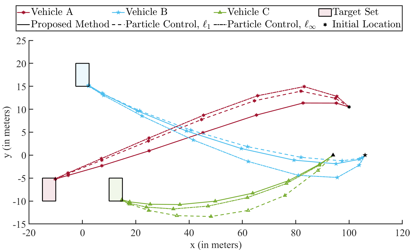
Figure 2: Comparison of trajectories in $(x,y)$ coordinates from proposed method (solid) and particle control (dashed for $L_{1}$ norm; dotted for $L_{\infty}$ norm).

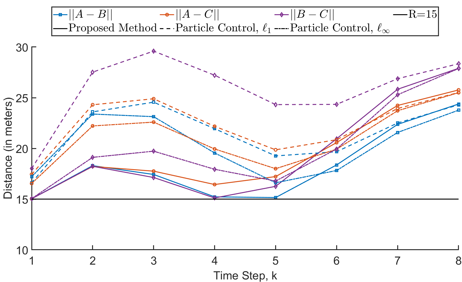
Figure 3: Comparison of $L_{2}$ inter-satellite distances between proposed method (solid) and particle control (dashed for $L_{1}$ norm; dotted for $L_{\infty}$ norm).

TABLE I: Computation Time and Control Cost for CWH Dynamics with a Gaussian Disturbance.

Metric	Proposed method	Particle control
		$L_{\infty}$	$L_{1}$
Computation Time (sec)	6.82	245.65	4199.10
$J(\overline{U}_{1},\overline{U}_{2},\overline{U}_{3})$	92.04	102.79	117.56

TABLE II: Constraint Satisfaction (”SAT”) for CWH dynamics with Gaussian Disturbance, with $10^{5}$ Samples and Probabilistic Violation Threshold of $1-\alpha=0.9$.

Constraint	Proposed method	SAT	Particle control
			$L_{\infty}$	SAT	$L_{1}$	SAT
Collision Avoidance	0.9630	$\checkmark$	0.9997	$\checkmark$	1.0000	$\checkmark$
Terminal Set	0.9127	$\checkmark$	0.2183		0.0993

expected the collision avoidance likelihood to be significantly higher than the proposed method. However, the sharp edges of the polytopes created control choices that led to more aggressive direction changes. This phenomena is apparent in the lack of smoothness in the particle control trajectories in Figure 2. Similarly, the larger avoidance regions effectively increased the avoidance distance to $18$\mathrm{m}$$ for the $L_{\infty}$ particle control run and $23$\mathrm{m}$$ for the $L_{1}$ particle control run, as observed in Figure 3. The additional distance had a distinct impact on the overall cost of each of these controllers. To produce a closer comparison, we also used 14- and 26-faced polytopes, however neither resulted in a solution within a $24$ hour time frame.

IV-B 4D CWH with Cauchy Disturbance

We consider the planar CWH dynamics (23a), (23b) with a Cauchy disturbance that is parameterized with location as zero and scale elements $\Gamma(k)$,

$$\Gamma(k)_{j}=\begin{cases}10^{-4}&\text{if }j\in\{4n+\{1,2\}\mid n\in\mathbb{N}_{[0,k-1]}\}\\ 5\!\times\!10^{-8}&\text{if }j\in\{4n+\{3,4\}\mid n\in\mathbb{N}_{[0,k-1]}\}\end{cases}$$ (30)

corresponding to position and velocity elements, respectively.

For the terminal set constraint, because the set is axis-aligned, it can be written as function of a single Cauchy random variable,

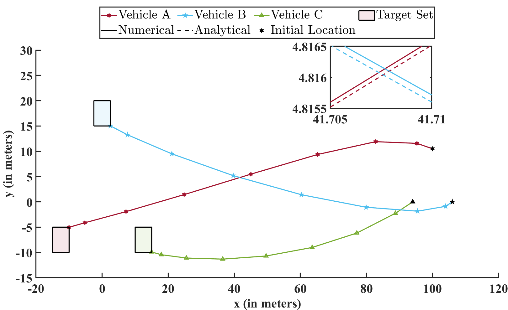
Figure 4: Comparison of trajectories in $(x,y)$ coordinates for proposed method (solid) and with an analytic quantile (dashed). The trajectories are nearly indistinguishable as seen in the magnified subplot.

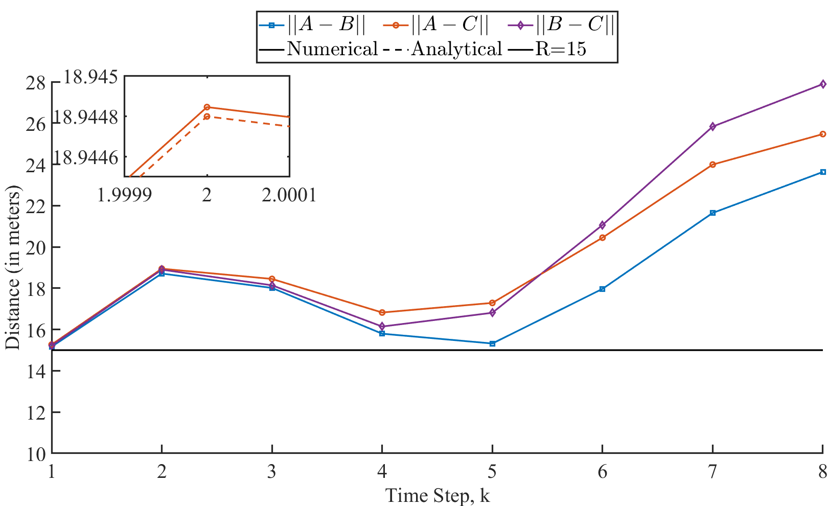
Figure 5: Comparison of inter-satellite distances between proposed method (solid) and with an analytic quantile (dashed). The inter-satellite distances are nearly indistinguishable as seen in the magnified subplot.

$$\begin{array}[]{rrl}&\overline{e}_{m}^{\top}\,\bm{x}_{j}&\leq\overline{q}_{i}\\ \Leftrightarrow&\underbrace{\overline{e}_{m}^{\top}\left(A^{k}\overline{x}_{j}(0)+\mathcal{C}_{u}(k)\overline{U}_{j}\right)}_{f_{i}(\overline{x}_{j}(0),\overline{U}_{j})}\!+\!\underbrace{\,\overline{e}_{m}^{\top}\,\mathcal{C}_{w}(k)\bm{W}}_{g_{i}\eta_{i}}&\leq\underbrace{\overline{q}_{i}}_{c_{i}}\end{array}$$ (31)

where $\overline{e}_{m}$ is the $m$-th column of an appropriately sized identity matrix. Here,

$$g_{i}\eta_{i}=\overline{e}_{m}^{\top}\mathcal{C}_{w}(k)\Gamma(k)\eta_{i}\\$$ (32)

and $\eta_{i}$ has a standard Cauchy distribution. Note that without a direct covariance measure between two Cauchy distributions, (31) cannot be easily extended to account for polytopic constraints of more than one dimension.

For the collision avoidance constraint, the main challenge arises from the coupling across random variables that arises from taking a norm. By falsely considering each dimension as independent, we under approximate the norm

$$\left\|S\!\left(\bm{x}_{i}(k)-\bm{x}_{j}(k)\right)\right\|$$ (33)

$$\equiv \left\|S\!\left(A^{k}\overline{x}_{i-\!j}(0)\!+\!\mathcal{C}_{u}(k)\overline{U}_{i-\!j}+\mathcal{C}_{w}(k)\bm{W}_{i-\!j}\right)\right\|$$

$$\geq \left\|S\!\left(A^{k}\overline{x}_{i-\!j}(0)\!+\!\mathcal{C}_{u}(k)\overline{U}_{i-\!j}\right)\right\|\!-\!\left\|S\mathcal{C}_{w}(k)\bm{W}_{i-\!j}\right\|$$

$$\geq \underbrace{\left\|S\!\left(A^{k}\overline{x}_{i-\!j}(0)\!+\!\mathcal{C}_{u}(k)\overline{U}_{i-\!j}\right)\right\|}_{f_{i}(\overline{x}(0),\overline{U})}\!-\!\underbrace{\mathrm{max}\left(S\mathcal{C}_{w}(k)\Gamma(k)\right)\left\|\bm{\rho}\right\|}_{g_{i}\eta_{i}}$$

where $\bm{\rho}$ is a 2D vector consisting of independent and identically distributed standard Cauchy variables, and $\mathrm{max}(\cdot)$ returns the element of the argument vector with the maximum value. Note that the random variable of interest is $\left\|\bm{\rho}\right\|^{2}$, which we can show through convolution to have closed-form expressions for the pdf, cdf, and the quantile,

$$\phi_{\left\|\bm{\rho}\right\|^{2}}(x) =\frac{2}{\pi\sqrt{1+x}(2+x)}$$ (34a)

$$\Phi_{\left\|\bm{\rho}\right\|^{2}}(x) =\textstyle\frac{4}{\pi}\arctan\left(\sqrt{1+x}\right)-1$$ (34b)

$$\Phi^{-1}_{\left\|\bm{\rho}\right\|^{2}}(p) =\tan^{2}\left(\textstyle\frac{\pi}{4}(1+p)\right)-1$$ (34c)

Figures 4 and 5, and Tables III and IV, show that the proposed method with the numerical quantile performed nearly identically to the proposed method with an analytical quantile. We observed differences on the order of $10^{-4}$, as shown in the subplot of Figure 4. This is likely attributed to

TABLE III: Computation Time and Control Cost for CWH Dynamics with Cauchy Disturbance.

Metric	Proposed method
	Numerical	Analytical
Computation Time (sec)	153.86	157.98
$J(\overline{U}_{1},\overline{U}_{2},\overline{U}_{3})$	93.11	93.11

TABLE IV: Constraint Satisfaction (“SAT”) for CWH dynamics with Cauchy Disturbance, with $10^{5}$ Samples and Probabilistic Violation Threshold of $1-\alpha=0.9$.

Constraint	Proposed method
	Numerical	SAT	Analytical	SAT
Collision Avoidance	0.9979	$\checkmark$	0.9978	$\checkmark$
Terminal Set	0.9086	$\checkmark$	0.9085	$\checkmark$

our choice of a very small interval $h$, which yielded a highly accurate quantile approximation.

V Conclusion

We proposed a method for chance constrained stochastic optimal control of LTI systems that exploits a numerical approximation of the quantile function. Our approach is amenable to distributions whose pdfs are sufficiently smooth. We demonstrated our approach on a multi-vehicle satellite control problem with Gaussian and Cauchy disturbances.

-A Reformulation of Constraints

-A1 Polytopic constraint set

Consider a terminal set constraint, captured by (4a) as

$$\mathbb{P}\{\bm{x}(N)\in\mathcal{T}_{N}\}\geq 1-\alpha,$$ (35)

whose argument can be rewritten in halfspace form as $P\bm{x}_{j}(N)\leq\overline{p}$ for some $P\in\mathbb{R}^{L\times n}$, $\overline{p}\in\mathbb{R}^{L}$, for $L$ the number of half-space constraints in $\mathcal{T}_{k}$. Expanding into an intersection of scalar constraints, we obtain

$$\begin{array}[]{rrl}&P\bm{x}_{j}(k)&\leq\overline{p}\\ \Leftrightarrow&\displaystyle\bigcap_{i=1}^{L}P_{i,\cdot}\bm{x}_{j}(k)&\leq\overline{p}_{i}\\ \Leftrightarrow\!&\!\displaystyle\bigcap_{i=1}^{L}\underbrace{P_{i,\cdot}\left(A^{k}\overline{x}_{j}(0)+\mathcal{C}_{u}(k)\overline{U}_{j}\right)}_{f_{i}(\overline{x}_{j}(0),\overline{U}_{j})}+\underbrace{P_{i,\cdot}\,\mathcal{C}_{w}(k)\bm{W}}_{g_{i}\eta_{i}}&\leq\underbrace{\overline{p}_{i}}_{c_{i}}\end{array}$$ (36)

where $P_{i,\cdot}$ is the $i^{\text{th}}$ row of the matrix $P$, meaning that

$$\mathbb{P}\{\bm{x}(N)\in\mathcal{T}_{N}\}\geq 1-\alpha\Leftrightarrow\>\mathbb{P}\>\left\{\eqref{eq:demo1}\right\}\geq 1-\alpha$$ (37)

as in (6a), with random variable $\eta$ that is a linear transformation of $w$.

-A2 Norm based constraint set

For probabilistic collision avoidance between vehicles $i$ and $j$ with minimum $L_{2}$ distance $r\in\mathbb{R}_{+}$ and violation threshold $1-\alpha$, we consider

$$\mathbb{P}\{\|\bm{x}_{i}(k)-\bm{x}_{j}(k)\|\geq r\}\geq 1-\alpha$$ (38)

Using the reverse triangle inequality, we obtain

$$\|\bm{x}_{i}(k)-\bm{x}_{j}(k)\|$$ (39a)

$$= \|A^{k}[\overline{x}_{i}(0)\!-\!\overline{x}_{j}(0)]\!+\!\mathcal{C}_{u}(k)[\overline{U}_{i}\!-\!\overline{U}_{j}]\!+\!\mathcal{C}_{w}(k)(\bm{W}_{i}\!-\!\bm{W}_{j})\|$$ (39b)

$$\geq \underbrace{\|A^{k}[\overline{x}_{i}(0)\!-\!\overline{x}_{j}(0)]\!+\!\mathcal{C}_{u}(k)[\overline{U}_{i}\!-\!\overline{U}_{j}]\|}_{f_{i}(\overline{x}_{j}(0),\overline{U}_{j})}\!-\!\underbrace{\|\mathcal{C}_{w}(k)(\bm{W}_{i}\!-\!\bm{W}_{j})\|}_{g_{i}\eta_{i}}$$ (39c)

hence

$$\mathbb{P}\{\|\bm{x}_{i}(k)-\bm{x}_{j}(k)\|\geq r\}\geq 1-\alpha\\ \Leftarrow\mathbb{P}\{\eqref{eq:demo_2_final}\geq r\}\geq 1-\alpha$$ (40)

as in (6b). Note that this is a one-way implication.

References

- [1] A. Mesbah, “Stochastic model predictive control: An overview and perspectives for future research,” IEEE Ctrl. Syst. Mag., vol. 36, no. 6, pp. 30–44, 2016.
- [2] G. Calafiore and M. Campi, “The scenario approach to robust control design,” IEEE Trans. Autom. Control, vol. 51, no. 5, pp. 742–753, 2006.
- [3] L. Blackmore, M. Ono, and B. Williams, “Chance-constrained optimal path planning with obstacles,” IEEE Trans. Robot., vol. 27, no. 6, pp. 1080–1094, 2011.
- [4] M. Campi and S. Garatti, “A sampling-and-discarding approach to chance-constrained optimization: Feasibility and optimality,” J. Optim Theory Appl., vol. 148, no. 2, pp. 257–280, 2011.
- [5] A. Carè, S. Garatti, and M. C. Campi, “Fast—fast algorithm for the scenario technique,” Operations Res., vol. 62, no. 3, pp. 662–671, 2014.
- [6] M. C. Campi, S. Garatti, and F. A. Ramponi, “A general scenario theory for nonconvex optimization and decision making,” IEEE Transactions on Automatic Control, vol. 63, no. 12, pp. 4067–4078, 2018.
- [7] A. Nemirovski and A. Shapiro, “Convex approximations of chance constrained programs,” J. Optimization, vol. 17, pp. 969–996, 2006.
- [8] G. Calafiore and L. Ghaoui, “On distributionally robust chance-constrained linear programs,” J. Optim Theory Appl., vol. 130, no. 1, pp. 1–22, 2006.
- [9] J. Paulson, E. Buehler, R. Braatz, and A. Mesbah, “Stochastic model predictive control with joint chance constraints,” Int’l J. Ctrl., pp. 1–14, 2017.
- [10] F. Oldewurtel, C. Jones, A. Parisio, and M. Morari, “Stochastic model predictive control for building climate control,” IEEE Trans. Control Syst. Technol., vol. 22, no. 3, pp. 1198–1205, 2014.
- [11] M. Ono and B. Williams, “Iterative risk allocation: A new approach to robust model predictive control with a joint chance constraint,” in IEEE Conf. Dec. & Control, pp. 3427–3432, 2008.
- [12] M. P. Vitus and C. J. Tomlin, “On feedback design and risk allocation in chance constrained control,” in 2011 50th IEEE Conference on Decision and Control and European Control Conference, pp. 734–739, 2011.
- [13] V. Sivaramakrishnan, A. P. Vinod, and M. Oishi, “Convexified open-loop stochastic optimal control for linear non-gaussian systems,” arXiv:2010.02101, 2021.
- [14] A. P. Vinod, V. Sivaramakrishnan, and M. Oishi, “Piecewise-affine approximation-based stochastic optimal control with gaussian joint chance constraints,” in Proc. Amer. Ctrl. Conf., pp. 2942–2949, 2019.
- [15] T. Lipp and S. Boyd, “Variations and extension of the convex–concave procedure,” Optimization and Eng., vol. 17, pp. 263––287, 2016.
- [16] S. Priore, A. Vinod, V. Sivaramakrishnan, C. Petersen, and M. Oishi, “Stochastic multi-satellite maneuvering with constraints in an elliptical orbit,” in Proc. Amer. Ctrl. Conf., pp. 4261–4268, 2021.
- [17] M. Abramowitz and I. A. Stegun, Handbook of mathematical functions with formulas, graphs, and mathematical tables, vol. 55. US Government printing office, 1964.
- [18] K. Kafadar and J. W. Tukey, “A bidec t table,” Journal of the American Statistical Association, vol. 83, no. 402, pp. 532–539, 1988.
- [19] M. J. Wichura, “Algorithm as 241: The percentage points of the normal distribution,” Journal of the Royal Statistical Society. Series C (Applied Statistics), vol. 37, no. 3, pp. 477–484, 1988.
- [20] C. Yu and D. Zelterman, “A general approximation to quantiles,” Communications in Statistics - Theory and Methods, vol. 46, no. 19, pp. 9834–9841, 2017.
- [21] R. Horst, P. M. Pardalos, and N. V. Thoai, Introduction to global optimization. Springer Science & Business Media, 2000.
- [22] M. Grant and S. Boyd, “CVX: Matlab software for disciplined convex programming, version 2.1.” http://cvxr.com/cvx, Mar. 2014.
- [23] L. Gurobi Optimization, “Gurobi optimizer reference manual,” 2020.
- [24] M. Herceg, M. Kvasnica, C. Jones, and M. Morari, “Multi-Parametric Toolbox 3.0,” in Proc. Euro. Ctrl. Conf., (Zürich, Switzerland), pp. 502–510, July 17–19 2013.
- [25] A. Vinod, J. Gleason, and M. K. Oishi, “SReachTools: A MATLAB Stochastic Reachability Toolbox,” in Proc. Hybrid Sys.: Comp. & Ctrl, pp. 33 – 38, April 2019. https://sreachtools.github.io.
- [26] W. Wiesel, Spaceflight Dynamics. New York: McGraw-Hill, 1989.