Predictability and Fairness in Load Aggregation
and Operations of Virtual Power Plants
Abstract
In power systems, one wishes to regulate the aggregate demand of an ensemble of distributed energy resources (DERs), such as controllable loads and battery energy storage systems. We suggest a notion of predictability and fairness, which suggests that the long-term averages of prices or incentives offered should be independent of the initial states of the operators of the DER, the aggregator, and the power grid. We show that this notion cannot be guaranteed with many traditional controllers used by the load aggregator, including the usual proportional-integral (PI) controller. We show that even considering the non-linearity of the alternating-current model, this notion of predictability and fairness can be guaranteed for incrementally input-to-state stable (iISS) controllers, under mild assumptions.
Index Terms:
Demand-side management, Load management, Power demand, Power systems, Power system analysis computing.I Introduction
In response to large-scale integration of intermittent sources of energy [1] in power systems, system operators seek novel approaches to balancing the load and generation. The aggregation of distributed energy resources (DERs) and regulation of their aggregate power output has emerged as a viable balancing mechanism [2, 3, 4, e.g.] for many system operators.111 In Australia, for instance, it is estimated that there are 2.5 million rooftop solar installations with a total capacity of more than 10 GW and 73,000 home energy storage systems with a 1.1 GW capacity.
For the transmission system operator, the load aggregator provides a single point of contact, which is responsible for the management of risks involved in the coordination of an ensemble of DERs and loads, and the legal and accounting aspects associated with modern grid codes and contracts governing the provision of ancillary services to the grid.
The load aggregator then coordinates an ensemble of participants, which can take many forms, including DERs [5, e.g.], interruptible or deferrable loads [6, 7, e.g.], and eventually, vehicle-to-grid (V2G) services [8, 9, e.g.]. Load aggregation is sometimes also known as a virtual power plant [10, 11, 12].
Independent of the form of the ensemble, load aggregation introduces a novel feedback loop [13, 14] into regulation problems in power systems. Recent regulation222In the European Union, Regulation (EU) 2019/943 of the European Parliament and of the Council of 5 June 2019 on the internal market for electricity sets “fundamental principles [to] facilitate aggregation of distributed demand and supply”, while requiring “non-discriminatory market access” and “fair rules”. Its implementation in individual member states varies and is still in progress in many member states since mid-2021. mandates the use of load aggregation, and hence makes the closed-loop analysis of load aggregation very relevant. A recent pioneering study of the closed-loop aspects of load aggregation by Li et al. [14] leaves three issues open: how to go beyond a linearisation of the physics of the alternating-current (AC) model? How to model the uncertainty inherent in response to the control signal provided by the load aggregator? Finally, what criteria of a good-enough behaviour of such a closed-loop system to consider? The first issue is particularly challenging: While the consideration of losses in the AC model may be necessary [15] for the sake of the accuracy of the model, it introduces a wide range of challenging behaviours [16, 17] in the non-linear dynamics.
In this paper, we address all three issues in parallel. First, we suggest that good-enough behaviour involves “predictability and fairness” properties that are rarely considered in control theory and require new analytical tools. These include:
-
(a)
whether each DER and load, on average, receives similar treatment in terms of load reductions, disconnections, or power quality,
-
(b)
whether the prices or incentives depend on initial conditions, such as consumption at some point in the past,
-
(c)
whether the prices, incentives, or limitations of service are stable quantities, preferably not sensitive to noise entering the system, and predictable.
Building upon the recent work of [18], we show that these criteria can be phrased in terms of properties of a specific stochastic model. In particular, these criteria are achieved whenever one can guarantee the existence of the unique invariant measure of a stochastic model of the closed-loop system. Thus, the design of feedback systems for deployment in the demand-response application should consider both the traditional notions of regulation and optimality and provide guarantees concerning the existence of the unique invariant measure.
Next, we show that many familiar control strategies, in straightforward situations, do not necessarily give rise to feedback systems that possess the unique stationary measure. In theory, we use the model of [18] to show that with any controller that is linear marginally stable with a pole on the unit circle, where is a rational number, the closed-loop system cannot have a unique invariant measure. In practice, we illustrate this behaviour in simulations using Matpower [19].
As our main result, we show that one can design controllers that allow for predictability and fairness from the point of view of a participant, such as an operator of DERs, even in the presence of losses in the AC model. These results are based on a long work history on incremental input-to-state stability, which we have extended to a stochastic setting.

II Related Work
There is a rich history of work on dynamics and control in power systems, summarised in several excellent textbooks of [20, 21, 22, 17], and [23]. Without aiming to present a comprehensive overview, one should like to point out that traditionally, load frequency control (LFC) is performed using controllers with poles on the unit circle, such as proportional-integral (PI) controllers [24, 25, e.g.]. There are many alternative proposals, some of them excellent [26, 27, 28, 29, 30, 31, 32, 33, 34, e.g.], but even the most recent textbook of [23, Chapter 4, “Robust PI-Based Frequency Control”] suggests that “complex state feedback or higher-order dynamic controllers […] are impractical for [the] industry”.
Although the idea of demand response has been studied for several decades [35, e.g.], only recently it has been shown to have commercial potential [36, 37, 38, 39]. Notably, with a capacity as low as 20–70 kWh, load aggregators may break even [39] in the spot market in developed economies, although many grid codes still require load aggregators to aggregate a substantially more enormous amount of active power (e.g., 1 MW).
Correspondingly, there has been much interest in incorporating load aggregation in load frequency control [40, 41, 42, 43, 44, 45, 46, 47, 48, 49, 50, 51, 52, 53, 54, 55]. We refer to [56] for a recent survey.
In a recent pioneering study, Li et al. [14] considered the closed-loop system design while quantifying the available flexibility from the aggregator to the system operator, albeit without the non-linearity of the alternating-current model.
III Notation, Preliminaries and Our Model
Let us introduce some definitions and notation:
Definition 1.
A function is is said to be of class if it is continuous, increasing and . It is of class if, in addition, it is proper, i.e., unbounded.
Definition 2.
A continuous function is said to be of class , if for all fixed the function is of class and for all fixed , the function is is non-increasing and tends to zero as .
In keeping with [18], our model is based on a feedback signal sent to agents. Each agent has a state and an associated output , where the latter is a finite set. The non-deterministic response of agent is within a finite set of actions: . The finite set of possible resource demands of agent is :
| (1) |
We assume there are state transition maps , for agent and output maps , for each agent . The evolution of the states and the corresponding demands then satisfy:
| (2) | ||||
| (3) |
where the choice of agent ’s response at time is governed by probability functions , , respectively , . Specifically, for each agent , we have for all that
| (4a) | ||||
| (4b) | ||||
| Additionally, for all , it holds that | ||||
| (4c) | ||||
The final equality comes from the fact , are probability functions. We assume that, conditioned on , the random variables are stochastically independent. The outputs each depend on and the signal only.
Let be a closed subset of with the usual Borel -algebra . We call the elements of events. A Markov chain on is a sequence of -valued random vectors with the Markov property, which is the equality of a probability of an event conditioned on past events and probability of the same event conditioned on the current state, i.e., we always have
where is an event and . We assume the Markov chain is time-homogeneous. The transition operator of the Markov chain is defined for , by
| (5) |
If the initial condition is distributed according to an initial distribution , we denote by the probability measure induced on the path space, i.e., space of sequences with values in . Conditioned on an initial distribution , the random variable is distributed according to the probability measure which is determined inductively by and
| (6) |
for .
A probability measure is called invariant with respect to the Markov process if it is a fixed point for the iteration described by (6), i.e., if
| (7) |
An invariant probability measure is called attractive, if for every probability measure the sequence defined by (6) with initial condition converges to in distribution.
In an iterated function systems with place dependent probabilities [60, 61, 62], we are given a set of maps , where is a (finite or countably infinite) index set. Associated to these maps, there are probability functions
| (8) |
The state at time is then given by with probability , where is the state at time . Sufficient conditions for the existence of a unique attractive invariant measure can be given in terms of “average contractivity” [57, 58, 59]. Any discrete-time Markov chain can be generated by an iterated function system with probabilities see Kifer[63, Section 1.1] or [64, Page 228], although such representation is not unique, see, Stenflo [65]. Although not well known, iterated function systems (IFS) are a convenient and rich class of Markov processes. The class of stochastic systems arising from the dynamics of multi-agent interactions can be modelled and analysed using IFS in a particularly natural way. A wealth of results[60, 66, 62, 67, 68, 69, 70, 71, 72, 73, 74, 75] then applies.
IV The Closed-Loop Model as Iterated Random Functions
Let us now model the system of Figure 1 by a Markov chain on a state space representing all the system components. In general, one could consider:
| (11) | ||||
| (12) |
| (13) |
| (14) |
In addition, we have (e.g., Dini) continuous probability functions so that the probabilistic laws (4) are satisfied. If we denote by and the state spaces of the agents, the controller and the filter, then the system evolves on the overall state space according to the dynamics
| (15) |
where each of the maps is of the form
| (16) |
and the maps are indexed by indices from the set
| (17) |
By the independence assumption on the choice of the transition maps and output maps for the agents, for each multi-index in this set, the probability of choosing the corresponding map is given by
| (18) |
We have obtained an iterated function system of the previous subsection III.
IV-A Our Objective
We aim to achieve regulation, with probability
| (19) |
to some reference , given by the installed capacity. Further, we aim for predictability, in the sense that for each agent there exists a constant such that
| (20) |
where the limit is independent of initial conditions. This can be guaranteed, when one has a unique invariant measure for the closed-loop model as iterated random functions. The requirement of fairness is then for the limit to coincide for all .
IV-B A Motivating Negative Result
The motivation for our work stems from the fact that controllers with integral action [76, 77], such as the Proportional-Integral (PI) controller, fail to provide unique ergodicity, and hence the fairness properties. In many applications, controllers with integral action are widely adopted, including leading control systems [78] in power generation. A simple PI control can be implemented as:
| (21) |
which means its transfer function from to , in terms of the transform, is given by
| (22) |
Since this transfer function is not asymptotically stable, any associated realisation matrix will not be Schur. Note that this is the case for any controller with any sort of integral action, i.e., a pole at .
Theorem 1 ([18]).
Consider agents with states . Assume that there is an upper bound on the different values the agents can attain, i.e., for each we have for a given set and .
Consider the feedback system in Figure 1, where is a finite-memory moving-average (FIR) filter. Assume the controller is a linear marginally stable single-input single-output (SISO) system with a pole on the unit circle where is a rational number, is the imaginary unit, and is Archimedes’ constant . In addition, let the probability functions be continuous for all , i.e., if is the output of at time , then . Then the following holds.
-
(i)
The set of possible output values of the filter is finite.
-
(ii)
If the real additive group generated by with from (19) is discrete, then the closed-loop system cannot be uniquely ergodic.
-
(iii)
For rational for all , , and rational coefficients of the FIR filter , the closed-loop system cannot be uniquely ergodic.
This suggests that it is perfectly possible for the closed loop both to perform its regulation function well and, at the same time, to destroy the ergodic properties of the closed loop. We demonstrate this in a realistic load-aggregation scenario in Section VI.
V The Main Result
For a linear controller and filter, [18] have established conditions that assure the existence of a unique invariant measure for the closed-loop. Let us consider non-linear controllers and filters, as required in power systems, and seek unique ergodicity conditions. Incremental stability is well-established concept to describe the asymptotic property of differences between any two solutions. One can utilise the concept of incremental input-to-state stability, which is defined as follows:
Definition 3 (Incremental ISS, [79]).
Let denote the set of all input functions . Suppose, is continuous, then the discrete-time non-linear dynamical system
| (23) |
is called (globally) incrementally input-to-state-stable (incrementally ISS), if there exist and such that for any pair of inputs and any pair of initial condition :
Definition 4 (Positively Invariant Set).
A set is called positively invariant under the system (23) if for any initial state we have .
Definition 5 (Uniform Exponential Incremental Stability).
The system (23) is uniformly exponentially incrementally stable in a positively invariant set if there exists and such that for any pair of initial states , for any pair of , and for all the following holds
| (24) |
If , then the system (23) is called uniformly globally exponentially incrementally stable.
With this notation, we can employ contraction arguments for iterated function systems [58] to prove:
Theorem 2.
Consider the feedback system depicted in Figure 1. Assume that each agent has a state governed by the non-linear iterated function system
| (25) | ||||
| (26) |
where:
-
(i)
we have globally Lipschitz-continuous and continuously differentiable functions and with global Lipschitz constant , resp.
-
(ii)
we have Dini continuous probability functions so that the probabilistic laws (4) are satisfied
-
(iii)
there are scalars such that , for all and all
-
(iv)
the composition (16) of agents’ transition maps and the probability functions satisfy the contraction-on-average condition. Specifically, consider the space of all agents and the maps , together with the probabilities , , form an average contraction system in the sense that there exists a constant such that for all we have
(27)
Then, for every incrementally input-to-state stable controller and every incrementally input-to-state stable filter compatible with the feedback structure, the feedback loop has a unique, attractive invariant measure. In particular, the system is uniquely ergodic.
Proof.
To prove the result, we have to show that the assumptions of Theorem 2.1 in [58] are satisfied. To this end, we note that the maps satisfy, by (i), the necessary Lipschitz conditions. Further, the probability maps have the required regularity and positivity properties by (ii) and (iii). Thus, it only remains to show that the maps defined in (16) have the average contraction property. The existence of a unique attractive invariant measure then follows from [58] and unique ergodicity follows from [57].
First we note that the filter and the controller are incrementally stable systems that are in cascade. It is shown in [79, Theorem 4.7] that cascades of incrementally ISS systems are incrementally ISS. The proof is given for continuous-time systems but readily extends to the discrete-time case. It will therefore be sufficient to treat filter and controller together as one system with state .
To show the desired contractivity property, consider two distinct points . Let be an upper bound for the Lipschitz constants of the output functions , . The assumptions on incremental ISS ensure that for each index
As the maps satisfy the average contractivity condition, it is an easy exercise to see that also the sets of iterates satisfy the contractivity condition. The result then can be obtained using Theorem 15 of [80], where it is shown that incrementally stable systems are contractions, using the converse Lyapunov theorem of [81]. The proof is concluded by invoking Theorem 2.1 in [58]. ∎
Subsequently, one may wish to design a controller that is a priori incrementally input-to-state-stable, e.g. considering extending the work on ISS-stable model-predictive controller [82] or model-predictive controllers [28, 29, 30, 31, 32, 33, 34] that are constrained to be small-signal stable. Alternatively, one may ask whether other controllers guaranteeing fairness are available, without explicitly adding incrementally input-to-state-stable constraints. The implementation depends on the setting under consideration.
VI Numerical results
Our numerical results are based on simulations utilising Matpower [19], a standard open-source toolkit for power-systems analysis in version 7.1 running on Mathworks Matlab 2019b. We use Matpower’s power-flow routine to implement a non-linear filter, which models the losses in the alternating-current model.
The model consists of an ensemble of DERs or partially-controllable loads divided into two groups that differ in their probabilistic response to the control signal provided by the load aggregator. In particular, following the closed-loop of Figure 1: The response of each system to the control signal provided by the load aggregator at time takes the form of probability functions, which suggest the probability a DERs is committed at time as a function of the control signal . In our simulations, the two functions satisfying (8) are:
| (28) | ||||
| (29) |
where we have implemented both PI and its lag approximant for the control of an ensemble of DERs or partially-controllable loads. The binary-valued vector:
| (30) |
captures the output of the probability functions (28) in a particular realization.
The commitment of the DERs within the ensemble is provided to Matpower, which using a standard power-flow algorithm computes the active power output of the individual DERs:
| (31) |
which is aggregated into the total active power output of the ensemble. Then, a filter is applied:
| (32) |
Notice that here we both smooth the total active power output with a moving-average filter and accommodate the losses in the AC model. The error
| (33) |
between the reference power output and the filtered value is then used as the input for the controller. Output of the controller is a function of error and an inner state of the controller . Signal of the controller is given by the PI or its lag approximant:
| (34) | ||||
| (35) |
The procedure is demonstrated in the following pseudocode.
VI-A A Serial Test Case
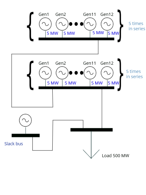
First, let us consider a simple serial test case depicted in Figure 2, where there are a number of buses connected in series, as they often are in distribution systems. In particular, the buses are:
-
•
a slack bus, such as a distribution substation,
-
•
5 buses with 12 DERs of 5 MW capacity connected to each bus, with probability function of (28) modelling the response of these first 60 DERs to the signal,
-
•
5 buses with 12 DERs of 5 MW capacity connected to each bus, with probability function of (28) modelling the response of these 60 DERs to the signal,
-
•
a single load bus with a demand of 500 MW.
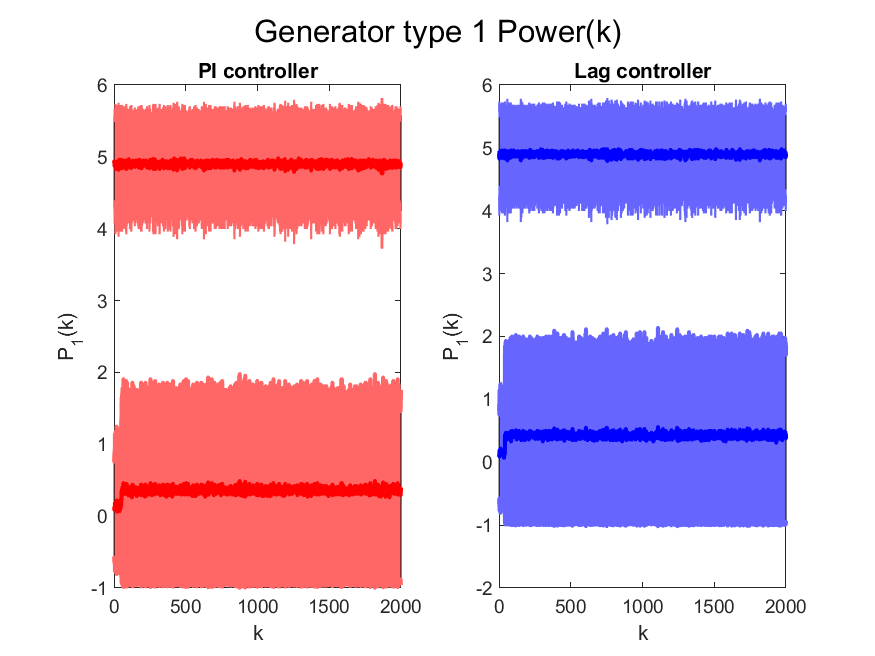
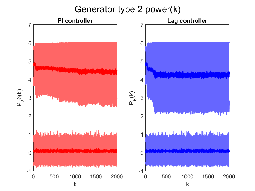
We aim to regulate the system to the reference signal , which is MW plus losses at time . Initially, the first 60 () generators are off and the second following 60 () generators are on. Considering the ensemble is composed of 120 DERs, with a total capacity of 600 MW, this should yield a load of less than 200 MW on the slack bus.
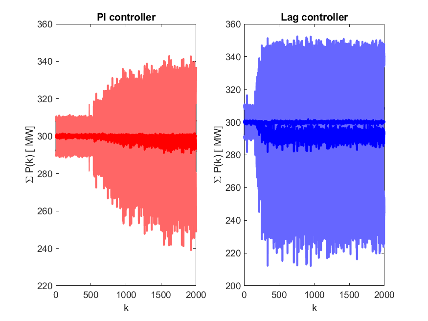
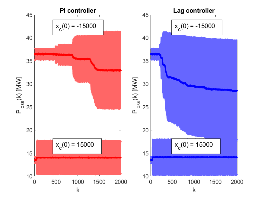
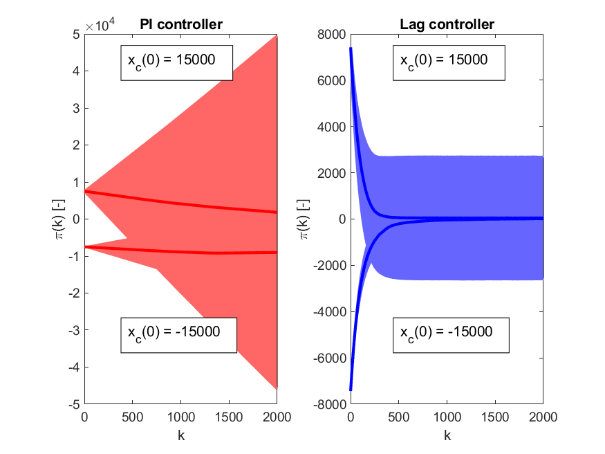
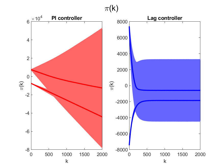
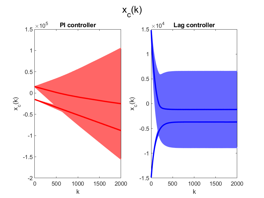
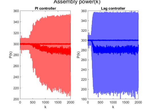
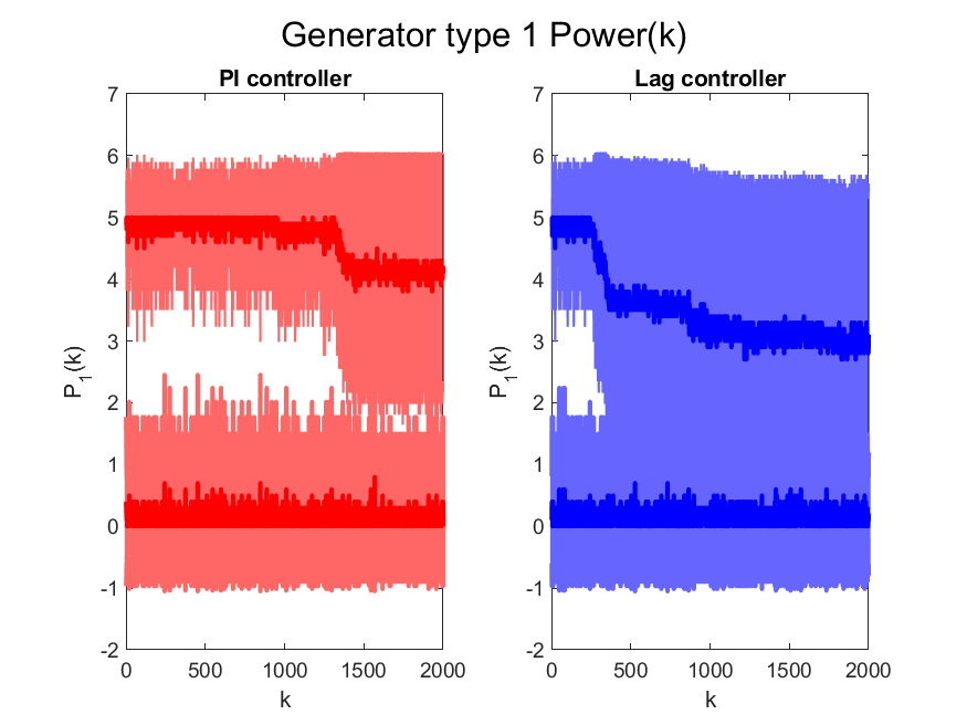
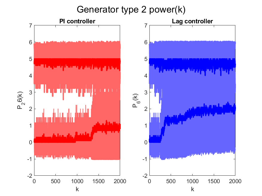
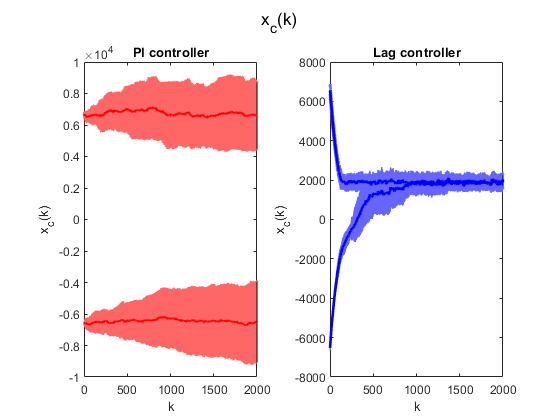
We repeated the simulations 300 times, considering the time horizon of 2000 time steps each. The results in Figures 3–5 present the mean over the 300 runs with a solid line and the region of mean standard deviation as a shaded area. Notice that we are able to regulate the aggregate power output (cf. Figure 3). With the PI controller, however, the state of the controller, and consequently the signal and the power generated at individual buses over the time horizon, are determined by the initial state of the controller (cf. Figures 4–5).
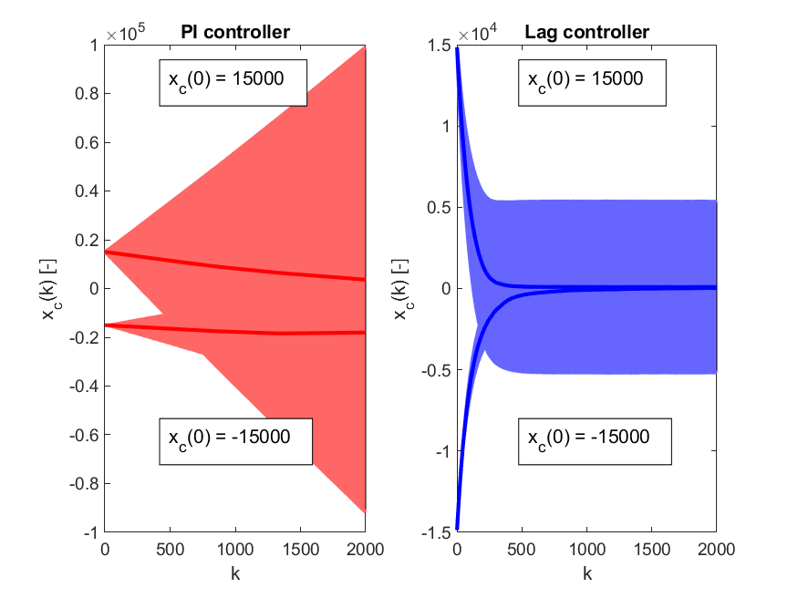
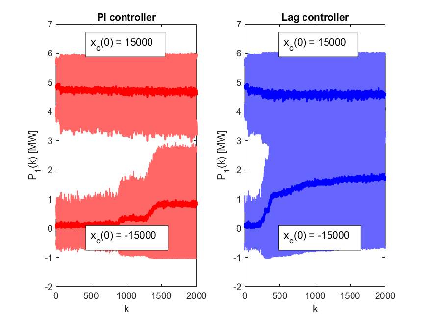
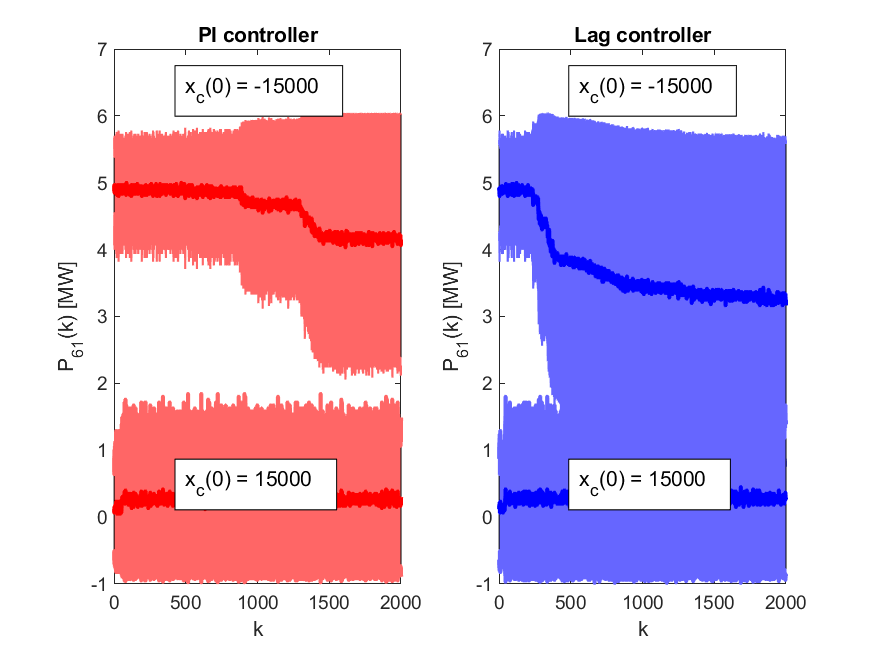
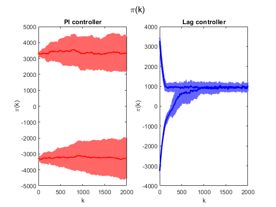
VI-B A Transmission-System Test Case
Next, let us demonstrate the analogous results on the standard IEEE 118-bus test case with minor modifications. Notably, the ensemble is connected to two buses of the transmission system. At bus 10, 1 generator with a maximum active power output of 450 MW was replaced by 8 DERs with 110 MW of power each, out of which 4 DERs used probability function , where . The other four DERs used function , where and . At bus 25, 1 generator with maximum active power output of 220 MW was replaced by four generators with active power output of 110 MW, out of which two generators used probability function , and the other two used function with .
As in the serial test case, we have repeated the simulations 500 times, considering the time horizon of 2000 time steps each. Figure 6 yields analogical results to Figure 4 in the serial test case, where a different initial state of the controller yields a very different control signal produced by the PI controller. This is not the case for the lag approximant. Consequently, some DERs may be activated much more often than others, all else being equal, solely as an artifact of the use of PI control. Many further simulation results illustrating this behaviour are available in the Supplementary material on-line.
VII Conclusions and Further Work
We have introduced a notion of predictability of fairness in load aggregation and demand-response management, which relies on the concept of unique ergodicity [83], which in turn is based on the existence of a unique invariant measure for a stochastic model of a closed-loop model of the system. Related notions of unique ergodicity have recently been used in social-sensing [83], and two-sided markets [84]; we envision it may have many further applications in power systems.
The notions of predictability and fairness, which we have introduced, may be violated, if controls with poles on the unit circle (e.g., PI) are applied to load aggregation. In particular, the application of the PI controller destroys the ergodicity of the closed-loop model. Considering the prevalence of PI controllers within load frequency control, this is a serious concern. On the other hand, we have demonstrated that certain other controllers guarantee predictability and fairness.
An important direction for further study is to consider unique ergodicity of stability-constrained ACOPF [28, 29, 30, 31, 32, 33, 34], or related controllers based on stability-constrained model-predictive control (MPC). We believe there are a wealth of important results ahead.
Acknowledgements
Ramen and Bob were supported in part by Science Foundation Ireland grant 16/IA/4610. Jakub has been supported by OP VVV project CZ.02.1.01/0.0/0.0/16_019/0000765 “Research Center for Informatics”.
References
- Lund et al. [2015] P. D. Lund, J. Lindgren, J. Mikkola, and J. Salpakari, “Review of energy system flexibility measures to enable high levels of variable renewable electricity,” Renewable and sustainable energy reviews, vol. 45, pp. 785–807, 2015.
- Conejo et al. [2010] A. Conejo, J. Morales, and L. Baringo, “Real-time demand response model,” IEEE Transactions on Smart Grid, vol. 1, no. 3, pp. 236–242, Dec. 2010.
- Callaway and Hiskens [2011] D. S. Callaway and I. A. Hiskens, “Achieving controllability of electric loads,” Proceedings of the IEEE, vol. 99, no. 1, pp. 184–199, Jan 2011.
- Pinson et al. [2014] P. Pinson, H. Madsen et al., “Benefits and challenges of electrical demand response: A critical review,” Renewable and Sustainable Energy Reviews, vol. 39, pp. 686–699, 2014.
- Mohsenian-Rad and Leon-Garcia [2010] A.-H. Mohsenian-Rad and A. Leon-Garcia, “Optimal residential load control with price prediction in real-time electricity pricing environments,” IEEE Transactions on Smart Grid, vol. 1, no. 2, pp. 120–133, Sep. 2010.
- Alagoz et al. [2013] B. B. Alagoz, A. Kaygusuz, M. Akcin, and S. Alagoz, “A closed-loop energy price controlling method for real-time energy balancing in a smart grid energy market,” Energy, vol. 59, pp. 95–104, 2013.
- Mathieu et al. [2014] J. L. Mathieu, M. Kamgarpour, J. Lygeros, G. Andersson, and D. S. Callaway, “Arbitraging intraday wholesale energy market prices with aggregations of thermostatic loads,” IEEE Transactions on Power Systems, vol. 30, no. 2, pp. 763–772, 2014.
- Shaukat et al. [2018] N. Shaukat, B. Khan, S. Ali, C. Mehmood, J. Khan, U. Farid, M. Majid, S. Anwar, M. Jawad, and Z. Ullah, “A survey on electric vehicle transportation within smart grid system,” Renewable and Sustainable Energy Reviews, vol. 81, pp. 1329–1349, 2018.
- Lee et al. [2020] Z. J. Lee, G. Lee, T. Lee, C. Jin, R. Lee, Z. Low, D. Chang, C. Ortega, and S. H. Low, “Adaptive charging networks: A framework for smart electric vehicle charging,” arXiv preprint arXiv:2012.02636, 2020.
- El Bakari and Kling [2010] K. El Bakari and W. L. Kling, “Virtual power plants: An answer to increasing distributed generation,” in 2010 IEEE PES Innovative Smart Grid Technologies Conference Europe (ISGT Europe). IEEE, 2010, pp. 1–6.
- Crisostomi et al. [2014] E. Crisostomi, M. Liu, M. Raugi, and R. Shorten, “Plug-and-play distributed algorithms for optimized power generation in a microgrid,” IEEE transactions on Smart grid, vol. 5, no. 4, pp. 2145–2154, 2014.
- Dall’Anese et al. [2018] E. Dall’Anese, S. S. Guggilam, A. Simonetto, Y. C. Chen, and S. V. Dhople, “Optimal regulation of virtual power plants,” IEEE Transactions on Power Systems, vol. 33, no. 2, pp. 1868–1881, 2018.
- Roozbehani et al. [2012] M. Roozbehani, M. A. Dahleh, and S. K. Mitter, “Volatility of power grids under real-time pricing,” IEEE Transactions on Power Systems, vol. 27, no. 4, pp. 1926–1940, Nov 2012.
- Li et al. [2020] T. Li, S. H. Low, and A. Wierman, “Real-time flexibility feedback for closed-loop aggregator and system operator coordination,” in Proceedings of the Eleventh ACM International Conference on Future Energy Systems, 2020, pp. 279–292.
- Baker [2021] K. Baker, “Solutions of dc opf are never ac feasible,” in Proceedings of the Twelfth ACM International Conference on Future Energy Systems, 2021, pp. 264–268.
- O’Neill-Carrillo et al. [1999] E. O’Neill-Carrillo, G. T. Heydt, E. J. Kostelich, S. S. Venkata, and A. Sundaram, “Nonlinear deterministic modeling of highly varying loads,” IEEE Transactions on Power Delivery, vol. 14, no. 2, pp. 537–542, Apr 1999.
- Rogers [2012] G. Rogers, Power system oscillations. Springer Science & Business Media, 2012.
- Fioravanti et al. [2019] A. R. Fioravanti, J. Mareček, R. N. Shorten, M. Souza, and F. R. Wirth, “On the ergodic control of ensembles,” Automatica, vol. 108, p. 108483, 2019.
- Zimmerman et al. [2010] R. D. Zimmerman, C. E. Murillo-Sánchez, and R. J. Thomas, “Matpower: Steady-state operations, planning, and analysis tools for power systems research and education,” IEEE Transactions on power systems, vol. 26, no. 1, pp. 12–19, 2010.
- Kundur et al. [1994] P. Kundur, N. J. Balu, and M. G. Lauby, Power system stability and control. McGraw-hill New York, 1994, vol. 7.
- Sauer and Pai [1998] P. W. Sauer and M. A. Pai, Power system dynamics and stability. Prentice hall Upper Saddle River, NJ, 1998, vol. 101.
- Machowski et al. [2011] J. Machowski, J. Bialek, and J. Bumby, Power system dynamics: stability and control. John Wiley & Sons, 2011.
- Bevrani [2014] H. Bevrani, Robust power system frequency control. Springer, 2014.
- Calovic [1972] M. Calovic, “Linear regulator design for a load and frequency control,” IEEE Transactions on Power Apparatus and Systems, vol. PAS-91, no. 6, pp. 2271–2285, Nov 1972.
- Pan and Liaw [1989] C. Pan and C. Liaw, “An adaptive controller for power system load-frequency control,” IEEE Transactions on Power Systems, vol. 4, no. 1, pp. 122–128, Feb 1989.
- Ugrinovskii and Pota [2005] V. Ugrinovskii and H. R. Pota, “Decentralized control of power systems via robust control of uncertain markov jump parameter systems,” International Journal of Control, vol. 78, no. 9, pp. 662–677, 2005.
- Perfumo et al. [2012] C. Perfumo, E. Kofman, J. H. Braslavsky, and J. K. Ward, “Load management: Model-based control of aggregate power for populations of thermostatically controlled loads,” Energy Conversion and Management, vol. 55, pp. 36 – 48, 2012.
- Zárate-Miñano et al. [2010] R. Zárate-Miñano, F. Milano, and A. J. Conejo, “An opf methodology to ensure small-signal stability,” IEEE Transactions on Power Systems, vol. 26, no. 3, pp. 1050–1061, 2010.
- Li et al. [2016] P. Li, J. Qi, J. Wang, H. Wei, X. Bai, and F. Qiu, “An sqp method combined with gradient sampling for small-signal stability constrained opf,” IEEE Transactions on Power Systems, vol. 32, no. 3, pp. 2372–2381, 2016.
- Wang et al. [2018] C. Wang, B. Cui, Z. Wang, and C. Gu, “Sdp-based optimal power flow with steady-state voltage stability constraints,” IEEE Transactions on Smart Grid, vol. 10, no. 4, pp. 4637–4647, 2018.
- Li et al. [2019] Y. Li, G. Geng, Q. Jiang, W. Li, and X. Shi, “A sequential approach for small signal stability enhancement with optimizing generation cost,” IEEE Transactions on Power Systems, vol. 34, no. 6, pp. 4828–4836, 2019.
- Nojavan and Seyedi [2020] M. Nojavan and H. Seyedi, “Voltage stability constrained opf in multi-micro-grid considering demand response programs,” IEEE Systems Journal, vol. 14, no. 4, pp. 5221–5228, 2020.
- Nikkhah et al. [2020] S. Nikkhah, M.-A. Nasr, and A. Rabiee, “A stochastic voltage stability constrained ems for isolated microgrids in the presence of pevs using a coordinated uc-opf framework,” IEEE Transactions on Industrial Electronics, vol. 68, no. 5, pp. 4046–4055, 2020.
- Pullaguram et al. [2021] D. Pullaguram, R. Madani, T. Altun, and A. Davoudi, “Small signal stability constrained optimal power flow for inverter dominant autonomous microgrids,” IEEE Transactions on Industrial Electronics, pp. 1–1, 2021.
- Heydt [1983] G. T. Heydt, “The impact of electric vehicle deployment on load management straregies,” IEEE Transactions on Power Apparatus and Systems, vol. PAS-102, no. 5, pp. 1253–1259, May 1983.
- Infield et al. [2007] D. G. Infield, J. Short, C. Horne, and L. L. Freris, “Potential for domestic dynamic demand-side management in the uk,” in 2007 IEEE Power Engineering Society General Meeting, June 2007, pp. 1–6.
- Xu et al. [2011] Z. Xu, J. Ostergaard, and M. Togeby, “Demand as frequency controlled reserve,” IEEE Transactions on Power Systems, vol. 26, no. 3, pp. 1062–1071, Aug 2011.
- Douglass et al. [2013] P. J. Douglass, R. Garcia-Valle, P. Nyeng, J. Østergaard, and M. Togeby, “Smart demand for frequency regulation: Experimental results,” IEEE Transactions on Smart Grid, vol. 4, no. 3, pp. 1713–1720, Sep. 2013.
- Biegel et al. [2014] B. Biegel, L. H. Hansen, J. Stoustrup, P. Andersen, and S. Harbo, “Value of flexible consumption in the electricity markets,” Energy, vol. 66, pp. 354 – 362, 2014.
- Angeli and Kountouriotis [2012] D. Angeli and P. Kountouriotis, “A stochastic approach to “dynamic-demand” refrigerator control,” IEEE Transactions on Control Systems Technology, vol. 20, no. 3, pp. 581–592, May 2012.
- Samarakoon et al. [2012] K. Samarakoon, J. Ekanayake, and N. Jenkins, “Investigation of domestic load control to provide primary frequency response using smart meters,” IEEE Transactions on Smart Grid, vol. 3, no. 1, pp. 282–292, March 2012.
- Bashash and Fathy [2013] S. Bashash and H. K. Fathy, “Modeling and control of aggregate air conditioning loads for robust renewable power management,” IEEE Transactions on Control Systems Technology, vol. 21, no. 4, pp. 1318–1327, July 2013.
- Pourmousavi and Nehrir [2012] S. A. Pourmousavi and M. H. Nehrir, “Real-time central demand response for primary frequency regulation in microgrids,” IEEE Transactions on Smart Grid, vol. 3, no. 4, pp. 1988–1996, Dec 2012.
- Subramanian et al. [2012] A. Subramanian, M. Garcia, A. Domínguez-García, D. Callaway, K. Poolla, and P. Varaiya, “Real-time scheduling of deferrable electric loads,” in 2012 American Control Conference (ACC), June 2012, pp. 3643–3650.
- Mu et al. [2013] Y. Mu, J. Wu, J. Ekanayake, N. Jenkins, and H. Jia, “Primary frequency response from electric vehicles in the great britain power system,” IEEE Transactions on Smart Grid, vol. 4, no. 2, pp. 1142–1150, June 2013.
- Biegel et al. [2013] B. Biegel, L. H. Hansen, P. Andersen, and J. Stoustrup, “Primary control by on/off demand-side devices,” IEEE Transactions on Smart Grid, vol. 4, no. 4, pp. 2061–2071, Dec 2013.
- Gouveia et al. [2013] C. Gouveia, J. Moreira, C. L. Moreira, and J. A. Peças Lopes, “Coordinating storage and demand response for microgrid emergency operation,” IEEE Transactions on Smart Grid, vol. 4, no. 4, pp. 1898–1908, Dec 2013.
- Zhao et al. [2014] C. Zhao, U. Topcu, N. Li, and S. Low, “Design and stability of load-side primary frequency control in power systems,” IEEE Transactions on Automatic Control, vol. 59, no. 5, pp. 1177–1189, May 2014.
- Pourmousavi and Nehrir [2014] S. A. Pourmousavi and M. H. Nehrir, “Introducing dynamic demand response in the lfc model,” IEEE Transactions on Power Systems, vol. 29, no. 4, pp. 1562–1572, July 2014.
- Weckx et al. [2015] S. Weckx, R. D’Hulst, and J. Driesen, “Primary and secondary frequency support by a multi-agent demand control system,” IEEE Transactions on Power Systems, vol. 30, no. 3, pp. 1394–1404, May 2015.
- Hao et al. [2014] H. Hao, Y. Lin, A. S. Kowli, P. Barooah, and S. Meyn, “Ancillary service to the grid through control of fans in commercial building hvac systems,” IEEE Transactions on Smart Grid, vol. 5, no. 4, pp. 2066–2074, July 2014.
- Dörfler and Grammatico [2017] F. Dörfler and S. Grammatico, “Gather-and-broadcast frequency control in power systems,” Automatica, vol. 79, pp. 296–305, 2017.
- Tindemans et al. [2015] S. H. Tindemans, V. Trovato, and G. Strbac, “Decentralized control of thermostatic loads for flexible demand response,” IEEE Transactions on Control Systems Technology, vol. 23, no. 5, pp. 1685–1700, Sep. 2015.
- Ersdal et al. [2016] A. M. Ersdal, L. Imsland, and K. Uhlen, “Model predictive load-frequency control,” IEEE Transactions on Power Systems, vol. 31, no. 1, pp. 777–785, Jan 2016.
- Mallada et al. [2017] E. Mallada, C. Zhao, and S. Low, “Optimal load-side control for frequency regulation in smart grids,” IEEE Transactions on Automatic Control, vol. 62, no. 12, pp. 6294–6309, Dec 2017.
- Dehghanpour and Afsharnia [2015] K. Dehghanpour and S. Afsharnia, “Electrical demand side contribution to frequency control in power systems: a review on technical aspects,” Renewable and Sustainable Energy Reviews, vol. 41, pp. 1267 – 1276, 2015.
- Elton [1987a] J. H. Elton, “An ergodic theorem for iterated maps,” Ergodic Theory and Dynamical Systems, vol. 7, no. 04, pp. 481–488, 1987.
- Barnsley et al. [1988a] M. Barnsley, S. Demko, J. Elton, and J. Geronimo, “Invariant measures for Markov processes arising from iterated function systems with place-dependent probabilities,” Annales de l’institut Henri Poincaré (B) Probabilités et Statistiques, vol. 24, no. 3, pp. 367–394, 1988.
- Barnsley et al. [1989a] M. F. Barnsley, J. H. Elton, and D. P. Hardin, “Recurrent iterated function systems,” Constructive approximation, vol. 5, no. 1, pp. 3–31, 1989.
- Elton [1987b] J. H. Elton, “An ergodic theorem for iterated maps,” Ergodic Theory and Dynamical Systems, vol. 7, no. 04, pp. 481–488, 1987.
- Barnsley and Elton [1988] M. F. Barnsley and J. H. Elton, “A new class of markov processes for image encoding,” Advances in applied probability, vol. 20, no. 1, pp. 14–32, 1988.
- Barnsley et al. [1989b] M. F. Barnsley, J. H. Elton, and D. P. Hardin, “Recurrent iterated function systems,” Constructive approximation, vol. 5, no. 1, pp. 3–31, 1989.
- Kifer [2012] Y. Kifer, Ergodic theory of random transformations. Springer Science & Business Media, 2012, vol. 10.
- Bhattacharya and Waymire [2009] R. N. Bhattacharya and E. C. Waymire, Stochastic processes with applications. SIAM, 2009.
- Stenflo [1999] Ö. Stenflo, “Ergodic theorems for iterated function systems controlled by stochastic sequences,” PhD thesis, 1999.
- Barnsley et al. [1988b] M. F. Barnsley, S. G. Demko, J. H. Elton, and J. S. Geronimo, “Invariant measures for markov processes arising from iterated function systems with place-dependent probabilities,” in Annales de l’IHP Probabilités et statistiques, vol. 24, 1988, pp. 367–394.
- Barnsley [2013] M. Barnsley, Fractals Everywhere, ser. Dover books on mathematics. Dover Publications, 2013.
- Stenflo [2001] Ö. Stenflo, “Markov chains in random environments and random iterated function systems,” Transactions of the American Mathematical Society, vol. 353, no. 9, pp. 3547–3562, 2001.
- Szarek [2003] T. Szarek, “Invariant measures for markov operators with application to function systems,” Studia Mathematica, vol. 154, pp. 207–222, 01 2003.
- Steinsaltz [1999] D. Steinsaltz, “Locally contractive iterated function systems,” Annals of Probability, vol. 27, no. 4, pp. 1952–1979, 1999.
- Walkden [2007] C. P. Walkden, “Invariance principles for interated maps that contract on average,” Transactions of the American Mathematical Society, vol. 359, no. 3, pp. 1081–1097, 2007. [Online]. Available: http://www.jstor.org/stable/20161616
- Bárány [2015] B. Bárány, “On iterated function systems with place-dependent probabilities,” Proc. Amer. Math. Soc., vol. 143, pp. 419–432, 2015.
- Diaconis and Freedman [1999] P. Diaconis and D. Freedman, “Iterated random functions,” SIAM Review, vol. 41, no. 1, pp. 45–76, 1999.
- Iosifescu [2009] M. Iosifescu, “Iterated function systems: A critical survey,” Math. Reports, vol. 11, no. 3, pp. 181–229, 2009.
- Stenflo [2012] Ö. Stenflo, “A survey of average contractive iterated function systems,” Journal of Difference Equations and Applications, vol. 18, no. 8, pp. 1355–1380, 2012.
- Franklin et al. [1994] G. F. Franklin, J. D. Powell, and A. B. Emami-Naeini, Feedback Control of Dynamic Systems. Reading, MA: Addison Wesley, 1994.
- Franklin et al. [1997] G. F. Franklin, J. D. Powell, and M. L. Workman, Digital Control of Dynamic Systems, 3rd ed. Englewood Cliffs, NJ: Prentice Hall, 1997.
- Barker and Cronin [2007] W. Barker and M. Cronin, “Speedtronic™ mark vi turbine control system,” Ge Power Systems Ger, Schenectady, NY, Report No. GER-4193A, 2007.
- Angeli [2002] D. Angeli, “A Lyapunov approach to incremental stability properties,” IEEE Transactions on Automatic Control, vol. 47, no. 3, pp. 410–421, 2002.
- Tran et al. [2018] D. N. Tran, B. S. Rüffer, and C. M. Kellett, “Convergence properties for discrete-time nonlinear systems,” IEEE Transactions on Automatic Control, vol. 64, no. 8, pp. 3415–3422, 2018.
- Jiang and Wang [2002] Z.-P. Jiang and Y. Wang, “A converse Lyapunov theorem for discrete-time systems with disturbances,” Systems & control letters, vol. 45, no. 1, pp. 49–58, 2002.
- Marruedo et al. [2002] D. L. Marruedo, T. Alamo, and E. F. Camacho, “Input-to-state stable mpc for constrained discrete-time nonlinear systems with bounded additive uncertainties,” in Proceedings of the 41st IEEE Conference on Decision and Control, 2002., vol. 4, Dec 2002, pp. 4619–4624 vol.4.
- Ghosh et al. [2021a] R. Ghosh, J. Mareček, W. M. Griggs, M. Souza, and R. N. Shorten, “Predictability and fairness in social sensing,” IEEE Internet of Things Journal, pp. 1–1, 2021.
- Ghosh et al. [2021b] R. Ghosh, W. M. Griggs, J. Marecek, and R. N. Shorten, “Unique ergodicity in the interconnections of ensembles with applications to two-sided markets,” 2021.
For the convenience of the reader, we attach an overview of the notation and additional numerical results in the following appendices.
-A An Overview of Notation
|
|
||
|---|---|---|
| \endfirsthead \endhead continues on next page | ||
| \endfoot \endlastfootSymbol | Meaning | |
| the set of natural numbers. | ||
| the set of rational numbers. | ||
| the set of real numbers. | ||
| states-space of agent . | ||
| states-space of controller. | ||
| states-space of filter. | ||
| overall states-space of the closed loop system. | ||
| set of all integers. | ||
| an event i.e an element in . | ||
| an index set. | ||
| a closed subset of . | ||
| A Borel algebra on , consisting of all possible events. | ||
| A discrete-time Markov chain with state-space . | ||
| A transition-probability operator. | ||
| the probability measure induced on the path space. | ||
| probability measures. | ||
| a probability measure. | ||
| an element in . | ||
| cardinality of output maps. | ||
| a function on . | ||
| probability functions. | ||
| control signal. | ||
| space of all control signal. | ||
| space of all agent’s actions. | ||
| possibles actions. | ||
| cardinality of action space of agent . | ||
| demand space of agent . | ||
| possible demands. | ||
| cardinality of demand space of agent . | ||
| dimension of the state-space of agent’s private state-space. | ||
| an affine map. | ||
| number of output maps. | ||
| output maps. | ||
| output of agent . | ||
| value of filtered by filter. | ||
| probability functions. | ||
| probability functions. | ||
| internal state of agent at time . | ||
| transition maps. | ||
| a filter. | ||
| a controller. | ||
| the internal state of the filter at time of dimension . | ||
| the internal state of the filter at time of dimension | ||
| map moddeling the controller. | ||
| map moddeling the controller | ||
| a sufiiciently small positive real number | ||
| Lipschitz constants. | ||
| an invariant distribution. | ||
| a class function. | ||
| a class function. | ||
| a binary vector indicating the commitment of DERs in (30). | ||
| filtered value of the active power output of DERs in (32). | ||
| active power output of DERs in (31). | ||
| aggregate active power output of the ensemble at time . | ||
| error defined in (33). | ||
-B Complete Numerical Results
We provide numerical results for three test cases, two of which have been discussed in the main body of the text. First, however, we present results for one additional, intentionally simple test case.
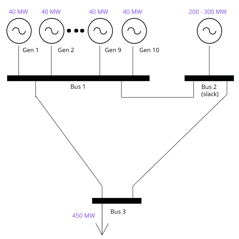
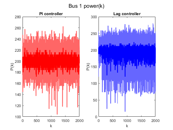
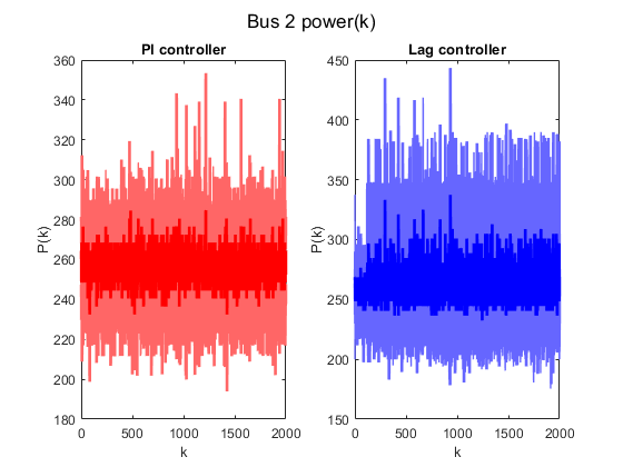
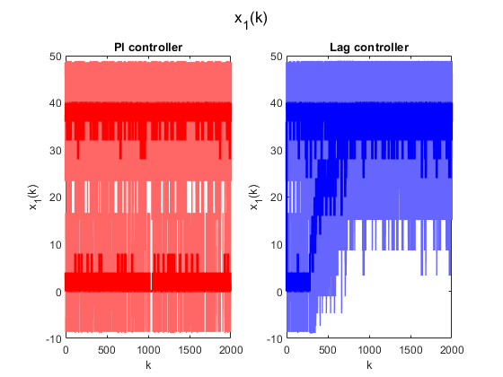
-B1 A Simple Test Case with Transmission Losses in the Filter
The first one is a small 3-bus system depicted in Figure 1. At bus 1, there are DERs, five of which use probability function with . The other five DERs at bus 1 use function , where and . Bus 2 is considered slack; therefore, the generator at bus 2 balances the power deviation of bus 1 and losses in order to fulfil power demand at bus 3. The simulations were run for both PI and its lag approximant for several different initial values of the controller’s internal state . Figures 9–LABEL:fig:sim1sig demonstrate that both controllers can regulate the ensemble around required power . However, the PI controller’s behaviour is strongly dependent on the initial condition of its internal state, whereas the lag approximant provides predictable behaviour in the long run. These results are in good agreement with simulation results in [18].
-C A Serial Test Case with Losses in the Filter
In our second example, we consider a serial test-case, with a number of buses connected in series. (A line-graph topology, in the language of graph theory.) The buses are, in this order,
-
•
a slack bus, which could represent a distribution substation
-
•
5 buses with 12 DERs of 5 MW capacity each, and the “type 2” probability function.
-
•
5 buses with 12 DERs of 5 MW capacity each, and the “type 1” probability function.
-
•
a single load bus with a 500 MW demand.
Overall, the ensemble is composed of 120 DERs, with a total capacity of 600 MW. Initially, the first generators are off and the second following generators are on. We aim to regulate the power output of the ensemble to 60 running DERs (totalling 300 MW), which should yield a load exceeding 200 MW on the slack bus (considering the losses).
In our first set of simulations on the serial test case, we repeat 500 times the simulations considering the time horizon of 2000 time steps each. , . The filter is , whereby the losses hence propagate into the signal .
As in the simple test case, we are able to regulate the aggregate power output (cf. Figure 13). With PI controller, however, the state of the controller, and consequently the signal and the power at individual buses are determined by the initial state of the controller (cf. Figures 14–15).

In our second set of simulations on the serial test case, we repeat 500 times the simulations considering the time horizon of 2000 time steps each. Instead of , of the first set of simulations, we consider to be plus losses at time , and similarly to be plus losses at time . Otherwise, the system’s behaviour is similar.
As above, we are able to regulate the aggregate power output (cf. Figure 16). With PI controller, however, the state of the controller, and consequently the signal and the power at individual buses are determined by the initial state of the controller (cf. Figures 17–18).
-D A Transmission-System Test Case with Losses in the Filter
The third example demonstrates the procedure’s applicability to the standard IEEE 118-bus test case with minor modifications. Notably, the ensemble is connected to two buses of the transmission system. At bus 10, 1 generator with a maximum active power output of 450 MW was replaced by 8 DERs with 110 MW of power each, out of which 4 DERs used probability function , where . The other four DERs used function , where and . At bus 25, 1 generator with maximum active power output of 220 MW was replaced by four generators with active power output of 110 MW, out of which two generators used probability function , and the other two used function with . Bus 69 is the slack bus, similarly to the generator at bus 3 in the previous example. Figures -D–-D yield analogical results to the first example, for both controllers and different initial conditions .
![[Uncaptioned image]](/html/2110.03001/assets/case118_pf_01/118_01_bus_10_power.png)
![[Uncaptioned image]](/html/2110.03001/assets/case118_pf_01/118_03_gen_1_power.png)
![[Uncaptioned image]](/html/2110.03001/assets/case118_pf_01/118_05_gen_9_power.png)
![[Uncaptioned image]](/html/2110.03001/assets/case118_pf_01/118_06_gen_11_power.png)