NUS-IDS at FinCausal 2021: Dependency Tree in Graph Neural Network for Better Cause-Effect Span Detection

Abstract

Automatic identification of cause-effect spans in financial documents is important for causality modelling and understanding reasons that lead to financial events. To exploit the observation that words are more connected to other words with the same cause-effect type in a dependency tree, we construct useful graph embeddings by incorporating dependency relation features through a graph neural network. Our model builds on a baseline BERT token classifier with Viterbi decoding, and outperforms this baseline in cross-validation and during the competition. In the official run of FinCausal 2021, we obtained Precision, Recall, and F1 scores of $95.56\%$, $95.56\%$ and $95.57\%$ that all ranked 1^st place, and an Exact Match score of $86.05\%$ which ranked 3^rd place.

1 Introduction

We worked on the shared task of FinCausal 2021 (Mariko et al., 2021) that aims to identify cause and effect spans in financial news. This task builds on the previous shared Task 2 (Mariko et al., 2020) by introducing additional annotated data.

Contributions:

We propose a solution to include dependency relations in a sentence to improve identification of cause-effect spans. We do so by representing dependency relations in a graph neural network. Our model is an extension of a baseline BERT token classifier with Viterbi decoding (Kao et al., 2020), and outperforms this baseline in cross-validation and test settings. This improvement also holds for two BERT pretrained language models that were experimented with. During the competition, we ranked 1^st for Precision, Recall, and F1 scores and 3^rd for Exact Match score.

Organization:

Section 2 outlines our approach for this task. Section 3 introduces the task dataset and evaluation datasets. Our results are presented and discussed in Section 4 while Section 5 concludes with some future directions.

2 Our Approach

In this section, we outline our approach . Additional architectural and experimental details are provided in the Appendix.

2.1 Framing the Task

Given an example document, which could be one or multiple sentence(s) long, the task is to identify the cause and effect substrings. We converted the span detection task into a token classification task, similar to many state-of-the-art methodologies for span detection (Pavlopoulos et al., 2021) and Named Entity Recognition (Lample et al., 2016; Tan et al., 2020) tasks. Figure 1 demonstrates an example sentence that has its Cause (C) span highlighted in green, and Effect (E) span highlighted in orange, while all other spans are highlighted in grey. The sentence was tokenized and subsequently aligned against the target token labels. We included the BIO format (Begin, Inside, Outside) (Ramshaw and Marcus, 1995) in our labels to better identify the start of spans. Thus, we have five labels: B-C, I-C, B-E, I-E and O.

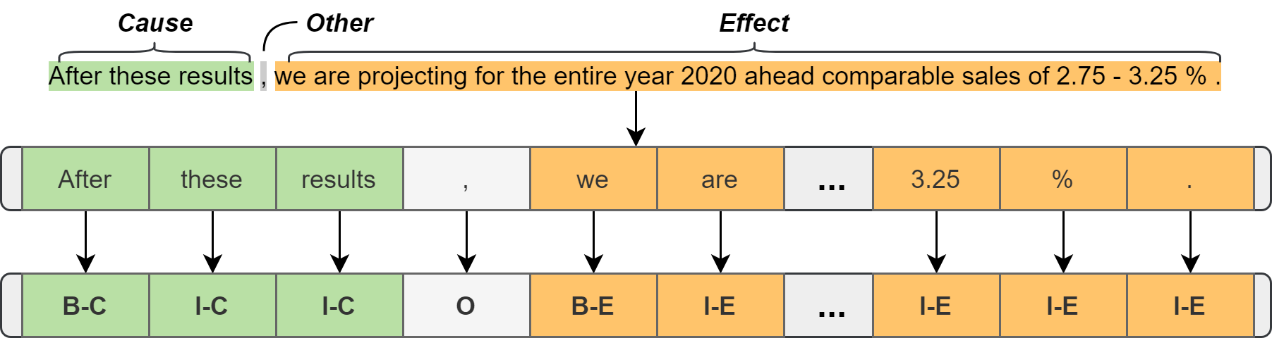
Figure 1: Illustrative training example (ID: 0477.00020) with Cause (C) and Effect (E) spans highlighted in green and orange respectively. We include Begin (B), Inside (I) and Outside (O) prefixes to create 5 labels in our token classification task.

2.2 Baseline

Kao et al. demonstrated that their BIO tagging scheme with a Viterbi decoder (Viterbi, 1967) that utilised BERT-encoded document representations is useful for this cause-effect span detection task. Their model topped the competition last year across all metrics. Therefore, we adapted their pipeline and proposed distinct additions highlighted later in Section 2.3 for improved performance. In the immediate subsections, we motivate the benefits in retaining the key components of Kao et al.’s model, and highlight any differences in our approach.

2.2.1 BERT Embeddings

We employed the Bidirectional Encoder Representations from Transformers (BERT) (Devlin et al., 2019) for its tokenizer and encoder model, fine-tuned on our task. We used pretrained language models from Huggingface (Wolf et al., 2020). Apart from bert-base-cased, we also used bert-large-cased for improved performance.

2.2.2 Viterbi Decoder

The Viterbi decoding algorithm is only applied during evaluation. Since the true cause-effect spans are consecutive sequences, but the token classifications from the neural network could produce non-consecutive sequences, the Viterbi algorithm serves as a forward error correction technique and is an important element for the success of this pipeline.

2.2.3 Parts-of-Speech

Kao et al. (2020) showed that Parts-of-Speech (POS) did not improve their model performance. We reconfirm this finding later in Section 4.2. However, we found POS features to be useful inclusions for our proposed model.

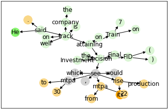
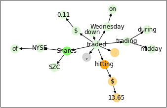
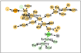
Figure 2: Dependency-tree represented as directed graphs, with Cause, Effect, and Other spans highlighted in green, orange and grey respectively.

2.3 Dependency Tree

Our key contribution is the inclusion of dependency tree relations into the neural network for improved cause-effect token classification. Dependencies in text can be mapped into a directed graph representation, where nodes represent words and edges represent the dependency relation. Figure 2 shows some example sentences, highlighted by their Cause and Effect labels. We notice that there is a tendency for words of the same cause-effect label to be more connected in these graphs and thus wish to incorporate these information into the model as features.

Figure 3 reflects our neural network model, with the addition of our GNN module that produces graph representations, which are then concatenated with the BERT and POS embeddings and fed into a linear layer for token classification. The following subsections describe the GNN module further.

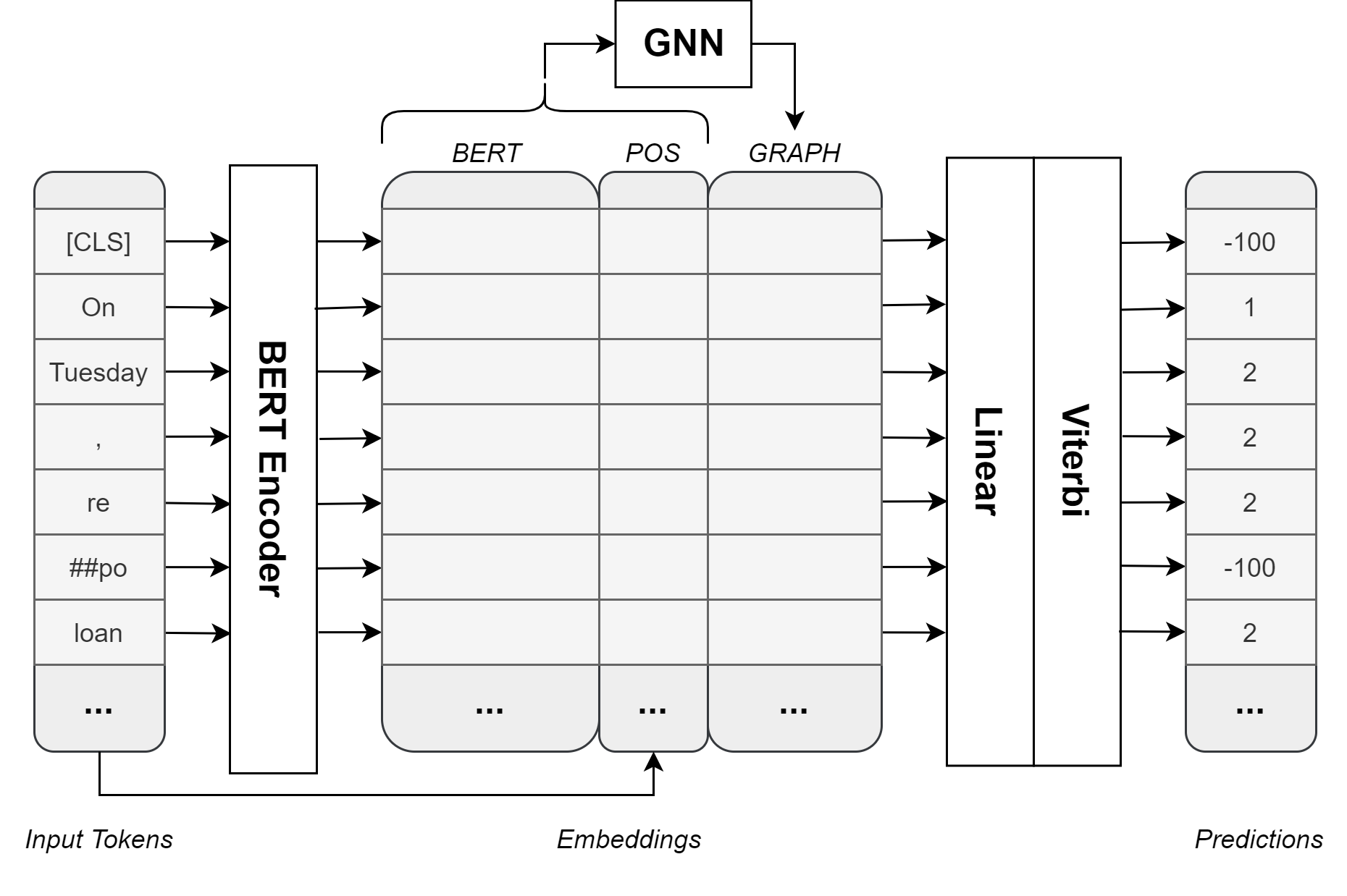
Figure 3: Neural network pipeline. Appendix A.1 outlines this further.

Model			Precision	Recall	F1	ExactMatch
A. bert-base-cased
1	Baseline		95.62	95.90	95.76	88.18
2	+ Node features, BiLSTM		95.42	95.95	95.68	88.07
3	Baseline w/ POS		95.39^	96.02	95.70	88.24
4	+ Node features		95.66	95.81	95.73	88.20
5	+ BiLSTM		95.46	95.99	95.72	88.06
6	+ Node features, BiLSTM (Proposed)		95.73	96.05^	95.89	88.35
B. bert-large-cased
7	Baseline		95.64	96.01	95.82	87.65
8	+ Node features, BiLSTM		93.75*	95.56	94.61*	86.44
9	Baseline w/ POS		94.46	96.08	95.22	87.28
10	+ Node features		95.61	95.98	95.79	88.24
11	+ BiLSTM		95.60	95.78^	95.69	87.94
12	+ Node features, BiLSTM (Proposed)		95.72	96.11	95.91	88.35

Table 1: Average evaluation results over cross-validation sets from 5 random seeds, each with 3 folds. Notes. Scores are reported in percentages (%). Best score per Panel per column is bolded. Baseline models are our replications of the models introduced by Kao et al. (2020). For each Panel A and B, Paired T-test of the models was conducted against Row 1 and 7 respectively, with statistical significance indicated by: ***$<0.05$, **$<0.10$, *$<0.15$, ^$<0.20$.

Model		Precision		Recall		F1		ExactMatch
Baseline		93.47		93.42		93.65		80.25
Proposed (bert-base-cased)		94.24		94.21		94.37		83.23
Proposed (bert-large-cased)		95.56		95.56		95.57		86.05
Best Score		95.56		95.56		95.57		87.77
Our Ranking		1st		1st		1st		3rd

Table 2: Results over test sets submitted to Codalab (As of 01 September 2021). Notes. Scores are reported in percentages (%). Best score per column is bolded. The models of the first three rows corresponds to Rows 1, 6, and 12 in Table 1 for CV respectively.

2.3.1 Document to Graph

Each example was represented as a directed graph, where nodes are token features (the concatenation of BERT and POS embeddings), while edges are directed connections pointing head to tail tokens based on dependency tree parsing .

2.3.2 Graph Neural Network

Our graph neural network (GNN) comprised of two graph convolutional layers for message passing across dependency relations that are two steps apart. Specifically, we used SAGEConv operator (Hamilton et al., 2017) for its ability to include node features and generate embeddings by aggregating a node’s neighbouring information. To capture the long-term contextual dependencies in both forward and backwards order of the original sentence, we added a bi-directional long short-term memory (BiLSTM) layer (Hochreiter and Schmidhuber, 1997) onto the graph embeddings.

3 Data

3.1 Task Dataset

Our main dataset is the FinCausal 2021 dataset (Mariko et al., 2021) comprising of $2393$ train and $638$ competition test examples.

3.2 Evaluation

We evaluated our proposed models in cross-validation (CV) against the Viterbi BERT model (Kao et al., 2020) that achieved first place in the previous run of this shared task. We refer to this model as the Baseline in subsequent sections. To check if our proposed models has statistically significant improvements from the Baseline, we adapted Dietterich (1998)’s approach using a 3-fold CV setup for 5 iterations, each iteration initialised with a random seed . This gives us $5*3=15$ sets of evaluation results to perform Paired T-Tests for statistical significance.

To obtain test predictions for submission on Codalab , we used a new $seed=123$ to train on the full train data and applied the model onto the unseen competition test data for online submission.

4 Results and Analysis

Table 1 reflects the model performances in CV, while Table 2 reflects the results during the competition. In both cases, we demonstrate that our model (Proposed) surpasses the Baseline.

For the CV setting, Proposed (Row 6) obtained $95.73\%$ Precision (P), $96.05\%$ Recall (R), $95.89\%$ F1 and $88.35\%$ exact match (EM) scores. These exceed the Baseline (Row 1) by $0.11\%$, $0.15\%$, $0.13\%$ and $0.18\%$ respectively . For test setting, large performance increments were observed: Proposed achieved P/R/F1/EM scores of $94.24\%$, $94.21\%$, $94.37\%$ and $83.23\%$, which are improvements from Baseline by a magnitude of $0.77\%$, $0.78\%$, $0.72\%$ and $2.98\%$ respectively .

4.1 Size of Pretrained Models

The two sections of Table 1 shows that the inclusion of dependency-based graph embeddings improved performance against Baseline irregardless of the pretrained BERT model choice.

Between the two investigated BERT models, bert-large-cased outperforms bert-base-cased by a small amount in CV and by a significant amount in testing across metrics. With bert-large-cased, the Proposed model achieved P/R/F1/EM scores of $95.56\%$, $95.56\%$, $95.57\%$ and $86.05\%$ during the competition, which are improvements from Baseline by a magnitude of $2.09\%$, $2.14\%$, $1.92\%$ and $5.80\%$ respectively .

4.2 Features and Layers

Table 1 also includes results from CV experiments where we removed components of our model. In this subsection, we discuss the importance of each component in the context of bert-base-cased, but note that similar findings persisted in the bert-large-cased.

POS:

Inclusion of the POS into the Baseline led to mixed outcomes across the four metrics against the Baseline (Row 3 vs Row 1). However, adding POS features in Proposed improved performance in all metrics (Row 6 vs Row 2).

Node features:

We reran a model that takes in nodes with no features (i.e. all nodes are represented by “$1$”). The results from this model corresponds to Row 5. No obvious improvements from Baseline (Row 1) was found, however, the performance was consistently worse off than Proposed for all metrics (Row 6), suggesting that informative node features are important to include in the GNN.

BiLSTM:

Comparing our proposed model with (Row 6) and without (Row 4) the BiLSTM layer suggested the layer was an important addition. Our hypothesis is that the BiLSTM helps to align the graph embeddings into a sequential manner corresponding to the original token order. A simple example is the punctuation full-stop “.” in Figure 2. The target label of the full-stop in these cases coincides with the immediate label of the word before it. However, our dependency tree attributed the full-stop as a tail of another word far away from it in the sentence (E.g. “said” $\rightarrow$ “.”).

5 Conclusions and Future Work

We have demonstrated the benefits of including dependency tree features as graph embeddings in a neural network model for better cause-effect span detection. A key caveat of our approach, which requires further research, is that dependency parsing occurs within sentences, resulting in disconnected graphs for examples with multiple sentences . Another future work is to apply our cause-effect detection model trained on financial texts onto other domains (E.g. academic journals) to study its generalizability.

Appendix A Appendix

A.1 Architecture of Proposed Model

An example with $n$ tokens can be represented by the vector of tokens $\underline{w}=(w_{0},w_{1},...,w_{n})^{\mathsf{T}}$, where $w$ refers to a BERT input token. A single token in this vector is represented by $w_{i}$, where $i$ denotes the location index of the token within the example. The tokenized example also has a matrix of POS features $V=(\underline{v_{0}},\underline{v_{1}},...,\underline{v_{n}})^{\mathsf{T}}$, where each $\underline{v_{i}}\in{\rm I\!R}^{d_{POS}}$ refers to a one-hot encoding across all POS tags, and so $d_{POS}$ reflects the number of possible POS tags.

To obtain BERT representations ($r$), we run the tokenized sequence vector through the BERT encoder ($T$) to obtain $r$ for each token $i$. Thus, we have that,

$$\underline{{r}_{i}}=T_{w}(\underline{w})_{i}, \underline{{r}_{i}}\in{\rm I\!R}^{d_{BERT}}$$ (1)

where $d_{BERT}$ refers to the output dimension for BERT encoder.

A dropout layer is represented by $\delta\sim Bernoulli(\rho)$, where $\rho$ refers to the dropout probability. We apply the dropout layer onto the BERT representations as follows,

$$\tilde{\underline{{r}_{i}}}=\delta*\underline{{r}_{i}}, {r}_{i}\in{\rm I\!R}^{d_{BERT}}$$ (2)

We combine the BERT and POS representations of each token together by a simple concatenation along the feature dimension.

$$\underline{{r_{2}}_{i}}=[\tilde{\underline{{r}_{i}}},\underline{v_{i}}], \underline{{r_{2}}_{i}}\in{\rm I\!R}^{d_{BERT}+d_{POS}}$$ (3)

Our GNN model generates graph embedding based on these concatenated features, which are then concatenated together to arrive at our final embeddings.

$$\underline{{r_{3}}_{i}}=GNN(\underline{{r_{2}}_{i}}), \underline{{r_{3}}_{i}}\in{\rm I\!R}^{d_{GNN}}$$ (4)

$$\underline{{r_{4}}_{i}}=[\underline{{r_{2}}_{i}},\underline{{r_{3}}_{i}}], \underline{{r_{4}}_{i}}\in{\rm I\!R}^{d}$$ (5)

$d_{GNN}$ refers to the output dimension for the last layer in our GNN module introduced in Section 2.3. That is, if BiLSTM is opted, then $d_{GNN}$ refers to the size of the output dimension of the BiLSTM layer. If not, it refers to the output dimension for the second SAGEConv layer. Our final representations have a feature dimension size of $d=d_{BERT}+d_{POS}+d_{GNN}$.

Next, we run our combined embeddings through a linear layer to obtain predicted probabilities per token. $c$ refers to the number of classes to be predicted.

$$\underline{{o}_{i}}=\underline{{r_{4}}_{i}}*W+\underline{b_{i}},$$

$$W\in{\rm I\!R}^{d\times c}, \underline{{o}_{i}},\underline{{b}_{i}}\in{\rm I\!R}^{c}$$ (6)

Cross entropy loss was used during training to optimize model weights. In evaluation, the logits ran through a Viterbi decoder for adjustment. Finally, all logits ran through an argmax function to obtain the predicted class that had the highest probability.

In our implementation, we set $d_{BERT}=768$, $d_{POS}=51$, $d_{GNN}=512$ and $c=5$.

A.2 Replication Checklist

• Hyperparameters: Our pretrained BERT models were initialized with the default configuration from Huggingface (Wolf et al., 2020). To train our model, we used the Adam optimizer with $\beta 1=0.9$, $\beta 2=0.999$. Learning rate was set at $2e-05$ with linear decay. GPU train batch size was set as $4$. Maximum sequence length was $350$ tokens. For GNN, the graph hidden channel dimensions (i.e. output dimension of the first SAGEConv layer) was $1024$, the graph output dimension (i.e. output dimension of the second SAGEConv layer) was $512$, and the BiLSTM output dimension was also $512$. Probability for all dropout layers was $0.1$.

• Device: All experiments were ran on the NVIDIA A100-SXM4-40GB GPU.

• Time taken: For 3 folds over 10 epochs each, the Proposed model took us on average (over the 5 random seeds) $1hour:48minutes:28seconds$ for bert-base-cased and $1hour:22minutes:24seconds$ for bert-large-cased to train, validate and predict. For a single run over 10 epochs to generate our submission, the code took $28minutes:17seconds$ and $20minutes:52seconds$ to train and predict for the base and large models respectively.

A.3 Qualitative Results

In Table 3, we provide examples where the Proposed versus Baseline model predicts correctly when the other predicts wrongly. The predictions are obtained from the CV set of the bert-large-cased model with $seed=916$ and the first fold.

Index	Baseline	Proposed	Right?
0036 .000 11	<E>Future sales agreements with suppliers increased during the period, and aggregate contracted sales volumes are now 11.7m tonnes per annum</E>, following <C>new European supply agreements.</C>	<C>Future sales agreements with suppliers increased during the period, and</C> <E>aggregate contracted sales volumes are now 11.7m tonnes per annum</E>, following new European supply agreements.	Base-line
0270 .000 09	<E> It comes with a £250 free overdraft and requires a £1,000 monthly deposit</E> to <C>avoid a £10 monthly fee.</C>	<C>It comes with a £250 free overdraft</C> and requires a £1,000 monthly deposit to <E>avoid a £10 monthly fee.</E>	Base-line
0209 .000 33	<C>Fiserv believes that this business combination makes sense from the complementary assets between the two companies, projecting higher revenue growth than</C> <E>it would achieve on its own and costs savings of about $900 million over five years.</E>	<C>Fiserv believes that this business combination makes sense from the complementary assets between the two companies</C>, <E>projecting higher revenue growth than it would achieve on its own and costs savings of about $900 million over five years.</E>	Prop-osed
0003 .000 19	<E>Additionally, the Congress provided $125 million in the current fiscal year for sustainable landscapes programming</E> to <C>prevent forest loss.</C>	<E>Additionally, the Congress provided $125 million in the current fiscal year</E> for <C>sustainable landscapes programming to prevent forest loss.</C>	Prop-osed

Table 3: Predicted Cause-Effect spans for CV set from $seed=916$ on first fold (i.e. $K0$). Notes. Cause and Effect spans highlighted in green and orange respectively.

References

- Devlin et al. (2019) Jacob Devlin, Ming-Wei Chang, Kenton Lee, and Kristina Toutanova. 2019. BERT: Pre-training of deep bidirectional transformers for language understanding. In Proceedings of the 2019 Conference of the North American Chapter of the Association for Computational Linguistics: Human Language Technologies, Volume 1 (Long and Short Papers), pages 4171–4186, Minneapolis, Minnesota. Association for Computational Linguistics.
- Dietterich (1998) Thomas G. Dietterich. 1998. Approximate statistical tests for comparing supervised classification learning algorithms. Neural Comput., 10(7):1895–1923.
- Hamilton et al. (2017) William L. Hamilton, Zhitao Ying, and Jure Leskovec. 2017. Inductive representation learning on large graphs. In Advances in Neural Information Processing Systems 30: Annual Conference on Neural Information Processing Systems 2017, December 4-9, 2017, Long Beach, CA, USA, pages 1024–1034.
- Hochreiter and Schmidhuber (1997) Sepp Hochreiter and Jürgen Schmidhuber. 1997. Long Short-Term Memory. Neural Computation, 9(8):1735–1780.
- Kao et al. (2020) Pei-Wei Kao, Chung-Chi Chen, Hen-Hsen Huang, and Hsin-Hsi Chen. 2020. NTUNLPL at FinCausal 2020, task 2:improving causality detection using Viterbi decoder. In Proceedings of the 1st Joint Workshop on Financial Narrative Processing and MultiLing Financial Summarisation, pages 69–73, Barcelona, Spain (Online). COLING.
- Lample et al. (2016) Guillaume Lample, Miguel Ballesteros, Sandeep Subramanian, Kazuya Kawakami, and Chris Dyer. 2016. Neural architectures for named entity recognition. In Proceedings of the 2016 Conference of the North American Chapter of the Association for Computational Linguistics: Human Language Technologies, pages 260–270, San Diego, California. Association for Computational Linguistics.
- Mariko et al. (2020) Dominique Mariko, Hanna Abi-Akl, Estelle Labidurie, Stephane Durfort, Hugues De Mazancourt, and Mahmoud El-Haj. 2020. The financial document causality detection shared task (FinCausal 2020). In Proceedings of the 1st Joint Workshop on Financial Narrative Processing and MultiLing Financial Summarisation, pages 23–32, Barcelona, Spain (Online). COLING.
- Mariko et al. (2021) Dominique Mariko, Hanna Abi Akl, Estelle Labidurie, Hugues de Mazancourt, and Mahmoud El-Haj. 2021. The Financial Document Causality Detection Shared Task (FinCausal 2021). In The Third Financial Narrative Processing Workshop (FNP 2021), Lancaster, UK.
- Pavlopoulos et al. (2021) John Pavlopoulos, Jeffrey Sorensen, Léo Laugier, and Ion Androutsopoulos. 2021. SemEval-2021 task 5: Toxic spans detection. In Proceedings of the 15th International Workshop on Semantic Evaluation (SemEval-2021), pages 59–69, Online. Association for Computational Linguistics.
- Qi et al. (2020) Peng Qi, Yuhao Zhang, Yuhui Zhang, Jason Bolton, and Christopher D. Manning. 2020. Stanza: A python natural language processing toolkit for many human languages. In Proceedings of the 58th Annual Meeting of the Association for Computational Linguistics: System Demonstrations, pages 101–108, Online. Association for Computational Linguistics.
- Ramshaw and Marcus (1995) Lance Ramshaw and Mitch Marcus. 1995. Text chunking using transformation-based learning. In Third Workshop on Very Large Corpora.
- Tan et al. (2020) Chuanqi Tan, Wei Qiu, Mosha Chen, Rui Wang, and Fei Huang. 2020. Boundary enhanced neural span classification for nested named entity recognition. In Proceedings of the AAAI Conference on Artificial Intelligence, volume 34, pages 9016–9023.
- Viterbi (1967) A. Viterbi. 1967. Error bounds for convolutional codes and an asymptotically optimum decoding algorithm. IEEE Transactions on Information Theory, 13(2):260–269.
- Wolf et al. (2020) Thomas Wolf, Lysandre Debut, Victor Sanh, Julien Chaumond, Clement Delangue, Anthony Moi, Pierric Cistac, Tim Rault, Remi Louf, Morgan Funtowicz, Joe Davison, Sam Shleifer, Patrick von Platen, Clara Ma, Yacine Jernite, Julien Plu, Canwen Xu, Teven Le Scao, Sylvain Gugger, Mariama Drame, Quentin Lhoest, and Alexander Rush. 2020. Transformers: State-of-the-art natural language processing. In Proceedings of the 2020 Conference on Empirical Methods in Natural Language Processing: System Demonstrations, pages 38–45, Online. Association for Computational Linguistics.