Statistical Mechanics Model for Clifford Random Tensor Networks and Monitored Quantum Circuits

Abstract

We study entanglement transitions in Clifford (stabilizer) random tensor networks (RTNs) and monitored quantum circuits, by introducing an exact mapping onto a (replica) statistical mechanics model. For RTNs and monitored quantum circuits with random Haar unitary gates, entanglement properties can be computed using statistical mechanics models whose fundamental degrees of freedom (‘spins’) are permutations, because all operators commuting with the action of the unitaries on a tensor product Hilbert space are (linear combinations of) permutations of the tensor factors (‘Schur-Weyl duality’). When the unitary gates are restricted to the smaller group of Clifford unitaries, the set of all operators commuting with this action, called the commutant, will be larger, and no longer form a group. We use the recent full characterization of this commutant by Gross et al., Comm. Math. Phys. 385, 1325 (2021) to construct statistical mechanics models for both Clifford RTNs and monitored quantum circuits, for on-site Hilbert space dimensions which are powers of a prime number $p$. The elements of the commutant form the ‘spin’ degrees of freedom of these statistical mechanics models, and we show that the Boltzmann weights are invariant under a symmetry group involving orthogonal matrices with entries in the finite number field ${\bf F}_{p}$ (‘Galois field’) with $p$ elements. This implies that the symmetry group, and consequently all universal properties of entanglement transitions in Clifford circuits and RTNs will, respectively, in general depend on, and only on the prime $p$. We show that Clifford monitored circuits with on-site Hilbert space dimension $d=p^{M}$ are described by percolation in the limits $d\to\infty$ at (a) $p=$ fixed but $M\to\infty$, and at (b) $M=1$ but $p\to\infty$. In the limit (a) we calculate the effective central charge, and in the limit (b) we derive the following universal minimal cut entanglement entropy $S_{A}=(\sqrt{3}/\pi)\ln p\ln L_{A}$ for $d=p$ large at the transition. We verify those predictions numerically, and present extensive numerical results for critical exponents at the transition in monitored Clifford circuits for prime number on-site Hilbert space dimension $d=p$ for a variety of different values of $p$, and find that they approach percolation values at large $p$. As a technical result, we generalize the notion of the Weingarten function, previously known for averages involving the Haar measure, to averages over the Clifford group.

I Introduction

Entanglement plays a central role in the physics of closed many-body quantum systems, in both equilibrium and non-equilibrium settings Amico et al. (2008); Horodecki et al. (2009); Eisert et al. (2010); Calabrese and Cardy (2009); Laflorencie (2016). With the advent of noisy intermediate-scale quantum (NISQ) devices Preskill (2018), the study of the dynamics of quantum information in open quantum systems has attracted a lot of attention recently. The interplay of unitary many-body quantum evolution Nahum et al. (2017, 2018); von Keyserlingk et al. (2018); Zhou and Nahum (2019); Rakovszky et al. (2018); Khemani et al. (2018) – which generates quantum entanglement – and the non-unitary processes generated by noisy couplings to the environments or by measurements – which tend to reveal and destroy quantum information – leads to a broad variety of new dynamical phases of matter and phase transitions.

A particularly interesting example that captures the competition between unitary dynamics and non-unitary processes is the so-called measurement-induced phase transition Li et al. (2018); Skinner et al. (2019). A simple setup where such a transition occurs is provided by “monitored” quantum quantum circuits made up of random unitary gates, combined with local projective measurements occurring at a fixed rate. As a function of the measurement probability $p_{0}$, a remarkable entanglement transition occurs. At low $p_{0}$, the unitary dynamics can efficiently scramble quantum information into highly non-local degrees of freedom that cannot be accessed by the local measurements Choi et al. (2020); Gullans and Huse (2020a); Li and Fisher (2021); Fan et al. (2021). In that regime, the system reaches a highly-entangled steady state where the entanglement entropy of a subsystem scales as its volume (volume law). In contrast, at high measurement probability $p_{0}$, the frequent local measurements are able to effectively collapse the wave-function of the system, reminiscent of a many-body Zeno effect, with the entanglement of subsystems scaling as their boundary (area law). This fundamentally new transition is not observable in the mixed density matrix of the system averaged over measurement outcomes, but is apparent in individual quantum trajectories of the pure state wave-function, conditional on measurement outcomes. This transition has been studied extensively in recent years, generalized to various classes of quantum dynamics with different symmetries and dimensionality Li et al. (2018); Skinner et al. (2019); Li et al. (2019); Chan et al. (2019); Li et al. (2021); Cao et al. (2019); Gullans and Huse (2020a); Szyniszewski et al. (2019); Choi et al. (2020); Bao et al. (2020); Jian et al. (2020); Gullans and Huse (2020b); Zabalo et al. (2020); Nahum and Skinner (2020); Ippoliti et al. (2021); Lavasani et al. (2021); Sang and Hsieh (2021); Tang and Zhu (2020); Lopez-Piqueres et al. (2020); Nahum et al. (2021); Turkeshi et al. (2020); Fuji and Ashida (2020); Lunt et al. (2021); Lunt and Pal (2020); Fan et al. (2021); Vijay (2020); Li and Fisher (2021); Turkeshi et al. (2021); Ippoliti and Khemani (2021); Lu and Grover (2021); Jian et al. (2020); Gopalakrishnan and Gullans (2021); Turkeshi (2021); Bao et al. (2021); Block et al. (2021); Bentsen et al. (2021); Zabalo et al. (2021); Agrawal et al. (2021); Li and Fisher (2021); Alberton et al. (2021); Jian et al. (2021); Lunt et al. (2020); Buchhold et al. (2021), and realized experimentally in a trapped-ion quantum computer Noel et al. (2021).

An apparently different, but closely related entanglement transition was discovered a bit earlier in random tensor networks Vasseur et al. (2019); Lopez-Piqueres et al. (2020); Nahum et al. (2021); Levy and Clark (2021); Yang et al. (2021). There the transition can be induced by tuning the bond dimension of a state obtained at the boundary of two-dimensional random tensor networks previously formulated in Hayden et al. (2016). An unifying description of such entanglement transitions was proposed in Refs. Vasseur et al. (2019); Bao et al. (2020); Jian et al. (2020) in terms of a replica statistical mechanics model. A replica trick is needed to deal with the intrinsic non-linearities of the problem – the entanglement transition is not visible in quantities that are linear in the density matrix of the system. The average over either Gaussian random tensors or Haar unitary gates in the replicated tensor network can then be performed exactly, and leads to effective degrees of freedom (‘spins’) that are permutations of the replicas. There is a deep mathematical reason for the emergence of the permutation group here, which is known as the Schur-Weyl duality: all operators commuting with the action of the unitary group on a tensor product Hilbert space are linear combinations of permutations of the tensor factors (replicas). This leads to an exact reformulation of the problem of computing entanglement entropies and other observables in Haar monitored quantum circuits or random tensor networks in terms of (the replica limit of) a two-dimensional classical statistical mechanics model with permutation degrees of freedom, and ferromagnetic interactions. Even if taking the replica limit explicitly is challenging in general, this mapping ends up explaining most (if not all) of the phenomenology of entanglement transitions, which in that language become simple symmetry-breaking (ordering) transitions. In particular, it naturally explains the emergence of conformal invariance (with a dynamical exponent $z=1$) at criticality Vasseur et al. (2019); Li et al. (2019); Jian et al. (2020). The entanglement entropy maps onto the free energy cost of ‘twisting’ the boundary conditions in the entanglement interval, forcing the insertion of a domain wall at the boundary of the system. This free energy cost scales with the size of the interval in the ferromagnetic (symmetry-broken) phase of the statistical mechanics model, corresponding to the volume-law entangled phase, while it remains order one in the paramagnetic phase, corresponding to the area-law phase. Additional simplifications occur in the limit of large on-site Hilbert space dimension, where the replica limit can be taken analytically, predicting an entanglement transition that falls into the classical percolation universality class Bao et al. (2020); Jian et al. (2020).

While these analytical results were derived for Haar random unitary gates or tensors, large scale numerical results are conveniently obtained using random Clifford unitary gates, and single-qubit measurements restricted to the Pauli group. Such Clifford circuits (and the related stabilizer tensor networks Nezami and Walter (2020); Yang et al. (2021)) can be efficiently simulated on a classical computer in times polynomial in the system size thanks to the Gottesman–Knill theorem Gottesman (1996, 1998); Aaronson and Gottesman (2004), whereas the simulation times of Haar circuits usually scale exponentially with the system size. Clifford circuits have proven useful in the study of entanglement and operator dynamics in various contexts, see e.g. Chandran and Laumann (2015). Numerical evidence indicates that the measurement induced transition in Clifford qubit circuits is in a different universality class from the Haar case, but a theoretical description of the Clifford transition has remained elusive. Part of the difficulty is that while the structure of the Clifford gates allows for efficient classical simulations, the very same structure makes a general theoretical formulation of averages over Clifford gates more challenging than over featureless Haar gates. In this paper, we leverage recent results on the ‘commutant’ of the Clifford group Gross et al. (2021), which generalize the notion of Schur-Weyl duality to the Clifford case, to derive a replica statistical mechanics description of Clifford monitored quantum circuits and stabilizer random tensor networks for qudits with dimension $d=p^{M}$ where $p$ is a prime number Gottesman (1999). The elements of the commutant replace permutations to form the ‘spin’ degrees of freedom of the resulting statistical mechanics models. We show that the Boltzmann weights are invariant under a symmetry group involving orthogonal matrices with entries in the finite number field ${\bf F}_{p}$ (“Galois field”) with $p$ elements. This implies that the symmetry group, and all universal properties of entanglement transitions in Clifford circuits and random tensor networks will in general depend on the on-site Hilbert dimension $d=p^{M}$ of the circuit, but only via the prime $p$, i.e. they are independent of the power $M$. This also explains that Clifford circuits and random stabilizer tensor networks (i.e. Clifford random tensor networks) are in different universality classes than their Haar counterparts. In particular, in the latter cases the on-site Hilbert space dimension is a short-distance feature that does not affect their symmetry Jian et al. (2020) and thus not the universality class (as long as $d$ is finite), in contrast to the Clifford cases. Our approach also allows us to derive mappings onto classical percolation in the limit of large on-site Hilbert space dimension $d$. Our predictions are supported by exact numerical simulations of large monitored Clifford circuits for $d=p$ up to $p=997$, and for $d=p^{M}$ at a few small values of $M$. Our approach also explains some recent numerical results on Clifford random tensor networks Yang et al. (2021).

This paper is organized as follows. In Section II, we focus on random tensor networks (RTNs) and extend the notion of Schur-Weyl duality to the Clifford case, relying heavily on Ref. Gross et al. (2021). We describe the structure of the commutant and explain how the statistical mechanics model describing Haar RTNs can be extended to Clifford RTNs. In Section III, we generalize the notion of Weingarten functions to the Clifford case, and apply those results to monitored Clifford circuits. We also make concrete predictions in the limit of large on-site Hilbert space, carefully distinguishing the cases of $p$ or $M$ fixed when $d=p^{M}\to\infty$. In Sec. IV, we provide numerical evidence that the universality class of the entanglement transition at qudit dimension $d=p^{M}$ indeed depends on $p$, but not on $M$. Technical details and additional mathematical results are gathered in appendices.

II Random Tensor Networks and Schur-Weyl Duality

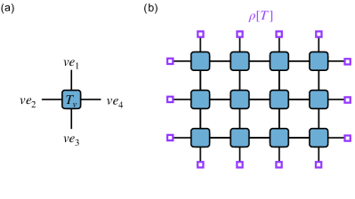
Figure 1: (a) A tensor $T_{v}$ at vertex $v$ with coordination number $z=4$. (b) Arranging the tensors in a network (taken to be square lattice here), we obtain a “tensor network state” $\rho[T]$ (see Eq. (4)) by contracting indicies on all bulk edges, as implemented by projecting onto the maximally entangled state $|{I_{e}}\rangle$. The state $\rho[T]$ is supported on the boundary qudits (highlighted by purple squares), and is in general unnormalized.

II.1 Review of Haar Case

Following Vasseur et al. (2019) we consider a Tensor Network with a set of vertices $v$, from each of which emerge $z$ edges $ve_{1},ve_{2},...,ve_{z}$, where $z$ is the coordination of the vertex (assumed to be the same for all vertices), see Fig. 1(a). We denote the bond dimension at each edge by $d$. At each vertex $v$ there is a quantum state described by a tensor

$$|T_{v}\rangle=\sum_{\mu_{ve_{1}},\mu_{ve_{2}},...,\mu_{ve_{z}}=1}^{d}\ \ \ {\left(T\right)}_{\mu_{ve_{1}},\mu_{ve_{2}},...,\mu_{ve_{z}}}\times\ \ \ \$$ (1)

$$\times|\mu_{ve_{1}}\rangle\otimes|\mu_{ve_{2}}\rangle\otimes...\otimes|\mu_{ve_{z}}\rangle=\sum_{\mu_{v}=1}^{D}\ \ T_{\mu_{v}}\ \ |\mu_{v}\rangle,$$

where we introduced the shorthand $\mu_{v}=$ $(\mu_{ve_{1}},\mu_{ve_{2}},...,\mu_{ve_{z}})$ for the collection of labels of the $D:=(d)^{z}$ basis elements at a vertex, $\mu_{v}=1,...D$. Defining a maximally entangled state on the edge $e:=\langle v,v^{\prime}\rangle$ connecting two adjacent vertices $v$ and $v^{\prime}$,

$$|I_{e}\rangle:={1\over\sqrt{d}}\sum_{\mu_{ve},\mu_{{v^{\prime}}e}=1}^{d}\delta_{\mu_{ve},\mu_{{v^{\prime}}e}}\ \ \ |\mu_{ve}\rangle\otimes|\mu_{{v^{\prime}}e}\rangle,$$ (2)

the (unnormalized) wave function of the Tensor Network is defined by

$$|\psi[T]\rangle:=\left(\otimes_{e}\langle I_{e}|\right)\left(\otimes_{v}|T_{v}\rangle\right)$$ (3)

where the tensor product is over all (bulk) edges and all vertices of the network, respectively. The object of interest is the (so-far still unnormalized) pure state density matrix of the network

$$\rho[T]:=|\psi[T]\rangle\ \langle\psi[T]|,$$ (4)

for the remaining degrees of freedom (‘dangling legs’ of the tensor network), which we will choose to be at the boundary of the network, see Fig. 1(b). Owing to the need to normalize the states of the PEPS wave function of the network (and to describe the $n$-th Rényi entropies for any integer $n$), it is necessary to work with the tensor product of $Q=nm$ copies of this (unnormalized) density matrix

$$\otimes^{Q}\rho[T]=\otimes^{Q}\Big{(}|\psi[T]\rangle\ \langle\psi[T]|\Big{)}.$$ (5)

More precisely, our goal is to compute the $n$th entanglement Renyi entropy of a subregion $A$ of the dangling (‘boundary’) legs of the tensor networks

$$S_{A}^{(n)}=\frac{1}{1-n}\ln\frac{{\rm tr}\rho^{n}_{A}}{({\rm tr}\rho)^{n}},$$ (6)

with $\rho_{A}={\rm tr}_{\overline{A}}\rho$ the reduced density matrix in the region $A$, and $\bar{A}$ the complement of $A$. The average of this quantity over the random tensors, to be defined more precisely below, can be computed from the replicated density matrix using

$$S_{A}^{(n)}=\frac{1}{1-n}\underset{m\to 0}{\rm lim}\frac{1}{m}\left(({\rm tr}\rho^{n}_{A})^{m}-({\rm tr}\rho^{\otimes Q})\right),$$ (7)

where $({\rm tr}\rho^{n}_{A})^{m}$ and ${\rm tr}\rho^{\otimes Q}$ differ only in the way the boundary legs are contracted.

The Haar Random Tensor Network is defined by letting the state $|\mu^{(i)}_{v}\rangle$ at each vertex $v$ in each (replica and Rényi) copy $i=1,...,Q$ arise from a fixed basis state in the $D$-dimensional Hilbert space associated with the vertex, by the action of the same unitary $D\times D$ matrix $U$ in each (replica and Rényi) copy, chosen randomly and independently at each vertex $v$ from the Haar ensemble. Explicitly, the tensor in (1) will then be of the form

$$T_{\mu_{v}}=\bra{\mu_{v}}\hat{U}\ket{1}\coloneqq{(U)}_{\mu_{v},1}.\qquad\mu_{v}=1,...,D.$$ (8)

The tensor factor contribution to (5) arising from the quantum states (1) at vertex $v$ will then be, using (3):

$$\otimes^{Q}\Big{(}|T_{v}\rangle\ \langle T_{v}|\Big{)}=\otimes^{Q}\Big{(}{\hat{U}}|1\rangle\ \langle 1|{\hat{U}}^{\dagger}\Big{)}=$$ (9)

$$=\sum_{\mu_{v}^{(i)},{\nu}_{v}^{(j)}}{U}_{1,{\mu}^{(1)}_{v}}...{U}_{1,{\mu}^{(Q)}_{v}}{U^{\dagger}}_{{\nu}^{(1)}_{v},1}...{U^{\dagger}}_{{\nu}^{(Q)}_{v},1}\times$$

$$\times(|\nu_{v}^{(1)}\rangle\otimes...\otimes|\nu_{v}^{(Q)}\rangle)\otimes(\langle{\mu}_{v}^{(1)}|\otimes...\otimes\langle{\mu}_{v}^{(Q)}|).$$

Specializing the familiar result for the average $\mathbb{E}_{U\in U(D)}\left[...\right]$ over the Haar measure $d\mu(U)$ Collins (2003)

$$\int_{\rm Haar}d\mu(U)\ \ U_{i_{1},j_{1}}...U_{i_{Q},j_{Q}}U^{\dagger}_{j^{\prime}_{1},i^{\prime}_{1}}...U^{\dagger}_{j^{\prime}_{Q},i^{\prime}_{Q}}=$$

$$=\sum_{\sigma,\tau\in S_{Q}}\ \ {\rm Wg}(\tau\sigma^{-1})\ \ \delta_{i_{1},i^{\prime}_{\sigma(1)}}...\delta_{i_{Q},i^{\prime}_{\sigma(Q)}}\delta_{j_{1},j^{\prime}_{\tau(1)}}...\delta_{j_{Q},j^{\prime}_{\tau(Q)}}$$

(10)

to the case where $i_{1}=...=i_{Q}=1$ and $i^{\prime}_{1}=...=i^{\prime}_{Q}=1$, yields

$$\mathbb{E}_{U\in U(D)}\left[U_{1,j_{1}}...U_{1,j_{Q}}U^{\dagger}_{j^{\prime}_{1},1}...U^{\dagger}_{j^{\prime}_{Q},1}\right]=$$

$$={1\over{\cal N}_{H}}\sum_{\tau\in S_{Q}}\ \ \delta_{j_{1},j^{\prime}_{\tau(1)}}...\delta_{j_{Q},j^{\prime}_{\tau(Q)}},$$

where ${1\over{\cal N}_{H}}=$ $\sum_{\sigma}{\rm Wg}_{D}(\sigma)=\prod_{k=1}^{Q}(D+k-1)^{-1}$. This implies that the Haar average of (9) gives a contribution coming from the vertex $v$ of the form

$$\mathbb{E}_{U\in U(D)}\bigg{[}\otimes^{Q}\Big{(}|T_{v}\rangle\langle T_{v}|\Big{)}\bigg{]}={1\over{\cal N}_{H}}\sum_{\tau\in S_{Q}}{\hat{R}}_{v}(\tau)$$ (11)

where

$${\hat{R}}_{v}(\tau):=\sum_{\vec{\boldsymbol{\mu}}_{v}}\ \ |{\hat{\tau}}({\vec{\boldsymbol{\mu}}_{v}})\rangle\ \ \langle{\vec{\boldsymbol{\mu}}_{v}}|,\qquad\tau\in S_{Q}$$ (12)

and where $\vec{\boldsymbol{\mu}}_{v}=$ $({\mu}_{v}^{(1)},{\mu}_{v}^{(2)},...,{\mu}_{v}^{(Q)})$ labels an orthonormal basis of the $Q$ (replica and Rényi) copies of the $D$-dimensional Hilbert space, $({{\bf C}^{D}})^{Q}$, at vertex $v$. Here $S_{Q}$ denotes the permutation group of $Q$ elements, and ${\hat{\tau}}$ is the operator that permutes the $Q$ factors of the tensor product,

$$|\vec{\boldsymbol{\mu}}_{v}\rangle :=|{\mu}_{v}^{(1)},{\mu}_{v}^{(2)},...,{\mu}_{v}^{(Q)}\rangle,$$ (13)

$$|{\hat{\tau}}(\vec{\boldsymbol{\mu}}_{v})\rangle :=|{\mu}_{v}^{(\tau(1))},{\mu}_{v}^{(\tau(2))},...,{\mu}_{v}^{(\tau(Q))}\rangle.$$

The operator ${\hat{R}}_{v}(\tau)$ in (12) is simply the permutation operator permuting the $Q$ (replica and Rényi) copies of the vector space ${\bf C}^{D}$ at vertex $v$. Equation (11) is the key result for the Haar case. The operator ${\hat{R}}_{v}(\tau)$ in (12) commutes with the action of all unitaries $U\in U(D)$ on the tensor product $({\bf C}^{D})^{Q}$ associated with a vertex. Viewing the set of operators ${\hat{R}}(\tau)$ where $\tau$ runs over all permutations in the group $S_{Q}$ as a basis of a (complex) linear vector space, it can be shown that this vector space of operators forms the set of all operators commuting with the action of the unitaries on the tensor product $({\bf C}^{D})^{Q}$. This set of operators is called the commutant of action of the unitary group on the tensor product, and the stated result is known as the famous statement of Schur-Weyl duality.

Consider now a single edge $e$ emanating from a vertex $v$. We label an orthonormal basis of the $Q$ (replica and Rényi) copies of the $d$-dimensional Hilbert space of edge $e$ at vertex $v$ by $\vec{\mu}_{ve}=$ $(\mu_{ve}^{(1)},\mu_{ve}^{(2)},...,\mu_{ve}^{(Q)})$, corresponding to the kets

$$|\vec{\mu}_{ve}\rangle:=|{\mu}_{ve}^{(1)},{\mu}_{ve}^{(2)},...,{\mu}_{ve}^{(Q)}\rangle.$$ (14)

Recalling the decomposition from (1),

$$|\mu_{v}\rangle=|\mu_{ve_{1}}\rangle\otimes|\mu_{ve_{2}}\rangle\otimes...\otimes|\mu_{ve_{z}}\rangle,$$ (15)

valid in each (replica and Rényi) copy, as well as (13), we see that the operator in (12) is the tensor product of operators

$${\hat{R}}_{e}(\tau),$$ (16)

defined on the edges $e$ of the vertex $v$, where

$${\hat{R}}_{e}(\tau):=\sum_{\vec{\mu}_{ve}}\ \ |{\hat{\tau}}({\vec{\mu}_{ve}})\rangle\ \ \langle{\vec{\mu}_{ve}}|,\qquad\tau\in S_{Q}$$ (17)

and ${\hat{\tau}}$ labels the operator that permutes the $Q$ (replica and Rényi) copies of the $d$-dimensional Hilbert space, $({{\bf C}^{d}})^{Q}$, at an edge $e$ at vertex $v$

$$|\vec{\mu}_{ve}\rangle :=|{\mu}_{ve}^{(1)},{\mu}_{ve}^{(2)},...,{\mu}_{ve}^{(Q)}\rangle$$

$$|{\hat{\tau}}(\vec{\mu}_{ve})\rangle :=|{\mu}_{ve}^{(\tau(1))},{\mu}_{ve}^{(\tau(2))},...,{\mu}_{ve}^{(\tau(Q))}\rangle.$$ (18)

In other words, we have

$${\hat{R}}_{v}(\tau)=\bigotimes_{e=1}^{z}{\hat{R}}_{e}(\tau)=[{\hat{R}}_{e}(\tau)]^{\otimes z}.$$ (19)

Consider now two adjacent vertices $v$ and $v^{\prime}$ connected by an edge $e$. The contribution to (5) arising from the edge joining adjacent vertices $v$ (permutation $\tau$) and $v^{\prime}$ (permutation $\sigma$) is then from (3) and (5)

$$\left(\otimes^{Q}\langle I_{e}|\right)\ {\hat{R}}_{e}(\tau){\hat{R}}_{e}(\sigma)\ \left(\otimes^{Q}|I_{e}\rangle\right)=$$ (20)

$$={1\over d^{Q}}\sum_{\vec{\mu}_{ve},\vec{\mu}_{v^{\prime}e}}\ [{\hat{R}}_{e}(\tau)]_{\vec{\mu}_{ve},\vec{\mu}_{v^{\prime}e}}[{\hat{R}}_{e}(\sigma)]_{\vec{\mu}_{v^{\prime}e},\vec{\mu}_{ve}}=$$

$$={1\over d^{Q}}{\rm tr}\left[{\hat{R}}_{e}(\tau){\hat{R}}^{\dagger}_{e}(\sigma)\right]={1\over d^{Q}}{\rm tr}\left[{\hat{R}}_{e}(\tau\sigma^{-1})\right].$$

It is seen by inspectionVasseur et al. (2019) (using definition (17)) that

$${\rm tr}\left[{\hat{R}}_{e}(\tau\sigma^{-1})\right]=e^{\ \ln(d)\ C(\tau\sigma^{-1})\ },$$ (21)

where $C(\tau)$ denotes the number of cycles in the permutation $\tau\in S_{Q}$. Once the product over the analogous contributions from all edges and vertices is taken, a sum over all independent permutations $\sigma_{v}$ in the group $S_{Q}$ at all vertices $v$ has to be performed. This yields the (bulk) partition function of the Haar Stat Mech model Vasseur et al. (2019), whose ‘spins’ are the elements of the permutation group located at the vertices,

$$Z_{\emptyset}=\mathbb{E}_{U\in U(D)}\ {\rm tr}\rho^{\otimes Q}=\prod_{\{\sigma_{v}\}}\ \ \exp\{-\sum_{\langle v,v^{\prime}\rangle}\ {\cal H}(\sigma_{v},\sigma_{v^{\prime}})\},$$

$${\cal H}(\sigma_{v},\sigma_{v^{\prime}})=\ln(d)|\sigma_{v},\sigma_{v^{\prime}}|:=\ln(d)\ [Q-C(\sigma_{v}\sigma^{-1}_{v^{\prime}}],\ \ \$$ (22)

where we can think of $|\sigma_{v},\sigma_{v}|$, defined above, as a ‘metric’ on permutations. – We now see that the fact that the degrees of freedom (the ‘spins’) of the RTN model of random Haar tensors are the elements of the permutation group arises from the fact that the permutations form a basis of the commutant of the action of the unitaries on the tensor product Hilbert space. The permutation degrees of freedom at the end of the dangling boundary legs are fixed, and dictated by the trace under consideration. In order to compute $Z_{\emptyset}=\mathbb{E}_{U\in U(D)}\ {\rm tr}\rho^{\otimes Q}$, the boundary permutations are fixed to the identity, corresponding to contracting each replica with itself. On the other hand, one can compute $Z_{A}=\mathbb{E}_{U\in U(D)}({\rm tr}\rho^{n}_{A})^{m}$ by fixing the same identity permutation in the region ${\bar{A}}$, while fixing $g_{\rm SWAP}=(12\dots n)^{\otimes m}$ in the region $A$ in order to compute the partial trace.

In the sequel, we will identify, using the same logic, the degrees of freedom (i.e. the ‘spins’) of the RTN model for random Clifford tensors Nezami and Walter (2020); Yang et al. (2021). Analogously, they will form a basis of the commutant of the action of the Clifford unitaries on the $Q$-fold tensor product. Since Clifford unitary tensors form a subgroup of all (Haar) unitary tensors, the set of operators that will commute with their action on the tensor Hilbert space will the larger. In other words, the commutant with will be larger as compared to the Haar case. We will now proceed to explain the nature of this larger commutant, and thus of the spins of the Stat. Mech. model for the RTN model of random Clifford tensors.

II.2 Schur-Weyl Duality for the Clifford RTN model

Throughout this subsection (and any discussion of the RTN or monitored quantum circuits with random Clifford unitaries in this paper) we will take the on-site Hilbert space dimension $d$ at each edge to be a power of a prime number $p$, i.e. $d=p^{M}$ with some integer $M$.

The difference with the case of Haar unitary tensors appears in (8): In the Clifford case the matrix $U$ is replaced by a unitary matrix, which we will denote by $V$, in the Clifford subgroup ${\rm Cliff}(N,p)$ of all unitary $D\times D$ matrices $U(D)$, where $D=d^{z}=p^{zM}=p^{N}$, and $N=zM$. First, we will use this setup to describe the commutant of this action on the $Q$-fold tensor product space. Second, after the description of the commutant is completed, we will consider the generalization of the average (11) to a random average over all the elements of this Clifford subgroup ${\rm Cliff}(N,p)$ acting on a fixed tensor $|T_{v}\rangle$ which is now chosen to be a stabilizer state.

For the first step, the key statement of Schur-Weyl duality for the Clifford group is that there is a specific generalization of the operators (12) spanning the commutant, which are no longer characterized by permutations.

II.2.1 Description of properties of the Commutant

Specifically, we will be interested in the basis $|\vec{\boldsymbol{\mu}}_{v}\rangle$ of the $Q$-fold tensor product space $({\bf C}^{D})^{Q}$ of all $z$ edges emerging from a given vertex $v$, so that we can write $({\bf C}^{D})^{Q}=$ $(({\bf C}^{p})^{\otimes N})^{\otimes Q}$ where $N=M\cdot z$. The $p$ basis elements of the vector space ${\bf C}^{p}$ can be labeled by the $p$ elements of ${\bf Z}_{p}:=$ ${\bf Z}/(p\cdot{\bf Z})=$ $0,1,2,...,(p-1)$ i.e. by the set of integers modulo $p$ (the “computational basis”). It will soon become important that the set ${\bf Z}_{p}$ forms a number field which is often also denoted by ${\bf F}_{p}={\bf Z}_{p}$.

Let us first consider the simplest case where $N=1$, i.e. of the $Q$-fold tensor product $({\bf C}^{p})^{\otimes Q}$, which turns out to be the most important case, underlying all others. The same unitary $p\times p$ matrix $V$ in the Clifford subgroup ${\rm Cliff}(1,p)$ of the unitary group $U(p)$ acts simultaneously on each of the $Q$ factors of the tensor product, generalizing (8) with $D$ replaced by $p$. Since the basis elements of ${\bf C}^{p}$ are labeled (as above) by elements $\mu\in{\bf Z}_{p}={\bf F}_{p}$, the elements of a basis of $({\bf C}^{p})^{\otimes Q}$ will be labeled by $Q$-dimensional (say: column-) vectors with entries in ${\bf Z}_{p}=$ ${\bf F}_{p}$, written as usual as elements of $({\bf Z}_{p})^{Q}=$ $({\bf F}_{p})^{Q}$, i.e. by vectors $\vec{\mu}=$ $(\mu^{(1)},\mu^{(2)},...,\mu^{(Q)})^{t}$. In other words, every $Q$-dimensional (column) vector with entries in ${\bf Z}_{p}=$ ${\bf F}_{p}$, i.e. every (column) vector in $({\bf Z}_{p})^{Q}=$ $({\bf F}_{p})^{Q}$, denotes a basis element of the vector space $({\bf C}^{p})^{Q}$.

The main result of Gross et al. (2021) is that in this case the generalization of (12) and (17), i.e. of the operators which in the Haar case formed a basis of the commutant, i.e. of the set (actually the vector space) of all operators commuting with the action of the unitary group on the tensor product, in the Clifford case is based on the operators

$${\hat{r}}(T)=\sum_{(\vec{\nu},\vec{\mu})\in T}\ |\vec{\nu}\rangle\ \langle\vec{\mu}|,$$ (23)

where $T$ runs over a certain set (to be specified below) of subspaces of $({\bf Z}_{p})^{Q}\oplus({\bf Z}_{p})^{Q}$. In other words, the permutation in the Haar case is now replaced by the (more general) object $T$. The so-defined ${\hat{r}}(T)$ is clearly an operator acting on $({\bf C}^{p})^{Q}$. The set of allowed subspaces $T$, denoted by $\Sigma_{Q}(p)$ and to be specified below, forms the commutant in the Clifford case.

In order to appreciate the meaning of (23), let us first look at a special case: Since the set of all Clifford unitary matrices $V\in{\rm Cliff}(1,p)$ forms a subgroup of the set of all unitary matrices $U\in U(p)$, the set of all operators commuting with the action of all Clifford unitaries on the $Q$-fold tensor product of the Hilbert space ${\bf C}^{p}$ must be a larger set than the set of all those commuting with the action of all unitaries $U$. Since we know from the previous section on the Haar case that the commutant in the latter case is spanned by all permutations $\tau\in S_{Q}$, the operators that appeared in (12) and (17) must form a subset of the set of operators described in (23). Indeed, choosing the subspace of $({\bf Z}_{p})^{Q}\oplus({\bf Z}_{p})^{Q}$ to be of the special form

$$T=\{({\hat{\tau}}(\vec{\mu}),\vec{\mu}):\ \ \vec{\mu}\in({\bf Z}_{p})^{Q}\}$$ (24)

reproduces precisely the previous expression from (12) and (17), where in the above equation ${\hat{\tau}}$ acts by permuting the $Q$ rows of the column vector $\vec{\mu}$.

Before we move on to the description of the commutant and its properties for the Clifford case , we state an important stabilization property Gross et al. (2021) that says that, once the prime number $p$ is fixed, this commutant does not depend on the dimension of the (on-site) Hilbert space on which it acts, as long as that dimension is large enough. This is a very important statement because it says that, for a fixed prime $p$, the specific form of the commutant that we describe below is universally valid, independent of the (sufficiently large) prime-power dimension of Hilbert space it acts on. For this purpose, we consider a general on-site Hilbert space $({\bf C}^{p})^{N}$ of dimension $D=p^{N}$ (as above), i.e. simply the $N$-fold tensor product of the Hilbert space ${\bf C}^{p}$ discussed above. We now consider as before the tensor product of $Q$ (replica, and Rényi) copies of this $D$-dimensional Hilbert space, i.e. $[({\bf C}^{p})^{N}]^{\otimes Q}=$ $({\bf C}^{p})^{N\cdot Q}$, and on each of the $Q$ copies of the $D=p^{N}$-dimensional vector space $({\bf C}^{p})^{N}$ acts the same unitary $D\times D$ matrix $V$ in the Clifford subgroup ${\rm Cliff}(N,p)$ of the unitary group $U(D)$. Now the following statement holds:

-: Stabilization property Gross et al. (2021)

The number of linearly independent operators (which will span the commutant) that commute with the action of the same Clifford unitary matrices $V\in{\rm Cliff}(N,p)$ acting on each of the $Q$ factors of the $Q$-fold tensor product, $[({\bf C})^{D}]^{\otimes Q}$, where $D=p^{N}$ ($p=prime$), is independent of $N$ as long as $N\geq(Q-1)$.

Moreover, these linearly independent operators are simply

$${\hat{R}}(T)=[{\hat{r}}(T)]^{\otimes N},\qquad{\rm where}\ T\in\Sigma_{Q}(p),$$ (25)

i.e. they are nothing but the $N$-fold tensor products of the operators introduced in (23) above. Note that these operators are thus uniquely determined by the set $\Sigma_{Q}(p)$, independent of the power $N$ determining the Hilbert space dimension $D=p^{N}$, as long as $N$ is large enough (as specified above).

The key result of Gross et al. (2021) is a complete characterization of the set $\Sigma_{Q}(p)$ of subspaces $T$ appearing in (25), which describes the commutant of the Clifford action on the $Q$-fold tensor product. A more detailed summary of this is given in App. A. Here we just list those properties of the commutant $\Sigma_{Q}(p)$ that appear directly in the formulation of the Clifford RTN model. These are a metric on the commutant, and the invariance of this metric under a certain symmetry group. We now proceed to discuss these two properties.

An important property of the commutant $\Sigma_{Q}(p)$ is that it contains a group as a subset (though, $\Sigma_{Q}(p)$ is in general larger than this group, and does in general not form a group). This group is the group of all orthogonal $Q\times Q$ matrices $O$ with elements in the number field ${\bf Z}_{p}=$ ${\bf F}_{p}$ which satisfy besides the “orthogonality condition” $O^{t}O=OO^{t}={\boldsymbol{I}}_{Q}$ (the $Q\times Q$ identity matrix) also the additional condition of “being stochastic”, meaning that the column vector $1_{Q}$ whose entries are all the number $1\in{\bf F}_{p}$, is invariant under the action of the matrix $O$, as well as of its transpose, i.e. $O~{}1_{Q}=O^{t}~{}1_{Q}=1_{Q}$. The set of such matrices forms a group denoted by ${\cal O}_{Q}(p)$, the so-called stochastic orthogonal group. Note that [in connection with the discussion around (24)] the permutation group $S_{Q}$ is a subgroup of ${\cal O}_{Q}(p)$, namely it corresponds to the set of those $Q\times Q$ matrices which have only one $1\in{\bf F}_{p}$ in each row and each column; those matrices clearly implement permutations.

For the formulation of the Clifford Stat Mech model we use the fact that there exists a metric on the commutant: Namely, that for any two elements $T_{a}$ and $T_{b}$ of the commutant $\Sigma_{Q}(p)$ there exists a metric which arises from the trace

$$W(T_{a},T_{b}):={\rm tr}\left[{{\hat{R}}^{\dagger}}(T_{a}){\hat{R}}(T_{b})\right]=(p^{N})^{Q-|T_{a},T_{b}|},\ \ \ \$$ (26)

for any $T_{a},T_{b}\in\Sigma_{Q}(p)$, where ${\hat{R}}(T)$ is defined in (25). The metric satisfies the usual properties $|T_{a},T_{b}|\geq 0,$ $|T_{a},T_{b}|=|T_{b},T_{a}|$, and $|T_{a},T_{b}|=0$ if and only if $T_{a}=T_{b}$.

The other property we need is that the metric in (26) is invariant under the action of the direct product of two copies of the stochastic orthogonal group ${\cal O}_{Q}(p)\times{\cal O}_{Q}(p)$, acting as

$$|T_{1},T_{2}|=|T^{\prime}_{1},T^{\prime}_{2}|,\ \ \ {\rm where}\ \ T_{1},T_{2}\in\Sigma_{Q}(p),$$

$${\rm and}$$

$$T^{\prime}_{1}=O_{L}T_{1}O_{R}^{-1},\ T^{\prime}_{2}=O_{L}T_{2}O_{R}^{-1},\ {\rm with}\ O_{L},O_{R}\in{\cal O}_{Q}(p).$$

II.2.2 Stat Mech model for the Clifford (Stabilizer) RTN

The construction of the Clifford RTN follows the same steps as those reviewed in Sect. II.1 for Haar unitaries. We consider the RTN where on each edge there is an “on-site” Hilbert space $({\bf C}^{p})^{M}$ of dimension $d=p^{M}$ of $M$ qudits, each qudit having a $p$-dimensional Hilbert space where $p$ is a prime number. (For a brief review, see e.g. App. B.) In complete analogy with Sect. II.1, a Hilbert space $({\bf C}^{p})^{M\cdot z}=$ $({\bf C}^{p})^{N}$ of dimension $D=p^{N}$ where $N=M\cdot z$ is associated with each vertex $v$, where $z$ is the coordination number of a vertex.

Specifically, in the Clifford case the first line of (9) will be replaced by

$$\otimes^{Q}\Big{(}|T_{v}\rangle\ \langle T_{v}|\Big{)}=\otimes^{Q}\Bigg{(}\left({\hat{V}}|0\rangle^{\otimes N}\right)\ \left(\langle 0|^{\otimes N}{\hat{V}}^{\dagger}\right)\Bigg{)},\ \ \$$ (28)

where ${\hat{V}}$ is an element of the Clifford group ${\rm Cliff}(N,p)$ acting on the Hilbert space $({\bf C}^{p})^{N}$ at vertex $v$. This means simply that each of the states $|1\rangle$ that appear in each of the $Q$ tensor factors in (9) is replaced by the state $|0\rangle^{\otimes N}\in{\bf C}^{N}$ which is written in the computational basis, where $0\in{\bf F}_{p}$ denotes the number zero in the finite number field ${\bf F}_{p}$. [See, e.g., the paragraph preceeding that containing (23), or App. B.] The reason why $|0\rangle^{\otimes N}$ is chosen at each vertex is because this state is a stabilizer state. Owing to the fact that this state is a stabilizer state, the average of (28) over the Clifford group at a vertex $v$ is (as shown in Gross et al. (2021)) an equal-weight superposition over elements of the commutant [see, e.g., (73) of App. B]:

$$\mathbb{E}_{{\hat{V}}\in{\rm Cliff}(N,p)}\left[\otimes^{Q}\Bigg{(}\left({\hat{V}}|0\rangle^{\otimes N}\right)\ \left(\langle 0|^{\otimes N}{\hat{V}}^{\dagger}\right)\Bigg{)}\right]=$$

$$={1\over Z_{n,p,Q}}\sum_{T_{v}\in\Sigma_{Q}(p)}{\hat{R}}_{v}(T_{v})$$ (29)

where

$${\hat{R}}_{v}(T)=\left[{\hat{R}}_{e}(T)\right]^{\otimes z},\ {\rm with}\ {\hat{R}}_{e}(T)=\left[{\hat{r}}(T)\right]^{\otimes M}.$$

Then, in complete analogy with (20), one obtains using a maximally entangled state in an orthonormal basis on each edge, a contribution to the partition function from that edge of the form

$${1\over(p^{M})^{Q}}{\rm tr}\left[{\hat{R}}^{\dagger}_{e}(T_{v}){\hat{R}}_{e}(T_{v^{\prime}})\right]=(p^{M})^{-|T_{v},T_{v^{\prime}}|},$$

where $T_{v}$ and $T_{v^{\prime}}$ denote elements of the commutant from the equal-weight sums (29) at the two vertices $v$ and $v^{\prime}$ connected by the edge $e$. Then we obtain, by collecting all terms from the equal-weight sums appearing at each edge, in complete analogy to (II.1), the following (bulk) partition function of the Clifford RTN model

$$Z_{\emptyset}=\mathbb{E}_{{\hat{V}}\in{\rm Cliff}(M,p)}\ {\rm tr}\rho^{\otimes Q}=$$ (30)

$$=\prod_{\{T_{v}\in\Sigma_{Q}(p)\}}\ \ \exp\{-\sum_{\langle v,v^{\prime}\rangle}\ {\cal H}(T_{v},T_{v^{\prime}})\},$$

$${\cal H}(T_{v},T_{v^{\prime}})=\ln(p^{M})\ |T_{v},T_{v^{\prime}}|.$$ (31)

Observables, including the entanglement entropy, are formulated in the same way as in the Haar case. [See (5), (6), (7), and the discussion below (II.1).]

We recall from Vasseur et al. (2019) that the transition in the RTN model can be driven by making (at each edge) the bond dimension random. In the Clifford case, this means that the bond dimension is $D_{\rm bond}=p^{M}$ with $p={\rm prime}=$ fixed, where $M$ is independently distributed at each edge according to some probability distribution. A simple choice for this would be random dilution, corresponding to a binary probability distribution for $M$, taking on two values $M=0$ and $M=M_{0}=$ fixed at random. This would drive a transition in the RTN model corresponding to the (same) universality class possessing (see below) symmetry group ${\cal O}_{Q}(p)\times{\cal O}_{Q}(p)$ for any choice of a (large enough) value $M_{0}$.

We stress that owing to the invariance property (II.2.1) of the metric, the Clifford Stat Mech model is invariant under the ${\cal O}_{Q}(p)\times{\cal O}_{Q}(p)$ symmetry group. Note that this is a different symmetry group for different primes $p$, but that this symmetry group is the same for all on-site Hilbert space dimensions $d=p^{M}$ for a fixed prime $p$, independent of $M$: the symmetry group depends only on the prime $p$. This thus implies that any universal quantities occurring at continuous phase transitions in this Stat. Mech. model will in general depend on the prime $p$, but will be the same for all on-site Hilbert space dimensions $d=p^{M}$ of the same prime number $p$, independent of $M$. – Note that this is in contrast to the Haar case, where the same universality class occurs for the transition at any finite on-site Hilbert space dimension. In the Haar case, this must of course be the case, because universal properties cannot depend on short-distance (“ultraviolet”) physics - all those Stat. Mech. models have the same symmetry. While this feature is the same in the Clifford case for a fixed value of the prime $p$ (i.e., for on-site Hilbert space dimension $d=p^{M}$ and different values of $M$), RTN models possessing on-site Hilbert space dimensions which are powers of different primes have in general different universal critical properties at continuous phase transitions, because they are invariant under different symmetry groups.

III Measurement-induced phase transition in Clifford circuits

III.1 Setup and replica trick

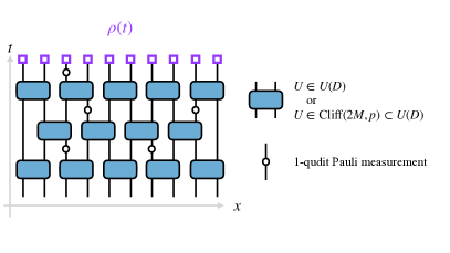
Figure 2: The architecture of the monitored quantum circuit model. Each blue block represents a random unitary gate, and each hollowed circle represents a rank-1 projective measurement, occuring randomly with probability $p_{0}$. The dynamical state $\rho(t)$ at circuit depth $t$ is supported on qudits at the final time step (highlighted with purple squares), and is labeled by the the measurement record $\mathbf{m}$, see Eq. (32). We consider two cases, depending on whether the random unitaries are sampled from the Haar measure on $U(D=2d)$ (the “random Haar circuit”), or from the uniform distribution the Clifford group $\mathrm{Cliff}(2M,p)\subset U(D)$ (the “random Clifford circuit”).

We now turn to measurement-induced entanglement transitions in monitored quantum circuits. We consider a one-dimensional chain of qudits with on-site Hilbert space dimension $d$, subject to discrete-time dynamics generated by a quantum circuit with a ‘brick-wall’ pattern, as illustrated in Fig. 2. Each unitary gate is acting on a pair of neighboring qudits, and will be drawn from the Clifford group (we will also briefly review the Haar case below). After each layer of the circuit (single time step), every site is either measured (projectively) with probability $p_{0}$, or left untouched with probability $1-p_{0}$. For a fixed set of unitary gates and measurement locations, the hybrid non-unitary dynamics of the system is described through the quantum channel

$$\rho(t)=\sum_{\mathbf{m}}K_{\mathbf{m}}\rho K^{\dagger}_{\mathbf{m}},$$ (32)

where $\rho$ is the system’s density matrix, $\mathbf{m}$ denotes measurement outcomes, and $K_{\mathbf{m}}$ are Kraus operators consisting of the random unitary gates and the projectors onto the measurement outcomes. We are interested in the entanglement properties of individual quantum trajectories $\rho_{\mathbf{m}}=K_{\mathbf{m}}\rho K^{\dagger}_{\mathbf{m}}$, which occur with the Born probability $p_{\mathbf{m}}={\rm tr}\rho_{\mathbf{m}}$. Our goal is to compute the Renyi entropy of such single trajectories, averaged over measurement outcomes and random unitary gates

$$S_{A}^{(n)}=\mathbb{E}_{U}\sum_{\mathbf{m}}p_{\mathbf{m}}\frac{1}{1-n}\ln\frac{{\rm tr}\rho^{n}_{A,{\mathbf{m}}}}{({\rm tr}\rho_{\mathbf{m}})^{n}}.$$ (33)

Ultimately, we also want to average over measurement locations, and denote $\overline{S_{A}^{(n)}}$ the Renyi entropy averaged over measurement locations as well. As in the random tensor networks section above, we follow Refs Vasseur et al. (2019); Zhou and Nahum (2019); Bao et al. (2020); Jian et al. (2020) and use a replica trick to compute (33):

$$S_{A}^{(n)}=\mathbb{E}_{U}\sum_{\mathbf{m}}\underset{m\to 0}{\rm lim}\frac{{\rm tr}\rho_{\mathbf{m}}}{(1-n)m}\left(({\rm tr}\rho^{n}_{A,{\mathbf{m}}})^{m}-({\rm tr}\rho_{\mathbf{m}}^{\otimes mn})\right).$$ (34)

We will write $Q=nm+1$ the number of replicas, where the additional replica compared to the random tensor networks case comes from the Born probability weighting different quantum trajectories.

III.2 Generalized Weingarten functions

III.2.1 Haar case

Let us first briefly summarize the main ingredient of the statistical mechanics model of the measurement-induced transition, with Haar random unitary gates acting on qudits. Upon replicating the model, averaging over Haar gates drawn from the unitary group $U(D=d^{2})$ naturally leads to degrees of freedom living in the permutation group $S_{Q}$, with $Q=nk+1$ the number of replicas. This follows from the Schur-Weyl duality detailed in the previous section, which states that the permutation group $S_{Q}$ and the unitary group $U(D)$ act on $({\bf C}^{D})^{\otimes Q}$ as a commuting pair. The Haar average of the replicated unitaries is given by (see Appendix C)

$$\mathbb{E}_{U\in U(D)}\left(U^{*Q}\otimes U^{Q}\right)=\sum_{\sigma,\tau\in S_{Q}}\text{Wg}_{D}(\sigma^{-1}\tau){\hat{R}}_{v}(\sigma)\otimes{\hat{R}}_{v}(\tau),$$ (35)

where Wg are Weingarten functions, $D=d^{2}$, ${\hat{R}}_{v}(\sigma)={\hat{R}}_{e}(\sigma)\otimes{\hat{R}}_{e}(\sigma)$ (see eq. (12)) permutes the output legs of $U$ by $\sigma$, and contracts them with the corresponding legs of $U^{*}$ (and similarly for $\hat{R}_{v}(\tau)$ acting on the input legs). The tensor product in the right-hand side of eq. (35) is over output and input legs of the unitary. Now contrary to the previous section on random tensor networks, the Weingarten function will directly enter the Boltzmann weights of the statistical models. As we review in Appendix C, those functions satisfy

$$\sum_{\tau\in S_{Q}}\text{Wg}_{D}(\sigma^{-1}\tau)D^{C(\tau)}=\delta_{\sigma,1},$$ (36)

where we recall that $C(\tau)$ denotes the number of cycles in the permutation $\tau$. This implies that the Weingarten function is the inverse of the cycle counting function $D^{C(\tau)}$. Equation (35) naturally defines the degrees of freedom of the statistical model living on a honeycomb lattice (Fig. 3), where permutations live on vertices. Contracting unitary gates can be done by assigning a weight to links connecting unitaries given by

$$W(\sigma,\tau)={\rm tr}\ \big{[}{\hat{R}}_{e}^{\dagger}(\sigma){\hat{R}}_{e}(\tau)\big{]}=d^{C(\sigma^{-1}\tau)}.$$ (37)

Note the factor of $d$ here, instead of $D$, since we are focusing on a single leg of the unitary. This weight is associated to all links that were not measured. If a link was measured instead, all replicas are constrained to be in the same state, and the weight is instead $d$ after averaging over possible measurement outcomes. Those equations fully determine the weights of the statistical model in monitored Haar random circuits. Upon averaging over measurement locations and outcomes, the weight assigned to a link is therefore given by Jian et al. (2020)

$$W_{p}(\sigma,\tau)=(1-p_{0})d^{C(\sigma^{-1}\tau)}+p_{0}d.$$ (38)

Putting these results together, we obtain an anisotropic statistical mechanics model defined on the honeycomb lattice,

$$Z=\sum_{\{g_{i}\in S_{Q}\}}\prod_{\langle ij\rangle\in G_{s}}W_{p}(\sigma_{i}^{-1}\tau_{j})\prod_{\langle ij\rangle\in G_{d}}\text{Wg}_{D}(\sigma_{i}^{-1}\tau_{j}),$$ (39)

where $G_{s}$ ($G_{d}$) denotes the set of solid (dashed) links on the lattice. In Fig. 3, the vertical (dashed) links on the honeycomb lattice represent the Weingarten functions which originated from averaging the two-site unitary gates, and the solid links keep track of the link weights originating from averaging over measurements.

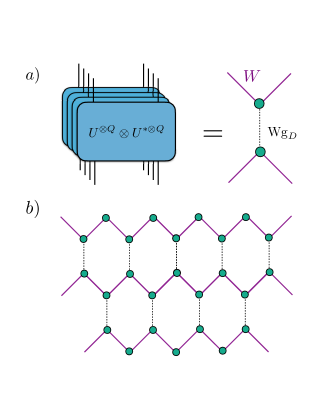
Figure 3: Statistical mechanics model for monitored quantum circuits. (a) The average over replicated unitary gates leads to degrees of freedom belonging to the commutant, defined on vertices; Weingarten weights $\text{Wg}_{D}$, represented by the dashed line; and link weights $W$, corresponding to purple solid lines. (b) The statistical mechanics model is defined on an anisotropic honeycomb lattice.

III.2.2 Clifford case

Let us now turn to the Clifford case, with random unitary gates drawn from the Clifford group ${\rm Cliff}(N,p)\subset U(D)$, with $D=d^{2}$, $N=2M$ and $d=p^{M}$ with $p$ prime. As in the Haar case, the average over Clifford gates is given in terms of tensor products of elements of the commutant of the Clifford group (see Appendix D)

$$\mathbb{E}_{U\in{\rm Cliff}(N,p)}\left(U^{*Q}\otimes U^{Q}\right)=$$

$$\sum_{T_{i},T_{o}\in\Sigma_{Q}(p)}\text{Wg}_{D}(T_{i},T_{0})\ {\hat{R}}_{v}(T_{o})\otimes{\hat{R}}_{v}(T_{i}),$$ (40)

where as before, ${\hat{R}}_{v}(T_{i})={\hat{R}}_{e}(T_{i})\otimes{\hat{R}}_{e}(T_{i})$ is acting on incoming legs, while ${\hat{R}}_{e}(T_{o})$ acts on outgoing legs, where the operator ${\hat{R}}_{e}={\hat{r}}^{\otimes M}$ was introduced in the previous section, see eq (23). Here the coefficients $\text{Wg}_{D}(T_{i},T_{0})$ are generalized Weingarten weights. The procedure to determine them follows closely the Haar case, and we show in Appendix D that the generalization of eq. (36) reads

$$\sum_{T_{b}\in\Sigma_{Q}(p)}\text{Wg}_{D}(T_{a},T_{b})\ {\rm tr}\big{[}\hat{R}_{v}^{\dagger}(T_{b})\hat{R}_{v}(T_{c})\big{]}=\delta_{T_{a},T_{c}},$$ (41)

as well as $\sum_{T_{b}\in\Sigma_{Q}(p)}{\rm tr}\big{[}\hat{R}_{v}^{\dagger}(T_{a})\hat{R}_{v}(T_{b})\big{]}\ \text{Wg}_{D}(T_{b},T_{c})=\delta_{T_{a},T_{c}}$. In other words, the Weingarten weights (when viewed as a matrix) are given by the inverse of the matrix ${\rm tr}\big{[}\hat{R}_{v}^{\dagger}(T_{a})\hat{R}_{v}(T_{b})\big{]}$. On the other hand, the link weights connecting two vertices are given by

$$W(T_{a},T_{b})={\rm tr}\big{[}{\hat{R}}_{e}^{\dagger}(T_{a}){\hat{R}}_{e}(T_{b})\big{]}=d^{Q-|T_{a},T_{b}|},$$ (42)

with $d=p^{M}$. As in the Haar case, this weight is replaced by a factor of $d$ if a measurement occurred on that link (upon averaging over measurement outcomes), as the measurement constrains all replicas to be in the same state. After averaging over measurement locations, the weight assigned to a link reads

$$W_{p}(T_{a},T_{b})=(1-p_{0})d^{Q-|T_{a},T_{b}|}+p_{0}d.$$ (43)

The partition function of the statistical model in the Clifford case is then given by

$$Z=\sum_{\{T_{i}\in\Sigma_{Q}(p)\}}\prod_{\langle ij\rangle\in G_{s}}W_{p}(T_{i},T_{j})\prod_{\langle ij\rangle\in G_{d}}\text{Wg}_{D}(T_{i},T_{j}),$$ (44)

with the same lattice as in the Haar case (44).

Note that both the link and Weingarten weights are invariant under two copies of the stochastic orthogonal group ${\cal O}_{Q}(p)\times{\cal O}_{Q}(p)$, acting as $T^{\prime}_{a}=O_{L}T_{a}O_{R}^{-1},\ T^{\prime}_{b}=O_{L}T_{b}O_{R}^{-1}$, with $O_{L},O_{R}\in{\cal O}_{Q}(p)$. The conclusions for the Clifford RTN statistical mechanics model thus carry over to Clifford monitored quantum circuits: the Clifford Stat. Mech. model is invariant under a global ${\cal O}_{Q}(p)\times{\cal O}_{Q}(p)$ symmetry group. This symmetry group depends only on the prime number $p$, and not on $M$ in the on-site Hilbert space dimension $d=p^{M}$. This implies that all universal quantities of the entanglement transition in Clifford monitored circuits will depend on $p$, but will be independent of $M$. This is in sharp contrast to the Haar case, where the same universality class occurs for the transition at any finite on-site Hilbert space dimension. Although the statistical mechanics model (44) describing the monitored Cliffod circuit has the same symmetry group as the one describing stabilizer RTNs (II.2.2), both problems correspond to different replica limits: $Q\to 0$ for RTNs, and $Q\to 1$ for monitored quantum circuits.

III.3 $M\to\infty$ limit with $p$ fixed and percolation

While the Clifford statistical mechanics formulation is in general not analytically tractable, the limit of large on-site Hilbert space leads to drastic simplifications. Let us first consider the link weight, given by eq. (42), where we recall that $\left|T_{a},T_{b}\right|$ is some metric satisfying $\left|T_{a},T_{b}\right|\geq 0$, $\left|T_{a},T_{b}\right|=\left|T_{b},T_{a}\right|$, and $\left|T_{a},T_{b}\right|=0$ if and only if $T_{a}=T_{b}$. This immediately implies that at large $d$, the weight for non-measured links simplifies dramatically to

$$W(T_{a},T_{b})\sim d^{Q}\delta_{T_{a},T_{b}}+\dots$$ (45)

This corresponds to a perfectly ferromagnetic interactions that forces the elements of the commutant to be identical on unmeasured links. Since the Weingarten weights are given by the inverse of ${\rm tr}\big{[}\hat{R}_{v}^{\dagger}(T_{i})\hat{R}_{v}(T_{o})\big{]}$, we immediately find

$$\text{Wg}_{D}(T_{i},T_{0})\sim D^{-Q}\delta_{T_{i},T_{o}}+\dots,$$ (46)

with $D=d^{2}$. Note that those results hold for $d=p^{M}\to\infty$, independently of how the limit is taken. We now focus on the limit of $d=p^{M}$ with $p$ prime fixed and $M\to\infty$. (We will discuss the limit of large $p$ in the next section). Combined, those results tell us that in the $M\to\infty$ limit, the statistical mechanics weights for Clifford circuits become identical to those of the Haar case: precisely in the $M\to\infty$ limit we obtain a Potts model, whose states are the elements $T_{a}$ of the commutant $\Sigma_{Q}(p)$. The number of states in the Potts model depends on $p$ and on the number of replicas $Q$, and is given by the dimension of the commutant Gross et al. (2021)

$$|\Sigma_{Q}(p)|=\displaystyle\prod_{k=0}^{Q-2}\left(p^{k}+1\right)=p^{\frac{(Q-1)(Q-2)}{2}}\frac{\displaystyle\prod_{k=0}^{\infty}\left(1+\frac{1}{p^{k}}\right)}{\displaystyle\prod_{k=0}^{\infty}\left(1+\frac{1}{p^{k+Q-1}}\right)}.$$ (47)

(In the second equality, obtained by straightforward rewriting, the number $Q$ can be analytically continued from integer values.) In the replica limit $Q\to 1$, we have $|\Sigma_{Q}(p)|\to 1$, so the critical theory of the measurement induced transition is simply described by classical percolation. In particular, this predicts a diverging correlation length with a critical exponent $\nu=4/3$. Note that the way the replica limit is approached depends on $p$. This shows up in, ${\it e.g}$, the effective central charge $c_{\rm eff}={\rm lim}_{Q\to 1}\frac{dc}{dQ}$ introduced in Ref. Zabalo et al. (2021). The central charge as a function of the number of replicas $Q$ is now given by $c(r)=1-\frac{6}{x(x+1)}$ with $x+1=\pi/\big{(}{\arccos\frac{\sqrt{|\Sigma_{Q}(p)|}}{2}}\big{)}$. This leads to a closed form expression for the effective central charge

$$c^{M\to\infty}_{\rm eff}=\frac{5\sqrt{3}}{8\pi}\left(2\psi_{\frac{1}{p}}\left(\frac{i\pi}{\log p^{-1}}\right)-\log\frac{p^{3}}{(p-1)^{2}}\right),$$ (48)

where $\psi_{q}(z)$ is the $q$-digamma function, which is defined as the derivative of $\log\Gamma_{q}(z)$ with respect to $z$, where $\Gamma_{q}(z)$ is the $q$-deformed Gamma function. The special case $p=2$ of this formula was reported in Ref. Zabalo et al. (2021).

This mapping to percolation is specific to the $M\to\infty$ limit: if $M$ is large but finite, the critical theory of the measurement-induced transition is described by the percolation CFT perturbed by a relevant perturbation (identified as the “two-hull” operator in Refs. Vasseur et al. (2019); Jian et al. (2020)), with scaling dimension $\Delta=5/4$. To see this, let us consider the Landau-Ginzburg formulation of the $|\Sigma_{Q}(p)|$-state Potts field theory in terms of the Potts order parameter field $\varphi_{a}$ where $a=1,...,|\Sigma_{Q}(p)|$ labels elements of the commutants, and $\sum_{a}\varphi_{a}=0$. The symmetry of the Potts theory for $M\to\infty$ is $S_{\left|\Sigma_{Q}(p)\right|}$, which is much larger than the stochastic orthogonal symmetry ${\cal O}_{Q}(p)\times{\cal O}_{Q}(p)$ of the finite $M$ case. To see this, note that ${\cal O}_{Q}(p)\times{\cal O}_{Q}(p)\subset S_{\left|{\cal O}_{Q}(p)\right|}$ using Cayley’s theorem: the left and right actions of the group ${\cal O}_{Q}(p)$ on itself have a permutation representation. Note also that $S_{\left|{\cal O}_{Q}(p)\right|}$ is a subgroup of $S_{\left|\Sigma_{Q}(p)\right|}$ since the stochastic orthogonal group is a subset of the commutant $\Sigma_{Q}(p)$. The symmetry-breaking $S_{\left|\Sigma_{Q}(p)\right|}\to{\cal O}_{Q}(p)\times{\cal O}_{Q}(p)$ can be implemented by the perturbing the Potts model

$${\cal L}={\cal L}_{\rm Potts}+\sum_{g,h\in{\cal O}_{Q}(p)}V(g^{-1}h)\phi_{g}\phi_{h},$$ (49)

where $V$ is a class function of the group ${\cal O}_{Q}(p)$, ensuring a left and right stochastic orthogonal group symmetry. The perturbation has scaling dimension $\Delta=\frac{5}{4}$ at the Potts (percolation) fixed point in the replica limit, and is therefore relevant.

The fate of this theory in the IR is not known analytically, and corresponds to the generic universality class of Clifford circuits for a given $p$. For $p$ fixed and $M$ large but finite, we thus expect a crossover between percolation and the finite $d=p^{M}$ universality class (dependent on $p$), with the corresponding crossover length scale

$$\xi(M)\sim p^{4M/3},$$ (50)

where we have assumed that the relevant perturbation comes with an amplitude $V\sim d^{-1}$. Note that this crossover length scales exponentially with $M$, giving a very broad regime $L\ll\xi(M)$ described by percolation at large $M$. For length scales much smaller than $\xi(M)$, we expect to see percolation physics, and in particular, the entanglement entropy should be given by a minimal cut picture as we derive in the next section. In particular, the entanglement entropy in that regime scales with $\ln d=M\ln p$ (see next section). However, for length scales much larger than $\xi(M)$, the physics is controlled by the infrared fixed point of the theory (49), corresponding to the generic Clifford universality class for fixed prime $p$. In particular, in this regime, the prefactor of the logarithmic scaling of the entanglement entropy at criticality will be universal, and will depend on $p$, but not on $M$.

III.4 Large $p$ limit and minimal cut

Finally, we now comment on the large $p$ (prime) limit, keeping $M=1$ fixed. For each finite $p$, there is a distinct universality class, which is independent of $M$. However, the results of the previous section also indicate that the bulk theory should approach percolation as $p\to\infty$ (with $M=1$ fixed): we thus expect a series of fixed points approaching percolation as $p\to\infty$. A simple way to understand this is to consider a fixed realization of measurement locations. Each bond that is measured is effectively cut, while all other weights constrain the statistical model’s “spins” to be the same in this limit. We thus obtain a simple percolation picture of fully-ordered (zero temperarure) ferromagnetic spin model diluted by the measurements. As we show below, a frustrated link costs a large energy $\sim\ln p$, leading to an effective minimal cut picture in that limit.

Recall that computing entanglement requires computing two different partition functions $Z_{A}$ and $Z_{\emptyset}$, which differs only by their boundary condition on the top boundary of the circuit. The boundary condition for the calculation of $Z_{A}$ forces a different boundary condition in region $A$, and thus introduces a domain wall (DW) near the top boundary. In the limit $d\to\infty$, the DW is forced to follow a minimal cut, defined as a path cutting a minimum number of unmeasured links (assumed to be unique for simplicity): the argument follows closely Ref. Agrawal et al. (2021) in the Haar case. Due to the uniform boundary condition in $Z_{\emptyset}$, all vertex elements in $Z_{\emptyset}$ are equal, so $Z_{\emptyset}$ is trivial and give by a single configuration of “spins”. $Z_{A}$ differs from $Z_{\emptyset}$ due to the fact the DW will lead to frustrated links that contribute different weights to $Z_{A}$. Each frustrated unmeasured link contributes a factor ${\rm tr}\ \big{[}{\hat{r}}^{\dagger}(1){\hat{r}}(g_{\rm SWAP})\big{]}/{\rm tr}\ {\hat{r}}(1)$ to the ratio of partition functions $Z_{A}/Z_{\emptyset}$, where $g_{\rm SWAP}=(12\dots n)^{\otimes m}$ is the boundary condition enforced in the entanglement region $A$ in $Z_{A}$. (The permutation $g_{\rm SWAP}$ acts trivially on the last replica implementing the Born probability factor.) We find ${\rm tr}\ \big{[}{\hat{r}}^{\dagger}(1){\hat{r}}(g_{\rm SWAP})\big{]}/{\rm tr}\ {\hat{r}}(1)=p^{m+1-Q}=p^{(1-n)m}\ll 1$. This corresponds to a very large energy cost per frustrated link

$$\Delta E=(n-1)m\ln p,$$ (51)

so the domain wall will follow a path through the circuit minimizing the number of unmeasured links it has to cut. This leads to the expression $Z_{A}=p^{(1-n)m\ell_{\rm DW}}Z_{\emptyset}$, with $\ell_{\rm DW}$ the number of unmeasured links that the DW crosses along the minimal cut. In the replica limit, this leads to a simple expression for the Renyi entropies

$$S^{(n)}_{A}=\ell_{\rm DW}\ln p,$$ (52)

where this equation is valid for any given configuration of measurement locations. We will use $\overline{\ell_{\rm DW}}$ to denote the average of $\ell_{\rm DW}$ over measurement locations, which are simply percolation configurations. This quantity has a simple scaling in percolation: it is extensive $\overline{\ell_{\rm DW}}\sim L_{A}$ (volume law) for $p_{0}<p_{0,c}=1/2$, and constant $\overline{\ell_{\rm DW}}\sim O(1)$ (area law) for $p_{0}>p_{0,c}=1/2$. At criticality, this implies a logarithmic scaling of the entanglement entropy Chayes et al. (1986); Jiang and Yao (2016); Skinner et al. (2019)

$$\overline{S^{(n)}_{A}}\underset{p\gg 1}{\approx}\frac{\sqrt{3}}{\pi}\ln p\ln L_{A}.$$ (53)

We expect the measurement-induced transition to approach these predictions at large $p$.

III.5 Forced measurements and RTN at large bond dimension

Our predictions can also be generalized to the case of forced measurements, where the given outcome for a ‘forced measurement’ is chosen randomly in a way that is independent of the state, instead of following the Born rule. In the context of RTNs, entanglement transitions can be implemented at fixed bond dimension by randomly breaking bulk bonds Vasseur et al. (2019), which can be thought of as such ‘forced measurements’ Nahum et al. (2021). The corresponding statistical mechanics models have the same stochastic orthogonal group symmetry, but correspond to different replica limits $Q\to 1$ (projective measurements) vs $Q\to 0$ (forced measurements, RTNs), and are thus in general expected to be in different universality classes. However, numerical results suggest that forced vs. projective measurements might be in the same universality class in the Clifford case Yang et al. (2021), indicating that the two replica limits $Q\to 0$ and $Q\to 1$ could lead to the same critical theory.

The conclusions of the previous sections carry over to this forced measurement setup as well: in the large $D$ limit, the link and Weingarten weights simplify dramatically, the statistical mechanics model reduces to a Potts model, and the large $d=p$ limit also satisfies the minimal cut prediction (53). The only difference is that the number of replicas is $Q=nm$ instead of $Q=nm+1$, reflecting the absence of Born probabilities. In particular, the replica limit corresponds to $Q\to 0$ instead of $Q\to 1$. At large $p$ and $Q$ small, the dimension of the commutant reads

$$|\Sigma_{Q}(p)|\underset{p\to\infty}{\sim}\frac{2}{1+p^{Q}}p^{\frac{Q(Q+1)}{2}},$$ (54)

which gives $|\Sigma_{Q}(p)|\to 1$ in the replica limit $Q\to 0$. At large $p$, the replica limit is thus given by a Potts model with $|\Sigma_{Q}(p)|\to 1$ states, consistent with percolation and the minimal cut prediction.

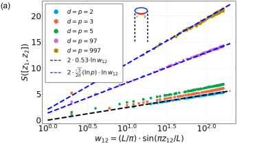
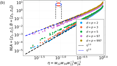
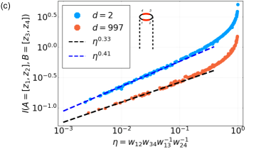
Figure 4: Numerical results for $d=p^{M=1}$. The fits for the critical exponents are summarized in Table 1. (a) We plot $S(A=[z_{1},z_{2}])$ against $\ln w_{12}$ (see Eq. (55)) at different values of $d=p$, where we see a clear dependence of the slope ($=2h_{a|b}$) on $p$. With increasing $p$, the value of $h_{a|b}$ approaches that of minimal cut percolation (see Eq. (53)). (b) The mutual negativity $N(A,B)$ between two disjoint subregions $A=[z_{1},z_{2}]$ and $B=[z_{3},z_{4}]$ against the cross ratio $\eta=(w_{12}w_{34})/(w_{13}w_{24})$. The powerlaw at small $\eta$ defines a critical exponent $h_{\rm MN}$, which has a clear dependence on $p$, and approaches minimal cut percolation at large $p$. (c) A “localizable entanglement” between $A$ and $B$. We perform a single-qudit projective measurements on each qudit outside $A\cup B$, and calculate the mutual information $I(A,B)$ subsequently. The powerlaw at small $\eta$ is another critical exponent $h_{f|f}^{(1)}$, which should in general take different values at different $p$, as we illustrate.

IV Numerical results

In this section we provide numerical evidence that supports our key conclusions from the previous sections on symmetry, namely that the universality class of the transition for qudit dimension $d=p^{M}$ depends on the prime number $p$, but not on the power $M$. To this end, we consider two cases:

(A) $d=p^{M}$ with fixed $M=1$ and different values of $p$, where we expect a series of different, $p$-dependent universality classes;

(B) $d=p^{M}$ with fixed $p$ and a few small values of $M$, where we expect to obtain the same exponents while varying $M$.

For each value of $d$, we simulate monitored Clifford circuits of $L=512$ qudits with periodic boundary condition, and focus on the steady state entanglement properties at their respective critical points. The circuit thus takes the geometry of a semi-infinite cylinder, and at criticality the entanglement entropy of a region $A$ is predicted to take the following form,

$$S(A=[z_{1},z_{2}])=2h_{a|b}\ln\left(\frac{L}{\pi}\sin\frac{\pi z_{12}}{L}\right)\coloneqq 2h_{a|b}\ln w_{12},$$ (55)

where $h_{a|b}$ is the scaling dimension of a (primary) boundary condition changing operator in the underlying CFT.

Data at the critical point	$d=2$	$d=3$	$d=5$	$d=97$	$d=997$
$p_{0,c}$	0.160	0.278	0.377	0.495	$0.500\approx 1/2$
$h_{a|b}$	0.53	0.62	0.66	$1.26\approx\frac{\sqrt{3}}{2\pi}\cdot\ln(97)$	$1.90\approx\frac{\sqrt{3}}{2\pi}\cdot\ln(997)$
$h_{\rm MN}$	3.0	2.9	2.6	2.2	2.0
$h_{f|f}^{(1)}$	0.41	-	-	-	$0.33\approx 1/3$

Table 1: A comparison of the location of the critical point $p_{0,c}$ and the operator scaling dimensions $h_{a|b},h_{\rm MN},h_{f|f}^{(1)}$ in hybrid Clifford circuits with different prime qudit dimensions $d=p$.

Data at the critical point	$d=2$	$d=3$	$d=5$	$d=23$	$d=503$
$h_{a|b}$	-	$0.53\approx 0.48\cdot\ln(3)$	$0.61\approx 0.38\cdot\ln(5)$	$0.91\approx 0.29\cdot\ln(23)$	$1.74\approx 0.28\cdot\ln(503)$
$h_{\rm MN}$	-	2.8	2.5	2.1	2.1
$h_{f|f}^{(1)}$	-	0.37	0.36	$0.33\approx 1/3$	$0.33\approx 1/3$

Table 2: Exponents for Clifford RTN Yang et al. (2021) with different prime qudit dimensions $d=p$. The exponents are all close to Clifford circuit, but different.

IV.1 Different universality classes at various $d=p^{M=1}$

Here, we take the qudit dimension to be a prime number, $d=p^{M=1}$ for $p\in\{2,3,5,97,997\}$. In Fig. 4(a), we plot the results of $S(A=[z_{1},z_{2}])$ in the form of Eq. (55), and extract the scaling dimension $h_{a|b}$ at the respective critical points. The locations of the critical points are determined by the best fit of $S(A=[z_{1},z_{2}])$ to a linear function of $\ln w_{12}$, see Eq. (55). The fits for $h_{a|b}$ and $p_{0,c}$ are collected in Table 1.

From our fitting, the scaling dimension $h_{a|b}$ clearly depends on $p$, and increases monotonically with $p$. It approaches the prediction from minimal cut percolation at large $p$, namely $h_{a|b}=\frac{\sqrt{3}}{2\pi}\ln p$ – see Eq. (53) and Eq. (55). In addition, the value of $p_{0,c}$ approaches $1/2$ as $p$ is increased, again consistent with bond percolation on a square lattice.

We also include results of the “mutual negativity” $N(A,B)$ between two disjoint regions $A=[z_{1},z_{2}]$ and $B=[z_{3},z_{4}]$ Sang et al. (2021). This quantity is expected to take the following form when the cross ratio $\eta$ for the four endpoints is small,

$$N(A=[z_{1},z_{2}],B=[z_{3},z_{4}])\propto\eta^{h_{\rm MN}},\text{ as }\eta\to 0.$$ (56)

Here, $h_{\rm MN}$ stands for the “mutual negativity exponent”. In Fig. 4(b) and Table 1, we see that $h_{\rm MN}$ is close to $3$ for smaller values of $d=p$, and approaches $2$ as $d=p$ becomes large, as consistent with minimal cut percolation Sang et al. (2021).

To further contrast universality classes at small $d=p$ with percolation at large $d=p$, we focus on the maximum and minimum qudit dimensions in our numerics, namely $d=p\in\{2,997\}$, and consider yet another quantity, known as a “localizable entanglement” Popp et al. (2005), recently introduced in the context of hybrid circuits Li et al. (2021). In this case, we again choose two disjoint regions $A=[z_{1},z_{2}]$ and $B=[z_{3},z_{4}]$, and perform a single-qudit projective measurement on each qudit outside $A\cup B$. In the post-measurement state, the mutual information between $A$ and $B$ is expected to be a conformal four-point function Li et al. (2021), and takes the following form when the cross ratio $\eta$ for the four endpoints is small,

$$I(A=[z_{1},z_{2}],B=[z_{3},z_{4}])\propto\eta^{h_{f|f}^{(1)}},\text{ as }\eta\to 0.$$ (57)

Here, $h_{f|f}^{(1)}$ is another critical exponent, which takes the value of $1/3$ in the percolation limit $d=p\to\infty$. In our numerics (see Fig. 4(c)), we find that $h_{f|f}^{(1)}$ fits well to $1/3\approx 0.33$ at $d=p=997$, but takes a distinct value $\approx 0.41$ at $d=p=2$ Li et al. (2021).

IV.2 Same universality class for $d=p$ and $d=p^{2}$

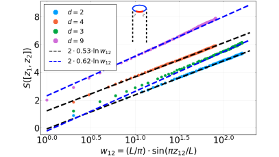
Figure 5: Numerical results for $d=p^{M}$, where we take $p\in\{2,3\}$ and $M\in\{1,2\}$. Comparing Fig. 4(a) and Eq. (55), we see that $h_{a|b}$ depends on the choice of $p$, but not on $M$.

Here we compare qudit dimensions $d=p^{M}$ at a fixed $p$ but different $M$. In order to probe the infrared fixed point, we choose $M=1,2$ so that $L\gg\xi(M)$, where $\xi(M)$ is a crossover length scale that diverges with $M$ (see Eq. (50)). Numerically accessing the crossover from $L\gg\xi(M)$ to $L\ll\xi(M)$ is an interesting problem left for future versions of this work.

For concreteness, we briefly describe the circuit model for $M>1$. At each site of the lattice we construct a “composite” qudit of dimension $d=p^{M}$ by grouping together $M$ “elementary” qudits each of dimension $p$. The circuit takes a brickwork architecture in the composite qudits, where nearest-neighbor composite qudits are coupled with random unitaries from the group $\mathrm{Cliff}(2M,p)$, and single composite qudits are subject to rank-1 projective measurements with probability $p_{0}$.

We compute the entanglement entropy $S(A)$ of region $A$ for $d\in\{2,4=2^{2}\}$ and for $d\in\{3,9=3^{2}\}$. The results are plotted in Fig. 5, where we see that $h_{a|b}$ depends $p$ but not on the choice of $M$. Results for $h_{a|b}$ at other values of $p$ also follow this pattern, but are not displayed.

Critical exponents for Clifford RTNs from Ref. Yang et al. (2021) are summarized in Table 2 for comparison. Somewhat surprisingly, numerical results indicate that the critical properties do not depend on the measurement scheme, forced (corresponding to the replica limit $Q\to 0$ in the statistical mechanics model) vs projective (replica limit $Q\to 1$) Yang et al. (2021), but appear to differ (slightly) between monitored Clifford circuits and Clifford RTNs for small $p$. Since the statistical mechanics models for RTNs (30) and monitored circuits (44) have the same symmetry group, we expect the entanglement transitions in both cases to be in the same universality class for a given measurement scheme (forced or projective). The numerical discrepancy between those cases might be due to strong corrections to scaling (i.e. from irrelevant operators) in the RTN case for small $p$, since there is no transition for $p=2$ in that case. One can, in principle, get an idea of the strength of such corrections by comparing Clifford RTNs with bond dimensions $d=p^{M}$ at a few small values of $M$, in a similar fashion to Fig. 5, although we leave a more thorough analysis of those corrections for future work.

V Discussion

In this work, we have introduced a replica statistical mechanics mapping to compute entanglement properties of stabilizer random tensor networks, and monitored Clifford quantum circuits acting on qudits with $d=p^{M}$. The degrees of freedom (‘spins’) of the resulting statistical models belong to the commutant of the Clifford group, using a generalization of the concept of Schur-Weyl duality to the Clifford case. We find that the Boltzmann weights are invariant under the left and right action of the stochastic orthogonal group with entries in the finite number field ${\bf F}_{p}$. This implies, suprisingly, that the universal properties of the entanglement transitions in Clifford circuits and RTNs depend on the on-site Hilbert space dimension $d$ but only through the prime $p$. This is in sharp constrast with the Haar case where the symmetry group is independent of $d$, as long as it is not infinite. Our formalism also allowed us to derive exact mappings onto classical percolation and minimal cut formulas as $d=p^{M}$ becomes large, with different consequences for $p$ fixed and $M\to\infty$, or $M$ fixed and $p\to\infty$. We confirmed our predictions using large scale stabilizer numerics.

Our results here bolster a known result about stabilizer tensors. Random stabilizer tensors with large bond dimension are perfect tensors with high probability Apel et al. (2021); Hayden et al. (2016); Pastawski et al. (2015). A perfect tensor has the special property of being a unitary gate for any equal-size bipartition of its legs. Thus, a Clifford circuit or RTN as $d\to\infty$ becomes an assembly of perfect tensors, for which the entanglement entropies are given exactly by the minimal cut through the underlying square lattice with randomly broken bonds.

Our approach could be generalized to other subgroups of the unitary group: formally, the main algebraic object that is needed would be the commutant of the subgroup. Once the commutant is known, most of the formulas derived in this manuscript carry over – including the definition of the Weingarten functions etc. It would be interesting to investigate whether other universality classes of entanglement transitions can be obtained in this way. As in the Haar case, an analytic understanding of the replica limit of the statistical mechanics models for finite $d$ remains a clear challenge for future work. One particularly intriguing aspect of our results is that while the statistical mechanics approach is certainly very powerful and allowed us to uncover the intricate dependence of the symmetry group on the prime number $p$, some aspects of Clifford circuits that are “simpler” (such as the ability to simulate them classically, or the flat entanglement spectrum of the reduced density matrix ) are not yet particularly transparent in the current formulation of our framework. Those special properties of the Clifford group might posssibly lead to some simplifications in the statistical mechanics formulation, that we leave for future work.

Appendix A Description and basic properties of the commutant $\Sigma_{Q}(p)$ for the Clifford case

The following statements (from Ref. Gross et al. (2021)) lead to the full characterization of the commutant $\Sigma_{Q}(p)$, which is presented in statement (iv) below, together with its properties relevant for the construction of the Clifford Stat. Mech. model, summarized in (v)-(vii):

-(i): (Stochastic) Orthogonal Group

For every $O\in{\cal O}_{Q}(p)$ the subspace

$$T_{O}:=\{(O\vec{\mu},\vec{\mu}):\ \ \vec{\mu}\in({\bf Z}_{p})^{Q}\}$$ (58)

is an element of $\Sigma_{Q}(p)$, and any operator ${\hat{r}}(T)$ as introduced in (23) is invertible if and only if $T$ is of the form $T=T_{O}$ for some $O\in{\cal O}_{Q}(p)$. Clearly, it follows from (23) that the operator ${\hat{r}}(T_{O})$ maps basis element $|\vec{\mu}\rangle$ into basis element $|O\vec{\mu}\rangle$. We will denote this operator simply by ${\hat{r}}(O)$, and we write simply ${\hat{r}}(T_{O})={\hat{r}}(O)$.

-(ii): Left and Right multiplication by (Stochastic) Orthogonal Group

For any subspace $T\in\Sigma_{Q}(p)$ as introduced in (23), and for any stochastic orthogonal matrix $O\in{\cal O}_{Q}(p)$, the objects

$$OT:=\{(O\vec{\nu},\vec{\mu}):\ (\nu,\mu)\in T\}$$ (59)

and

$$TO:=\{(\vec{\nu},O^{t}\vec{\mu}):\ (\nu,\mu)\in T\}$$

are themselves again elements of $\Sigma_{Q}(p)$, i.e. $OT,TO\in\Sigma_{Q}(p)$.

-(iii): Compatibility with ${\hat{r}}(T)$

The action with stochastic orthogonal matrices $O,O^{\prime}\in{\cal O}_{Q}(p)$ on subspaces $T\in\Sigma_{Q}(p)$, defined in (ii) above, translates naturally into the action on the corresponding operator ${\hat{r}}(T)$:

$${\hat{r}}(O){\hat{r}}(T){\hat{r}}(O^{\prime})=$$ (60)

$$={\hat{r}}(OT){\hat{r}}(O^{\prime})={\hat{r}}(O){\hat{r}}(TO^{\prime})={\hat{r}}(OTO^{\prime}).\qquad\qquad$$

-(iv): Double Coset Decomposition of Commutant

Statement (iii) above shows that the commutant $\Sigma_{Q}(p)$ is a disjoint union of double cosets with respect to the left- and right- actions of the stochastic orthogonal group, i.e.

$$\Sigma_{Q}(p)=$$ (61)

$$={\cal O}_{Q}(p)\ {\bar{T}}_{1}\ {\cal O}_{Q}(p)\ \cup\ ...\ \cup\ {\cal O}_{Q}(p)\ {\bar{T}}_{k}\ {\cal O}_{Q}(p),$$

where ${\bar{T}}_{1},...,{\bar{T}}_{k}$ denote representatives of different double cosets. It can be shown Gross et al. (2021) that $k\leq Q$. Here ${\bar{T}}_{1}=\Delta$ is the “diagonal subspace”

$$\Delta:=\{(\vec{\mu},\vec{\mu}):\ \ \vec{\mu}\in({\bf Z}_{p})^{Q}\},$$ (62)

so that ${\cal O}_{Q}(p)\ {\bar{T}}_{1}\ {\cal O}_{Q}(p)={\cal O}_{Q}(p)$.

-(v): Choice of representatives for Double Cosets

The operators ${\hat{r}}(T)$ associated with elements $T$ of the commutant that are not in the first double coset ${\cal O}_{Q}(p)\ {\bar{T}}_{1}\ {\cal O}_{Q}(p)={\cal O}_{Q}(p)$ are not invertible. Representatives ${\bar{T}}_{a}$ with $a=2,...,k$ can be chosen such that ${\hat{r}}({\bar{T}}_{a})$ are projectors. In particular, one can choose double coset representatives ${\bar{T}}_{a}$, $a=2,3,...,k$ (and the notation ${\bar{T}}_{a}$ denotes from now on that such a choice has been made) so that each is associated with a projector $P_{CSS(N_{a})}$ possessing a so-called ‘defect subspace’ $N_{a}\subseteq({\bf Z}_{p})^{Q}$ of dimension ${\rm dim}(N_{a})$, and

$${\hat{r}}({\bar{T}}_{a})=p^{{\rm dim}(N_{a})}P_{CSS(N_{a})},\quad(a=2,3,...,k)$$ (63)

with trace

$${\rm tr}\left[{\hat{r}}({\bar{T}}_{a})\right]=p^{Q-{\rm dim}(N_{a})}.$$ (64)

It is convenient to also introduce the notation ${\bar{T}}_{1}=\Delta$ and $N_{1}=0$.

-(vi): ‘Composition property’

Consider two arbitrary elements $T_{1},T_{2}\in\Sigma_{Q}(p)$ of the commutant. Each can then be reduced, upon right and left multiplication with elements in ${\cal O}_{Q}(p)$, to one of the elements ${\bar{T}}_{a}$, where $a=1,2,...,k$, and thus can be assigned a (possibly trivial) defect space $N_{a}$. Then the following composition property holds

$${\hat{r}}(T_{1}){\hat{r}}(T_{2})=p^{{\rm dim}(N_{1}\cap N_{2})}\ {\hat{r}}(T_{1}T_{2}).$$ (65)

-(vii): Trace

The commutant $\Sigma_{Q}(p)$ is equal to the disjoint union of sets $\Sigma_{Q}^{\ell}(p)$, where $\ell=0,1,...,(Q-1)$, whose elements are those elements $T\in\Sigma_{Q}(p)$ with the property that ${\rm dim}(T\cap\Delta)=Q-\ell$. Then, by the definition (23) of ${\hat{r}}(T)$ and the definition of the trace, one has

$${\rm tr}[{\hat{r}}(T)]=p^{Q-\ell},\quad{\rm for\ all\ elements}\ T\in\Sigma_{Q}^{\ell}(p).\qquad$$ (66)

-(viii): ‘Metric’ on an edge

For any two elements of the commutant $\Sigma_{Q}(p)$, in analogy with (20) in the Haar case, the Boltzmann weight on an edge of the Clifford RTN is built from

$${1\over p^{Q}}\ {\rm tr}\left(\left[{\hat{r}}(T_{1})\right]^{\dagger}{\hat{r}}(T_{2})\right)=\ e^{-\ln(p)\ |T_{1},T_{2}|}$$ (67)

where is $|T_{1},T_{2}|$ a metric defined by collecting (63,64, 65,66). It satisfies the usual conditions $|T_{1},T_{2}|=|T_{2},T_{1}|\geq 0$, and $|T_{1},T_{2}|=0$ if and only if $T_{1}=T_{2}$.

As a check, let us briefly compute the metric in the case where $T_{1}=T_{2}=T$, and thereby confirm that the above rules indeed yield the expected result $|T,T|=0$. There are two cases to consider. In the first case, $T\in{\cal O}_{Q}(p)$ is itself a group element, i.e. an element of the first double coset with ‘trivial’ representative $T_{1}=\Delta$. In this case the defect spaces are trivial (of dimension zero), and the trace in (67) is that of the identity operator acting on the (replicated) edge Hilbert space $({\bf C}^{p})^{Q}$, yielding $p^{Q}$. This is cancelled by the prefactor in (67) with the result that $|T,T|=0$ in this case, as expected. In the second case, $T$ is an element of one of the remaining (k-1) double cosets and is thus, upon right and left multiplication with possibly different group elements in ${\cal O}_{Q}(p)$, equal to one of the ‘projector’ representatives ${\bar{T}}_{a}$ with $a=2,...Q$. In this case ${\bar{T}}_{a}=$ $P_{CSS(N_{a})}$ is a projector satisfying $({\bar{T}}_{a})^{2}={\bar{T}}_{a}$, and (63,64, 65) yield for (67) the expression

$${1\over p^{Q}}\ p^{{\rm dim}(N_{a})}\ p^{Q-{\rm dim}(N_{a})}=1$$

in agreement with the expected result $|T,T|=0$.

-(ix): Symmetry of the ‘Metric’

It follows from its definition in (67) and from the compatibility property (60) that the metric $|T_{1},T_{2}|$ is invariant under the symmetry group ${\cal O}_{Q}(p)\times{\cal O}_{Q}(p)$, i.e. under right and left multiplication with arbitrary elements of the stochastic orthogonal group,

$$|T_{1},T_{2}|=|T^{\prime}_{1},T^{\prime}_{2}|,\ \ \ {\rm where}\ \ T_{1},T_{2}\in\Sigma_{Q}(p),$$ (68)

$${\rm and}$$

$$T^{\prime}_{1}=O_{L}T_{1}O_{R}^{-1},\ T^{\prime}_{2}=O_{L}T_{2}O_{R}^{-1},\ {\rm with}\ O_{L},O_{R}\in{\cal O}_{Q}(p)$$

Appendix B Basic properties of the Clifford Group, Stabilizer States, etc.

- (1) Single qudit ($d=p$=prime), Hilbert space ${\cal H}_{1}={\bf C}^{p}$, computational basis $|q\rangle$ with $q\in\{0,...,(p-1)\}={\bf Z}_{p}$. Pauli operators

$${\hat{X}}|q\rangle=|q+1\rangle,\quad{\hat{Z}}|q\rangle=\omega^{q}|q\rangle,\quad(\omega=e^{2\pi iq/d})$$

$${\hat{Y}}:=\tau{\hat{X}}^{\dagger}{\hat{Z}}^{\dagger},\quad({\rm where}\ \tau={\rm some\ suitable\ phase});$$

$${\rm Then:}\ \ {\hat{X}}{\hat{Y}}{\hat{Z}}=\tau{\bf I}$$ (69)

- (2) Hilbert space for $n$ qudits (d=p=prime) ${\cal H}_{n}=({\bf C}^{p})^{n}$, computational basis $|{\boldsymbol{q}}\rangle=$ $(q_{1},...,q_{n})\in({\bf Z}_{p})^{n}$.

- (3) Pauli Group ${\cal P}_{n}$ is the group generated by the tensor product of all Pauli operators on the $n$ qudits, or, equivalently, owing to (69), by the group generated by the tensor product of the operators $\tau{\hat{\bf I}},{\hat{X}},{\hat{Z}}$.

- (4) Clifford group ${\rm Cliff}(n,p)$ of the Hilbert space ${\cal H}_{n}=({\bf C}^{p})^{n}$ of $n$ qudits is the normalizer of the Pauli group in the unitary group acting on ${\cal H}_{n}=({\bf C}^{p})^{n}$, i.e. the group of all unitary operators ${\hat{V}}$ acting on ${\cal H}_{n}=({\bf C}^{p})^{n}$ satisfying ${\hat{V}}{\cal P}_{n}{\hat{V}}^{\dagger}\subset{\cal P}_{n}$, up to phases.

- (5) For a subgroup of the Pauli group, ${\cal S}\subset{\cal P}_{n}$ [one that does not contain any (non-trivial) multiple of the identity operator] the operator

$${\hat{\boldsymbol{P}}}_{\cal S}:={1\over|{\cal S}|}\sum_{{\hat{P}}\in{\cal S}}{\hat{P}},$$

is an orthogonal projector onto a subspace $V_{\cal S}\subset{\cal H}_{n}$ of dimension $p^{n}/|{\cal S}|$. When $|{\cal S}|=p^{n}$, the projection is onto a single state $|{\cal S}\rangle$ called a stabilizer state (i.e. $V_{\cal S}={\bf C}|{\cal S}\rangle$), which is thus the unique (up to scalars) eigenvector of all Pauli operators ${\hat{P}}$ in ${\cal S}$,

$${\hat{P}}|{\cal S}\rangle=|{\cal S}\rangle,\quad({\rm for\ all}\ {\hat{P}}\in{\cal S})$$

The (finite) set of all (pure) stabilizer states in ${\cal H}_{n}=({\bf C}^{p})^{n}$ is denoted by ${\rm Stab}(n,p)$. The number of stabilizer states Gross (2006) in ${\rm Stab}(n,p)$ is $=p^{n}\prod_{i=1}^{n}(p^{i}+1)$.

- (6) For every stabilizer state $|{\cal S}\rangle$ in ${\cal H}_{n}=({\bf C}^{p})^{n}$ there exists some Clifford unitary ${\hat{V}}\in{\rm Cliff}(n,p)$ such that

$$|{\cal S}\rangle={\hat{V}}\left(|0\rangle^{\otimes n}\right),\ \ [{\rm where}\ |0\rangle=|q=0\rangle,\ {\rm with}\ q=0\in{\bf F}_{p}].$$

It follows from this statement that the set of stabilizer states ${\rm Stab}(n,p)$ of the qudit Hilbert space ${\cal H}_{n}=({\bf C}^{p})^{n}$ is a single orbit of the action under the Clifford group ${\rm Cliff}(n,p)$.

- (7) There is a simple way to see that the state $|0\rangle^{\otimes n}\in{\cal H}_{n}=({\bf C}^{p})^{n}$, is a stabilizer state, i.e. an element of the set ${\rm Stab}(n,p)$ of stabilizer states.

The argument uses the notation of Weyl operators

$${\hat{W}}_{\bf x}={\hat{W}}_{\bf p,q}=\tau^{-{\bf p}\cdot{\bf q}}\left({\hat{Z}}^{p_{1}}{\hat{X}}^{q_{1}}\right)\otimes...\otimes\left({\hat{Z}}^{p_{n}}{\hat{X}}^{q_{n}}\right),$$

where ${\bf x}=({\bf p,q})\in{\cal V}_{n}:=({\bf Z}_{p})^{2n}$ (“phase space”). Each Weyl operator is an element of the Paul group ${\cal P}_{n}$; moreover, each element of the Pauli group is, up to a phase, equal to a Weyl operator. It is obvious [using (69)] that the state $|0\rangle^{\otimes n}\in{\cal H}_{n}$ is the simultaneous eigenvector of the set of all Weyl operators ${\hat{W}}_{\bf x}$ with ${\bf x}=({\bf p,q})$ where ${\bf q=0}$, i.e.

$${\hat{W}}_{\bf p,0}|0\rangle^{\otimes n}=|0\rangle^{\otimes n}.$$ (70)

This particular set of these Weyl operators thus represents the subgroup ${\cal S}\subset{\cal P}_{n}$ of the Pauli group, which “stablizes” the state $|0\rangle^{\otimes n}$. Note that the order of this subgroup of the Pauli group is $|{\cal S}|=p^{n}$, as required.

- (8) Futhermore, it is now possible to show that ${\hat{V}}|0\rangle^{\otimes n}$, where ${\hat{V}}\in{\rm Cliff}(n,p)$ is an arbitrary Clifford unitary operator in ${\cal H}_{n}$, is also a “stablilizer state”, i.e. an element of the set ${\rm Stab}(n,p)$ of stabilizer states. To see this, rewrite (70) as

$$\left({\hat{V}}{\hat{W}}_{\bf p,0}{\hat{V}}^{\dagger}\right)\ \left({\hat{V}}|0\rangle^{\otimes n}\right)=\left({\hat{V}}|0\rangle^{\otimes n}\right),$$

which says that the group of $p^{n}$ operators $\left({\hat{V}}{\hat{W}}_{\bf p,0}{\hat{V}}^{\dagger}\right)$ “stablizes” the state $\left({\hat{V}}|0\rangle^{\otimes n}\right)$. Owing to Eq. (2.8) of Gross et al. (2021) we know that

$${\hat{V}}{\hat{W}}_{\bf p,0}{\hat{V}}^{\dagger}=\omega^{f_{\hat{V}}({\bf p,0})}\ {\hat{W}}_{\Gamma_{\hat{V}}({\bf p,0})},$$

where $\Gamma_{\hat{V}}({\bf p,0})\in Sp(2n,p)$ and $f_{\hat{V}}({\bf x})$ is a suitable function on phase space ${\cal V}_{n}$ [defined under item (7) above - $Sp(2n,p)$ is the symplectic group with entries in the field ${\bf F}_{p}$.] Then since, as also mentioned under item (7) above, every Weyl operator is an element of the Pauli group, the group $\{{\hat{V}}{\hat{W}}_{\bf p,0}{\hat{V}}^{\dagger}:{\bf p}\in({\bf Z}_{p})^{n}\}$ forms a subgroup of the Pauli group ${\cal P}_{n}$ and can be identified with the “stabilizer” subgroup of the stablizer state ${\hat{V}}|0\rangle^{\otimes n}$.

- (9) Projective Clifford Group, Pauli Group, and orders of groups

Since we are interested in acting with elements of the Clifford group ${\hat{V}}\in{\rm Cliff}(n,p)$ on a density matrix of a pure state $|\psi\rangle$, i.e. ${\hat{V}}|\psi\rangle\ \langle\psi|{\hat{V}}^{\dagger}$, we can work with elements of the Clifford group modulo phases. We define the projective Clifford group as the Clifford group modulo phases, i.e. ${\overline{\rm Cliff}}(n,p):={\rm Cliff}(n,p)/U(1)$. Similarly, we call ${\overline{\cal P}}_{n}$ the Pauli group modulo phases. It can then be shown Gross et al. (2021); Gross (2006) that

$${\overline{\rm Cliff}}(n,p)/{\overline{\cal P}}_{n}={\rm Sp}_{2n}(p),$$

where, again, the latter is the symplectic group with entries in the field ${\bf F}_{p}$. Since the dimension of this symplectic group is known Gross (2006) to be $|{\rm Sp}_{2n}(p)|=$ $p^{n^{2}}\prod_{i=1}^{n}(p^{2i}-1)$, we know that the order of the projective Clifford group is

$$|{\overline{\rm Cliff}}(n,p)|=p^{2n}p^{n^{2}}\prod_{i=1}^{n}(p^{2i}-1),$$ (71)

where we used the fact (see item (7) above) that the projective Pauli Group is simply the set of all Weyl operators (of which there are as many as elements in “phase space” ${\cal V}_{n}$, defined above).

-(10) Average over the Clifford Group

It turns outGross et al. (2021) that, for an arbitrary (meaning: not a ‘stabilizer state’) state $|\psi\rangle\in{\cal H}_{n}$ the average

$$\sum_{{\hat{V}}\in{\rm Cliff}(n,p)}\left[{\hat{V}}|\psi\rangle\ \langle\psi|{\hat{V}}^{\dagger}\right]^{\otimes Q},$$ (72)

will, while still (obviously) expressible as a linear combination of the elements ${\hat{R}}(T)$ of the commutant, in general not simply be an equal-weight superposition of the latter, but may depend on details of the state $|\psi\rangle$ itself. However, if we take $|\psi\rangle$ to be any stabilizer state $|{\cal S}_{0}\rangle\in{\rm Stab}(n,p)\in{\cal H}_{n}$, the sum can be expressed as an equal-weight sum over the commutant, namely

$${1\over{\cal N}_{\rm norm}}\sum_{{\hat{V}}\in{\rm Cliff}(n,p)}\left[{\hat{V}}|{\cal S}_{0}\rangle\ \langle{\cal S}_{0}|{\hat{V}}^{\dagger}\right]^{\otimes Q}=$$ (73)

$$=\sum_{|{\cal S}\rangle\in{\rm Stab}(n,p)}\Big{[}|{\cal S}\rangle\ \langle{\cal S}|\Big{]}^{\otimes Q}={1\over Z_{n,p,Q}}\sum_{T\in\Sigma_{Q}(p)}{\hat{R}}(T),\qquad$$

where ${\cal N}_{\rm norm}$ and

$$Z_{n,p,Q}=p^{n}\prod_{k=1}^{(Q-2)}(p^{k}+p^{n}),$$

are normalization factors. The first equality follows because the set ${\rm Stab}(n,p)$ of stabilizer states is (see item (6) above) a single orbit under the action of the Clifford group on stabilizer states.

Appendix C Weingarten functions for Haar

Let us consider the operator (repeated indices summed)

$${\hat{X}}:=\mathbb{E}_{{\hat{U}}\in U(D)}\ \big{[}{\hat{U}}(...){\hat{U}}^{\dagger}\big{]}^{\otimes Q}=$$

$$=\int_{\rm Haar}d\mu({\hat{U}})\ \big{[}{\hat{U}}(...){\hat{U}}^{\dagger}\big{]}^{\otimes Q}=$$

$$=\int_{\rm Haar}d\mu(U)\ U_{\bar{i}_{1},j_{1}}...U_{\bar{i}_{Q},j_{Q}}U^{\dagger}_{\bar{j}_{1},i_{1}}...U^{\dagger}_{\bar{j}_{Q},i_{Q}}\times\qquad$$

$$\times\big{(}|\bar{i}_{1},...,\bar{i}_{Q}\rangle\langle i_{1},...,i_{Q}|\big{)}\otimes\big{(}|\bar{j}_{1},...,\bar{j}_{Q}\rangle\langle j_{1},...,j_{Q}|\big{)}$$

(74)

where $i_{1},...,\bar{i}_{Q},j_{1},...\bar{j}_{Q}\in\{1,...,D\}$. We can view the second tensor factor in the 4th line, $\big{(}|\bar{j}_{1},...,\bar{j}_{Q}\rangle\langle j_{1},...,j_{Q}|\big{)}$, as defining an orthonormal basis of the $Q$-fold tensor product of an “in” vector space of operators ${\cal H}^{\rm op}_{\rm in}$, i.e. of $\Big{(}{\cal H}^{\rm op}_{\rm in}\Big{)}^{\otimes Q}$. In the same way, we can view the first tensor factor in the 4th line, $\big{(}|\bar{i}_{1},...,\bar{i}_{Q}\rangle\langle i_{1},...,i_{Q}|\big{)}$, as defining an orthonormal basis of the $Q$-fold tensor product an “out” vector space of operators ${\cal H}^{\rm op}_{\rm out}$, i.e. of $\Big{(}{\cal H}^{\rm op}_{\rm out}\Big{)}^{\otimes Q}$. In other words, we can view ${\hat{X}}$ as an element of the tensor product of these two vector spaces of operators:

$${\hat{X}}\in\Big{(}{\cal H}^{\rm op}_{\rm out}\Big{)}^{\otimes Q}\otimes\Big{(}{\cal H}^{\rm op}_{\rm in}\Big{)}^{\otimes Q}.$$

Let us now consider a unitary operator ${\hat{W}}_{1}$ acting solely on ${\cal H}_{\rm out}$, while we act with the identity operator ${\bf I}$ on ${\cal H}_{\rm in}$. For such an operator we obtain

$$\Big{(}{{\hat{W}}_{1}}^{\otimes Q}\otimes{\bf I}^{\otimes Q}\Big{)}{\hat{X}}\Big{(}{{{\hat{W}}_{1}}^{\dagger\otimes Q}}\otimes{\bf I}^{\otimes Q}\Big{)}={\hat{X}}$$ (75)

which follows from the invariance of the Haar measure under left-multiplication of ${\hat{U}}$ with ${\hat{W}}_{1}$. Similarly, for a unitary operator ${\hat{W}}_{2}$ acting solely on ${\cal H}_{\rm in}$, while we act with the the identity operator on ${\cal H}_{\rm out}$, we obtain

$$\Big{(}{\bf I}^{\otimes Q}\otimes{{{\hat{W}}_{2}}^{\dagger\otimes Q}}\Big{)}{\hat{X}}\Big{(}{{\bf I}^{\otimes Q}\otimes{{\hat{W}}_{2}}}^{\otimes Q}\Big{)}={\hat{X}}$$ (76)

due to invariance of the Haar measure under right-multiplication of ${\hat{U}}$ by ${\hat{W}}_{2}$. Owing to (75) and (76), the operator ${\hat{X}}$ can be expanded as a tensor product of operators ${\hat{R}}(\sigma)$ which form a basis of the commutant acting on $\Big{(}{\cal H}^{\rm op}_{\rm in}\Big{)}^{\otimes Q}$, and operators ${\hat{R}}(\tau)$ which form a basis of the commutant acting on $\Big{(}{\cal H}^{\rm op}_{\rm out}\Big{)}^{\otimes Q}$, i.e.

$${\hat{X}}=\sum_{\sigma,\tau\in S_{Q}}\ \ \text{Wg}_{D}(\sigma,\tau)\ {\hat{R}}(\sigma)\otimes{\hat{R}}(\tau),$$ (77)

where $\text{Wg}_{D}(\sigma,\tau)$ are some coefficients called Weingarten functions. – Clearly, reading (74) in conjunction with (77), (17), and (18) is equivalent to the statement (10), and constitutes a proof of the latter.

We close this discussion with a slightly more compact, basis-independent formulation of the same facts. In particular, if we apply ${\hat{X}}$ to an operator in $\Big{(}{\cal H}^{\rm op}_{\rm in}\Big{)}^{\otimes Q}$ that is a $Q$-fold tensor product of an operator ${\hat{O}}_{\rm in}$ which is an element in the Hilbert space ${\cal H}^{\rm op}_{\rm in}$ of “in” operators, we obtain the following result which is an element of the $Q$-fold tensor product in the Hilbert space ${\cal H}^{\rm op}_{\rm out}$ of “out” operators:

$${\hat{X}}:\ \Big{(}{\cal H}^{\rm op}_{\rm in}\Big{)}^{\otimes Q} \to\Big{(}{\cal H}^{\rm op}_{\rm out}\Big{)}^{\otimes Q}$$

$$\left({\hat{O}}_{\rm in}\right)^{\otimes Q} \to{\hat{X}}\left[\left({\hat{O}}_{\rm in}\right)^{\otimes Q}\right]$$

where

$${\hat{X}}\left[\left({\hat{O}}_{\rm in}\right)^{\otimes Q}\right]=\int_{\rm Haar}d\mu({\hat{U}})\ \big{[}{\hat{U}}{\hat{O}}_{\rm in}{\hat{U}}^{\dagger}\big{]}^{\otimes Q}.$$

The operator ${\hat{X}}$ is (evidently) invariant under the action of independent unitary operators ${\hat{W}}_{1}$ and ${\hat{W}}_{2}$, implemented by right and left multiplication of the (integrated) Haar unitary ${\hat{U}}$

$${\hat{X}}\left[\left({\hat{O}}_{\rm in}\right)^{\otimes Q}\right]={\hat{X}}\left[{\hat{W}}_{2}^{\otimes Q}{\hat{O}}_{\rm in}^{\otimes Q}{{\hat{W}}_{2}^{\dagger\otimes Q}}\right]=$$

$$={\hat{W}}_{1}^{\otimes Q}\left({\hat{X}}\left[\left({\hat{O}}_{\rm in}\right)^{\otimes Q}\right]\right){{\hat{W}}_{1}^{\dagger\otimes Q}}.$$

This is the symmetry giving rise to the expansion (77) of ${\hat{X}}$ in terms of a tensor product of elements of the commutant. The same logic will apply in the Clifford case, the only difference being that the commutant will then be different.

We note for future use that we can apply the operator ${\hat{X}}$ to any element ${\hat{R}}(\tau)$ of the commutant, viewed as an element of the vector space of operators $\Big{(}{\cal H}^{\rm op}_{\rm in}\Big{)}^{\otimes Q}$. Using the fact that ${\hat{R}}(\tau)$ commutes by definition with ${\hat{U}}^{\otimes Q}$, we see that ${\hat{X}}\left[{\hat{R}}(\tau)\right]={\hat{R}}(\tau)$ where, by (C), the right hand side is an element of the vector space $\Big{(}{\cal H}^{\rm op}_{\rm out}\Big{)}^{\otimes Q}$.

C.1 Key properties of the Weingarten functions $\text{Wg}_{D}(\sigma,\tau)$ for the Haar case

Let us perform the trace over the second tensor factor $\Big{(}{\cal H}^{\rm op}_{\rm in}\Big{)}^{\otimes Q}$ of ${\hat{X}}$ defined in (74); we denote the trace over the 1st and 2nd tensor factor by ${\rm tr}^{(1)}$ and ${\rm tr}^{(2)}$. When denoting the identity operator in the first tensor factor, i.e. in ${\cal H}_{\rm out}$, by ${\bf I}$ we obtain for any permutation $\tau\in S_{Q}$

$${\rm tr}^{(2)}{\hat{X}}\left({\bf I}^{\otimes Q}\otimes{\hat{R}(\tau)}\right)={\hat{X}}\left[{\hat{R}}(\tau)\right]={\hat{R}}(\tau)=$$

$$=\sum_{\sigma_{o},\sigma_{i}\in S_{Q}}\ \ \text{Wg}_{D}(\sigma_{o},\sigma_{i})\ {\hat{R}}(\sigma_{o}){\rm tr}\left[{\hat{R}}^{\dagger}(\sigma_{i}){\hat{R}}(\tau)\right]=$$

$$=\sum_{\sigma_{o},\sigma_{i}\in S_{Q}}\ \ \text{Wg}_{D}(\sigma_{o},\sigma_{i})\ {\hat{R}}(\sigma_{o})\ D^{Q-|\sigma_{i},\tau|},$$ (79)

where in the first line we used the fact that ${\hat{R}}(\tau)$ is an element of the commutant [and the definition (74) of ${\hat{X}}$, as well as of the metric, (II.1) and (21)]; here $D=d^{2}$ is the dimension of the Hilbert space on which the 2-site unitary gate acts. Since ${\hat{R}}(\sigma_{o})$ form a basis of the commutant, (79) implies that

$$\sum_{\sigma_{i}}\text{Wg}_{D}(\sigma_{o},\sigma_{i})\ D^{Q-|\sigma_{i},\tau|}=\delta_{\sigma_{o},\tau}.$$ (80)

This equation says that the Weingarten function is the left-inverse of $D^{Q-|\sigma_{i},\tau|}$ under matrix multiplication when both are viewed as matrices.

The analogous argument applied to the equation ${\rm tr}^{(1)}{\hat{X}}\left({\hat{R}(\tau)\otimes{\bf I}^{\otimes Q}}\right)=$ ${\hat{R}}(\tau)$ implies a similar equation for the right inverse,

$$\sum_{\sigma_{o}}D^{Q-|\tau,\sigma_{o}|}\ \text{Wg}_{D}(\sigma_{o},\sigma_{i})=\delta_{\tau,\sigma_{i}}.$$ (81)

A simplification occurs in the Haar case because the metric satisfies $|\sigma,\tau|=$ $|\sigma^{-1}\tau|$, i.e. it doesn’t depend separately on $\sigma$ and $\tau$. This has two implications: (i) First, and most importantly, the Weingarten function, being the inverse of $D^{Q-|\sigma,\tau|}=$ $D^{Q-|\sigma^{-1}\tau|}$ is also a function of the combined variable, namely $\text{Wg}_{D}(\sigma_{o},\sigma_{i})=$ $\text{Wg}_{D}(\sigma^{-1}_{o}\sigma_{i})$. (ii) Second, without loss of generality, we may replace $\tau\to 1$ by the identity permutation $1$ in (80) and (81).

C.2 Consequences of (9) and (11)

Set $j_{1}=...=j_{Q}=\bar{j}_{1}=...=\bar{j}_{Q}=1$ in those equations. If we define the projection operator onto this state in $({\cal H}_{\rm in})^{\otimes Q}$,

$${\hat{\bf Q}^{0}}:={|1\rangle}^{\otimes Q}\ {\langle 1|}^{\otimes Q},$$

we conclude that

$${\rm tr}^{(2)}\big{[}{\hat{X}}\ \left({\bf I}^{\otimes Q}\otimes{\hat{\bf Q}^{0}}\right)\big{]}=$$

$$=\int_{\rm Haar}d\mu({\hat{U}})\ \big{[}{\hat{U}}|1\rangle\ {\langle 1|}{\hat{U}}^{\dagger}\big{]}^{\otimes Q}=$$

$$={\rm const.}\sum_{\tau\in S_{Q}}{\hat{R}}(\tau)$$

where we used (9), (11).

On the other hand, using the form (77) for ${\hat{X}}$, the same expression is equal to

$$=\sum_{\sigma,\tau\in S_{Q}}\ \ \text{Wg}_{D}(\sigma,\tau)\ {\hat{R}}(\sigma)\ \ \left({\rm tr}\big{[}{\hat{R}}(\tau)\ {\hat{\bf Q}^{0}}\big{]}\right)$$

Owing to (12) the trace in the above equation is unity independent of the element $\tau$ of the commutant $S_{Q}$,

$$\left({\rm tr}\big{[}{\hat{R}}(\tau)\ {\hat{\bf P}^{0}}\big{]}\right)=1,\quad{\rm for\ all}\ \tau\in S_{Q}.$$

We therefore conclude that

$${\rm const.}\sum_{\sigma\in S_{Q}}{\hat{R}}(\sigma)=$$

$$=\sum_{\sigma\in S_{Q}}\ \ \left(\sum_{\tau\in S_{Q}}\text{Wg}_{D}(\sigma,\tau)\right)\ {\hat{R}}(\sigma)$$

which means that the expression in parenthesis is a constant, independent of $\sigma$,

$$\sum_{\tau\in S_{Q}}\text{Wg}_{D}(\sigma,\tau)={\rm const.},\ \ {\rm for\ all}\ \sigma\in S_{Q}.\qquad\ \ \$$ (82)

Of course, here in the Weingarten case for Haar under consideration here, $\text{Wg}_{D}(\sigma,\tau)$ is a function of only $\sigma\tau^{-1}$ and so this condition is obviously satisfied.

Appendix D Weingarten functions for Clifford

Let us start with the analog of (74) for Clifford:

$${\hat{Y}}:=\mathbb{E}_{{\hat{V}}\in{\rm Cliff}(n,p)}\big{[}{\hat{V}}(...){\hat{V}}^{\dagger}\big{]}^{\otimes Q}=$$ (83)

$$={1\over{\cal N}_{\rm Cliff}}\sum_{{\hat{V}}\in{\rm Cliff}(n,p)}\ \big{[}{\hat{V}}(...){\hat{V}}^{\dagger}\big{]}^{\otimes Q}=$$

$$={1\over{\cal N}_{\rm Cliff}}\sum_{{\hat{V}}\in{\rm Cliff}(n,p)}V_{\bar{i}_{1},j_{1}}...V_{\bar{i}_{Q},j_{Q}}V^{\dagger}_{\bar{j}_{1},i_{1}}...V^{\dagger}_{\bar{j}_{Q},i_{Q}}\times\qquad$$

$$\times\big{(}|\bar{i}_{1},...,\bar{i}_{Q}\rangle\langle i_{1},...,i_{Q}|\big{)}\otimes\big{(}|\bar{j}_{1},...,\bar{j}_{Q}\rangle\langle j_{1},...,j_{Q}|\big{)},$$

$${\rm where}$$

$${\hat{Y}}\in\Big{(}{\cal H}^{\rm op}_{\rm out}\Big{)}^{\otimes Q}\otimes\Big{(}{\cal H}^{\rm op}_{\rm in}\Big{)}^{\otimes Q}.$$

Note that here $|i\rangle\in{\cal H}_{n}=({\bf C}_{p})^{n}$ is an orthonormal basis of ${\cal H}_{n}$, having no relationship with ‘stabilizer states’ in ${\cal H}_{n}$ (but see Sect. D.2 below). Now, the analogues of (75) and (76) follow upon the replacement ${\hat{X}}\to{\hat{Y}}$, for all Clifford unitary operators ${\hat{W}}_{1}$ and ${\hat{W}}_{2}$. Furthermore, the analog of (77) for the expansion of ${\hat{Y}}$ as a tensor product of operators in the commutant goes through in the same way as for Haar, leading to

$${\hat{Y}}=\sum_{T_{o},T_{i}\in\Sigma_{Q}(p)}\ \ \text{Wg}_{D}(T_{o},T_{i})\ {\hat{R}}(T_{o})\otimes{\hat{R}}(T_{i}),\qquad$$ (84)

where $\text{Wg}_{D}(T_{o},T_{i})$ are generalized Weingarten functions (see also Ref. Roth et al. (2018) for explicit expressions in the case of $Q=4$ replicas).

D.1 Key properties of the Weingarten functions $\text{Wg}_{D}(T_{o},T_{i})$ for the Clifford case

We proceed in complete analogy with the Haar case, discussed in Sect. C.1. For any element of the commutant $T\in\Sigma_{Q}(p)$, we have

$${\rm tr}^{(2)}{\hat{Y}}\left({\bf I}^{\otimes Q}\otimes{\hat{R}(T)}\right)={\hat{R}}(T)=$$

$$=\sum_{T_{o},T_{i}\in\Sigma_{Q}(p)}\ \ \text{Wg}_{D}(T_{o},T_{i})\ {\hat{R}}(T_{o}){\rm tr}\left[{\hat{R}}^{\dagger}(T_{i}){\hat{R}}(T)\right]=$$

$$=\sum_{T_{o},T_{i}\in\Sigma_{Q}(p)}\ \ \text{Wg}_{D}(T_{o},T_{i})\ {\hat{R}}(T_{o})D^{Q-|T_{i},T|},$$ (85)

where in the first line we used the fact that $T$ belongs to the commutant. We thus have

$$\sum_{T_{i}\in\Sigma_{Q}(p)}\ \ \text{Wg}_{D}(T_{o},T_{i})\ D^{Q-|T_{i},T|}=\delta_{T_{o},T}.$$ (86)

The last equation says that the Weingarten function is the left-inverse of $D^{Q-|T_{i},T|}$ (both viewed as a matrix). Similarly, by acting in the first line of (85) with ${\hat{R}}(T)$ on the first tensor factor and performing the trace over the first, we get a similar equation for the right-inverse.

D.2 Connection with Stabilizer States - consequences of (73)

To this end, we pick an orthonormal basis in $({\bf C}^{p})^{n}$ so that one element of this basis is the state $|0\rangle^{\otimes n}\in{\cal H}_{n}=({\bf C}^{p})^{n}$ where $0$ denotes the number zero in the finite number field ${\bf F}_{p}$; this is the state that is described in items (6) and (7) of Appendix B. Having done so, we use this orthonormal basis in (83) and set $j_{k}=j^{0}_{k}$, $\bar{j}_{k}=\bar{j^{0}}_{k}$ for $k=1,...,Q$, where $j^{0}_{1}=...=j^{0}_{Q}=\bar{j^{0}}_{1}=...=\bar{j^{0}}_{Q}=0^{\otimes n}$. (In better notation, $|j^{0}_{1}\rangle=...=|j^{0}_{Q}\rangle=$ $|0\rangle^{\otimes n}$, etc..)

If we define the projection operator onto this state in $({\cal H}_{\rm in})^{\otimes Q}$

$${\hat{\bf P}^{0}}:=\Big{[}{|0\rangle}^{\otimes n}\Big{]}^{\otimes Q}\ \ \ \Big{[}{\langle 0|}^{\otimes n}\Big{]}^{\otimes Q},$$

we conclude that

$${\rm tr}^{(2)}\big{[}{\hat{Y}}\ \left({\bf I}^{\otimes Q}\otimes{\hat{\bf P}^{0}}\right)\big{]}=$$

$$={1\over{\cal N}_{\rm Cliff}}\sum_{{\hat{V}}\in{\rm Cliff}(n,p)}\ \big{[}{\hat{V}}(|0\rangle^{\otimes n})\ \ ({\langle 0|}^{\otimes n}){\hat{V}}^{\dagger}\big{]}^{\otimes Q}=$$

$$={\rm const.}\sum_{T\in\Sigma_{Q}(p)}{\hat{R}}(T)$$

where we used (73).

On the other hand, using the form (84) for ${\hat{Y}}$, the same expression is equal to

$$=\sum_{T_{o},T_{i}\in\Sigma_{Q}(p)}\ \ \text{Wg}_{D}(T_{o},T_{i})\ {\hat{R}}(T_{o})\ \ \left({\rm tr}\big{[}{\hat{R}}(T_{i})\ {\hat{\bf P}^{0}}\big{]}\right).$$

Owing to Eq. (4.10) of Gross et al. (2021), the trace in the above equation is unity independent of the element $T_{i}$ of the commutant $\Sigma_{Q}(p)$,

$$\left({\rm tr}\big{[}{\hat{R}}(T_{i})\ {\hat{\bf P}^{0}}\big{]}\right)=1,\quad{\rm for\ all}\ T_{i}\in\Sigma_{Q}(p).$$

We therefore conclude that

$${\rm const.}\sum_{T\in\Sigma_{Q}(p)}{\hat{R}}(T)=$$

$$=\sum_{T_{o}\in\Sigma_{Q}(p)}\ \ \left(\sum_{T_{i}\in\Sigma_{Q}(p)}\text{Wg}_{D}(T_{o},T_{i})\right)\ {\hat{R}}(T_{o})$$

which means that the expresssion in parenthesis is a constant, independent of $T_{o}$,

$$\sum_{T_{i}\in\Sigma_{Q}(p)}\text{Wg}_{D}(T_{o},T_{i})={\rm const.},\ \ {\rm for\ all}\ T_{o}\in\Sigma_{Q}(p).\qquad\ \ \$$ (87)

This is the analog of (82) of the Haar case, where it is tied to the group structure of the commutant.

D.3 Generalization to other groups

Note that the generalized Weingarten formulas of the previous section do not rely on any specific property of the commutant of the Clifford group. As such, most of our results can be generalized to derive statistical mechanics models for RTNs and monitored quantum circuits involving averages over other subgroups of the unitary group, expressed in solely in terms of the commutant of such subgroups. Once this algebraic object, the commutant, is known, the link and Weingarten weights derived for the Clifford group carry over without any change, with the “spins” $T_{i}$ now belonging to this new commutant. Previously, Weingarten functions had been derived for unitary Collins (2003), orthogonal and symplectic groups Collins and Śniady (2006); Collins and Matsumoto (2009) — See Ref. Collins et al., 2021 for a recent review. The formulas in this appendix are completely general, and extend the notion of the Weingarten function to all situations for which the commutant is known.

References

- Amico et al. (2008) Luigi Amico, Rosario Fazio, Andreas Osterloh, and Vlatko Vedral, “Entanglement in many-body systems,” Rev. Mod. Phys. 80, 517–576 (2008).
- Horodecki et al. (2009) Ryszard Horodecki, Paweł Horodecki, Michał Horodecki, and Karol Horodecki, “Quantum entanglement,” Rev. Mod. Phys. 81, 865–942 (2009).
- Eisert et al. (2010) J. Eisert, M. Cramer, and M. B. Plenio, “Colloquium: Area laws for the entanglement entropy,” Rev. Mod. Phys. 82, 277–306 (2010).
- Calabrese and Cardy (2009) Pasquale Calabrese and John Cardy, “Entanglement entropy and conformal field theory,” Journal of Physics A: Mathematical and Theoretical 42, 504005 (2009).
- Laflorencie (2016) Nicolas Laflorencie, “Quantum entanglement in condensed matter systems,” Physics Reports 646, 1–59 (2016), quantum entanglement in condensed matter systems.
- Preskill (2018) John Preskill, “Quantum Computing in the NISQ era and beyond,” Quantum 2, 79 (2018).
- Nahum et al. (2017) Adam Nahum, Jonathan Ruhman, Sagar Vijay, and Jeongwan Haah, “Quantum entanglement growth under random unitary dynamics,” Phys. Rev. X 7, 031016 (2017).
- Nahum et al. (2018) Adam Nahum, Sagar Vijay, and Jeongwan Haah, “Operator Spreading in Random Unitary Circuits,” Physical Review X 8 (2018), 10.1103/PhysRevX.8.021014, arXiv:1705.08975 .
- von Keyserlingk et al. (2018) C. W. von Keyserlingk, Tibor Rakovszky, Frank Pollmann, and S. L. Sondhi, “Operator hydrodynamics, otocs, and entanglement growth in systems without conservation laws,” Phys. Rev. X 8, 021013 (2018).
- Zhou and Nahum (2019) Tianci Zhou and Adam Nahum, “Emergent statistical mechanics of entanglement in random unitary circuits,” Physical Review B 99 (2019), 10.1103/PhysRevB.99.174205, arXiv:1804.09737 .
- Rakovszky et al. (2018) Tibor Rakovszky, Frank Pollmann, and C. W. von Keyserlingk, “Diffusive hydrodynamics of out-of-time-ordered correlators with charge conservation,” Phys. Rev. X 8, 031058 (2018).
- Khemani et al. (2018) Vedika Khemani, Ashvin Vishwanath, and David A. Huse, “Operator spreading and the emergence of dissipative hydrodynamics under unitary evolution with conservation laws,” Phys. Rev. X 8, 031057 (2018).
- Li et al. (2018) Yaodong Li, Xiao Chen, and Matthew P. A. Fisher, “Quantum zeno effect and the many-body entanglement transition,” Phys. Rev. B 98, 205136 (2018).
- Skinner et al. (2019) Brian Skinner, Jonathan Ruhman, and Adam Nahum, “Measurement-Induced Phase Transitions in the Dynamics of Entanglement,” Physical Review X 9 (2019), 10.1103/PhysRevX.9.031009, arXiv:1808.05953 .
- Choi et al. (2020) Soonwon Choi, Yimu Bao, Xiao Liang Qi, and Ehud Altman, “Quantum Error Correction in Scrambling Dynamics and Measurement-Induced Phase Transition,” Physical Review Letters 125 (2020), 10.1103/PhysRevLett.125.030505, arXiv:1903.05124 .
- Gullans and Huse (2020a) Michael J. Gullans and David A. Huse, “Dynamical purification phase transition induced by quantum measurements,” Phys. Rev. X 10, 041020 (2020a).
- Li and Fisher (2021) Yaodong Li and Matthew P. A. Fisher, “Statistical mechanics of quantum error correcting codes,” Phys. Rev. B 103, 104306 (2021).
- Fan et al. (2021) Ruihua Fan, Sagar Vijay, Ashvin Vishwanath, and Yi-Zhuang You, “Self-organized error correction in random unitary circuits with measurement,” Phys. Rev. B 103, 174309 (2021).
- Li et al. (2019) Yaodong Li, Xiao Chen, and Matthew P.A. Fisher, “Measurement-driven entanglement transition in hybrid quantum circuits,” Physical Review B 100, 134306 (2019), arXiv:1901.08092 .
- Chan et al. (2019) Amos Chan, Rahul M. Nandkishore, Michael Pretko, and Graeme Smith, “Unitary-projective entanglement dynamics,” Phys. Rev. B 99, 224307 (2019).
- Li et al. (2021) Yaodong Li, Xiao Chen, Andreas W. W. Ludwig, and Matthew P. A. Fisher, “Conformal invariance and quantum nonlocality in critical hybrid circuits,” Phys. Rev. B 104, 104305 (2021).
- Cao et al. (2019) Xiangyu Cao, Antoine Tilloy, and Andrea De Luca, “Entanglement in a fermion chain under continuous monitoring,” SciPost Phys. 7, 24 (2019).
- Szyniszewski et al. (2019) M. Szyniszewski, A. Romito, and H. Schomerus, “Entanglement transition from variable-strength weak measurements,” Physical Review B 100 (2019), 10.1103/PhysRevB.100.064204, arXiv:1903.05452 .
- Bao et al. (2020) Yimu Bao, Soonwon Choi, and Ehud Altman, “Theory of the phase transition in random unitary circuits with measurements,” Physical Review B 101 (2020), 10.1103/PhysRevB.101.104301, arXiv:1908.04305 .
- Jian et al. (2020) Chao-Ming Jian, Yi-Zhuang You, Romain Vasseur, and Andreas W. W. Ludwig, “Measurement-induced criticality in random quantum circuits,” Phys. Rev. B 101, 104302 (2020).
- Gullans and Huse (2020b) Michael J. Gullans and David A. Huse, “Scalable Probes of Measurement-Induced Criticality,” Physical Review Letters 125 (2020b), 10.1103/PhysRevLett.125.070606, arXiv:1910.00020 .
- Zabalo et al. (2020) Aidan Zabalo, Michael J. Gullans, Justin H. Wilson, Sarang Gopalakrishnan, David A. Huse, and J. H. Pixley, “Critical properties of the measurement-induced transition in random quantum circuits,” Physical Review B 101 (2020), 10.1103/PhysRevB.101.060301, arXiv:1911.00008 .
- Nahum and Skinner (2020) Adam Nahum and Brian Skinner, “Entanglement and dynamics of diffusion-annihilation processes with majorana defects,” Phys. Rev. Research 2, 023288 (2020).
- Ippoliti et al. (2021) Matteo Ippoliti, Michael J. Gullans, Sarang Gopalakrishnan, David A. Huse, and Vedika Khemani, “Entanglement phase transitions in measurement-only dynamics,” Physical Review X 11 (2021), 10.1103/physrevx.11.011030.
- Lavasani et al. (2021) Ali Lavasani, Yahya Alavirad, and Maissam Barkeshli, “Measurement-induced topological entanglement transitions in symmetric random quantum circuits,” Nature Physics 17, 342–347 (2021).
- Sang and Hsieh (2021) Shengqi Sang and Timothy H. Hsieh, “Measurement-protected quantum phases,” Physical Review Research 3 (2021), 10.1103/physrevresearch.3.023200.
- Tang and Zhu (2020) Qicheng Tang and W. Zhu, “Measurement-induced phase transition: A case study in the nonintegrable model by density-matrix renormalization group calculations,” Phys. Rev. Research 2, 013022 (2020).
- Lopez-Piqueres et al. (2020) Javier Lopez-Piqueres, Brayden Ware, and Romain Vasseur, “Mean-field entanglement transitions in random tree tensor networks,” Phys. Rev. B 102, 064202 (2020).
- Nahum et al. (2021) Adam Nahum, Sthitadhi Roy, Brian Skinner, and Jonathan Ruhman, “Measurement and Entanglement Phase Transitions in All-To-All Quantum Circuits, on Quantum Trees, and in Landau-Ginsburg Theory,” PRX Quantum 2, 010352 (2021).
- Turkeshi et al. (2020) Xhek Turkeshi, Rosario Fazio, and Marcello Dalmonte, “Measurement-induced criticality in (2+1) -dimensional hybrid quantum circuits,” Physical Review B 102 (2020), 10.1103/PhysRevB.102.014315, arXiv:2007.02970 .
- Fuji and Ashida (2020) Yohei Fuji and Yuto Ashida, “Measurement-induced quantum criticality under continuous monitoring,” Phys. Rev. B 102, 054302 (2020).
- Lunt et al. (2021) Oliver Lunt, Marcin Szyniszewski, and Arijeet Pal, “Measurement-induced criticality and entanglement clusters: a study of 1d and 2d clifford circuits,” (2021), arXiv:2012.03857 [quant-ph] .
- Lunt and Pal (2020) Oliver Lunt and Arijeet Pal, “Measurement-induced entanglement transitions in many-body localized systems,” Phys. Rev. Research 2, 043072 (2020).
- Vijay (2020) Sagar Vijay, “Measurement-Driven Phase Transition within a Volume-Law Entangled Phase,” arXiv e-prints , arXiv:2005.03052 (2020), arXiv:2005.03052 [quant-ph] .
- Turkeshi et al. (2021) Xhek Turkeshi, Alberto Biella, Rosario Fazio, Marcello Dalmonte, and Marco Schiró, “Measurement-induced entanglement transitions in the quantum ising chain: From infinite to zero clicks,” Phys. Rev. B 103, 224210 (2021).
- Ippoliti and Khemani (2021) Matteo Ippoliti and Vedika Khemani, “Postselection-free entanglement dynamics via spacetime duality,” Phys. Rev. Lett. 126, 060501 (2021).
- Lu and Grover (2021) Tsung-Cheng Lu and Tarun Grover, “Entanglement transitions via space-time rotation of quantum circuits,” arXiv e-prints , arXiv:2103.06356 (2021), arXiv:2103.06356 [quant-ph] .
- Jian et al. (2020) Chao-Ming Jian, Bela Bauer, Anna Keselman, and Andreas W. W. Ludwig, “Criticality and entanglement in non-unitary quantum circuits and tensor networks of non-interacting fermions,” arXiv e-prints , arXiv:2012.04666 (2020), arXiv:2012.04666 [cond-mat.stat-mech] .
- Gopalakrishnan and Gullans (2021) Sarang Gopalakrishnan and Michael J. Gullans, “Entanglement and purification transitions in non-hermitian quantum mechanics,” Phys. Rev. Lett. 126, 170503 (2021).
- Turkeshi (2021) Xhek Turkeshi, “Measurement-induced criticality as a data-structure transition,” arXiv e-prints , arXiv:2101.06245 (2021), arXiv:2101.06245 [cond-mat.stat-mech] .
- Bao et al. (2021) Yimu Bao, Soonwon Choi, and Ehud Altman, “Symmetry enriched phases of quantum circuits,” arXiv e-prints , arXiv:2102.09164 (2021), arXiv:2102.09164 [cond-mat.stat-mech] .
- Block et al. (2021) Maxwell Block, Yimu Bao, Soonwon Choi, Ehud Altman, and Norman Yao, “The Measurement-induced Transition in Long-range Interacting Quantum Circuits,” arXiv e-prints , arXiv:2104.13372 (2021), arXiv:2104.13372 [quant-ph] .
- Bentsen et al. (2021) Gregory Bentsen, Subhayan Sahu, and Brian Swingle, “Measurement-induced purification in large-N hybrid Brownian circuits,” arXiv e-prints , arXiv:2104.07688 (2021), arXiv:2104.07688 [quant-ph] .
- Zabalo et al. (2021) Aidan Zabalo, Michael J. Gullans, Justin H. Wilson, Romain Vasseur, Andreas W. W. Ludwig, Sarang Gopalakrishnan, David A. Huse, and J. H. Pixley, “Operator scaling dimensions and multifractality at measurement-induced transitions,” arXiv e-prints , arXiv:2107.03393 (2021), arXiv:2107.03393 [cond-mat.dis-nn] .
- Agrawal et al. (2021) Utkarsh Agrawal, Aidan Zabalo, Kun Chen, Justin H. Wilson, Andrew C. Potter, J. H. Pixley, Sarang Gopalakrishnan, and Romain Vasseur, “Entanglement and charge-sharpening transitions in U(1) symmetric monitored quantum circuits,” arXiv e-prints , arXiv:2107.10279 (2021), arXiv:2107.10279 [cond-mat.dis-nn] .
- Li and Fisher (2021) Yaodong Li and Matthew P. A. Fisher, “Robust decoding in monitored dynamics of open quantum systems with Z_2 symmetry,” arXiv e-prints , arXiv:2108.04274 (2021), arXiv:2108.04274 [quant-ph] .
- Alberton et al. (2021) O. Alberton, M. Buchhold, and S. Diehl, “Entanglement transition in a monitored free-fermion chain: From extended criticality to area law,” Phys. Rev. Lett. 126, 170602 (2021).
- Jian et al. (2021) Shao-Kai Jian, Chunxiao Liu, Xiao Chen, Brian Swingle, and Pengfei Zhang, “Quantum error as an emergent magnetic field,” arXiv e-prints , arXiv:2106.09635 (2021), arXiv:2106.09635 [quant-ph] .
- Lunt et al. (2020) Oliver Lunt, Marcin Szyniszewski, and Arijeet Pal, “Measurement-induced criticality and entanglement clusters: a study of 1D and 2D Clifford circuits,” arXiv e-prints , arXiv:2012.03857 (2020), arXiv:2012.03857 [quant-ph] .
- Buchhold et al. (2021) M. Buchhold, Y. Minoguchi, A. Altland, and S. Diehl, “Effective Theory for the Measurement-Induced Phase Transition of Dirac Fermions,” arXiv e-prints , arXiv:2102.08381 (2021), arXiv:2102.08381 [cond-mat.stat-mech] .
- Noel et al. (2021) Crystal Noel, Pradeep Niroula, Daiwei Zhu, Andrew Risinger, Laird Egan, Debopriyo Biswas, Marko Cetina, Alexey V. Gorshkov, Michael J. Gullans, David A. Huse, and Christopher Monroe, “Observation of measurement-induced quantum phases in a trapped-ion quantum computer,” arXiv e-prints , arXiv:2106.05881 (2021), arXiv:2106.05881 [quant-ph] .
- Vasseur et al. (2019) Romain Vasseur, Andrew C. Potter, Yi-Zhuang You, and Andreas W. W. Ludwig, “Entanglement transitions from holographic random tensor networks,” Phys. Rev. B 100, 134203 (2019).
- Levy and Clark (2021) Ryan Levy and Bryan K. Clark, “Entanglement Entropy Transitions with Random Tensor Networks,” arXiv e-prints , arXiv:2108.02225 (2021), arXiv:2108.02225 [cond-mat.stat-mech] .
- Yang et al. (2021) Zhi-Cheng Yang, Yaodong Li, Matthew P. A. Fisher, and Xiao Chen, “Entanglement phase transitions in random stabilizer tensor networks,” (2021), arXiv:2107.12376 [cond-mat.stat-mech] .
- Hayden et al. (2016) Patrick Hayden, Sepehr Nezami, Xiao-Liang Qi, Nathaniel Thomas, Michael Walter, and Zhao Yang, “Holographic duality from random tensor networks,” Journal of High Energy Physics 2016, 9 (2016).
- Nezami and Walter (2020) Sepehr Nezami and Michael Walter, “Multipartite entanglement in stabilizer tensor networks,” Phys. Rev. Lett. 125, 241602 (2020).
- Gottesman (1996) Daniel Gottesman, “Class of quantum error-correcting codes saturating the quantum hamming bound,” Phys. Rev. A 54, 1862–1868 (1996).
- Gottesman (1998) Daniel Gottesman, “The Heisenberg Representation of Quantum Computers,” arXiv e-prints , quant-ph/9807006 (1998), arXiv:quant-ph/9807006 [quant-ph] .
- Aaronson and Gottesman (2004) Scott Aaronson and Daniel Gottesman, “Improved simulation of stabilizer circuits,” Phys. Rev. A 70, 052328 (2004).
- Chandran and Laumann (2015) Anushya Chandran and C. R. Laumann, “Semiclassical limit for the many-body localization transition,” Phys. Rev. B 92, 024301 (2015).
- Gross et al. (2021) David Gross, Sepehr Nezami, and Michael Walter, “Schur–weyl duality for the clifford group with applications: Property testing, a robust hudson theorem, and de finetti representations,” Communications in Mathematical Physics 385, 1325–1393 (2021).
- Gottesman (1999) Daniel Gottesman, “Fault-Tolerant Quantum Computation with Higher-Dimensional Systems,” Chaos Solitons and Fractals 10, 1749–1758 (1999), arXiv:quant-ph/9802007 [quant-ph] .
- Collins (2003) Benoît Collins, “Moments and cumulants of polynomial random variables on unitarygroups, the Itzykson-Zuber integral, and free probability,” International Mathematics Research Notices 2003, 953–982 (2003), https://academic.oup.com/imrn/article-pdf/2003/17/953/1881428/2003-17-953.pdf .
- Chayes et al. (1986) J. T. Chayes, L. Chayes, and R. Durrett, “Critical behavior of the two-dimensional first passage time,” Journal of Statistical Physics 45, 933–951 (1986).
- Jiang and Yao (2016) Jianping Jiang and Chang-Long Yao, “Critical first-passage percolation starting on the boundary,” arXiv e-prints , arXiv:1612.01803 (2016), arXiv:1612.01803 [math.PR] .
- Sang et al. (2021) Shengqi Sang, Yaodong Li, Tianci Zhou, Xiao Chen, Timothy H. Hsieh, and Matthew P.A. Fisher, “Entanglement negativity at measurement-induced criticality,” PRX Quantum 2, 030313 (2021).
- Popp et al. (2005) M. Popp, F. Verstraete, M. A. Martín-Delgado, and J. I. Cirac, “Localizable entanglement,” Phys. Rev. A 71, 042306 (2005), arXiv:quant-ph/0411123 [quant-ph] .
- Apel et al. (2021) Harriet Apel, Tamara Kohler, and Toby Cubitt, “Holographic duality between local hamiltonians from random tensor networks,” (2021), arXiv:2105.12067 [hep-th] .
- Pastawski et al. (2015) Fernando Pastawski, Beni Yoshida, Daniel Harlow, and John Preskill, “Holographic quantum error-correcting codes: toy models for the bulk/boundary correspondence,” Journal of High Energy Physics 2015 (2015), 10.1007/jhep06(2015)149.
- Calderbank and Shor (1996) A. R. Calderbank and Peter W. Shor, “Good quantum error-correcting codes exist,” Phys. Rev. A 54, 1098–1105 (1996), arXiv:quant-ph/9512032 [quant-ph] .
- Steane (1996) Andrew Steane, “Multiple-Particle Interference and Quantum Error Correction,” Proceedings of the Royal Society of London Series A 452, 2551–2577 (1996), arXiv:quant-ph/9601029 [quant-ph] .
- Steane (1996) A. M. Steane, “Error correcting codes in quantum theory,” Phys. Rev. Lett. 77, 793–797 (1996).
- Gross (2006) D. Gross, “Hudson’s theorem for finite-dimensional quantum systems,” Journal of Mathematical Physics 47, 122107 (2006), https://doi.org/10.1063/1.2393152 .
- Roth et al. (2018) I. Roth, R. Kueng, S. Kimmel, Y.-K. Liu, D. Gross, J. Eisert, and M. Kliesch, “Recovering quantum gates from few average gate fidelities,” Phys. Rev. Lett. 121, 170502 (2018).
- Collins and Śniady (2006) Benoît Collins and Piotr Śniady, “Integration with respect to the haar measure on unitary, orthogonal and symplectic group,” Communications in Mathematical Physics 264, 773–795 (2006).
- Collins and Matsumoto (2009) Benoît Collins and Sho Matsumoto, “On some properties of orthogonal weingarten functions,” Journal of Mathematical Physics 50, 113516 (2009), https://doi.org/10.1063/1.3251304 .
- Collins et al. (2021) Benoit Collins, Sho Matsumoto, and Jonathan Novak, “The Weingarten Calculus,” arXiv e-prints , arXiv:2109.14890 (2021), arXiv:2109.14890 [math-ph] .