Continuous logistic Gaussian random measure fields for spatial distributional modelling

Abstract

We investigate a class of models for non-parametric estimation of probability density fields based on scattered samples of heterogeneous sizes. The considered SLGP models are Spatial extensions of Logistic Gaussian Process models and inherit some of their theoretical properties but also of their computational challenges. We introduce SLGPs from the perspective of random measures and their densities, and investigate links between properties of SLGPs and underlying processes. Our inquiries are motivated by SLGP’s abilities to deliver probabilistic predictions of conditional distributions at candidate points, to allow (approximate) conditional simulations of probability densities, and to jointly predict multiple functionals of target distributions. We show that SLGP models induced by continuous GPs can be characterized by the joint Gaussianity of their log-increments and leverage this characterization to establish theoretical results pertaining to spatial regularity. We extend the notion of mean-square continuity to random measure fields and establish sufficient conditions on covariance kernels underlying SLGPs for associated models to enjoy such regularity properties. From the practical side, we propose an implementation relying on Random Fourier Features and demonstrate its applicability on synthetic examples and on temperature distributions at meteorological stations, including probabilistic predictions of densities at left-out stations.

, and

1 Introduction

1.1 Motivations and context

One of the central problems in statistics and stochastic modelling is to capture and encode the dependence of a random response on predictors in a flexible manner. Estimating some (conditional) response distributions given values of predictors $\mathbf{x}=(x_{1},...,x_{d})$ is sometimes referred to as density regression and has received attention in many scientific application areas. However, this problem becomes particularly challenging when this dependence does not only concern the mean and/or the variance of the distribution, but other features can evolve, including for instance their shape, their uni-modal versus multi-modal nature, etc. An example of temperature distribution field is represented in Fig. 1.

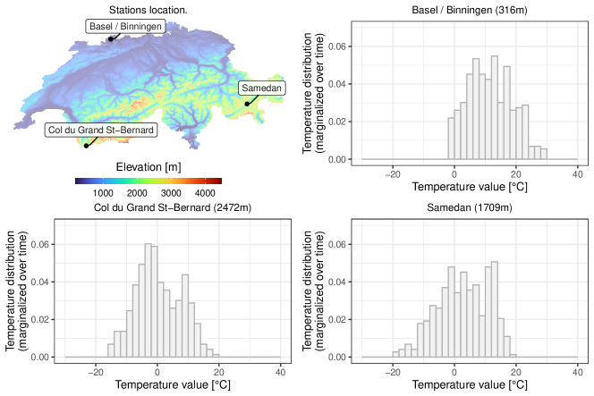
Figure 1: One example of probability distribution field: The daily mean temperatures in Switzerland indexed by latitude, longitude and altitude. We display the histogram of the available data for three meteorological stations (365 replications for each location).

Among the most notable approaches typically used in a frequentist framework to address this challenge, one can cite finite mixture models [39] or kernel density estimation [12, 19]. Kernel approaches usually require estimating the bandwidth which is done with cross-validation [13], bootstrap [19] or other methods. Generalized lambda distributions have recently been used in [49] for flexible semi-parametric modelling of unimodal distributions depending on covariables.

Within a Bayesian context, it is natural to put a prior on probability density functions and derive posterior distributions of such probability density functions given observed data. The most common class of models are infinite mixture models. Its popularity is partly due to the wide literature on algorithms for posterior sampling within a Markov Chain Monte Carlo framework [21, 48, 33] or fast approximation [29]. Non-parametric approaches include generalizing stick breaking processes [10, 11, 5, 17], multivariate transformation of a Beta distribution [46] or transforming a Gaussian Process (GP) [22, 8, 45, 15]. The Spatial Logistic Gaussian Process (SLGP) model, related to [45] and being at the center of the present contribution following up on [15], is itself a spatial generalization of the Logistic Gaussian Process (LGP) model.

The LGP for density estimation was established and studied in [25, 26, 27] and is commonly introduced as a random probability density function obtained by applying a non-linear transformation (or “mapping”) $\psi$ to a sufficiently well-behaved GP $Z=(Z_{t})_{t\in\mathcal{T}}$, resulting in

$$\psi[Z](t)=\frac{e^{Z_{t}}}{\int_{\mathcal{T}}e^{Z_{u}}\,d\lambda(u)}\text{ for all }t\in\mathcal{T}$$ (1)

Here and throughout the document, we consider a compact and convex response space $\mathcal{T}\subset\mathbb{R}^{d_{\mathcal{T}}}$ with $d_{\mathcal{T}}\geq 1$ and we denote by $\lambda$ the Lebesgue measure on $\mathbb{R}^{d_{\mathcal{T}}}$. We further assume that $\lambda(\mathcal{T})>0$.

For the Spatial Logistic Gaussian Process (SLGP), we will similarly build upon a well-behaved GP $(Z_{\mathbf{x},t})_{(\mathbf{x},t)\in D\times\mathcal{T}}$ (now indexed by a product set) and study the stochastic process obtained from applying spatial logistic transformation to $Z$ as follows:

$$\Psi[Z](\mathbf{x},t)=\dfrac{e^{Z_{\mathbf{x},t}}}{\int_{\mathcal{T}}e^{Z_{\mathbf{x},u}}\,d\lambda(u)}\text{ for all }(\mathbf{x},t)\in D\times\mathcal{T}$$ (2)

where $D\subset\mathbb{R}^{d_{D}}$ is a compact and convex index space with $d_{D}\geq 1$.

At any fixed $\mathbf{x}$, $\Psi[Z](\mathbf{x},\cdot)$ hence returns an LGP, so that an SLGP can be seen as a field of LGPs. What the mathematical objects involved precisely are (in terms of random measures or densities, and fields thereof) calls for some careful analysis, underlying the first question that we will focus on in the present article:

Question 1: What (kind of stochastic models) are (S)LGPs?

We revisit both LGP and SLGP models in terms of random measures and random measure fields, investigating in turn different notions of equivalence and indistinguishability between random measure fields. Also, since finite-dimensional distributions of Gaussian Processes are characterized by mean and covariance functions, it can be tempting to jump to the conclusion that the latter functions characterize SLGPs. As we show here, things are in fact not so simple, due in the first place to the fact that SLGPs require to control measurability and further properties of GPs beyond finite-dimensional distributions, but also because $\psi$ is invariant under translations of $Z$ by constants (resp. $\Psi$ is invariant under translations of $Z$ by functions of $\mathbf{x}$). We go on with asking what characterizes SLGPs among fields of random measures with prescribed positivity properties:

Question 2: Given a random field of positive densities, how to characterize that it is an SLGP and what can then be said about the underlying GP(s)?

Thereby we keep a particular interest for the role of covariance kernels. We denote here and in the following by $k$ the covariance kernel of $Z$.

In geostatistics and spatial statistics [28, 42, 7], quantifying the spatial regularity of scalar valued (Gaussian) processes such as $Z$ (with links to properties of $k$ in centered squared integrable cases) have been well studied and a wide literature is available. Similar approaches have been investigated in settings of function valued processes [38, 20, 30] but the main contributions in such cases are generally limited to stationary functional stochastic processes valued in $L^{2}$. Extensions to the distributional setting have also been proposed through embedding into an infinite-dimensional Hilbert Space using Aitchison geometry [1, 35] and classical results on stationary functional processes. Here, we tackle notions of spatial regularity between (random) measures / probability densities that does not require Hilbert Space embedding. More specifically, we focus on:

Question 3: How to quantify spatial regularity in (LG) random measure fields?

For that we investigate generalizations of scalar-valued continuity notions (mean-square continuity and almost sure continuity) in the context of random measure fields, and especially of SLGPs. This leads us to our ultimate question, naturally following as an extension of results from the scalar valued case to (selected cases of) SLGPs:

Question 4: To what extent is the spatial regularity of SLGPs driven by k?

Sufficient conditions of mean-power continuity (with respect to the Total Variation and Hellinger distances, as well as to the Kullback-Leibler divergence) of SLGPs are established in terms of the covariance kernel of a suitable field of log-increment underlying the considered SLGPs. Also, almost sure results are obtained, that build upon general results on Gaussian measures in Banach spaces.

This document is structured in the following way: in Section 2, we mostly focus on Questions $1$ and $2$ by revisiting LGPs in terms of Random Probability Measures and extending this construction to SLGPs by introducing Random Probability Measure Fields (RPMFs). In particular, we establish the following result:

Proposition 2.6.

For any two measurable RFs $Z:=(Z_{\mathbf{x},t})_{(\mathbf{x},t)\in D\times\mathcal{T}}$ and $\tilde{Z}:=(\tilde{Z}_{\mathbf{x},t})_{(\mathbf{x},t)\in D\times\mathcal{T}}$ such that $\int_{\mathcal{T}}e^{Z_{\mathbf{x},u}(\omega)}\,d\lambda(u)<\infty$ and $\int_{\mathcal{T}}e^{\tilde{Z}_{\mathbf{x},u}(\omega)}\,d\lambda(u)<\infty$ for any $(\mathbf{x},\omega)\in D\times\Omega$, we have:

1. $\left(Z_{\mathbf{x},t}-Z_{\mathbf{x},t^{\prime}}\right)_{(\mathbf{x},t,t^{\prime})\in D\times\mathcal{T}^{2}}$ and $\left(\tilde{Z}_{\mathbf{x},t}-\tilde{Z}_{\mathbf{x},t^{\prime}}\right)_{(\mathbf{x},t,t^{\prime})\in D\times\mathcal{T}^{2}}$ are indistinguishable from one-another.

2. $\left(\frac{e^{Z_{\mathbf{x},t}}}{\int_{\mathcal{T}}e^{Z_{\mathbf{x},u}}\,d\lambda(u)}\right)_{(\mathbf{x},t)\in D\times\mathcal{T}}$ is indistinguishable from $\left(\frac{e^{\tilde{Z}_{\mathbf{x},t}}}{\int_{\mathcal{T}}e^{\tilde{Z}_{\mathbf{x},u}}\,d\lambda(u)}\right)_{(\mathbf{x},t)\in D\times\mathcal{T}}$.

3. $\left(\frac{\int_{B}e^{Z_{\mathbf{x},u}}\,d\lambda(u)}{\int_{\mathcal{T}}e^{Z_{\mathbf{x},u}}\,d\lambda(u)}\right)_{(B,\mathbf{x})\in\mathcal{B}(\mathcal{T})\times D}$ is indistinguishable from $\left(\frac{\int_{B}e^{\tilde{Z}_{\mathbf{x},u}}\,d\lambda(u)}{\int_{\mathcal{T}}e^{\tilde{Z}_{\mathbf{x},u}}\,d\lambda(u)}\right)_{(B,\mathbf{x})\in\mathcal{B}(\mathcal{T})\times D}$.

Additionally, if $Z$ and $\tilde{Z}$ are almost surely continuous, $(3)\Rightarrow(2)$.

Proposition 2.10.

Let us consider a measurable, separable GP $Z=(Z_{\mathbf{x},t})_{(\mathbf{x},t)\in D\times\mathcal{T}}$ that is almost-surely continuous in $t$, and such that $\int_{\mathcal{T}}e^{Z_{\mathbf{x},u}(\omega)}\,d\lambda(u)<\infty$ for any $(\mathbf{x},\omega)\in D\times\Omega$. Then, for any $\mathbf{x}\in D$, $\Psi[Z](\mathbf{x},\cdot)$ is almost surely the continuous representer of the Radon-Nikodym derivative of $B\in\mathcal{B}(\mathcal{T})\mapsto\frac{\int_{B}e^{Z_{\mathbf{x},u}}\,d\lambda(u)}{\int_{\mathcal{T}}e^{Z_{\mathbf{x},u}}\,d\lambda(u)}$.

Throughout Section 3, we study the spatial regularity of the SLGP by relying on notions in spatial statistics and basic yet powerful results from Gaussian measure theory. Assuming that our SLGP is obtained by transforming $Z\sim\mathcal{GP}(0,k)$, we do so by leveraging the following condition on $k$:

Condition 2.

There exist $C,\alpha_{1},\alpha_{2}>0$ such that for all $\mathbf{x},\mathbf{x}^{\prime}\in D,t,t^{\prime}\in\mathcal{T}$:

$$k([\mathbf{x},t],[\mathbf{x},t])+k([\mathbf{x}^{\prime},t^{\prime}],[\mathbf{x}^{\prime},t^{\prime}])-2k([\mathbf{x},t],[\mathbf{x}^{\prime},t^{\prime}])\leq C\cdot\max(\|\mathbf{x}-\mathbf{x}^{\prime}\|_{\infty}^{\alpha_{1}},\|t-t^{\prime}\|_{\infty}^{\alpha_{2}})$$

Theorem 3.6.

Let us consider a centred GP $Z$ on $D\times\mathcal{T}$ whose covariance kernel $k$ satisfies Condition 2. The SLGP induced by $Z$ denoted here $Y$ is almost surely a positive pdf field and it is almost surely $\beta$-Hölder continuous with respect to $\|\cdot\|_{\infty}$, for any $\beta<\frac{\alpha_{1}}{2}$.

Theorem 3.7 .

Consider the SLGP $Y$ induced by a centred GP $Z$ with covariance kernel $k$ and assume that $k$ satisfies Condition 2.

Then, for all $\gamma>0$ and $0<\delta<\gamma\alpha_{1}/2$ (for Equation 3, resp. $0<\delta<\gamma\alpha_{1}$ for Equations 4 and 5), there exists $K_{\gamma,\delta}>0$ such that for all $\mathbf{x},\mathbf{x}^{\prime}\in D^{2}$:

$$\mathbb{E}\left[d_{H}(Y_{\mathbf{x},\cdot},Y_{\mathbf{x}^{\prime},\cdot})^{\gamma}\right]\leq K_{\gamma,\delta}\|\mathbf{x}-\mathbf{x}^{\prime}\|^{\gamma\alpha_{1}/2-\delta}_{\infty}$$ (3)

$$\mathbb{E}\left[KL(Y_{\mathbf{x},\cdot},Y_{\mathbf{x}^{\prime},\cdot})^{\gamma}\right]\leq K_{\gamma,\delta}\|\mathbf{x}-\mathbf{x}^{\prime}\|^{\gamma\alpha_{1}-\delta}_{\infty}$$ (4)

$$\mathbb{E}\left[d_{TV}(Y_{\mathbf{x},\cdot},Y_{\mathbf{x}^{\prime},\cdot})^{\gamma}\right]\leq K_{\gamma,\delta}\|\mathbf{x}-\mathbf{x}^{\prime}\|^{\gamma\alpha_{1}-\delta}_{\infty}$$ (5)

Some results over analytical test functions and a test case are presented in Section 4. From the computational side, we introduce a Markov Chain Monte Carlo algorithmic approach for conditional density estimation relying on Random Fourier Features approximation [36, 37], and apply it to a meteorological data set. We also included in Appendix: definitions and properties of the notion of consistency as well as some short results of posterior consistency (D), some proofs (C) and details on the implementation of the density field estimation (E).

1.2 Further notations and working assumptions

Throughout the article, we denote by $(\Omega,\mathcal{F},P)$ the ambient probability space. We will also denote by $\mathcal{B}(\mathcal{T})$ the Borel $\sigma$-algebra induced by the Euclidean metric on $\mathcal{T}$. For a set $S$ (here $\mathcal{T}$ or $D\times\mathcal{T}$), we denote by $\mathcal{C}^{0}(S)$, $\mathcal{A}(S)$, $\mathcal{A}^{+}(S)$ the sets of continuous real functions, Probability Density Functions (PDFs) and almost everywhere positive PDFs on $S$, respectively. Finally, we denote by $\mathcal{A}(D;\mathcal{T})$ the set of fields of PDFs on $\mathcal{T}$ indexed by $D$, and by $\mathcal{A}^{+}(D;\mathcal{T})$ its counterpart featuring almost everywhere positive PDFs. Note that for clarity, $\mathbf{x}\in D$ (and variations thereof) always plays the role of the spatial index, whereas $t\in\mathcal{T}$ (and variations thereof) refers to the response.

Moreover, to alleviate technical difficulties, we will always assume that the Random Fields (RF) considered are measurable, as well as separable whenever almost sure continuity is mentioned.

2 Logistic Gaussian random measures and measure fields

Generative approaches to sample-based density estimation build upon generative probabilistic models for the unknown densities. A convenient option to devise such probabilistic models over the set $\mathcal{A}(\mathcal{T})$ consists in re-normalizing non-negative random functions that are almost surely integrable.

When the random density is obtained by exponentiation and normalization of a Gaussian Random Process, the resulting process is called Logistic Gaussian Process (LGP).

In this first Section, we will start by giving an historical perspective on the LGP models that inspired this work. We will then focus on our first two questions: questioning the stochastic nature of (S)LPGs and characterizing their distributions.

2.1 The LGP for density estimation

Recall that we informally introduced the LGP in Equation 1 as being obtained through exponentiation and normalisation of a well-behaved GP Z:

$$\psi[Z](t)=\dfrac{e^{Z_{t}}}{\int_{\mathcal{T}}e^{Z_{u}}\,d\lambda(u)}\text{ for all }t\in\mathcal{T}$$

These models intend to provide a flexible prior over positive density functions, where the smoothness of the generated densities is directly inherited from the GP’s smoothness.

In the literature, various assumptions and theoretical settings have been proposed that (often, implicitly) specify what well-behaved refers to and in what sense the colloquial definition above is meant. We present a concise review of a few papers among the ones we deem to be most representative on the topic and refer the reader to Appendix B.1 for more details.

What we find notable is that working assumptions fluctuate between different contributions, and there is not yet a consensus on the most appropriate set of hypotheses. In particular, the choice between having $Z$ enjoy properties almost-surely (e.g. continuity) or surely (e.g. measurability) is far from straightforward.

In the seminal paper [27], the authors consider a.s. surely continuous GPs with exponential covariance kernel. Later, the authors of [25] and [26] claim that LGPs should be seen as positive-valued random functions integrating to 1 but fail to provide an explicit construction of the corresponding measure space. The construction in [44] and [43] requires considering a separable GP $Z$ that is exponentially integrable almost surely, stating that the LGP thus a.s. takes values in $\mathcal{A}(\mathcal{T})$. Meanwhile, the authors of [47] work with GPs whose sample paths are (surely) bounded functions.

In an attempt to establish transparent mathematical foundations and identify a “minimal” set of working hypotheses, we do not view LGPs as random functions satisfying constraints (namely: non-negativity, and integrating to 1), but rather introduce them through the scope of Random Measures (RM). We rely on the definitions from [23], that are recalled in Appendix A.2 and that allow us to work with Random Probability Measures (RPM) (i.e. RM that are surely probability measures). With this in mind, we can establish a connection between LGPs and RPMs, and enjoy the measurability structure of the latter. This also enables us to identify a minimal set of hypotheses on $Z$ for the corresponding transformed process to be well-defined.

Proposition 2.1 (RPM induced by a RF, or L-RPM).

For $Z=(Z_{t})_{t\in\mathcal{T}}$ a RF such that for any $\omega\in\Omega$, $\int_{\mathcal{T}}e^{Z_{u}{}(\omega)}\,d\lambda(u)<\infty$, then:

$$\Xi\left(B\right):=\frac{\int_{B}e^{Z_{u}}\,d\lambda(u)}{\int_{\mathcal{T}}e^{Z_{u}}\,d\lambda(u)}\ \ \ (B\in\mathcal{B}(\mathcal{T}))$$ (6)

defines a random probability measure that we call random probability measure induced by $Z$. For notational conciseness, we will denote it L-RPM$(Z)$.

Following this construction, we can formally define a class of processes slightly more general than the LGP’s one.

Definition 2.2.

For a RF $Z$ with $\int_{\mathcal{T}}e^{Z_{u}{}(\omega)}\,d\lambda(u)<\infty\ \forall\omega\in\Omega$:

$$\psi[Z](t)=\frac{e^{Z_{t}}}{\int_{\mathcal{T}}e^{Z_{u}}\,d\lambda(u)}\text{ for all }t\in\mathcal{T}$$ (7)

is a representer of the Radon–Nikodym derivative of L-RPM$(Z)$, denoted $\psi[Z]$.

Remark 1 (On the Gaussianity assumption).

Noticeably, we made no Gaussianity assumption on the transformed RF $Z$. Indeed, this hypothesis is not required to properly define L-RPMs in a general setting. Gaussianity is mostly instrumental, as it allows for parametrization of GPs through their mean and covariance functions. Moreover, one can rely on the flourishing literature on the topic to derive properties of the processes at hand.

We will not go into details on LPs and L-RPMs, as they can be seen as a particular case of the spatial extensions we present thereafter.

2.2 On spatial LGP models and associated random measure fields

In this section, we build upon the work of [34] and study the considered spatial extension of the Logistic Gaussian Process.

From now-on, we will call a measurable GP $(Z_{\mathbf{x},t})_{(\mathbf{x},t)\in D\times\mathcal{T}}$ exponentially measurable alongside $\mathcal{T}$ if $\int_{\mathcal{T}}e^{Z_{\mathbf{x},u}(\omega)}\,d\lambda(u)<\infty$ for any $(\mathbf{x},\omega)\in D\times\Omega$.

We start by defining a spatial extension of the logistic density transformation:

Definition 2.3 (Spatial logistic density transformation).

The spatial logistic density transformation $\Psi$ is defined over the set of measurable functions $f:D\times\mathcal{T}\rightarrow\mathbb{R}$ such that for all $\mathbf{x}\in D$, $\int_{\mathcal{T}}e^{f(\mathbf{x},u)}\,d\lambda(u)<\infty$, by:

$$\Psi[f](\mathbf{x},t):=\dfrac{e^{f(\mathbf{x},t)}}{\int_{\mathcal{T}}e^{f(\mathbf{x},u)}\,d\lambda(u)}\ \ \ \text{ for all }(\mathbf{x},t)\in D\times\mathcal{T}$$ (8)

hence being a mapping between functions that are exponentially integrable alongside $\mathcal{T}$ and $\mathcal{A}^{+}(D;\mathcal{T})$.

We informally introduced the SLGP in Equation 2 as an indexed LGP:

$$\Psi[Z](\mathbf{x},t)=\dfrac{e^{Z_{\mathbf{x},t}}}{\int_{\mathcal{T}}e^{Z_{\mathbf{x},u}}\,d\lambda(u)}\text{ for all }(\mathbf{x},t)\in D\times\mathcal{T}$$

We start working with few assumptions on the transformed RF. This naturally leads us to working with fields of random measures (i.e. collections of RPMs defined on the same probability space). For notational conciseness, we refer to such fields as RPMFs.

2.2.1 RPMFs induced by a RF: definition and characterisation

It is natural to present an spatialised version of the L-RPMs in Definition 2.1.

Definition 2.4 (L-RPMF).

Let us consider $(Z_{\mathbf{x},t})_{(\mathbf{x},t)\in D\times\mathcal{T}}$, a RF that is exponentially integrable alongside $\mathcal{T}$, then:

$$\Xi_{\mathbf{x}}\left(B\right)=\int_{B}\Psi[Z](\mathbf{x},u)\,d\lambda(u)=\frac{\int_{B}e^{Z_{\mathbf{x},u}}\,d\lambda(u)}{\int_{\mathcal{T}}e^{Z_{\mathbf{x},u}}\,d\lambda(u)}\quad(\mathbf{x}\in D,\ B\in\mathcal{B}(\mathcal{T}))$$ (9)

defines a RPMF that we call Logistic Random Probability Measure Field induced by $Z$. We also use the notation $\Xi=\text{L-RPMF}(Z)$.

Definition 2.5.

Let us consider $(Z_{\mathbf{x},t})_{(\mathbf{x},t)\in D\times\mathcal{T}}$, a RF that is exponentially integrable alongside $\mathcal{T}$, then:

$$\Psi[Z](\mathbf{x},t)=\dfrac{e^{Z_{\mathbf{x},t}}}{\int_{\mathcal{T}}e^{Z_{\mathbf{x},u}}\,d\lambda(u)}\text{ for all }(\mathbf{x},t)\in D\times\mathcal{T}$$ (10)

defines a process such that, for any $\mathbf{x}\in D$, $\Psi[Z](\mathbf{x},\cdot)$ is a representer of $\dfrac{d\Xi_{\mathbf{x}}}{d\lambda}$, the Radon–Nikodym derivative of $\Xi_{\mathbf{x}}$, where $\Xi=\text{L-RPMF}(Z)$.
We denote this process by $\Psi[Z]$ and refer to it as Spatial Logistic Process (SLP).

While it is tempting to characterise a L-RPMF by its underlying RF, it is hopeless. In fact, different RFs may yield the same L-RPMF.

Remark 2.

Let us consider two RFs $(Z_{\mathbf{x},t})_{(\mathbf{x},t)\in D\times\mathcal{T}}$ and $(R_{\mathbf{x}})_{\mathbf{x}\in D}$ defined on the same probability space, and assume that $Z$ is exponentially integrable alongside $\mathcal{T}$. Then, $\Psi[Z]$ and $\Psi[Z+R]$ are equal, indeed:

$$\frac{e^{Z_{\mathbf{x},t}(\omega)}}{\int_{\mathcal{T}}e^{Z_{\mathbf{x},u}(\omega)}\,d\lambda(u)}=\frac{e^{\left[Z_{\mathbf{x},t}+R_{\mathbf{x}}\right](\omega)}}{\int_{\mathcal{T}}e^{\left[Z_{\mathbf{x},u}+R_{\mathbf{x}}\right](\omega)}\,d\lambda(u)}\ \ \ (\mathbf{x},t,\omega)\in D\times\mathcal{T}\times\Omega$$ (11)

It follows that $\text{L-RPMF}(Z)$ and $\text{L-RPMF}(Z+R)$ are also equal.

The arising questions that we will try to address through the rest of this section is: how to characterise the random measure fields that can be obtained through Equation 9, and can we give sufficient conditions on measurable and exponentially integrable RFs for them to yield the same L-RPMF?

This calls for a proper definition of what “the same” encapsulates, as there are several notions of coincidence between RFs (and a fortiori RPMFs). Here, we will mostly focus on indistinguishability.

Remark 3.

Let $\left(\Xi_{\mathbf{x}}\right)_{\mathbf{x}\in D}$ be a RPMF. It is a collection of probability measure-valued random variables indexed by $D$. As such it is natural to call two RPMFs $\Xi_{\mathbf{x}}$ and $\tilde{\Xi}_{\mathbf{x}}$ indistinguishable if:

$$P\left[\Xi_{\mathbf{x}}=\tilde{\Xi}_{\mathbf{x}},\forall\mathbf{x}\in D\right]=1$$ (12)

By definition of equality between measures, we can reformulate the latter as:

$$P\left[\Xi_{\mathbf{x}}(B)=\tilde{\Xi}_{\mathbf{x}}(B),\ \forall\mathbf{x}\in D,\forall B\in\mathcal{B}(\mathcal{T})\right]=1$$ (13)

Coincidentally, that last equation corresponds to the indistinguishability of the scalar-valued RFs $\Xi_{\mathbf{x}}(B)$ and $\tilde{\Xi}_{\mathbf{x}}(B)$, indexed by $(\mathbf{x},B)\in D\times\mathcal{B}(\mathcal{T})$. This equivalence results from the construction of RPMs in [23] that ensures that all RPMs are regular conditional distributions, as recalled in A.2.

Proposition 2.6 (Condition for the indistinguishability of L-RPMF and SLPs).

Let $Z:=(Z_{\mathbf{x},t})_{(\mathbf{x},t)\in D\times\mathcal{T}}$ and $\tilde{Z}:=(\tilde{Z}_{\mathbf{x},t})_{(\mathbf{x},t)\in D\times\mathcal{T}}$ be two RFs that are exponentially integrable alongside $\mathcal{T}$, and for all $(\mathbf{x},t,t^{\prime})\in D\times\mathcal{T}^{2}$, let $\Delta Z_{\mathbf{x},t,t^{\prime}}:=Z_{\mathbf{x},t}-Z_{\mathbf{x},t^{\prime}}$ (respectively $\Delta\tilde{Z}_{\mathbf{x},t,t^{\prime}}:=\tilde{Z}_{\mathbf{x},t}-\tilde{Z}_{\mathbf{x},t^{\prime}}$) be associated increment processes. Then,

1. $(\Delta Z_{\mathbf{x},t,t^{\prime}})_{(\mathbf{x},t,t^{\prime})\in D\times\mathcal{T}^{2}}$ is indistinguishable from $(\Delta\tilde{Z}_{\mathbf{x},t,t^{\prime}})_{(\mathbf{x},t,t^{\prime})\in D\times\mathcal{T}^{2}}$.

2. $\Psi[Z]$ is indistinguishable from $\Psi[\tilde{Z}]$.

3. $\text{L-RPMF}(Z)$ is indistinguishable from $\text{L-RPMF}(\tilde{Z})$.

Additionally, if $Z$ and $\tilde{Z}$ are almost surely continuous, $(3)\Rightarrow(2)$.

Proof.

Let us consider two such RFs $Z$ and $\tilde{Z}$. Assuming the two increment fields are indistinguishable, for an arbitrary $t_{0}\in\mathcal{T}$, both $\Delta Z_{\cdot\cdot t_{0}}$ and $\Delta\tilde{Z}_{\cdot\cdot t_{0}}$ are indistinguishable RFs that are exponentially integrable alongside $\mathcal{T}$. Note that $\Psi[\Delta\tilde{Z}_{\boldsymbol{\cdot}\boldsymbol{\cdot}t_{0}}]=\Psi[\tilde{Z}]$, and therefore:

$$1 =P\left[\Psi[\Delta\tilde{Z}_{\boldsymbol{\cdot}\boldsymbol{\cdot}t_{0}}](\mathbf{x},t)=\Psi[\Delta Z_{\boldsymbol{\cdot}\boldsymbol{\cdot}t_{0}}](\mathbf{x},t)\ \forall(\mathbf{x},t)\in D\times\mathcal{T}\right]$$

$$=P\left[\Psi[\tilde{Z}](\mathbf{x},t)=\Psi[Z](\mathbf{x},t)\ \forall(\mathbf{x},t)\in D\times\mathcal{T}\right]$$

It follows that $(1)\Rightarrow(2)$. Moreover, it also follows that:

$$1 =P\left[\Psi[\tilde{Z}](\mathbf{x},t)=\Psi[Z](\mathbf{x},t)\ \forall(\mathbf{x},t)\in D\times\mathcal{T}\right]$$

$$=P\left[\int_{B}\Psi[\tilde{Z}](\mathbf{x},u)\,d\lambda(u)=\int_{B}\Psi[Z](\mathbf{x},u)\,d\lambda(u),\ \ \forall(\mathbf{x},B)\in D\times\mathcal{B}(\mathcal{T})\right]$$

Which proves that $(2)\Rightarrow(3)$.

Conversely, for $(2)\Rightarrow(1)$, let us assume that $Y=\Psi[Z]$ is indistinguishable from $\tilde{Y}=\Psi[\tilde{Z}]$. By SLP’s construction, we can consider $\log Y_{\mathbf{x},t}=Z_{\mathbf{x},t}-\log\int_{\mathcal{T}}e^{Z_{\mathbf{x},u}}\,d\lambda(u)$ (resp. $\log\tilde{Y}_{\mathbf{x},t}=\tilde{Z}_{\mathbf{x},t}-\log\int_{\mathcal{T}}e^{\tilde{Z}_{\mathbf{x},u}}\,d\lambda(u)$), and:

$$1 =P\left[\log Y_{\mathbf{x},t}=\log\tilde{Y}_{\mathbf{x},t}\ \forall(\mathbf{x},t)\in D\times\mathcal{T}\right]$$

$$=P\left[\log Y_{\mathbf{x},t}-\log Y_{\mathbf{x},t^{\prime}}=\log\tilde{Y}_{\mathbf{x},t}-\log\tilde{Y}_{\mathbf{x},t^{\prime}}\ \forall(\mathbf{x},t,t^{\prime})\in D\times\mathcal{T}^{2}\right]$$

$$=P\left[Z_{\mathbf{x},t}-Z_{\mathbf{x},t^{\prime}}=\tilde{Z}_{\mathbf{x},t}-\tilde{Z}_{\mathbf{x},t^{\prime}}\ \forall(\mathbf{x},t,t^{\prime})\in D\times\mathcal{T}^{2}\right]$$

which is, indeed, proving $(2)\Rightarrow(1)$.

Finally, let us assume that $(3)$ holds and that $\Xi_{\mathbf{x}}=\text{L-RPMF}(Z)$ is indistinguishable from $\tilde{\Xi}_{\mathbf{x}}=\text{L-RPMF}(\tilde{Z})$. By indistinguishability:

$$P\left[\Xi_{\mathbf{x}}(B)=\tilde{\Xi}_{\mathbf{x}}(B),\ \forall\mathbf{x}\in D,\forall B\in\mathcal{B}(\mathcal{T})\right]=1$$

$$\Leftrightarrow P\left[Y_{\mathbf{x},t}=\tilde{Y}_{\mathbf{x},t},\ \text{ for }\lambda\text{-almost every }t\in\mathcal{T},\text{ for all }\mathbf{x}\in D\right]=1$$

Under the general setting, this is not enough to prove that $(3)\Rightarrow(2)$.

However, assuming that both $Z$ and $\tilde{Z}$ are a.s. continuous, we deduce that so are $Y$ and $\tilde{Y}$. This allows for going from almost sure equality $\lambda$-almost everywhere to almost sure equality everywhere, and therefore:

$$P\left[Y_{\mathbf{x},t}=\tilde{Y}_{\mathbf{x},t},\ \text{ for all }t\in\mathcal{T},\mathbf{x}\in D\right]=1$$

∎

Remark 4 (Indistinguishability compared to others notions of coincidence between RPMF).

In Proposition 2.6, we worked with the indistinguishability of random measure fields, as defined in Equation 13. Although one could consider other types of equality between RPMF, such as the equality up to a modification:

$$P\left[\Xi_{\mathbf{x}}=\tilde{\Xi}_{\mathbf{x}}\right]=1\quad\forall\ \mathbf{x}\in D$$ (14)

we found out that indistinguishability seems to be the best fit, as it naturally relates indistinguishability of L-RPMFs to that of underlying fields of increments.

Remark 5 (Working with increments).

In the previous proposition and its proof, we decided to work with increments of $Z$ rather than with $Z$ directly. This makes it easier relate SLPs and the RF inducing it. Indeed, for $Y=\Psi[Z]$, we have $\log Y_{\mathbf{x},t}=Z_{\mathbf{x},t}-\log\int_{\mathcal{T}}e^{Z_{\mathbf{x},u}}\,d\lambda(u)$ and therefore:

$$\log Y_{\mathbf{x},t}-\log Y_{\mathbf{x},t^{\prime}}=Z_{\mathbf{x},t}-Z_{\mathbf{x},t^{\prime}}\ \text{ for all }(\mathbf{x},t,t^{\prime})\in D\times\mathcal{T}^{2}$$ (15)

From this characterisation, it appears that indistinguishability of SLPs or L-RPMFs is driven by the increments of the transformed RF. It also appears that almost sure continuity is a practical assumption to alleviate technical difficulties. However, it also highlights how general our construction is, indeed:

Lemma 2.7.

Let us consider a RPMF $(\Xi_{\mathbf{x}})_{\mathbf{x}\in D}$, if there exist a measurable process $(Y_{\mathbf{x},t})_{(\mathbf{x},t)\in D\times\mathcal{T}}$ with:

$$P\left[Y_{\mathbf{x},\cdot}\text{ is a positive representer of }\dfrac{d\Xi_{\mathbf{x}}}{d\lambda}\text{ for all }\mathbf{x}\in D\right]=1$$ (16)

then there exist a RF $Z$ exponentially integrable alongside $\mathcal{T}$ such that $Y$ is indistinguishable from $\Psi[Z]$, and $\Xi$ is indistinguishable from L-RPMF$(Z)$.

Proof.

Let us consider such a $(Y_{\mathbf{x},t})_{(\mathbf{x},t)\in D\times\mathcal{T}}$ and denote by $N$ the $P$-null set where $Y$ is not the positive representer of the Radon-Nikodym derivative of $\Xi_{\mathbf{x}}$ for all $\mathbf{x}\in D$. We define $(Z_{\mathbf{x},t})_{(\mathbf{x},t)\in D\times\mathcal{T}}$ by:

$$Z_{\mathbf{x},t}(\omega):=\left\{\begin{array}[]{ll}\log Y_{\mathbf{x},t}(\omega)&\text{ if }\omega\in\Omega\setminus N\\ 0&\text{else}\end{array}\right.$$ (17)

By construction, $Z$ is RF that is exponentially integrable alongside $\mathcal{T}$, and $\Psi[Z]$ is indistinguishable from $Y$. It follows from proposition 2.6 that L-RPMF$(Z)$ is indistinguishable from $\Xi$. ∎

Therefore, L-RPMFs are quite a general object, and can model a wide class of RPMFs. However, in practice we will generally construct our models by specifying a $Z$, and transforming it to obtain the corresponding SLPs/L-RPMFs. Next, we will focus on L-RPMFs induced by GPs.

2.2.2 L-RPMFs and SLPs induced by a GP

We now characterise which SLPs are obtained by transforming a GP.

Proposition 2.8 (Characterizing SLPs obtained by transforming a GP).

For a measurable RF $(Z_{\mathbf{x},t})_{(\mathbf{x},t)\in D\times\mathcal{T}}$ that is exponentially integrable alongside $\mathcal{T}$, the following are equivalent:

1. There exist a measurable GP $(\tilde{Z}_{\mathbf{x},t})_{(\mathbf{x},t)\in D\times\mathcal{T}}$ that is exponentially integrable such that $\Psi[Z]=\Psi[\tilde{Z}]$

2. $\left(Z_{\mathbf{x},t}-Z_{\mathbf{x},t^{\prime}}\right)_{(\mathbf{x},t,t^{\prime})\in D\times\mathcal{T}^{2}}$, is a GP.

Proof.

If $(1)$ holds, then $Z_{\mathbf{x},t}-Z_{\mathbf{x},t^{\prime}}=\tilde{Z}_{\mathbf{x},t}-\tilde{Z}_{\mathbf{x},t^{\prime}}$ for all $(\mathbf{x},t)\in D\times\mathcal{T}$. Since $\tilde{Z}$ is a GP, so is its increment field, and so is $Z$’s one.

Conversely, consider $Z$ as in $(2)$. For an arbitrary $t_{0}\in\mathcal{T}$, let us define $\tilde{Z}:=Z_{\mathbf{x},t}-Z_{\mathbf{x},t_{0}}$. The process $\tilde{Z}$ is a GP on $D\times\mathcal{T}$, and for any $(\mathbf{x},t)\in\mathcal{D}\times\mathcal{T}$:

$$\Psi[\tilde{Z}](\mathbf{x},t)=\frac{e^{Z_{\mathbf{x},t}-Z_{\mathbf{x},t_{0}}}}{\int_{\mathcal{T}}e^{Z_{\mathbf{x},u}-Z_{\mathbf{x},t_{0}}}\,d\lambda(u)}=\frac{e^{Z_{\mathbf{x},t}}}{\int_{\mathcal{T}}e^{Z_{\mathbf{x},u}}\,d\lambda(u)}=\Psi[Z](\mathbf{x},t)$$

∎

From this, it appears that SLPs obtained by transforming a GP are not characterised by a GP on $D\times\mathcal{T}$ but rather by an increment (Gaussian) process on $D\times\mathcal{T}^{2}$ with sufficient measurability.

To shorten notations and connect our work to previous contributions from other authors, from now-on we will refer to SLPs obtained by transforming a GP as Spatial Logistic Gaussian Processes (SLGPs).

SLGPs benefit from continuity assumptions, as it allows for easier characterisation and parametrisations, and highlighted in the following remark.

Remark 6.

In practice, GPs are often defined up to stochastic equivalence, by specifying their mean and covariance kernel (and therefore their finite-dimensional distributions). However, since the definition of the SLGPs induced by some $Z$ involves the sample path of $Z$ over all $\mathcal{T}$, having two GPs $(Z_{\mathbf{x},t})_{(\mathbf{x},t)\in D\times\mathcal{T}}$ and $(\tilde{Z}_{\mathbf{x},t})_{(\mathbf{x},t)\in D\times\mathcal{T}}$ exponentially integrable alongside $\mathcal{T}$ with:

$$P\left[\tilde{Z}_{\mathbf{x},t}=\tilde{Z}_{\mathbf{x},t}\right]=1\ \text{ for all }(\mathbf{x},t)\in D\times\mathcal{T}\ \text{(i.e.\ $Z$ and $\tilde{Z}$ are equivalent)}$$ (18)

is not sufficient to ensure that $\Xi=\text{L-RPMF}(Z)$ and $\tilde{\Xi}=\text{L-RPMF}(\tilde{Z})$ satisfy:

$$P\left[\Xi_{\mathbf{x}}=\tilde{\Xi}_{\mathbf{x}}\right]=1\ \text{ for all }\mathbf{x}\in D\ \text{(i.e.\ $\Xi$ and $\tilde{\Xi}$ are equivalent)}$$ (19)

In other terms, two GPs with the same mean function and covariance function do not necessarily yield L-RPMFs that are equivalent, nor indistinguishable. One well-known exception to this arises when $\tilde{Z}$ is a.s. continuous and is a version of $Z$. Then, both GPs are separable and indistinguishable, and so are the L-RPMFs they induce. We refer to [3] Ch. 1, Sec. 4, Prop. 1.9 for a proof in dimension 1, and to [40] Ch. 5 Sec. 2 Lemma 5.2.8. for a generalisation of it.

This enables us to derive yet another characterisation of L-RPMFs obtained by transforming continuous GPs.

Proposition 2.9 (Underlying increment mean and covariance).

For every
L-RPMF $(\Xi_{\mathbf{x}})_{\mathbf{x}\in D}$ (resp. SLGP $(Y_{\mathbf{x},t})_{(\mathbf{x},t)\in D\times\mathcal{T}}$) induced by an almost surely continuous GP $Z$, there exist a unique mean function $m_{\text{inc}}$ and a unique covariance kernel $k_{\text{inc}}$:

$$m_{\text{inc}}: D\times\mathcal{T}^{2}\rightarrow\mathbb{R}$$ (20)

$$k_{\text{inc}}: \left((D\times\mathcal{T}^{2})\times(D\times\mathcal{T}^{2})\right)\rightarrow\mathbb{R}$$ (21)

that characterise all the L-RPMFs indistinguishable from $\Xi$ (resp. the SLPs indinstinguishable from $Y$).
We call them the mean and covariance underlying the L-RPMF (resp. the SLGP).

Proof.

Combining Propositions 2.6 and 2.8 emphasizes that the process that drives $\Xi$ and $Y$’s behaviour is $\left(Z_{\mathbf{x},t}-Z_{\mathbf{x},t^{\prime}}\right)_{(\mathbf{x},t,t^{\prime})\in D\times\mathcal{T}^{2}}$. It is a continuous GP, with $m_{\text{inc}}$ and $k_{\text{inc}}$ being its mean function and covariance function. As noted in remark 6, indistinguishability of continuous GPs is driven by these functions, which ensures that $m_{\text{inc}}$ and $k_{\text{inc}}$ characterise $\Xi$ (resp. $Y$) ∎

Proposition 2.10 (SLGP induced by an a.s. continuous GP).

Let us consider a GP $Z=(Z_{\mathbf{x},t})_{(\mathbf{x},t)\in D\times\mathcal{T}}$ that is exponentially integrable alongside $\mathcal{T}$ and almost-surely continuous in $t$. Then, for any $\mathbf{x}\in D$, $\Psi[Z](\mathbf{x},\cdot)$ is almost surely the continuous representer of $\dfrac{d\Xi_{\mathbf{x}}}{d\lambda}$, where $\Xi=\text{L-RPMF}(Z)$.

A direct consequence of Proposition 2.10, is that whenever these assumptions on $Z$ are fulfilled, we can refer to the corresponding SLGP as being almost surely a probability density functions field.

As mentioned in Remark 6, combining Gaussianity assumptions and (a.s.) continuity assumptions allows for simpler characterisation. Indeed, being equal up to a version coincide with being indistinguishable. Therefore, it is possible to characterise a.s. continuous GPs that yield indistinguishable SLGPs directly through their kernels and means.

Proposition 2.11 (Increment mean and covariance of GPs underlying a SLGP).

Let $(Z_{\mathbf{x},t})_{(\mathbf{x},t)\in D\times\mathcal{T}}$ be a GP that is exponentially integrable alongside $\mathcal{T}$, and generates a SLGP (resp. a L-RPMF) with underlying mean and covariance $m_{\text{inc}}$ and $k_{\text{inc}}$. $Z$’s mean $m$ and covariance $k$ satisfy for all $(\mathbf{x},\mathbf{x}^{\prime})\in D^{2}$, $(t_{1},t_{2},t^{\prime}_{1},t^{\prime}_{2})\in\mathcal{T}^{4}$:

$$m_{\text{inc}}(\mathbf{x},t_{1},t_{2})=m(\mathbf{x},t_{1})-m(\mathbf{x},t_{2})$$ (22)

$$k_{\text{inc}}([\mathbf{x},t_{1},t_{2}],[\mathbf{x}^{\prime},t^{\prime}_{1},t^{\prime}_{2}])=\begin{array}[]{c}k([\mathbf{x},t_{1}],[\mathbf{x}^{\prime},t^{\prime}_{1}])+k([\mathbf{x},t_{2}],[\mathbf{x}^{\prime},t^{\prime}_{2}])\\ -k([\mathbf{x},t_{1}],[\mathbf{x}^{\prime},t^{\prime}_{2}])-k([\mathbf{x},t_{2}],[\mathbf{x}^{\prime},t^{\prime}_{1}])\end{array}$$ (23)

This last property is central, as we already mentioned that in practice it is easier to define a SLGP by specifying $Z$. This generally involves choosing a suitable kernel $k$ on $D\times\mathcal{T}$ and then deducing the corresponding SLGPs and L-RPMFs and their underlying means and kernel $m_{\text{inc}}$ and $k_{\text{inc}}$ from Equations 22 and 23.

In the rest of the document, we will study the spatial regularity of the SLGP, and propose an implementation within a MCMC framework. We touch upon the posterior consistency of this model in supplemental material.

3 Continuity modes for (logistic Gaussian) random measure fields

Our object of interest in this document is a random measure field. A natural question, when working with spatial objects, is to quantify the impact of a prior on the regularity of the delivered predictions. Quantifying the spatial regularity of such an object boils down to quantifying how similar two probability measures $\Xi_{\mathbf{x}}$, $\Xi_{\mathbf{x}^{\prime}}$ are when their respective predictors $\mathbf{x},\mathbf{x}^{\prime}$ become close.

This investigation requires distances (or dissimilarity measures) between both measures and locations, and we will consider different ones. To compare two measures, we will consider appropriate semi-distances. For locations, we will consider the sup norm over $D$ as well as the canonical distance associated to the covariance kernel of the Gaussian random increment field.

In this particular case, we are focusing on two notions of regularity. The first one being the almost sure continuity of the SLGP, the second one being inspired by the Mean-Squared continuity on the scalar valued case. For the latter, we will prove statements of the following form: for a given dissimilarity between measures $\mathfrak{D}$ and for a SLGP $(Y_{\mathbf{x},t})_{(\mathbf{x},t)\in D\times\mathcal{T}}$, under sufficient regularity of the covariance kernel $k_{\text{inc}}$ underlying $Y$:

$$\lim_{\mathbf{x}^{\prime}\to\mathbf{x}}\mathbb{E}\left[\mathfrak{D}\left(Y_{\mathbf{x},\cdot},Y_{\mathbf{x}^{\prime},\cdot}\right)\right]=0.$$ (24)

We will also provide bounds on the convergence rate. In this work, we shall focus on $\mathfrak{D}$ being either $d_{H}$ the Hellinger distance, $d_{TV}$ the Total variation distance or $KL$ the Kullback-Leibler divergence. The choice of these three dissimilarity measures is motivated by the following Lemma.

Lemma 3.1 (Bounds on distances between measures: from Lemma 3.1 of [47]).

There exists two constants $C_{KL},C_{TV}>0$ such that for $f_{1}$ and $f_{2}$ two positive probability density functions on $\mathcal{T}$:

$$d_{H}(f_{1},f_{2})\leq he^{h/2}$$ (25)

$$KL(f_{1},f_{2})\leq C_{KL}h^{2}e^{h}(1+h)$$ (26)

$$d_{TV}(f_{1},f_{2})\leq C_{TV}h^{2}e^{h}(1+h)^{2}$$ (27)

where $h:=\|\log(f_{1})-\log(f_{2})\|_{\infty}$.

As is standard in spatial statistics, we shall derive the SLGP $Y$’s regularity through that of it underlying kernel and mean (or equivalently, through that of the kernel and mean of a GP $Z$ inducing $Y$). More precisely, we will prove that inherits its regularity from the canonical semi-distance associated to a kernel.

Definition 3.2 (Canonical semi-distance).

Let $k$ be a kernel on a generic space $S$. The canonical semi-distance associated to $k$, denoted by $d^{2}_{k}$ is given by:

$$d^{2}_{k}(s,s^{\prime}):=k(s,s)+k(s^{\prime},s^{\prime})-2k(s,s^{\prime}),\ (s,s^{\prime})\in S^{2}$$

Condition 1 (Condition on kernels on $k_{\text{inc}}$ on $D\times\mathcal{T}^{2}$).

There exist $C,\alpha_{1},\alpha_{2}>0$ such that for all $(\mathbf{x},\mathbf{x}^{\prime})\in D^{2},(t_{1},t_{1}^{\prime},t_{2},t_{2}^{\prime})\in\mathcal{T}^{4}$:

$$d^{2}_{k_{\text{inc}}}([\mathbf{x},t_{1},t_{2}],[\mathbf{x}^{\prime},t_{1}^{\prime},t_{2}^{\prime}])\leq C\cdot\max(\|\mathbf{x}-\mathbf{x}^{\prime}\|_{\infty}^{\alpha_{1}},\|t_{1}-t_{1}^{\prime}\|_{\infty}^{\alpha_{2}},\|t_{2}-t_{2}^{\prime}\|_{\infty}^{\alpha_{2}})$$ (28)

As we noted in Proposition 2.11, we are mostly interested in kernels $k_{\text{inc}}$ on $D\times\mathcal{T}^{2}$ that can be interpreted as increments of kernels $k$ on $D\times\mathcal{T}$. Therefore, we also introduce a natural counterpart to Condition 1 for kernels on $D\times\mathcal{T}$:

Condition 2 (Condition on kernels on $D\times\mathcal{T}$).

There exist $C,\alpha_{1},\alpha_{2}>0$ such that for all $\mathbf{x},\mathbf{x}^{\prime}\in D,t,t^{\prime}\in\mathcal{T}$:

$$d^{2}_{k}([\mathbf{x},t],[\mathbf{x}^{\prime},t^{\prime}])\leq C\cdot\max(\|\mathbf{x}-\mathbf{x}^{\prime}\|_{\infty}^{\alpha_{1}},\|t-t^{\prime}\|_{\infty}^{\alpha_{2}})$$ (29)

Remark 7.

In our setting, $D$ and $\mathcal{T}$ being compact, if a covariance kernel $k_{\text{inc}}$ on $D\times\mathcal{T}^{2}$ satisfies Condition 1, it is also true that there exists $C^{\prime}$ such that for all $(\mathbf{y},\mathbf{y}^{\prime})\in(D\times\mathcal{T}^{2})^{2}$:

$$d^{2}_{k_{\text{inc}}}(\mathbf{y},\mathbf{y}^{\prime})\leq C^{\prime}\cdot\|\mathbf{y}-\mathbf{y}^{\prime}\|_{\infty}^{\min(\alpha_{1},\alpha_{2})}$$ (30)

An analogous result is true for a covariance kernel $k$ satisfying Condition 2. Hence, Conditions 1 and 2 can be referred to as Hölder-type conditions. Although Equation 30 would allow for deriving most results in the coming subsection, when deriving rates in Section 3.2 it is interesting to distinguish the regularity over $D$ from the regularity over $\mathcal{T}$ as there is a strong asymmetry between both spaces.

First, we claim that in our setting, it is equivalent to be working with Condition 1 or Condition 2.

Proposition 3.3.

Let $k$ be a kernel on $D\times\mathcal{T}$ and $k_{\text{inc}}$ be a kernel on $D\times\mathcal{T}^{2}$. The two following statements stand:

1. If $k$ satisfies Condition 2, and $k_{\text{inc}}$ derives from it through Equation 23, then $k_{\text{inc}}$ satisfies Condition 1.

2. Conversely, if $k_{\text{inc}}$ is the underlying increment kernel of a SLGP $Y$ and if it satisfies Condition 1, then it is possible to choose a kernel $k$ on $D\times\mathcal{T}$ such that $k$ satisfies Condition 2 and through Equation 23 is satisfied.

Moreover, the constants $\alpha_{1},\alpha_{2}$ will be the same in both conditions.

This proves to be practical in the upcoming sections, as it allows to slightly shorten notations by using $k$ rather than $k_{\text{inc}}$. Moreover, as mentioned earlier, it is often easier to define a SLGP by transforming a GP.

From here, we will conduct our analysis in the setting considered in Proposition 2.11 and assume that the considered SLGPs are almost surely positive. With this in mind, we are now ready to introduce one of the main contributions of this paper. We first show that Condition 2 is sufficient for the almost surely continuity (in sup norm) of the SLGP (Section 3.1) as well as mean Hölder continuity of the SLGP (Section 3.2)

3.1 Almost sure continuity of the Spatial Logistic Gaussian Process

First, let us remark that if a covariance kernel $k$ on $D\times\mathcal{T}$ satisfies Condition 2, then the associated centred GP admits a version that is almost surely continuous and therefore almost surely bounded. Proposition A.6 proven in appendix for self-containedness constitutes a classical result in stochastic processes literature, but is essential as it ensures the objects we will work with are well-defined. It then allows us to derive a bound for the expected value of the sup-norm of our increment field, and to leverage it for our main contribution for this section.

Proposition 3.4.

If a covariance kernel $k$ on $D\times\mathcal{T}$ satisfies Condition 2, then for any $0<\delta<\dfrac{\alpha_{1}}{2}$, there exists a constant $K_{\delta}$ such that for $Z\sim\mathcal{GP}(0,k)$:

$$M(\mathbf{x},\mathbf{x}^{\prime}):=\mathbb{E}\left[\|Z_{\mathbf{x},\cdot}-Z_{\mathbf{x}^{\prime},\cdot}\|_{\infty}\right]\leq K_{\delta}\|\mathbf{x}-\mathbf{x}^{\prime}\|^{\alpha_{1}/2-\delta}_{\infty}\ \forall(\mathbf{x},\mathbf{x}^{\prime})\in D^{2}$$ (31)

Despite its reliance on standard results for spatial statistics (namely Dudley’s theorem), the full proof of Proposition 3.4 requires precision, to ensure that the provided bounds are sharp. As such, we decided to give the main idea here, but to refer the reader to proofs in the Appendix C for full derivation.

Main elements for proving Proposition 3.4.

For any $(\mathbf{x},\mathbf{x}^{\prime})\in D^{2}$, the process $Z_{\mathbf{x},\cdot}-Z_{\mathbf{x}^{\prime},\cdot}$, is a Gaussian Process whose covariance kernel can be expressed as linear combination of $k$. As such, the canonical semi-distance associated to it (here denoted $d_{\mathbf{x},\mathbf{x}^{\prime}}^{2}$) inherits its regularity from Condition 2, which yields:

$$d_{\mathbf{x},\mathbf{x}^{\prime}}^{2}(t,t^{\prime})\leq 3C\|\mathbf{x}-\mathbf{x}^{\prime}\|^{\alpha_{1}}_{\infty}\quad\forall(t,t^{\prime})\in\mathcal{T}^{2}$$ (32)

$$d_{\mathbf{x},\mathbf{x}^{\prime}}^{2}(t,t^{\prime})\leq 4C\|t-t^{\prime}\|^{\alpha_{2}}_{\infty}\quad\forall(t,t^{\prime})\in\mathcal{T}^{2}$$ (33)

combining these bounds with Dudley’s theorem and careful numerical development yields the required result. ∎

This bound on the expected value of the increments of a GP allows us to make a much stronger statement than the one in proposition A.6.

Corollary 3.5.

If $k$ satisfies Condition 2 and $Z\sim\mathcal{GP}(0,k)$ is measurable and separable, then the process $\left(Z_{\mathbf{x},t}-Z_{\mathbf{x}^{\prime},t}\right)_{t\in\mathcal{T}}$ is almost surely $\beta$-Hölder continuous for any $\beta<\frac{\alpha_{1}}{2}$

Proof.

Let $\mathfrak{B}$ be the Banach space of bounded functions equiped with the sup-norm. If $Z$ is $\mathfrak{B}$-valued, we just need to combine the bound provided by Proposition 3.4 with Proposition A.11 in Appendix. This induces the existence of a version $\tilde{Z}$ almost surely $\beta$-Hölder continuous. Then, $D\times\mathcal{T}$ being compact it follows that $Z$ and $\tilde{Z}$ are indistinguishable.

If $Z$ is almost surely, but not surely in $\mathfrak{B}$, it is easy to create $Z^{\prime}$which is indistinguishable from $Z$ and $\mathfrak{B}$-valued. Applying the reasoning above to $Z^{\prime}$ yields that $Z^{\prime}$ (and therefore $Z$) is almost surely $\beta$-Hölder continuous. ∎

From thereon, we will always work with assumptions ensuring the a.s. continuity of the GPs we work with. We will consider that our GPs of interest are also $\mathfrak{B}$-valued. Indeed, given an a.s. continuous GP $Z$ it is always possible to construct a surely continuous GP $\tilde{Z}$ (and therefore $\mathfrak{B}$-valued) indistinguishable from it.

Theorem 3.6.

Let us consider a measurable, separable, centred GP $Z$ on $D\times\mathcal{T}$ whose covariance kernel $k$ satisfies Condition 2. The SLGP induced by $Z$ denoted here $Y$ is almost surely in $\mathcal{A}^{+}(\mathcal{T};D)$ and it is almost surely $\beta$-Hölder continuous with respect to $\|\cdot\|_{\infty}$, for any $\beta<\frac{\alpha_{1}}{2}$.

Proof.

First, note that under Condition 2, $Z$ is almost surely continuous (and hence a.s. bounded). This standard result of spatial statistics is recalled in Appendix, Proposition A.6. It follows from it that $Y$ is almost surely in $\mathcal{A}^{+}(\mathcal{T};D)$. Now observe that we always have:

$$Z_{\mathbf{x},\cdot}-\|Z_{\mathbf{x},\cdot}-Z_{\mathbf{x}^{\prime},\cdot}\|_{\infty}\leq Z_{\mathbf{x}^{\prime},\cdot}\leq Z_{\mathbf{x},\cdot}+\|Z_{\mathbf{x},\cdot}-Z_{\mathbf{x}^{\prime},\cdot}\|_{\infty}$$ (34)

with $\|Z_{\mathbf{x},\cdot}-Z_{\mathbf{x}^{\prime},\cdot}\|_{\infty}$ being possibly infinite on the null-set where $Z$ is not continuous. As such:

$$\left|\dfrac{e^{Z_{\mathbf{x}^{\prime},\cdot}}}{\int_{\mathcal{T}}e^{Z_{\mathbf{x}^{\prime},u}}\,d\lambda(u)}-\dfrac{e^{Z_{\mathbf{x},\cdot}}}{\int_{\mathcal{T}}e^{Z_{\mathbf{x},u}}\,d\lambda(u)}\right|\leq\dfrac{e^{Z_{\mathbf{x},\cdot}}}{\int_{\mathcal{T}}e^{Z_{\mathbf{x},u}}\,d\lambda(u)}\left[e^{2\|Z_{\mathbf{x},\cdot}-Z_{\mathbf{x}^{\prime},\cdot}\|_{\infty}}-1\right]$$ (35)

By convexity of the exponential, we find that:

$$\left\|Y_{\mathbf{x},\cdot}-Y_{\mathbf{x}^{\prime},\cdot}\right\|_{\infty}\leq\dfrac{e^{2\|Z\|_{\infty}}}{\lambda(\mathcal{T})}\left[2\|Z_{\mathbf{x},\cdot}-Z_{\mathbf{x}^{\prime},\cdot}\|_{\infty}+O(\|Z_{\mathbf{x},\cdot}-Z_{\mathbf{x}^{\prime},\cdot}\|_{\infty}^{2})\right]$$ (36)

Combining the almost-sure boundedness of $Z$ with Corollary 3.5 and the domain’s compactness concludes the proofs. ∎

Remark 8.

For simplicity of notation, we focused on the case where $Z$ is a centred GP, but all properties are easily extended to the case where the mean of $Z$ is $\beta$-Hölder continuous for any $\beta<\frac{\alpha_{1}}{2}$.

From the Proposition 3.4, we are also able to derive an analogue to scalar’s mean square continuity, presented in the following section.

3.2 Mean power continuity of the Spatial Logistic Gaussian Process

We also leverage the bound on the expected value of the sup-norm of our increment field in our second contribution: we show that the Hölder conditions on $k$ and $k_{\text{inc}}$ are sufficient conditions for the mean power continuity of the SLGP.

Theorem 3.7 (Sufficient condition for mean power continuity of the SLGP).

Consider the SLGP $Y$ induced by a measurable, separable, centred GP $Z$ with covariance kernel $k$ and assume that $k$ satisfies Condition 2.

Then, for all $\gamma>0$ and $0<\delta<\gamma\alpha_{1}/2$ (for Equation 37, resp. $0<\delta<\gamma\alpha_{1}$ for Equations 38 and 39), there exists $K_{\gamma,\delta}>0$ such that for all $\mathbf{x},\mathbf{x}^{\prime}\in D^{2}$:

$$\mathbb{E}\left[d_{H}(Y_{\mathbf{x},\cdot},Y_{\mathbf{x}^{\prime},\cdot})^{\gamma}\right]\leq K_{\gamma,\delta}\|\mathbf{x}-\mathbf{x}^{\prime}\|^{\gamma\alpha_{1}/2-\delta}_{\infty}$$ (37)

$$\mathbb{E}\left[KL(Y_{\mathbf{x},\cdot},Y_{\mathbf{x}^{\prime},\cdot})^{\gamma}\right]\leq K_{\gamma,\delta}\|\mathbf{x}-\mathbf{x}^{\prime}\|^{\gamma\alpha_{1}-\delta}_{\infty}$$ (38)

$$\mathbb{E}\left[d_{TV}(Y_{\mathbf{x},\cdot},Y_{\mathbf{x}^{\prime},\cdot})^{\gamma}\right]\leq K_{\gamma,\delta}\|\mathbf{x}-\mathbf{x}^{\prime}\|^{\gamma\alpha_{1}-\delta}_{\infty}$$ (39)

The main addition of this theorem, compared to the Proposition 3.6 is that it provides some control on the modulus of continuity. In Theorem 3.7, we add to the almost-sure Hölder continuity by also providing rates on the dissimilarity between SLGPs considered at different $\mathbf{x}$’s. We give here the sketch of proof and refer the reader to appendix C for detailed derivations.

Main elements for proving Theorem 3.7.

The core idea of this proof is to leverage Lemma 3.1 and to apply Fernique’s theorem. Careful analysis and further derivations enable us to prove that we have the following (tight) upper-bounds:

$$\begin{array}[]{c}\mathbb{E}\left[d_{H}(Y_{\mathbf{x},\cdot},Y_{\mathbf{x}^{\prime},\cdot})^{\gamma}\right]\leq\kappa_{\gamma}\mathbb{E}\left[\|Z_{\mathbf{x},\cdot}-Z_{\mathbf{x}^{\prime},\cdot}\|_{\infty}\right]^{\gamma}\\ \mathbb{E}\left[KL(Y_{\mathbf{x},\cdot},Y_{\mathbf{x}^{\prime},\cdot})^{\gamma}\right]\leq\kappa_{\gamma}\mathbb{E}\left[\|Z_{\mathbf{x},\cdot}-Z_{\mathbf{x}^{\prime},\cdot}\|_{\infty}\right]^{2\gamma}\\ \mathbb{E}\left[d_{TV}(Y_{\mathbf{x},\cdot},Y_{\mathbf{x}^{\prime},\cdot})^{\gamma}\right]\leq\kappa_{\gamma}\mathbb{E}\left[\|Z_{\mathbf{x},\cdot}-Z_{\mathbf{x}^{\prime},\cdot}\|_{\infty}\right]^{2\gamma}\\ \end{array}$$ (40)

We combine this inequality with Proposition 3.4 to conclude the proof. ∎

Remark 9.

The proof of this theorem consists in getting to the inequalities in 40 and then leveraging Proposition 3.4. It is noteworthy to observe that the exact same proof structure can be applied, for instance, to prove that for a SLGP $Y^{\prime}=\Psi[Z^{\prime}]$ and a density field $f$ obtained by spatial logistic density transformation of a function $g$, $f=\Psi[g]$, if $\mathbb{E}\left[\|Z_{\mathbf{x},\cdot}-g(\mathbf{x},\cdot)\|_{\infty}\right]^{\gamma}\rightarrow 0$ then for all $\mathbf{x}$:

$$\begin{array}[]{c}\mathbb{E}\left[d_{H}(f(\mathbf{x},\cdot),Y_{\mathbf{x},\cdot})^{\gamma}\right]\rightarrow 0\\ \mathbb{E}\left[KL(f(\mathbf{x},\cdot),Y_{\mathbf{x},\cdot})^{\gamma}\right]\rightarrow 0\\ \mathbb{E}\left[d_{TV}(f(\mathbf{x},\cdot),Y_{\mathbf{x},\cdot})^{\gamma}\right]\rightarrow 0\\ \end{array}$$ (41)

Hence making these bounds applicable in the context of uniform approximation by a GP.

4 Applications in density field estimation

In addition to studying the mathematical properties of the class of models at hand, we propose an implementation for density field estimation which we summarize in section 4.1 and present in more detail in Appendix E. In Section 4.2, we compare empirical versus theoretical rates provided by Theorem 3.7. To do so, we use unconditional realisations of SLGPs obtained by transforming centered GPs with kernels of various Hölder exponents. In turn, we illustrate the SLGPs potential in recovering the true data generative process on analytical test-cases. Finally, we showcase the potential of our model by applying it to a real-world dataset of temperatures in Switzerland in Section 4.3.

4.1 A brief overview of our implementation choices

This section only present a brief overview of the choices we made to implement the model. More details are available in Appendix E. For simplicity, and because it is motivated by practice, we will define SLGPs by specifying a suitable GP and tranforming it.

In all that follows, we consider that our data consist in $n$ couples of locations and observations $\{(\mathbf{x}_{i},t_{i})\}_{1\leq i\leq n}\in(D\times\mathcal{T})^{n}$. We assume the $t_{i}$’s are realizations of some independent random variables $T_{i}$, and denote by $f_{0}(\mathbf{x}_{i},\cdot)$ the (unknown) density of $T_{i}$. We will denote $\mathbf{T}_{n}:=(T_{i})_{1\leq i\leq n}$ and $\mathbf{t}_{n}:=(t_{i})_{1\leq i\leq n}$.

Let us construct a SLGP that allows for data integration. For a suitable kernel $k$ (for instance $k$ satisfying Condition 2), we consider the Gaussian Process $Z=(Z_{\mathbf{x},t})_{(\mathbf{x},t)\in D\times\mathcal{T}}\sim\mathcal{GP}(0,k)$ assumed to be exponentially integrable. Let us denote $Y=(Y_{\mathbf{x},t})_{(\mathbf{x},t)\in D\times\mathcal{T}}$ the SLGP induced by $Z$. Assuming that the observations are drawn from $Z$ yields the likelihood:

$$\mathcal{L}(\mathbf{t}_{n}|Y)=\prod\limits_{i=1}^{n}Y_{\mathbf{x}_{i},t_{i}}$$ (42)

Given the strong relationship between the SLGP $Y$ and the GP $Z$, it is also possible to work with $Z$ directly:

$$\mathcal{L}(\mathbf{t}_{n}|Z)=\prod\limits_{i=1}^{n}\dfrac{e^{Z_{\mathbf{x}_{i},t_{i}}}}{\int_{\mathcal{T}}e^{Z_{\mathbf{x}_{i},u}}\,du}$$ (43)

This later formulation is easier to work with, but implementation of this density field estimation still causes two main issues. The first one being that in all realistic cases, GP depends on some unknown hyperparameters that need to be estimated. We address this issue with a Bayesian approach, by setting a prior over the parameters and sampling them through the estimation.

The other issue lies on the fact that the integral in Equations 43 involves values of $Z$ over the whole domain. This infinite dimensional objects makes likelihood-based computations cumbersome.

A simple approach to this problem would be to consider a SLGP discretized both in time and space, by first specifying a fine grid over which we want to work. However this approach does not scale well in dimension and requires to know where one wants to predict before performing the estimation. Instead, we propose a parametrisation in frequency, that consists in considering only finite rank Gaussian Processes, i.e. processes that can be written as:

$$Z_{\mathbf{x},t}=\sum_{j=1}^{p}f_{j}(\mathbf{x},t)\varepsilon_{j},\ \forall\mathbf{x}\in D,\ t\in\mathcal{T}$$ (44)

where $p\in\mathbb{N}$, the $f_{i}$ are functions in $L^{2}(D\times\mathcal{T})$ and the $\varepsilon_{i}$’s are i.i.d. $\mathcal{N}(0,\sigma^{2})$.

Under this parametrisation, we have a finite-dimensional posterior:

$$P(\varepsilon|\mathbf{T}_{n}=\mathbf{t}_{n})\propto P(\varepsilon)\prod\limits_{i=1}^{n}\dfrac{e^{\sum_{j=1}^{p}f_{j}(\mathbf{x}_{i},t_{i})\varepsilon_{j}}}{\int_{\mathcal{T}}e^{\sum_{j=1}^{p}f_{j}(\mathbf{x}_{i},u)\varepsilon_{j}}\,du}$$ (45)

We implement the Maximum A Posterior (MAP) estimation, as well as MCMC estimation. The later delivers a probabilistic prediction of the considered density fields, and allows us to approximately sample from the posterior distribution on $Z$. This generative model can be leveraged to quantify uncertainty on the obtained predictions.

4.2 Analytical applications

4.2.1 Considered kernels and observed spatial regularity

We consider some common covariance kernels, and visualize how their continuity modulus affects their expected power continuity. For the sake of simplicity in deriving the Hölder exponents $\alpha_{1}$ and $\alpha_{2}$ in Equation 29, we focus on the setting where $D=\mathcal{T}=[0,1]$. For two commonly-used kernels, we derived their Hölder exponents in $\mathbf{x}$. The considered kernels are defined for $y,y^{\prime}\in\mathbb{R}^{2}$ as:

• Exponential kernel: $\displaystyle k(y,y^{\prime}):=e^{-\|y-y^{\prime}\|_{2}}$, its Hölder exponent is $\alpha_{1}\leq 1$.

• Gaussian kernel: $k(y,y^{\prime}):=e^{-\|y-y^{\prime}\|_{2}^{2}/2}$, its Hölder exponent is $\alpha_{1}\leq 2$.

By drawing 1000 unconditional realisations of SLGPs induced by centred GPs with the corresponding kernels, we can represent a re-scaled version of $\mathbb{E}\left[\mathfrak{D}\left(\Xi_{0},\Xi_{\mathbf{x}^{\prime}}\right)^{\gamma}\right]$ for the three dissimilarities $\mathfrak{D}$ considered in this paper and varying $\gamma$. We also represent the corresponding theoretical rate. Re-scaling is used solely to allow all curves to appear on the same plots.

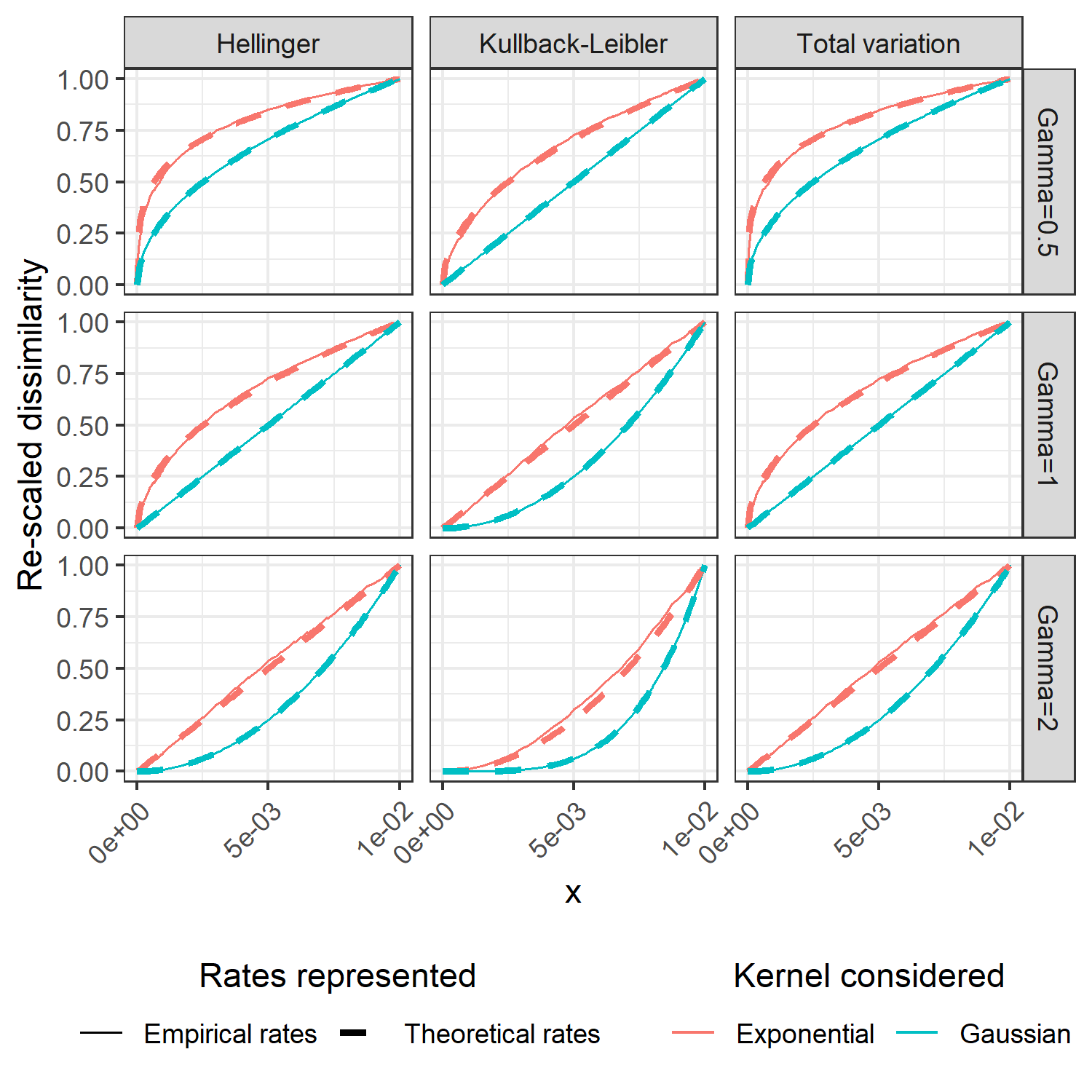
Figure 2: Visualising $\mathbb{E}\left[\mathfrak{D}\left(\Xi_{0},\Xi_{\mathbf{x}^{\prime}}\right)^{\gamma}\right]$ (plain lines) and the theoretical bound (dotted lines) for both kernels, all three dissimilarities and $\gamma\in\{0.5,1,2\}$.

This figure support our claim that the bounds obtained previously in the paper are tight. We now continue working on synthetic fields, and check that our SLGP models allow for learning the underlying fields.

4.2.2 Impact on learning the density field

We consider two density valued-fields, perfectly known, represented in Figure 3. We obtain them by applying the spatial logistic density transformation to realizations of GPs with the two previous kernels. The index spaces we consider here are $D=[0,1]$, $\mathcal{T}=[0,1]$.

We run the density field estimation, without hyper-parameters estimation. Figures displaying the mean posterior field are available in Figure 4 for the first reference field and in Appendix F, Figure 8 for the second. We observe that higher sample size seems to yield a better estimation as the models manages to capture the shape and modalities of the true density field.

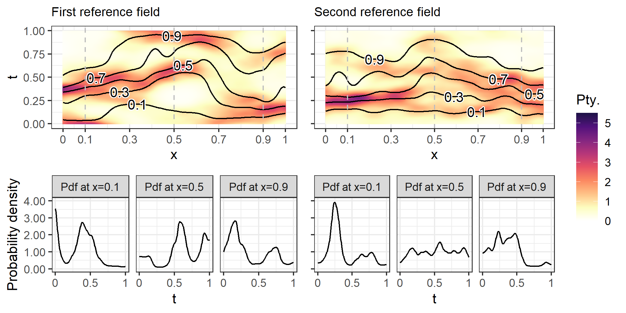
Figure 3: Representation of the two density fields used as reference: heat-map of the probability density field $f_{1}(\mathbf{x},t)$ and $f_{2}(\mathbf{x},t)$ with main quantiles of the field (top) and probability density functions over slices at $\mathbf{x}\in\{0.1,0.5,0.9\}$ (bottom).

Figure 4: Results for the first reference field. [Top figures:] Heat-map of the mean posterior probability density field with main quantiles and sample used. [Bottom figures:] 100 realizations of the posterior pdf (thin blue lines), posterior mean (blue dotted line) and true pdf (red) at $\mathbf{x}\in\{0.1,0.5,0.9\}$.

We expect the goodness of fit of our density estimation procedure to increase with the number of available observations. Since we only consider finite rank GP, the order $p$ (number of Fourier components used) may also determine how precise our estimation can be. In order to quantify the prediction error for different sample sizes and GP’s order, we define an Integrated Hellinger distance to measure dissimilarity between two probability density valued fields $f(\mathbf{x},\cdot)$ and $f^{\prime}(\mathbf{x},\cdot)$:

$$d_{IH}^{2}(f(\mathbf{x},\cdot),f^{\prime}(\mathbf{x},\cdot))=\frac{1}{2}\int_{D}\int_{\mathcal{T}}\left(\sqrt{f(\mathbf{v},u)}-\sqrt{f^{\prime}(\mathbf{v},u))}\right)^{2}\,du\,d\mathbf{v}$$ (46)

In Fig. 5, we display the distribution of $d_{IH}$ between true and estimated fields for various sample sizes and SLGP orders. We see that the errors are comparable for small sample sizes. The order becomes limiting when more observations are available, as those of the considered SLGPs relying on the smallest numbers of basis functions appear to struggle to capture small scale variations.

Although the goodness of fit are often comparable when few observations are available, when a numerous data are used, the order becomes limiting. We attribute this threshold phenomenon to the SLGP being unable to model small scale variations.

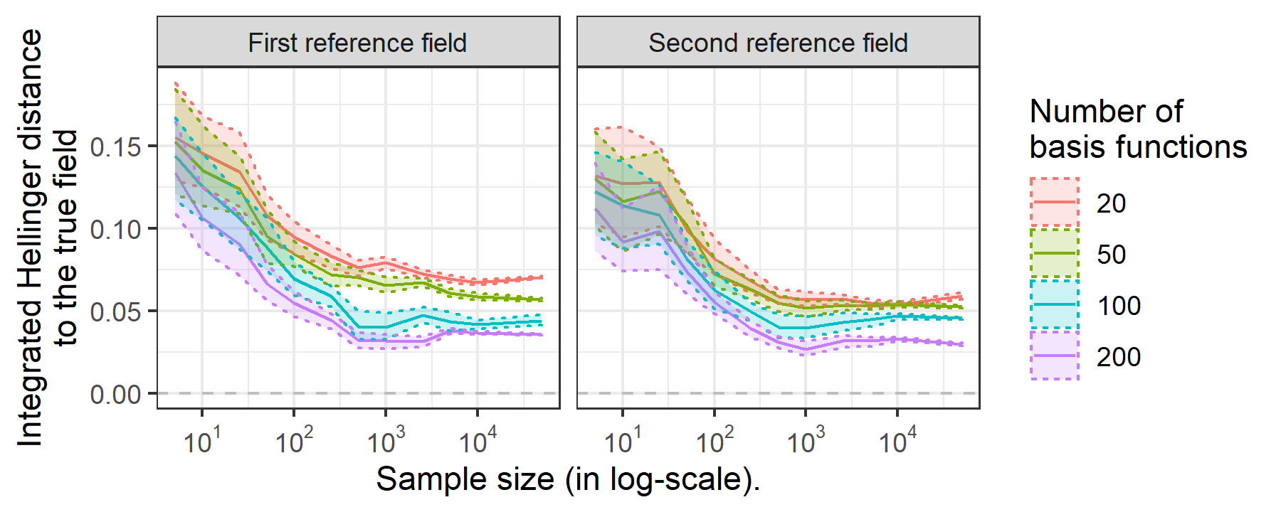
Figure 5: Integrated Hellinger distance distribution for different sample sizes and process orders.

4.3 Application to a meteorological dataset

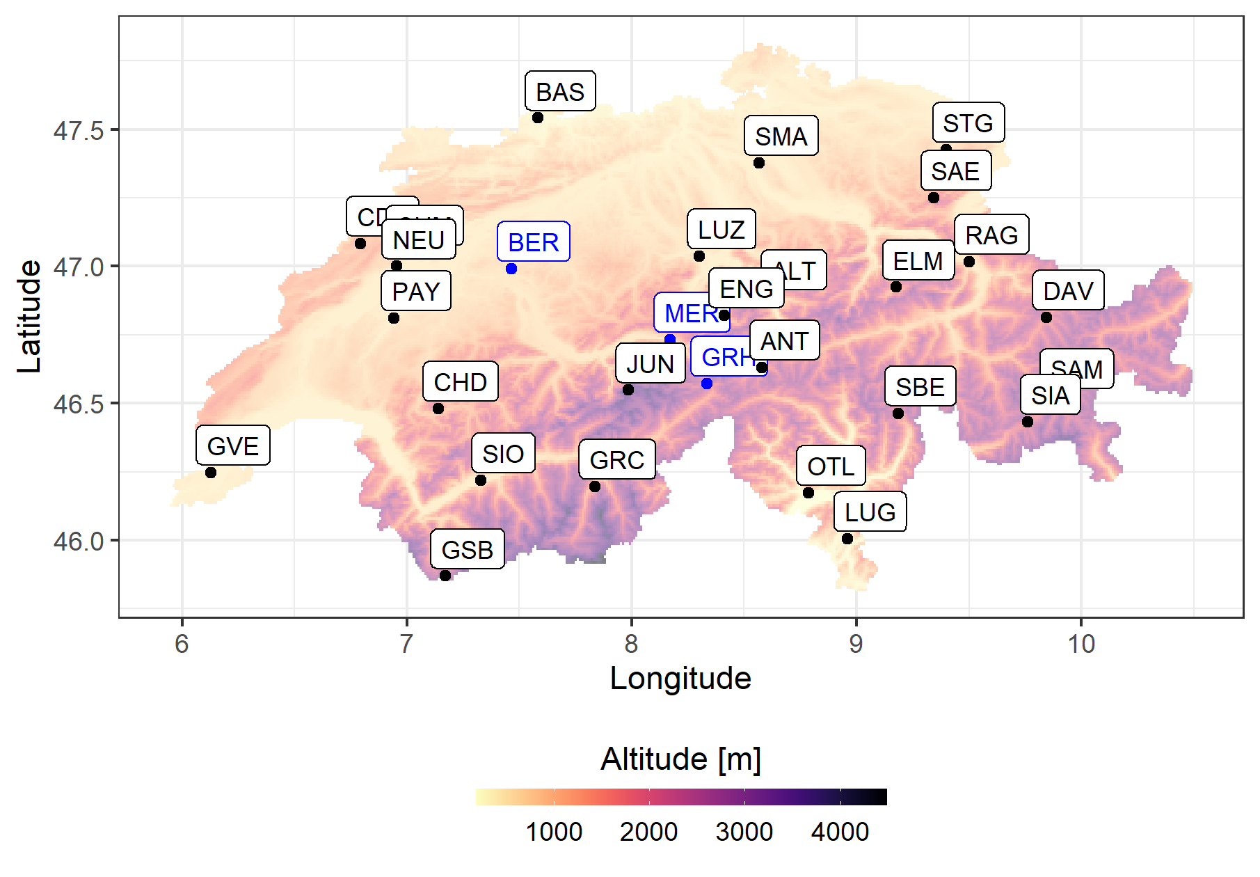
Figure 9: Map of Switzerland showing the 29 Stations present in the data-set, the stations not used to train the model are in blue.

We present an application on a data-set of temperatures in Switzerland. This application is by no mean a real forecasting application, and its only aim is to illustrate the applicability of the SLGP density estimation on real data. Our data consist in daily average temperatures in 2019, at 29 stations in Switzerland (represented in Appendix F, Figure 9). We consider that the distribution of these temperatures depends on the latitude, longitude and altitude of the station, and we fit the SLGP model on all the stations but three. Since we are not taking the date into account, we are actually working with marginal distributions.
An example of the available data is displayed in Appendix F, Figure 9

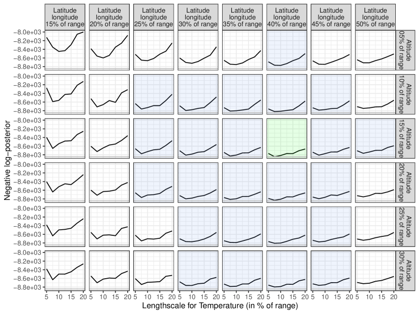
Figure 10: Showing the values of the negative log-likelihood when varying the lengthscale parameters for Latitude/Longitude, Altitude and Temperature. The panel achieving the minimum is highlighted in green, the panels whose smallest values are less than 1% away from the minimum are in light blue.

The temperature data-set is provided by MeteoSwiss [31] and the topographical data is provided by the Federal Office of Topography [32]. We used a 250 Fourier features (i.e. 500 basis functions) for a Matérn 5/2 kernel in this estimation, and considered only centred Gaussian Processes. We specify a finite-rank GP with 250 random Fourier features (i.e. 500 basis functions) drawn from the spectral density of a Matérn 5/2 kernel. We estimated the hyperparameters with a grid-search (by defining a grid of lengthscales values and running MAP estimation for each instance of the hyperparameters, then retaining the best candidate). The variance parameter, on the other hand, was selected to ensure numerical stability of the prior. One can refer to Appendix F, Figure 10 for the negative-log-posterior profiles. With this approach, we identify promising values of the lengthscale for latitude and longitude to be at $40\%$ of the range, while it is at $15\%$ for the altitude and $7.5\%$ for the temperature value.

In the main body of the paper, we display estimation results at stations to allow comparison with available data. However, SLGP modelling is a powerful tool that allows for predicting the density field over the whole domain (here, the whole of Switzerland). We dedicated Appendix F to illustrating further the full capabilities of our model.

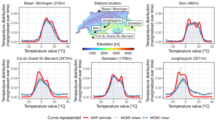
Figure 6: SLGP trained on 26 meteorological stations (365 observations each). We display for 5 stations in the training set: the histogram of the available data (blue), realizations drawn from the posterior (grey lines) and posterior mean (red line). For each station, we specify its elevation above sea level.

Let us start with the model displayed in Figure 6. For all the station, the MAP estimates follow the available histograms quite closely. However, it appears that the MCMC draws have more variability and sometimes struggle to reproduce all the modes. In particular, it still puts non negligible probability mass on every region of the domain. In addition to this artefact, it appears that at Col du grand St-Bernard, the model fails to reproduce the mode around 12 °C. This motivated us to pay particular attention to study stations of interest close to the Col du grand St-Bernard to see if we could partly explain this discrepancy between data and model predictions. Namely, we considered Sion (the closest station overall) and Jungfraujoch (closest station located at a mountain peak). This motivated us to pay particular attention to study stations of interest close to the Col du grand St-Bernard to see if we could partly explain this discrepancy between data and model predictions. Namely, we considered Sion (the closest station overall) and Jungfraujoch (closest station located at a mountain peak). It appeared that the distribution of temperatures in Jungfraujoch is clearly unimodal and that the SLGP model managed to capture this uni-modality. It suggests that the absence of the second mode at Col du Grand St-Bernard might be a simple consequence of the relative proximity of the two stations, both in latitude/longitude and in altitude.

Let us also note that the Jungfraujoch and the Col du Grand St-Bernard are respectively on the north slope, and the south side of their respective locations. Incorporating this information in the model might prove useful to yield better predictions, in particular at the considered stations.

We also make predictions at the three stations that we left out of the data set, to see whether the SLGP model manages to extrapolate at new locations. We observe, when comparing estimations performed at locations where data were available (Fig. 6) or not (Fig. 7) that the resulting random densities present more variability at stations left out of the training set, a desirable feature.

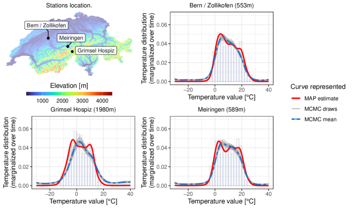
Figure 7: SLGP predictions for 3 stations out of the training set: histogram of the available data (blue), realizations drawn from the posterior (grey lines) and posterior mean (red line). For each station, we specify its elevation above sea level.

These results call for principled approaches for the evaluation of probabilistic predictions of probability density functions, a topic that seems in its infancy. While visual inspections suggest a fair extrapolation skill, there clearly remains room for improvement, opening the way for further work on modelling and implementation choices.

In particular, we noticed the presence of some artefacts in density field estimation. There seems to be two types of them. The first ones are artefacts close to the tails of the distribution. We see in Fig. 6 and 7 that the estimated pdf tend to increase close to the bounds of the domain $\mathcal{T}$. We suspect that this might be due to the fact that we used centred GPs whose behaviour are not constrained out $\mathcal{T}$. The other issue is mostly present in 7, for the stations Bern and Meiringen. We see two relatively, but not negligible small peaks close to -20°, a phenomenon that might come from the influence of other close stations on the prediction.

The specification of the topographical and other variables to be incorporated in the spatial index as well as the chosen families of covariance kernel hence appear to be of crucial importance regarding the resulting model and predictions. Also, the incorporation of trends appears as a meaningful avenue of research to be further explored to increase the realism of SLGP models.

5 Conclusion and discussions

In this paper, we investigated a class of models for non-parametric density field estimation. We revisited the Logistic Gaussian Process (LGP) model from the perspective of random measures, thoroughly investigating its relation to the underlying random processes and achieving some characterization in terms of increment covariances. We then built upon these investigations to further study Spatial LGP models, with a focus on their relationships with random measure fields. We demonstrated that when the underlying random field is continuous, SLGPs are characterised among random field of probability densities by the Gaussianity of associated log-increments.

Due to this particular structure, the SLGPs inherit their spatial regularity properties directly from the (Gaussian) field of increments of their log. This allowed us to leverage the literature of Gaussian Processes and Gaussian Measures to derive SLGP properties. We extended the notion of mean-square continuity to random measure fields and established sufficient conditions on covariance kernels underlying SLGPs for associated models to enjoy such properties.

We presented in Appendix E an implementation of the density field estimation that accommodates the need to estimate hyper-parameters of the model as well as the computational cost of this estimation. Our approach relies on Random Fourier Features, and we demonstrated its applicability of this approach in synthetic cases as well as on a meteorological application.

Several directions are foreseeable for future research. Extensive posterior consistency results as well as contraction rates are already available for LGPs [44, 47] and could be extended to the setting of SLGPs. We note that the posterior consistency is already studied when the index $\mathbf{x}$ is considered as random (as presented in Appendix D, following Pati et al. 2013 [34]), but the case of deterministic $\mathbf{x}$ is still to be studied, as well as the posterior contraction rates. An analysis of the misspecified setting could complete such analysis [24]. Our study of the spatial regularity properties of the SLGP could also be complemented, as noted in Remark 9.

In addition, further work towards evaluating the predictive performance of our model is needed. So far, we only relied on a squared integrated Hellinger distance for analytical settings where the reference field was known, and on qualitative and visual validation for the meteorological application. Comparing samples to predicted density fields calls for investigations in the field of scoring probabilistic forecasts of (fields of) densities. Therefore, evaluating the performances of the SLGP under several kernel settings, and comparing them to each other and to baseline methods is another main research direction.

As for implementation, we already highlighted in the Section 4, that the current implementation leaves room to improvement. So far, choosing the basis functions in the finite rank implementation, the hyper-parameters prior, the trend of the GP, and even the range $\mathcal{T}$ to consider was done mostly thanks to expert knowledge or trial and errors. We would greatly benefit from development in the methodology, as this might reduce the occurrence of artefacts thus improving the quality of predictions. A more efficient implementation would also allow us to use the SLGP model at higher scales (i.e. with more data points and higher dimensions).

The SLGP could be highly instrumental for Bayesian inference, even more so as the latter progress would be achieved. We already started exploring its applicability to stochastic optimisation [15], and are optimistic about the SLGP’s potential for speeding up Approximate Bayesian Computations [14]. Indeed, the flexibility of the non-parametric model allows for density estimation and it allows us to generate plausible densities. Having a generative model proves to be very beneficial, as it allows, for instance to derive experimental designs [4].

[Acknowledgments] This contribution is supported by the Swiss National Science Foundation project number 178858. Calculations in Section 4.2 were performed on UBELIX (http://www.id.unibe.ch/hpc), the HPC cluster at the University of Bern.
The authors would like to warmly thank Wolfgang Polonik for his time and his review of an earlier version of this paper. They are also grateful to Ilya Molchanov and Yves Deville for their knowledgeable and insightful comments.

Appendix A Some background properties and definitions.

A.1 About Gaussian Processes

A.1.1 Definitions on (Gaussian) random fields

We recall the definition of a Gaussian random field (a.k.a. Gaussian Process) in a general context.

Definition A.1 (Gaussian Process).

Let $S$ be a generic set. A collection of real-valued random variables $(Z_{s})_{s\in S}$ defined on a common probability space $(\Omega,\mathcal{F},P)$ is a Gaussian Process (GP) if its finite-dimensional distributions are Gaussian, meaning that for all $n\geq 1$ $s_{1},...,s_{n}\in S$, the random vector $(Z_{s_{1}},\dots,Z_{s_{n}})$ has a multivariate gaussian distribution.

The distribution of a Gaussian process is fully characterised by its mean function defined over $S$: $m(s)=\mathbb{E}[Z_{s}]$ and its covariance function (also called covariance kernel) $k$ defined by $k(s,s^{\prime}):=\text{Cov}(Z_{s},Z_{s^{\prime}})$ for any $s,s^{\prime}\in S$. In the document, we also used the following notions on Random Fields:

Definition A.2 (Separable Random Field as defined in [16]).

A random field $Z$ over the probability space $(\Omega,\mathcal{A},P)$ indexed by $S$ is called separable if there exists a countable dense subset $D\subset S$ and a set $N\subset\mathcal{A}$ of probability $0$ so that for any open set $E\subset S$ and any closed set $B\subset\mathbb{R}$, the two sets:

$$A_{B,I}=\left\{\omega:Z_{s}(\omega)\in B,\ \forall s\in E\right\}$$

$$A_{B,I\cap D}=\left\{\omega:Z_{s}(\omega)\in B,\ \forall s\in E\cap D\right\}$$

differ from each other only on a subset of N.

Definition A.3 (Versions of a random field).

Let $Z_{s}^{(1)}$ and $Z_{s}^{(2)}$ be two random fields on some index set $I$ over the same probability space $(\Omega,\mathcal{A},P)$. If:

$$P[Z_{s}^{(1)}=Z_{s}^{(2)}]=1,\ \forall s\in S$$

then $Z_{s}^{(2)}$ is called a version (or modification) of $Z_{s}^{(1)}$. It is also said that $Z_{s}^{(1)}$ and $Z_{s}^{(1)}$ are stochastically equivalent, or that they are equal in distribution.

Definition A.4 (Indistinguishable random fields).

Let $Z_{s}^{(1)}$ and $Z_{s}^{(2)}$ be two random fields on some index set $SI$ over the same probability space $(\Omega,\mathcal{A},P)$. If:

$$P[Z_{s}^{(1)}=Z_{s}^{(2)},\ \forall s\in S]=1$$

then $Z_{s}^{(1)}$ is said to be indistinguishable from $Z_{s}^{(2)}$.

A.1.2 Trajectories of a Gaussian Process: boundedness and continuity

The bounds of Property (3.1) lead us to the study of GPs. We will leverage Dudley’s integral theorem [9] which gives a sufficient condition for a GP $Z\sim\mathcal{GP}(0,k)$ over a domain $S$ to admit a version with almost all sample path uniformly continuous on $(S,d_{Z})$, where $d_{Z}$ is the canonical semi-metric associated to $Z$:

$$d_{Z}^{2}(s,s^{\prime})=Var[Z(s)-Z(s^{\prime})],\ \forall(s,s^{\prime})\in S^{2}.$$ (47)

For $\epsilon>0$, denote by $N(\epsilon,I,d_{Z})$ the entropy number, i.e. the minimal number of (open) $d_{Z}$-balls of radius $\epsilon$ required to cover $S$.

Theorem A.5 (Dudley’s integral).

For a GP $Z\sim\mathcal{GP}(0,k)$ over a domain $I$ and $\epsilon>0$:

$$\mathbb{E}\left[\|Z\|_{\infty}\right]\leq 24\displaystyle\int_{0}^{\infty}\sqrt{\log(N(\epsilon,S,d_{Z}))}\,d\epsilon.$$ (48)

Furthermore, if the entropy integral on the right-hand side converges, then $Z$ has a version with uniformly continuous paths on $S$ almost-surely.

Remark 10.

We note that, for any metric $d$ on $S$, if $Z$ admits a version with almost all sample paths uniformly continuous on $(S,d_{Z})$ and if $d_{Z}$ is continuous with respect to $d$ then $Z$ also admits a version with almost all sample paths uniformly continuous on $(S,d)$.

Based on the Dudley’s Theorem above, we obtain that if a covariance kernel $k$ satisfies Condition 2, then the associated centred GP admits a version that is almost surely continuous. Additionally if the index space is compact, it is also almost surely bounded. This constitutes a classical result in stochastic processes literature, but is essential as it ensures the objects we will work with are well-defined. It allows us in turn to derive a bound for the expected value of the sup-norm of our increment field, and to leverage it for our main contribution for Section 3.1: proving the almost surely continuity of the SLGP.

Proposition A.6.

If a kernel $k$ defined on $D\times\mathcal{T}$ satisfies Condition 2, then $Z\sim\mathcal{GP}(0,k)$ admits a version with almost surely uniformly continuous sample paths.

For this proof, and the following ones, we will need to bound the entropy number coming into play in Dudley’s theorem.

Lemma A.7.

For $d\geq 1$, and $T$ a convex, compact subset of $\mathbb{R}^{d}$, we recall that if $\epsilon\geq\text{diam}(T)$, then $N(\epsilon,T,\|\cdot\|_{\infty})=1$. Let Vol be the volume, and $B_{1}^{d}$ the $d$-dimensional unit ball, we have:

$$\left(\frac{1}{\epsilon}\right)^{d}\frac{\text{Vol}(T)}{\text{Vol}(B_{1}^{d})}\leq N(\epsilon,T,\|\cdot\|_{\infty})$$ (49)

Additionally, if $\epsilon<\text{diam}(T^{d})$:

$$N(\epsilon,T,\|\cdot\|_{\infty})\leq\left(\frac{4}{\epsilon}\right)^{d}\frac{\text{Vol}(T)}{\text{Vol}(B_{1}^{d})}$$ (50)

Proof of proposition A.6.

We consider the canonical pseudo metric associated to $k$, as defined in 3.2 . The space $D\times\mathcal{T}$ being compact, Condition 2 can be simplified as in Remark 10. Hence, there exists $\widetilde{C}>0$ with:

$$d_{k}^{2}(\mathbf{y},\mathbf{y}^{\prime})=k(\mathbf{y},\mathbf{y})+k(\mathbf{y}^{\prime},\mathbf{y}^{\prime})-2k(\mathbf{y},\mathbf{y}^{\prime})\leq\widetilde{C}\cdot\|\mathbf{y}-\mathbf{y}^{\prime}\|_{\infty}^{\min(\alpha_{1},\alpha_{2})}$$ (51)

for all $\mathbf{y},\mathbf{y}^{\prime}\in(D\times\mathcal{T})^{2}$. Dudley’s integral theorem gives:

$$\mathbb{E}\left[\|Z\|_{\infty}\right]\leq 24\int_{0}^{\infty}\sqrt{\log\left(N(\epsilon,D\times\mathcal{T},d_{k})\right)}\,d\epsilon$$ (52)

We note that for $\epsilon\geq\sup\limits_{\mathbf{y},\mathbf{y}^{\prime}\in D\times\mathcal{T}}d_{k}(\mathbf{y},\mathbf{y}^{\prime})$, then $N(\epsilon,D\times\mathcal{T},d_{k})=1$.
It follows from Equation 51 that $N(\epsilon,D\times\mathcal{T},d_{k})\leq N\left(\left(\epsilon/\widetilde{C}\right)^{2/\beta},D\times\mathcal{T},\|\cdot\|_{\infty}\right)$.

$$\mathbb{E}\left[\|Z\|_{\infty}\right]\leq 24\displaystyle\int_{0}^{\sup d_{k}(\mathbf{y},\mathbf{y}^{\prime})}\sqrt{\log N\left(\left(\epsilon/\widetilde{C}\right)^{2/\beta},D\times\mathcal{T},\|\cdot\|_{\infty}\right)}\,d\epsilon$$ (53)

Applying Lemma A.7 and using the fact that for all $a>0,x>0,\log(a/x)\leq a/x$, we have:

$$\mathbb{E}\left[\|Z\|_{\infty}\right] \leq 24\displaystyle\int_{0}^{\sup d_{k}(\mathbf{y},\mathbf{y}^{\prime})}\sqrt{\log\dfrac{K}{\epsilon}^{2(d_{\mathcal{T}}+d_{D})/\beta}}\,d\epsilon$$ (54)

$$\leq 24\displaystyle\int_{0}^{\sup d_{k}(\mathbf{y},\mathbf{y}^{\prime})}\sqrt{\dfrac{2(d_{\mathcal{T}}+d_{D})}{\beta}\log\dfrac{K}{\epsilon}}\,d\epsilon$$ (55)

$$\leq 24\sqrt{\dfrac{2(d_{\mathcal{T}}+d_{D})}{\beta}}\displaystyle\int_{0}^{\sup d_{k}(\mathbf{y},\mathbf{y}^{\prime})}\sqrt{\dfrac{K}{\epsilon}}\,d\epsilon<\infty$$ (56)

where $K:=\tilde{C}4^{\beta/2}\dfrac{\text{Vol}(D\times\mathcal{T})}{\text{Vol}(B_{1}^{d_{D}+d_{\mathcal{T}}})}>0$. The convergence of the integral induces that $Z$ admits a version with sample path almost surely bounded and uniformly continuous on $(D\times\mathcal{T},d_{k})$.

Then, as $d_{k}$ is continuous with respect to $\|\cdot\|_{\infty}$, it also induces that $Z$ admits a version with sample path almost surely bounded and uniformly continuous on $(D\times\mathcal{T},\|\cdot\|_{\infty})$. ∎

Remark 11.

We considered a centred GP in the previous proposition, as the influence of the mean is easy to rule out. Indeed, for $Z$ a centred GP and $m$ a function, the non-centred GP defined by $m+Z$ is continuous almost surely if $m$ is continuous and $W$ is continuous almost surely.

A.1.3 Gaussian measures on a Banach space

We also leverage some results about Gaussian measures on Banach spaces, namely Fernique theorem. The results listed in this subsection were adapted from [18].

Definition A.8 (Gaussian measure on a Banach space).

A probability measure $\mu$ over a Banach space $\mathfrak{B}$ is Gaussian if and only if for all $\ell\in\mathfrak{B}^{*}$ (the topological dual of $\mathfrak{B}$, i.e. the space of continuous linear forms on $\mathfrak{B}$), the push-forward measure $\mu\circ\ell^{-1}$ (of $\mu$ through $\ell$) is a Gaussian measure over $\mathbb{R}$.

One first result that is interesting for us is Fernique’s theorem.

Theorem A.9 (Fernique 1970).

Let $\mu$ be any probability measure on a separable Banach space $\mathfrak{B}$ and $R:\mathfrak{B}^{2}\rightarrow\mathfrak{B}^{2}$ be the rotation defined by:

$$\forall y,y^{\prime}\in\mathfrak{B}^{2},\ R(y,y^{\prime})=\left(\dfrac{y+y^{\prime}}{\sqrt{2}},\dfrac{y-y^{\prime}}{\sqrt{2}}\right).$$

If $\mu$ satisfies the invariance condition:

$$R^{*}(\mu\otimes\mu)=\mu\otimes\mu.$$

Then, there exists $\alpha>0$ such that $\int_{\mathfrak{B}}\exp(\alpha\|x\|^{2})\mu(\,dx)<\infty$.

The theorem is stated for any probability measure, in particular it holds for a Gaussian Measure, hence the following proposition also taken from [18].

Proposition A.10.

There exist universal constants $\alpha$, $K>0$ with the following properties. Let $\mu$ be a Gaussian measure on a separable Banach space $\mathfrak{B}$ and let $f:\mathbb{R}^{+}\rightarrow\mathbb{R}^{+}$ be any measurable function such that $f(x)\leq C_{f}\exp(\alpha x^{2})$ for every $x\geq 0$. Then, with $M=\int_{B}\|x\|\mu(\,dx)$ denoting the first moment of $\mu$, one has the bound $\int_{\mathfrak{B}}f(\|x\|/M)\mu(\,dx)\leq KC_{f}$

One of the corollary of this theorem is the following : a Gaussian measure admits moments (in a Bochner sense) of all orders.

In our setting, the following proposition will also prove handy to derive the almost sure continuity of our SLGP.

Proposition A.11.

Let $\mathfrak{B}$ be a separable Banach space, $S$ be a compact and convex subset of $\mathbb{R}^{d}$, and let $(Z_{s})_{s\in S}$ be a collection of $\mathfrak{B}$-valued Gaussian random variables such that

$$\mathbb{E}[\|Z_{s}-Z_{s^{\prime}}\|]\leq C\|s-s^{\prime}\|^{\alpha}$$ (57)

for some $C>0$ and some $\alpha\in(0,1]$. There exists a unique Gaussian measure $\mu$ on $\mathcal{C}(T,\mathfrak{B})$ such that any $(\tilde{Z}_{s})_{s\in S}$ having measure $\mu$ is a version of $Z$. Furthermore, $\tilde{Z}$ is almost surely $\beta$-Hölder continuous for every $\beta<\alpha$.

A final property of GPs that we will leverage in this work is the following.

Proposition A.12 (Small ball probabilities for a Gaussian process).

If $Z\sim\mathcal{GP}(0,k)$, is such that $\|Z\|_{\infty}<\infty$ a.s, then for all $\epsilon>0$:

$$P\left[\|Z\|_{\infty}<\varepsilon\right]>0$$ (58)

Moreover if $f$ is an element of the reproducing kernel Hilbert space of $k$, then for all $\epsilon>0$:

$$P\left[\|Z-f\|_{\infty}<\varepsilon\right]>0$$ (59)

The proof, as well as rates are available in [47]. This result allows one to relate properties of the process to its native space.

A.2 Basics of random measures.

Since our work explores the relationships between Random Measures (RM) and LGP (and later SLGP), we briefly recall some basic properties and definitions of (locally finite) random measures. We rely on the definitions from [23]. In the terminology of [23], our sample space of interest is here the space $\mathcal{T}$, equipped with the Euclidean metric (and hence Polish by the compactness assumption) and the corresponding Borel $\sigma$-algebra is $\mathcal{B}(\mathcal{T})$.

Definition A.13 (Considered sigma-field on probability measures on $(\mathcal{T},\mathcal{B}(\mathcal{T}))$).

We denote $\mathfrak{M}$ the collection of all probability measures on $(\mathcal{T},\mathcal{B}(\mathcal{T}))$, and take the $\sigma$-field $\mathcal{M}$ on $\mathfrak{M}$ to be the smallest $\sigma$-field that makes all maps $M\mapsto M(B)$ from $\mathfrak{M}$ to $\mathbb{R}$ measurable for $B\in\mathcal{B}(\mathcal{T})$.

Definition A.14 (Random Measures).

A random measure $\Xi$ is a random element from $(\Omega,\mathcal{F},P)$ to $(\mathfrak{M},\mathcal{M})$ such that for any $\omega\in\Omega\setminus N$, where $N$ is a $P$-null set, we have:

$$\Xi\left(\tilde{B};\omega\right)<\infty\text{ for all (bounded) measurable sets }\tilde{B}\in\mathcal{B}(\mathcal{T})$$ (60)

Note that here the term bounded is between parentheses as $\mathcal{T}$ is assumed compact and so all elements of $\mathcal{B}(\mathcal{T})$ are bounded. Among the motivations listed for the choice of this structure, we retain that the $\sigma$-field $\mathcal{M}$ is identical to the Borel $\sigma$-field for the weak topology of $\mathfrak{M}$. This structure ensures that the random elements $\Xi$ considered are regular conditional distributions on $(\mathcal{T},\mathcal{B}(\mathcal{T}))$:

1. For any $\omega\in\Omega$, the mapping $B\mapsto\Xi\left(B;\omega\right)$ is a measure on $(\mathcal{T},\mathcal{B}(\mathcal{T}))$.

2. For any $B\in\mathcal{B}(\mathcal{T})$, $\omega\mapsto\Xi\left(B;\omega\right)$ is $(\Omega,\mathcal{F})$-$(\mathbb{R},\mathcal{B}(\mathbb{R}))$ measurable.

Another strong advantage of this choice of measurability structure lies in the fact that if the state space $\mathcal{T}$ is equiped with a localizing structure, then the class of Probability Measures is a measurable subspace. The localizing structure arises naturally in our setting, as we can simply equip $\mathcal{T}$ with the class of all (bounded) Borel sets.

Finally, we also make a simple remark:

Remark 12 (RMs seen as scalar random fields).

We can see a RM $\Xi$ as a particular instance of a scalar-valued random field indexed by $\mathcal{B}(\mathcal{T})$, namely $\left(\Xi\left(B\right)\right)_{B\in\mathcal{B}(\mathcal{T})}$. Therefore it is natural to revisit the notions of equality in distribution and of indistinguishability for RMs. In particular, we will call two random measures $\Xi$ and $\tilde{\Xi}$ indistinguishable from one another if and only if:

$$P\left[\Xi\left(B\right)=\tilde{\Xi}(B),\ \forall B\in\mathcal{B}(\mathcal{T})\right]=1$$ (61)

Appendix B A deeper look at the Logistic Gaussian Process.

B.1 A short history of LGP models

The list intends to summarise the theoretical framework in which the previous contributions took place. It is ordered by publication date, we look at measurability and other assumptions underlying the respective LGP constructions, as well as the main contribution of the papers. In particular, we focus on whether the stochastic process the authors define has sample paths that are probability density functions, and if so, whether the papers consider some (response) measurable space suitable to accommodate such objects.

• In the seminal paper [27], the authors the LGP was studied in a uni-dimensional setting, with $\mathcal{T}$ being a compact interval. The authors considered the a.s. surely continuous GPs with exponential covariance kernel.

• Later, the authors of [25] claimed that LGPs should be seen as positive-valued random functions integrating to 1 but fail to provide an explicit construction of the corresponding measure space. They extended their construction to derive a generalized logistic Gaussian processes (gLGP) and elegant formulations of the posterior distribution of the gLGP conditioned on observations were derived. Numerical approaches for calculating the Bayes estimate were proposed, constituting the starting point of the follow-up paper [26].

• In [44], the LGP was introduced from a hierarchical Bayesian modelling perspective, allowing in turn to handle the estimation of GP hyper-parameters. This paper considered a separable GP $Z$ that is exponentially integrable almost surely, stating that the LGP thus takes values in $\mathcal{A}(\mathcal{T})$. The main result in the paper is that the considered hierarchical model achieves weak and strong consistency for density estimation at functions that are piece-wise continuous. It is completed by another paper, [43], where the authors propose a tractable implementation of the density estimation with such a model. Let us note that the GP’s separability alleviates some technicalities regarding the measurability assumptions to consider, and having $\int_{\mathcal{T}}e^{Z_{u}}\,d\lambda(u)<\infty$ a.s. allows us to state that LGP realisations are PDFs almost surely.

• Meanwhile, the authors of [47] work with a bounded-functions-valued GPs, which allowed it to be viewed as a Borel measurable map in the space of bounded functions of $\mathcal{T}$ equipped with the sup-norm. This paper derived concentration rates for the posterior of the LGP. With these assumptions, the LGP can be considered as a Borel measurable map in the same space as $Z$ and is guaranteed to have sample paths that are bounded probability density functions.

This short review emphasizes the lack of consensus regarding the LGP’s definition including underlying structures and assumptions. It is interesting to note that in [47], the authors require $Z$ to be bounded surely, whereas the authors of the three other papers worked with almost sure properties of $Z$ (mostly, the almost surely continuity of the process).

Appendix C Details of the proofs in Section 3

Proof of Proposition 3.4.

For fixed $(\mathbf{x},\mathbf{x}^{\prime})\in D^{2}$ and $Z\sim\mathcal{GP}(0,k)$, we note $d_{\mathbf{x},\mathbf{x}^{\prime}}$ the canonical semi-metric associated to $Z_{\mathbf{x},\cdot}-Z_{\mathbf{x}^{\prime},\cdot}$, defined by:

$$d_{\mathbf{x},\mathbf{x}^{\prime}}^{2}(t,t^{\prime})=\mathbb{E}\left[\left([Z_{\mathbf{x},t}-Z_{\mathbf{x}^{\prime},t}]-[Z_{\mathbf{x},t^{\prime}}-Z_{\mathbf{x}^{\prime},t^{\prime}}]\right)^{2}\right]\forall(t,t^{\prime})\in\mathcal{T}^{2}$$ (62)

Using the Hölder condition on $k$ we note that we have simultaneously:

$$d_{\mathbf{x},\mathbf{x}^{\prime}}^{2}(t,t^{\prime})\leq 3C\|\mathbf{x}-\mathbf{x}^{\prime}\|^{\alpha_{1}}_{\infty}\forall(t,t^{\prime})\in\mathcal{T}^{2}$$ (63)

$$d_{\mathbf{x},\mathbf{x}^{\prime}}^{2}(t,t^{\prime})\leq 4C\|t-t^{\prime}\|^{\alpha_{2}}_{\infty}\forall(t,t^{\prime})\in\mathcal{T}^{2}$$ (64)

By Dudley’s theorem, we can write :

$$\begin{array}[]{ll}M(\mathbf{x},\mathbf{x}^{\prime})&\leq 24\displaystyle\int_{0}^{\infty}\sqrt{\log(N(\epsilon,\mathcal{T},d_{\mathbf{x},\mathbf{x}^{\prime}}))}\,d\epsilon\\ &\leq 24\displaystyle\int_{0}^{D_{\mathbf{x},\mathbf{x}^{\prime}}(\mathcal{T})}\sqrt{\log(N(\epsilon,\mathcal{T},d_{\mathbf{x},\mathbf{x}^{\prime}}))}\,d\epsilon\\ \end{array}$$ (65)

where $D_{\mathbf{x},\mathbf{x}^{\prime}}(\mathcal{T})$ stands for the diameter of $\mathcal{T}$ with respect to the canonical semi-metric associated to $d_{\mathbf{x},\mathbf{x}^{\prime}}$. As $\ d_{\mathbf{x},\mathbf{x}^{\prime}}^{2}(t,t^{\prime})\leq 4C\|t-t^{\prime}\|_{\infty}^{\alpha_{2}}$, we can combine the bounds stated in Lemma (A.7) with the inequality

$$N(\epsilon,\mathcal{T},d_{\mathbf{x},\mathbf{x}^{\prime}})\leq N\left(\left(\dfrac{\epsilon}{4C}\right)^{2/\alpha_{2}},\mathcal{T},\|\cdot\|_{\infty}\right)$$

It follows that

$$M(\mathbf{x},\mathbf{x}^{\prime})\leq 24\sqrt{\dfrac{2d_{\mathcal{T}}}{\alpha_{2}}}\displaystyle\int_{0}^{D_{\mathbf{x},\mathbf{x}^{\prime}}(\mathcal{T})}\sqrt{\log\left(\dfrac{K}{\epsilon}\right)}\,d\epsilon$$ (66)

where $K:=C4^{1+\alpha_{2}/2}\left(\dfrac{\text{Vol}(\mathcal{T})}{\text{Vol}(B_{1}^{d_{\mathcal{T}}})}\right)^{\alpha_{2}/(2d_{\mathcal{T}})}$ and $B_{1}^{d_{\mathcal{T}}}$ stands for the $d_{\mathcal{T}}$-dimensional unit ball for $\|\cdot|_{\infty}$. To further compute the right-hand term, we introduce the error function, defined as $\text{erf}(x)=\dfrac{2}{\sqrt{\pi}}\int_{0}^{x}e^{-t^{2}}\,dt$.

$$\displaystyle\int_{0}^{D_{\mathbf{x},\mathbf{x}^{\prime}}(\mathcal{T})}\sqrt{\log\left(\dfrac{K}{\epsilon}\right)}\,d\epsilon=\left[\epsilon\sqrt{\log\dfrac{K}{\epsilon}}-\dfrac{\sqrt{\pi}}{2}K\text{erf}\left(\sqrt{\log\dfrac{K}{\epsilon}}\right)\right]^{D_{\mathbf{x},\mathbf{x}^{\prime}}(\mathcal{T})}_{0}$$ (67)

$$=D_{\mathbf{x},\mathbf{x}^{\prime}}(\mathcal{T})\sqrt{\log\dfrac{K}{D_{\mathbf{x},\mathbf{x}^{\prime}}(\mathcal{T})}}+K\displaystyle\int_{\sqrt{\log(K/D_{\mathbf{x},\mathbf{x}^{\prime}}(\mathcal{T}))}}^{\infty}e^{-t^{2}}\,dt$$ (68)

Since for $y>0$, $\frac{2}{\sqrt{\pi}}\int_{y}^{\infty}e^{-t^{2}}\,dt\leq e^{-y^{2}}$, we also have:

$$M(\mathbf{x},\mathbf{x}^{\prime})\leq 24\sqrt{\dfrac{2d_{\mathcal{T}}}{\alpha_{2}}}\left(D_{\mathbf{x},\mathbf{x}^{\prime}}(\mathcal{T})\sqrt{\log\dfrac{K}{D_{\mathbf{x},\mathbf{x}^{\prime}}(\mathcal{T})}}+\dfrac{\sqrt{\pi}D_{\mathbf{x},\mathbf{x}^{\prime}}(\mathcal{T})}{2K}\right)$$ (69)

Then, for any $0<\delta<\dfrac{\alpha_{1}}{2}$, $D$ being compact and considering that

$$y\left(\log(K/y)\right)^{1/2}\underset{y\to 0}{=}o\left(y^{1-2\delta/\alpha_{1}}\right)$$

we can conclude that there exists $K_{\delta}$ such that:

$$\begin{array}[]{rl}M(\mathbf{x},\mathbf{x}^{\prime})\leq&K_{\delta}\dfrac{1}{(3C)^{1/2-\delta/\alpha_{1}}}\left(D_{\mathbf{x},\mathbf{x}^{\prime}}(\mathcal{T})^{1-2\delta/\alpha_{1}}\right)\end{array}$$ (70)

Finally, by Equation 32, we have $D_{\mathbf{x},\mathbf{x}^{\prime}}(\mathcal{T})\leq\sqrt{3C}\|\mathbf{x}-\mathbf{x}^{\prime}\|^{\alpha_{1}/2}$, and we can conclude that:

$$\begin{array}[]{ll}M(\mathbf{x},\mathbf{x}^{\prime})\leq K_{\delta}\|\mathbf{x}-\mathbf{x}^{\prime}\|^{\alpha_{1}/2-\delta}\end{array}$$ (71)

∎

Proof of Theorem 3.7.

Let us consider $(\mathbf{x},\mathbf{x}^{\prime})\in D^{2}$ and $\gamma>0$. By Lemma 3.1, there exists two constants $C_{KL},C_{TV}>0$ such that:

$$\begin{array}[]{c}\mathbb{E}\left[d_{H}((Y_{\mathbf{x},\cdot})_{,}Y_{\mathbf{x}^{\prime},\cdot})^{\gamma}\right]\leq\mathbb{E}\left[\|Z_{\mathbf{x},\cdot}-Z_{\mathbf{x}^{\prime},\cdot}\|_{\infty}^{\gamma}e^{\|Z_{\mathbf{x},\cdot}-Z_{\mathbf{x}^{\prime},\cdot}\|_{\infty}\gamma/2}\right]\\ \mathbb{E}\left[KL(Y_{\mathbf{x},\cdot},Y_{\mathbf{x}^{\prime},\cdot})^{\gamma}\right]\leq C_{KL}\mathbb{E}[f_{1}(\|Z_{\mathbf{x},\cdot}-Z_{\mathbf{x}^{\prime},\cdot}\|_{\infty})]\\ \mathbb{E}\left[d_{TV}(Y_{\mathbf{x},\cdot},Y_{\mathbf{x}^{\prime},\cdot})^{\gamma}\right]\leq C_{TV}\mathbb{E}[f_{2}(\|Z_{\mathbf{x},\cdot}-Z_{\mathbf{x}^{\prime},\cdot}\|_{\infty})]\end{array}$$ (72)

where $f_{1}(x)=x^{2\gamma}\left(1+x\right)^{\gamma}e^{\gamma x}$ and $f_{2}(x)=x^{2\gamma}\left(1+x\right)^{2\gamma}e^{\gamma x}$.

We consider the three functions, defined for $\gamma,M,y>0$:

$$\begin{array}[]{rl}f_{H,\gamma,M}(y)&=(My)^{\gamma}e^{\frac{M\gamma}{2}y}\\ f_{KL,\gamma,M}(y)&=(My)^{2\gamma}(1+My)^{\gamma}e^{M\gamma y}\\ f_{TV,\gamma,M}(y)&=(My)^{2\gamma}(1+My)^{2\gamma}e^{M\gamma y}\\ \end{array}$$ (73)

Then, if we consider $M(\mathbf{x},\mathbf{x}^{\prime})=\mathbb{E}\left[\|Z_{\mathbf{x},\cdot}-Z_{\mathbf{x}^{\prime},\cdot}\|_{\infty}\right]$, the previous inequalities can be rewritten as:

$$\begin{array}[]{c}\mathbb{E}\left[d_{H}(Y_{\mathbf{x},\cdot},Y_{\mathbf{x}^{\prime},\cdot})^{\gamma}\right]\leq\mathbb{E}\left[f_{H,\gamma,M(\mathbf{x},\mathbf{x}^{\prime})}\left(\dfrac{\|Z_{\mathbf{x},\cdot}-Z_{\mathbf{x}^{\prime},\cdot}\|_{\infty}}{M(\mathbf{x},\mathbf{x}^{\prime})}\right)\right]\\ \mathbb{E}\left[KL(Y_{\mathbf{x},\cdot},Y_{\mathbf{x}^{\prime},\cdot})^{\gamma}\right]\leq C_{KL}\cdot\mathbb{E}\left[f_{KL,\gamma,M(\mathbf{x},\mathbf{x}^{\prime})}\left(\dfrac{\|Z_{\mathbf{x},\cdot}-Z_{\mathbf{x}^{\prime},\cdot}\|_{\infty}}{M(\mathbf{x},\mathbf{x}^{\prime})}\right)\right]\\ \mathbb{E}\left[d_{TV}(Y_{\mathbf{x},\cdot},Y_{\mathbf{x}^{\prime},\cdot})^{\gamma}\right]\leq C_{TV}\cdot\mathbb{E}\left[f_{TV,\gamma,M(\mathbf{x},\mathbf{x}^{\prime})}\left(\dfrac{\|Z_{\mathbf{x},\cdot}-Z_{\mathbf{x}^{\prime},\cdot}\|_{\infty}}{M(\mathbf{x},\mathbf{x}^{\prime})}\right)\right]\end{array}$$ (74)

By Fernique theorem (cf proposition A.10), there exists universal constant $\alpha$, $K>0$, as well as $C_{H,\gamma,M},C_{KL,\gamma,M}$ and $C_{TV,\gamma,M}>0$ such that:

$$\begin{array}[]{c}\mathbb{E}\left[d_{H}(Y_{\mathbf{x},\cdot},Y_{\mathbf{x}^{\prime},\cdot})^{\gamma}\right]\leq C_{H,\gamma,M(\mathbf{x},\mathbf{x}^{\prime})}\cdot K\\ \mathbb{E}\left[KL(Y_{\mathbf{x},\cdot},Y_{\mathbf{x}^{\prime},\cdot})^{\gamma}\right]\leq C_{KL}\cdot C_{KL,\gamma,M(\mathbf{x},\mathbf{x}^{\prime})}\cdot K\\ \mathbb{E}\left[d_{TV}((Y_{\mathbf{x},\cdot})_{,}(Y_{\mathbf{x}^{\prime},\cdot})_{)}^{\gamma}\right]\leq C_{TV}\cdot C_{TV,\gamma,M(\mathbf{x},\mathbf{x}^{\prime})}\cdot K\end{array}$$ (75)

Detailed expressions of $C_{H,\gamma,M},C_{KL,\gamma,M}$ and $C_{TV,\gamma,M}$ are given below this proof, and were derived with the tightness of our bounds in mind. We note that these coefficients seen as functions of $M$ are continuous, strictly positive for any $M>0$ and that:

$$\begin{array}[]{c}C_{H,\gamma,M}\underset{M\to 0}{\sim}M^{\gamma}\left(\dfrac{\gamma}{2\alpha}\right)^{\gamma/2}\exp\left\{-\dfrac{\gamma}{2}\right\}\\ C_{KL,\gamma,M}\underset{M\to 0}{\sim}M^{2\gamma}\left(\dfrac{\gamma}{\alpha}\right)^{\gamma}\exp\left\{-\gamma\right\}\\ C_{TV,\gamma,M}\underset{M\to 0}{\sim}M^{2\gamma}\left(\dfrac{\gamma}{\alpha}\right)^{\gamma}\exp\left\{-\gamma\right\}\\ \end{array}$$ (76)

This equivalence allows us to state that for a given $\gamma>0$, there exists a rank $M_{0}>0$ and a constant $\kappa_{\gamma,1}>1$ such that for any $M<M_{0}$:

$$\begin{array}[]{ccc}C_{H,\gamma,M}\leq\kappa_{\gamma,1}M^{\gamma},&C_{KL,\gamma,M}\leq\kappa_{\gamma,1}M^{2\gamma},&C_{TV,\gamma,M}\leq\kappa_{\gamma,1}M^{2\gamma}\end{array}$$ (77)

We also observe that if $M$ is bounded, as $C_{H,\gamma,M},C_{KL,\gamma,M}$ and $C_{TV,\gamma,M}$ seen as function of $M$ are continuous and strictly positive, there exists a constant $\kappa_{\gamma,2}>0$ such that for values of $M\geq M_{0}$:

$$\begin{array}[]{ccc}C_{H,\gamma,M}\leq\kappa_{\gamma,2}M^{\gamma},&C_{KL,\gamma,M}\leq\kappa_{\gamma,2}M^{2\gamma},&C_{TV,\gamma,M}\leq\kappa_{\gamma,2}M^{2\gamma}\end{array}$$ (78)

Combining these two observations, and $M(\mathbf{x},\mathbf{x}^{\prime})$ being bounded, we conclude that for any $\gamma>0$ there exist $\kappa_{\gamma}$ such that:

$$\begin{array}[]{c}\mathbb{E}\left[d_{H}(Y_{\mathbf{x},\cdot},Y_{\mathbf{x}^{\prime},\cdot})^{\gamma}\right]\leq\kappa_{\gamma}M(\mathbf{x},\mathbf{x}^{\prime})^{\gamma}\\ \mathbb{E}\left[KL(Y_{\mathbf{x},\cdot},Y_{\mathbf{x}^{\prime},\cdot})^{\gamma}\right]\leq\kappa_{\gamma}M(\mathbf{x},\mathbf{x}^{\prime})^{2\gamma}\\ \mathbb{E}\left[d_{TV}(Y_{\mathbf{x},\cdot},Y_{\mathbf{x}^{\prime},\cdot})^{\gamma}\right]\leq\kappa_{\gamma}M(\mathbf{x},\mathbf{x}^{\prime})^{2\gamma}\\ \end{array}$$ (79)

This argument relies on an equivalence at zero. Therefore, it ensures that the convergence rates are not degraded when bounding $C_{H,\gamma,M},C_{KL,\gamma,M}$ and $C_{TV,\gamma,M}$, and that our bounds are still tight.

Finally, using proposition 3.4, stating that for all $\delta>0$, there exists $K_{\delta}$ such that:

$$\ M(\mathbf{x},\mathbf{x}^{\prime})\leq K_{\delta}\|\mathbf{x}-\mathbf{x}^{\prime}\|^{\alpha_{1}/2-\delta}_{\infty}$$ (80)

We conclude that for all $\gamma>0,\delta>0$, there exists a constant $K_{\gamma,\delta}$ such that:

$$\begin{array}[]{c}\mathbb{E}\left[d_{H}(Y_{\mathbf{x},\cdot},Y_{\mathbf{x}^{\prime},\cdot})^{\gamma}\right]\leq K_{\gamma,\delta}\|\mathbf{x}-\mathbf{x}^{\prime}\|^{\gamma\alpha_{1}/2-\delta}_{\infty}\\ \mathbb{E}\left[KL(Y_{\mathbf{x},\cdot},Y_{\mathbf{x}^{\prime},\cdot})^{\gamma}\right]\leq K_{\gamma,\delta}\|\mathbf{x}-\mathbf{x}^{\prime}\|^{\gamma\alpha_{1}-\delta}_{\infty}\\ \mathbb{E}\left[d_{TV}(Y_{\mathbf{x},\cdot},Y_{\mathbf{x}^{\prime},\cdot})^{\gamma}\right]\leq K_{\gamma,\delta}\|\mathbf{x}-\mathbf{x}^{\prime}\|^{\gamma\alpha_{1}-\delta}_{\infty}\\ \end{array}$$ (81)

∎

Finding the constants in Proof of Theorem 3.7.

For fixed $M$, $\gamma>0$, we consider the following three functions, for $x\geq 0$:

$$\begin{array}[]{rl}f_{H,\gamma,M}(x)&=(Mx)^{\gamma}e^{\frac{M\gamma}{2}x}\\ f_{KL,\gamma,M}(x)&=(Mx)^{2\gamma}(1+Mx)^{\gamma}e^{M\gamma x}\\ f_{TV,\gamma,M}(x)&=(Mx)^{2\gamma}(1+Mx)^{2\gamma}e^{M\gamma x}\\ \end{array}$$ (82)

For $\alpha>0$, we look for constants $C_{H,\gamma,M},C_{KL,\gamma,M},C_{TV,\gamma,M}$, satisfying:

$$\begin{array}[]{rl}f_{H,\gamma,M}(x)&\leq C_{H,\gamma,M}e^{\alpha x^{2}}\\ f_{KL,\gamma,M}(x)&\leq C_{KL,\gamma,M}e^{\alpha x^{2}}\\ f_{TV,\gamma,M}(x)&\leq C_{TV,\gamma,M}e^{\alpha x^{2}}\\ \end{array}$$ (83)

such constants satisfy:

$$\begin{array}[]{l}\sup\limits_{x\geq 0}\ g_{H,\gamma,M}(x):=f_{H,\gamma,M}(x)e^{-\alpha x^{2}}\leq C_{H,\gamma,M}\\ \sup\limits_{x\geq 0}\ g_{KL,\gamma,M}(x):=f_{KL,\gamma,M}(x)e^{-\alpha x^{2}}\leq C_{KL,\gamma,M}\\ \sup\limits_{x\geq 0}\ g_{TV,\gamma,M}(x):=f_{TV,\gamma,M}(x)e^{-\alpha x^{2}}\leq C_{TV,\gamma,M}\\ \end{array}$$ (84)

Studying the variations of $g_{H,\gamma,M}(x)$ simply involves finding the roots of a degree 2 polynomial and yields that this function attains its supremum at:

$$x_{H,\gamma,M}=\dfrac{M\gamma+2\sqrt{M^{2}\gamma^{2}+8\alpha\gamma}}{8\alpha}$$ (85)

Therefore a valid upper bound for :

$$C_{H,\gamma,M}=\left(Mx_{H,\gamma,M}\right)^{\gamma}\exp\left\{M\gamma\frac{x_{H,\gamma,M}}{2}-\alpha x_{H,\gamma,M}^{2}\right\}$$ (86)

This constant is optimal in the sense that it is the smallest constant satisfying inequality 84.

However, studying the variations of $g_{KL,\gamma,M}(x)$ and $g_{TV,\gamma,M}(x)$ is longer as it involves finding the roots of third degree polynomials. In order to simplify the constant, we use the simple property $1+x\leq e^{x}$ and introduce the bounds :

$$\begin{array}[]{l}g_{KL,\gamma,M}(x)\leq(Mx)^{2\gamma}e^{2M\gamma x-\alpha x^{2}}=:h_{KL,\gamma,M}(x)\\ g_{TV,\gamma,M}(x)\leq(Mx)^{2\gamma}e^{3M\gamma x-\alpha x^{2}}=:h_{TV,\gamma,M}(x)\\ \end{array}$$ (87)

These inequalities are tight at $Mx=0$.

Studying the variations of $h_{KL,\gamma,M}(x)$ and $h_{TV,\gamma,M}(x)$ simply involves finding the roots of a degree 2 polynomial and yields that this function attains their supremum at:

$$\begin{array}[]{l}x_{KL,\gamma,M}=\dfrac{M\gamma+\sqrt{M^{2}\gamma^{2}+4\alpha\gamma}}{2\alpha}\\ x_{TV,\gamma,M}=\dfrac{3M\gamma+\sqrt{9M^{2}\gamma^{2}+16\alpha\gamma}}{4\alpha}\end{array}$$ (88)

Therefore, we can take the bounds:

$$C_{KL,\gamma,M}=\left(Mx_{KL,\gamma,M}\right)^{2\gamma}\exp\left\{2M\gamma x_{KL,\gamma,M}-\alpha x_{KL,\gamma,M}^{2}\right\}$$ (89)

$$C_{TV,\gamma,M}=\left(Mx_{TV,\gamma,M}\right)^{2\gamma}\exp\left\{x_{TV,\gamma,M}-\alpha x_{TV,\gamma,M}^{2}\right\}$$ (90)

These bounds are tight around zero. ∎

Appendix D A result on posterior consistency

D.1 Basics of posterior consistency in the Bayesian literature

This Section aims at introducing the basic ideas and tools necessary to establish posterior consistency of a prior distribution. Posterior consistency is a desirable property as it ensures that provided enough data, a well-specified Bayesian model will recover the true data generating process.

We consider a parameter space $\Theta$, which does not need to be euclidean. Assuming that we have available observations, noted $\mathbf{Y}^{(n)}=\{\mathbf{Y}_{i}\}_{i=1}^{n}$. The probability distribution of $\mathbf{Y}^{(n)}$ is assumed to be controlled by a parameter $\theta$ and is noted $P_{\theta}^{(n)}$. Let $\Pi$ be a prior over $\Theta$.

Definition D.1 (Weak posterior consistency).

It is said that the prior $\Pi$ achieves weak posterior consistency at $\theta_{0}\in\Theta$ with respect to a given topology if for any weak neighbourhood $U$ of $\theta_{0}$:

$$\Pi\left[U|\mathbf{Y}^{(n)}\right]\xrightarrow[n\to\infty]{}1$$ (91)

almost surely under $P_{\theta_{0}}^{(n)}$

Remark 13.

It is common, but not necessary, to consider the observations $\mathbf{Y}^{(n)}$ to be independent, as it simplifies the expression of the distribution $P_{\theta_{0}}^{(n)}$.

This definition is quite general, and it is often difficult to prove consistency in a general setting. One really indispensable result for non-parametric and semi-parametric problems is Schwartz’s theorem. It leverages the Kullback-Leibler divergence. Schwartz’s method consists in a general method for establishing consistency and writes as follows:

Theorem D.2 (Schwartz, 1965).

Let $\{f_{\theta}:\theta\in\Theta\}$ be a class of densities and let $\mathbf{Y}_{1},\mathbf{Y}_{2},...$ be i.i.d. with density $f_{\theta_{0}}$, where $\theta_{0}\in\Theta$. Suppose for every neighbourhood $U$ of $\theta_{0}$, there is a test for $\theta=\theta_{0}$ against $\theta\not\in U$ with power strictly greater than the size. Let $\Pi$ be a prior on $\Theta$ such that for every $\epsilon>0$:

$$\Pi\left[\theta:KL(f_{\theta_{0}},f_{\theta})<\epsilon\right]>0$$ (92)

Then the posterior is consistent at $\theta_{0}$

Remark 14.

Schwartz’s theorem gives a sufficient condition for weak posterior consistency, however it is not a necessary condition.

Remark 15.

If $\Theta$ is itself a class of densities with $f_{\theta}=\theta$, then the condition on existence of tests in Schwartz’s theorem is satisfied if $\Theta$ is endowed with the topology of weak convergence.
More generally, existence of a uniformly consistent estimator implies the existence of such a test.

Finally, note that consistency is defined with respect to a given topology. Here, we define some topologies that will be relevant in this thesis.

Definition D.3 (Weak neighbourhood of a conditional density).

We define the weak convergence neighbourhood of a density field $p_{0}$ of pdfs on $\mathcal{T}$ indexed by $D$ through a sub-base. It is given for any bounded continuous function $g:D\times\mathcal{T}\to\mathbb{R}$ and any $\epsilon>0$ by:

$$V_{\epsilon,g}=\left\{f\in\mathcal{F}_{d}(D;\mathcal{T}),\left|\int_{D\times\mathcal{T}}gf-\int_{D\times\mathcal{T}}gf_{0}\right|<\epsilon\right\}$$ (93)

A weak neighbourhood base is formed by finite intersections of neighbourhoods of the above type.

Definition D.4 (Weak neighbourhood of a joint density).

We define the weak convergence neighbourhood of a joint density $h_{0}$ on $D\times\mathcal{T}$ through a sub-base. It is given for any bounded continuous function $g:D\times\mathcal{T}\to\mathbb{R}$ and any $\epsilon>0$ by:

$$W_{\epsilon,g}=\left\{h\in\mathcal{F}(D\times\mathcal{T}),\left|\int_{D\times\mathcal{T}}gh-\int_{D\times\mathcal{T}}gh_{0}\right|<\epsilon\right\}$$ (94)

A weak neighbourhood base is formed by finite intersections of neighbourhoods of the above type.

D.2 Posterior consistency for (logistic Gaussian) random measure fields

From now-on, we will consider that we have observations obtained by independent sampling of a reference field $p_{0}$ of pdfs on $\mathcal{T}$ indexed by $D$. By that, we mean that our dataset consist in $n$ couples of locations and observations $\{(\mathbf{x}_{i},t_{i})\}_{1\leq i\leq n}$, where the $\mathbf{x}_{i}$ are in $D$. Moreover, we assume the $t_{i}$’s are obtained by independent sampling of random variables $T_{i}$ with density $p_{0}(\mathbf{x}_{i},\cdot)$. The (random) vectors of observations are denoted by $\mathbf{T}=(T_{i})_{1\leq i\leq n}$ and $\mathbf{t}=(t_{i})_{1\leq i\leq n}$ respectively, similarly the vector of concatenated sampled location will be denoted by $\mathbf{X}=(\mathbf{x}_{i})_{1\leq i\leq n}$.

In this section, we follow the approach applied in [34] and consider that the $\mathbf{x}_{i}$’s are i.i.d. realisations of some random variables $\mathbf{X}_{i}$ and we note $Q$ their distribution. We assume that $Q$ admits a density $q$ with respect to the Lebesgue measure.

The distribution $Q$ will be mostly instrumental, as it allows us to study joint densities rather than conditional density, and therefore apply Schwartz’s theorem [41]. This theorem gives a general method for establishing consistency in non-parametric and semi-parametric problems, and is briefly recalled in Appendix D.1.

Definition D.5 (Mapping conditional densities to joint densities).

We note $\Psi_{q}$ the map defined for any $f\in\mathcal{A}(D;\mathcal{T})$ by the relationship:

$$\forall\mathbf{x}\in D,\ \forall t\in\mathcal{T},\ \Psi_{q}[f](\mathbf{x},t)=q(\mathbf{x})f(t|\mathbf{x})$$ (95)

Whenever the linear map $\Psi$ is applied to a function $f\in\mathcal{A}(D;\mathcal{T})$ (i.e. a density on $\mathcal{T}$ indexed by $D$), it returns an element of $\mathcal{A}(D\times\mathcal{T})$ (i.e. a joint density on $D\times\mathcal{T}$).

We establish weak posterior consistency of the priors induced by the SLGP for a given class of function, meaning that this posterior consistency is achieved for the weak topology. The definition of this topology is recalled in Appendix D.1.

Proposition D.6 (Weak consistency of the joint-density).

Let $Y$ be a SLGP on $\mathcal{T}$ indexed by $D$, and denote by $Z$ one of the GPs inducing $Y$. Further assume that $Z\sim\mathcal{GP}(0,k)$ and that $\|Z\|_{\infty}<\infty$ a.s. For $f_{0}$ an element of the Reproducing Kernel Hilbert Space (RKHS) of $k$, the prior $\Pi$ induced by $\Psi[Y]$ achieves weak posterior consistency at $h_{0}=\Psi_{q}\circ\Psi[f_{0}]$.

In order to prove this result, we need an intermediate result about logistic transforms, namely:

Lemma D.7.

For any two functions $f_{1},f_{2}:(D\times\mathcal{T})\to\mathbb{R}$ exponentially integrable alongside $\mathcal{T}$ and any $\epsilon>0$

$$\|f_{1}-f_{2}\|_{\infty}\leq\epsilon\Rightarrow\left|\log\left(\frac{\Psi\circ\Phi[f_{1}]}{\Psi\circ\Phi[f_{2}]}\right)\right|=\left|\log\left(\frac{\Phi[f_{1}]}{\Phi[f_{2}]}\right)\right|\leq 2\epsilon$$ (96)

Proof of Lemma D.7.

By definitions of the spatial logistic density transform and of $\Psi$:

$$\left|\log\left(\frac{\Psi\circ\Phi[f_{1}]}{\Psi\circ\Phi[f_{2}]}\right)\right| =\left|\log\left(\frac{q(\cdot)\int_{\mathcal{T}}e^{f_{2}(\cdot,u)-f_{2}(\cdot,\cdot)}\,du}{q(\cdot)\int_{\mathcal{T}}e^{f_{1}(\cdot,v)-f_{1}(\cdot,\cdot)}\,dv}\right)\right|$$ (97)

$$\leq\left|\log\left(\dfrac{\int_{\mathcal{T}}e^{\|f_{1}-f_{2}\|_{\infty}}\,du}{\int_{\mathcal{T}}e^{-\|f_{1}-f_{2}\|_{\infty}}\,dv}\right)\right|$$ (98)

$$\leq 2\|f_{1}-f_{2}\|_{\infty}\leq 2\epsilon$$ (99)

∎

Proof of proposition D.6.

Since we endowed $\mathcal{A}(D\times\mathcal{T})$ with the weak convergence topology, we can apply Schwartz’s theorem, as long as we prove that for all $\epsilon>0$:

$$\Pi\left[h\in\mathcal{A}(D\times\mathcal{T}),KL(h_{0},h)<\epsilon\right]>0$$ (100)

In our case, it will be sufficient to only consider joint densities that are strictly positive on $D\times\mathcal{T}$, as they can be written $h=\Psi\circ\Phi[f]$ for some $f:D\times\mathcal{T}\to\mathbb{R}$. Applying lemma D.7 allows for rewriting the quantity of interest as:

$$P\left[\|Z-w_{0}\|_{\infty}<\epsilon\right]>0$$ (101)

This corresponds to the small ball probabilities for Gaussian processes and the property holds, as recalled in Proposition A.12. ∎

Corollary D.8 (Weak consistency of the probability density field).

Let $Y$ be a SLGP on $\mathcal{T}$ indexed by $D$, and denote by $Z$ one of the GPs inducing $Y$. Further assume that $Z\sim\mathcal{GP}(0,k)$ and that $\|Z\|_{\infty}<\infty$ a.s. For $f_{0}$ an element of the Reproducing Kernel Hilbert Space (RKHS) of $k$, the prior $\Pi_{d}$ induced by $Y$ achieves weak posterior consistency at $\Psi[f_{0}]$.

This ensures that asymptotically the SLGP models will be able to recover a large class of probability density fields.

Appendix E Implementation: finite-rank Gaussian Processes

E.1 Additional remark regarding finite-rank GPs ans SLGPs

Recall that our data consist in $n$ couples of locations and observations $\{(\mathbf{x}_{i},t_{i})\}_{1\leq i\leq n}\in(D\times\mathcal{T})^{n}$. Assume the $t_{i}$’s are realizations of some independent random variables $T_{i}$, and denote by $f_{0}(\mathbf{x}_{i},\cdot)$ the (unknown) density of $T_{i}$. We will note $\mathbf{T}_{n}=(T_{i})_{1\leq i\leq n}$ and $\mathbf{t}_{n}=(t_{i})_{1\leq i\leq n}$. We propose to consider only finite rank Gaussian Processes that can be written as:

$$Z_{\mathbf{x},t}=\sum_{j=1}^{p}f_{j}(\mathbf{x},t)\varepsilon_{j},\ \forall\mathbf{x}\in D,\ t\in\mathcal{T},\ \$$

where $p\in\mathbb{N}$, the $f_{i}$ are functions in $L^{2}(D\times\mathcal{T})$ and the $\varepsilon_{i}$’s are i.i.d. $\mathcal{N}(0,\sigma^{2}_{i})$.

Remark 16.

In [43] such a finite rank approach is used. A reasonable number of inducing points is introduced to reduce the dimensionality of the problem for logistic Gaussian Processes. We claim that this approach can be considered as a particular, adaptive choice of equation 44.
Indeed, let us consider a (Gaussian) random vector of size $p$, $\mathbf{Z}_{p}:=(Z_{t_{1}},...,Z_{t_{p}})^{\top}$ (for $p\geq 1$, $t_{1},...,t_{p}\in\mathcal{T}$). The GP $Z\sim\mathcal{GP}(0,k)$ on $\mathcal{T}$ can be approximated by $W:=\mathbb{E}[Z|\mathbf{Z}_{p}]$.

Let us note $K=(k(t_{i},t_{j}))_{1\leq i,j\leq p}$ the covariance matrix of the chosen design and $k_{p}(t)=(k(t_{i},t))_{1\leq i\leq p}(t\in\mathcal{T})$. Then $W_{t}=k_{p}(t)^{\top}K^{-1}\mathbf{Z}_{p}=k_{p}(t)^{\top}K^{-1/2}X_{p}$, where $\mathbf{X}_{p}=K^{-1/2}\mathbf{Z}_{p}$ is multivariate standard normal. Therefore, setting $f_{i}(t)$ to be the $i$-th coordinate of the vector $k_{p}(t)^{\top}K^{-1/2}$ yields that $W_{t}=\sum_{i=1}^{p}X_{i}f_{i}(t)$ where the $X_{i}$’s are i.i.d. $\mathcal{N}(0,1)$. The considered inducing points are selected according to a life and death process among a set of many potential candidate.

We believe that conditioning GPs would not scale well as the number of inducing points required would blow-up with dimensionality increase. Since the approach requires to compute the inverse square root of a covariance matrix, the numerical stability of the approach would suffer from an increase of the size of this matrix. This is why we propose another finite rank GP approach, based on Fourier features.

E.2 The framework of Random Fourier Features

The finite rank Gaussian Processes we will consider leverage Random Fourier Features (RFF). Random Fourier Features is a method for approximating kernels that can be applied to stationary covariance kernels. In this section, we start by introducing stationary covariance kernels and the framework of RFF.

Definition E.1.

A covariance kernel $k$ on $T\times T$ is called stationary if there exists a function $k_{0}$ such that

$$\forall(\mathbf{x},\mathbf{x}^{\prime})\in T^{2},\ k(\mathbf{x},\mathbf{x}^{\prime})=k_{0}(\mathbf{x}-\mathbf{x}^{\prime})$$

Usually, the notation $k(\mathbf{x}-\mathbf{x}^{\prime})$ is used to refer to a stationary covariance kernel.

In light of Bochner’s theorem [2],any continuous covariance function can be represented as the Fourier transform of a positive measure. If this measure has a density it is called spectral density $s(\omega)$. The so-called Fourier duality of spectral densities and covariance functions derives from it, and is also known as the Wiener-Khintchin theorem.

$$k(\mathbf{x}-\mathbf{x}^{\prime})=\frac{1}{2\pi}\int_{R^{d}}s(\omega)e^{i\omega^{\top}(\mathbf{x}-\mathbf{x}^{\prime})}\,d\omega$$ (102)

$$s(\omega)=\int_{R^{d}}k(r)e^{-i\omega^{\top}r}\,dr$$ (103)

The essential element of the approach of Random Fourier Features [36, 37] is the realization that the Wiener-Khintchin integral (102) can be approximated by a Monte Carlo sum:

$$k(\mathbf{x}-\mathbf{x}^{\prime})\approx k_{RFF}(\mathbf{x},\mathbf{x}^{\prime}):=\dfrac{\sigma}{p}\sum\limits_{i=1}^{p}\cos(\omega_{i}^{\top}(\mathbf{x}-\mathbf{x}))$$ (104)

where $\sigma^{2}=k(0)$, the $\omega_{i}$’s are draws of independent random variables that have a density equal to the spectral density associated to $k$. A direct consequence of this approximation being that the approximate kernel has a finite basis expansions as:

$$\phi(\mathbf{x})=\left[\cos(\omega_{1}^{\top}\mathbf{x}),\cos(\omega_{2}^{\top}\mathbf{x}),...,\cos(\omega_{p}^{\top}\mathbf{x}),\sin(\omega_{1}^{\top}\mathbf{x}),\sin(\omega_{2}^{\top}\mathbf{x}),...,\sin(\omega_{p}^{\top}\mathbf{x})\right],$$ (105)

This approach is favoured here as it is often possible to sample from the spectral densities of the most common kernels and the process defined by setting:

$$Z_{RFF,\mathbf{x}}=\dfrac{\sigma}{\sqrt{p}}\phi(\mathbf{x})^{\top}\mathbf{\epsilon}$$ (106)

where $\mathbf{\epsilon}$ is a d-variate standard normal vector, is a Gaussian Process with mean zero and covariance kernel $k_{RFF}(\mathbf{x},\mathbf{x}^{\prime})$.

E.3 The Matérn family of kernels

In our application, we will focus on a particular family of kernels called the Matérn family. It is a family of stationary covariance kernels:

$$k_{\nu}(\mathbf{x}-\mathbf{x}^{\prime})=\sigma^{2}\frac{2^{1-\nu}}{\Gamma(\nu)}\Bigg{(}\sqrt{2\nu}\frac{\|\mathbf{x}-\mathbf{x}^{\prime}\|_{2}}{\rho}\Bigg{)}^{\nu}K_{\nu}\Bigg{(}\sqrt{2\nu}\frac{\|\mathbf{x}-\mathbf{x}^{\prime}\|_{2}}{\rho}\Bigg{)}$$

where $\Gamma$ is the gamma function, $K_{\nu}$ is the modified Bessel function of the second kind, and $\rho$ and $\nu$ are positive parameters of the covariance.
These kernels admit a simpler expression for some values of $\nu$:

• for $\nu=1/2$, the exponential covariance $k_{1/2}(x-y)=\sigma^{2}\exp\left(-\frac{\|\mathbf{x}-\mathbf{x}^{\prime}\|_{2}}{\rho}\right),$

• for $\nu=3/2$, $k_{3/2}(x-y)=\sigma^{2}\left(1+\frac{\sqrt{3}\|\mathbf{x}-\mathbf{x}^{\prime}\|_{2}}{\rho}\right)\exp\left(-\frac{\sqrt{3}\|\mathbf{x}-\mathbf{x}^{\prime}\|_{2}}{\rho}\right)$

• for $\nu=5/2$, $k_{5/2}(x-y)=\sigma^{2}\left(1+\frac{\sqrt{5}\|\mathbf{x}-\mathbf{x}^{\prime}\|_{2}}{\rho}+\frac{5\|\mathbf{x}-\mathbf{x}^{\prime}\|_{2}^{2}}{3\rho^{2}}\right)\exp\left(-\frac{\sqrt{5}\|\mathbf{x}-\mathbf{x}^{\prime}\|_{2}}{\rho}\right)$

The spectral density of a Matérn kernel is:

$$s_{\nu}(w)=\sigma^{2}\frac{2^{d+\nu}\pi^{\frac{d}{2}}\Gamma(\nu+\frac{d}{2})(\nu)^{\nu}}{\Gamma(\nu)\rho^{2d}}\left(\frac{2\nu}{\rho^{2}}+4\pi^{2}\|w\|_{2}^{2}\right)^{-\left(\nu+\frac{d}{2}\right)}.$$

Which means that $2\pi\rho w$ follows a multivariate student distribution with degrees of freedom $2\nu$, location $0$ and covariance identity.

E.4 Summary of the implementation

To perform our density field estimation, we use an approach summarised thereafter.

We consider that the stationary covariance kernel $k_{0}$ introduced in the previous section admits a spectral density $s(\omega)$ and build the following approximation of the SLGP associated to $k$.

• We set an integer $p\in\mathbb{N}$ and draw $p$ i.i.d. samples from the spectral density $s(\omega)$, noted $\omega_{i}$. We also draw $p$ i.i.d. samples from the uniform distribution on $(0,2\pi)$ noted $u_{i}$.

• We use the prior $(\sigma^{2},\theta)\sim\Lambda$. In our current applications, $\sigma$ follows a Gamma distribution, and $\theta$ follows an inverse Gamma distribution.

• We use the prior $\epsilon=(\epsilon_{i})_{1\leq i\leq p}\sim\mathcal{N}(\mathbf{0},\mathbf{I}_{p})$ and note $\phi(\cdot)$ the associated density.

• The finite rank SLGP $Y$ is used to model the unknown true density field.

  $$P\left[T_{i}=t_{i}|\sigma^{2},\theta,\epsilon\right]=Y_{\mathbf{x}_{i},t_{i}}|\sigma^{2},\theta,\epsilon=\dfrac{e^{\frac{\sigma}{\sqrt{2\pi p}}\sum_{j=1}^{p}\epsilon_{j}f_{j,\theta}(\mathbf{x}_{i},t_{i})}}{\displaystyle\int_{\mathcal{I}}e^{\frac{\sigma}{\sqrt{2\pi p}}\sum_{j=1}^{p}\epsilon_{j}f_{j,\theta}(\mathbf{x}_{i},u)}\,dv},(\mathbf{x},t)\in D\times\mathcal{T}$$

  where $f_{j,\theta}(\mathbf{x},t)=\cos(\omega_{j}^{T}((\mathbf{x},t)\oslash\theta)+u_{j})$

• The posterior distribution of $\epsilon,\sigma^{2},\theta$, given data $\{(\mathbf{x}_{i},t_{i})\}_{i=1}^{n}$ can be obtained by applying Bayes formula:

  $$\pi[\epsilon,\sigma^{2},\theta|\{t_{i}\}_{i=1}^{n}]\propto\prod\limits_{i=1}^{n}\dfrac{e^{\frac{\sigma}{\sqrt{2\pi p}}\sum_{j=1}^{p}\epsilon_{j}f_{j,\theta}(\mathbf{x}_{i},t_{i})}}{\displaystyle\int_{\mathcal{I}}e^{\frac{\sigma}{\sqrt{2\pi p}}\sum_{j=1}^{p}\epsilon_{j}f_{j,\theta}(\mathbf{x}_{i},u)}\,dv}\phi(\epsilon)\Lambda(\sigma^{2},\theta)$$ (107)

We use this expression of the posterior to implement our density field estimation in the form of a preconditioned Crank Nicholson algorithm [6]. This approach delivers a probabilistic prediction of the considered density fields, and allows us to approximately sample from the posterior distribution. This generative model can be leveraged to quantify uncertainty on the obtained predictions.

Appendix F Additional figures and details on the dataset

F.1 Additional figures for Subsection 4.2

For the second reference field, represented in Figure 3, we obtained the prediction depicted in the following figure.

Figure 8: Results for the second reference field. Heatmap of the mean posterior probability density field with main quantiles and sample used (top), 100 realizations of the posterior pdf (grey lines), posterior mean (blue dotted line) and true pdf (red) at $\mathbf{x}\in\{0.1,0.5,0.9\}$ (bottom).

F.2 Additional figures and details for Subsection 4.3

Station	Date	Daily average temperature	Altitude	Longitude	Latitude
Altdorf	2019-01-01	1.5	438	46.88707	8.621894
Altdorf	2019-01-02	0.0	438	46.88707	8.621894
⋮
St. Gallen	2019-12-31	-4.1	776	47.42547	9.398528

Table 1: First and last lines of the temperature data-set in Switzerland [31].

F.2.1 A by-product of the approach: the joint quantile estimation

Our density field estimation provides a probabilistic prediction of the whole field of densities. Therefore, it also delivers probabilistic prediction of functional of this field as an immediate by-product. This enables us to compute several moments of the field and their associated uncertainty, but also to perform joint quantile estimation on our data.

To illustrate further the full capabilities of our model, in Figure 11, we show the expected mean temperature across Switzerland, and its standard deviation under SLGP modelling. We make a similar plot in Figure 12 with the median temperature.

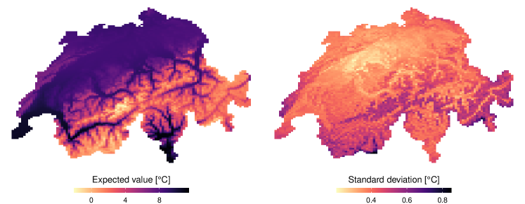
Figure 11: [Left] Expected mean temperature across Switzerland [Right] Standard deviation of mean temperature

Figure 12: [Left] Expected median temperature across Switzerland [Right] Standard deviation of median temperature

We insist on the fact that the quantiles estimations are done simultaneously as a by-product of the SLGP models. To illustrate this, we show the behaviour of these quantiles of daily mean temperature across a slice of Switzerland in Figure 13

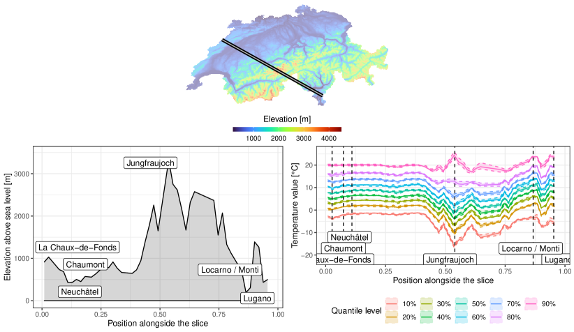
Figure 13: [Top] MAP of Switzerland and slice considered. [Bottom left] Elevation alongside the slice and Stations location. [Bottom right] Simultaneous quantile prediction (mean value and 10% quantile- 90% quantile bands) across a slice of Switzerland

References

- [1] {barticle}[author] \bauthor\bsnmAitchison, \bfnmJohn\binitsJ. (\byear1982). \btitleThe statistical analysis of compositional data. \bjournalJournal of the Royal Statistical Society: Series B (Methodological) \bvolume44 \bpages139–160. \endbibitem
- [2] {bbook}[author] \bauthor\bsnmAkhiezer, \bfnmNaum I.\binitsN. I. and \bauthor\bsnmGlazman, \bfnmIzrail M.\binitsI. M. (\byear2013). \btitleTheory of linear operators in Hilbert space. \bpublisherCourier Corporation. \endbibitem
- [3] {bbook}[author] \bauthor\bsnmAzaïs, \bfnmJean-Marc\binitsJ.-M. and \bauthor\bsnmWschebor, \bfnmMario\binitsM. (\byear2009). \btitleLevel sets and extrema of random processes and fields. \bpublisherJohn Wiley & Sons. \endbibitem
- [4] {barticle}[author] \bauthor\bsnmBect, \bfnmJulien\binitsJ., \bauthor\bsnmBachoc, \bfnmFrançois\binitsF. and \bauthor\bsnmGinsbourger, \bfnmDavid\binitsD. (\byear2019). \btitleA supermartingale approach to Gaussian process based sequential design of experiments. \bjournalBernoulli \bvolume25 \bpages2883–2919. \endbibitem
- [5] {barticle}[author] \bauthor\bsnmChung, \bfnmYeonseung\binitsY. and \bauthor\bsnmDunson, \bfnmDavid B\binitsD. B. (\byear2009). \btitleNonparametric Bayes conditional distribution modeling with variable selection. \bjournalJournal of the American Statistical Association \bvolume104 \bpages1646–1660. \endbibitem
- [6] {barticle}[author] \bauthor\bsnmCotter, \bfnmS. L.\binitsS. L., \bauthor\bsnmRoberts, \bfnmG. O.\binitsG. O., \bauthor\bsnmStuart, \bfnmA. M.\binitsA. M. and \bauthor\bsnmWhite, \bfnmD.\binitsD. (\byear2013). \btitleMCMC Methods for Functions: Modifying Old Algorithms to Make Them Faster. \bjournalStatistical Science \bvolume28 \bpages424–446. \bdoi10.1214/13-sts421 \endbibitem
- [7] {bbook}[author] \bauthor\bsnmCressie, \bfnmNoel\binitsN. (\byear1993). \btitleStatistics for spatial data. \bpublisherJohn Wiley & Sons. \endbibitem
- [8] {barticle}[author] \bauthor\bsnmDonner, \bfnmChristian\binitsC. and \bauthor\bsnmOpper, \bfnmManfred\binitsM. (\byear2018). \btitleEfficient bayesian inference for a gaussian process density model. \bjournalarXiv preprint arXiv:1805.11494. \endbibitem
- [9] {barticle}[author] \bauthor\bsnmDudley, \bfnmRichard M\binitsR. M. (\byear1967). \btitleThe sizes of compact subsets of Hilbert space and continuity of Gaussian processes. \bjournalJournal of Functional Analysis \bvolume1 \bpages290–330. \endbibitem
- [10] {barticle}[author] \bauthor\bsnmDunson, \bfnmDavid B\binitsD. B. and \bauthor\bsnmPark, \bfnmJu-Hyun\binitsJ.-H. (\byear2008). \btitleKernel stick-breaking processes. \bjournalBiometrika \bvolume95 \bpages307–323. \endbibitem
- [11] {barticle}[author] \bauthor\bsnmDunson, \bfnmDavid B\binitsD. B., \bauthor\bsnmPillai, \bfnmNatesh\binitsN. and \bauthor\bsnmPark, \bfnmJu-Hyun\binitsJ.-H. (\byear2007). \btitleBayesian density regression. \bjournalJournal of the Royal Statistical Society: Series B (Statistical Methodology) \bvolume69 \bpages163–183. \endbibitem
- [12] {barticle}[author] \bauthor\bsnmFan, \bfnmJianqing\binitsJ., \bauthor\bsnmYao, \bfnmQiwei\binitsQ. and \bauthor\bsnmTong, \bfnmHowell\binitsH. (\byear1996). \btitleEstimation of conditional densities and sensitivity measures in nonlinear dynamical systems. \bjournalBiometrika \bvolume83 \bpages189–206. \endbibitem
- [13] {barticle}[author] \bauthor\bsnmFan, \bfnmJianqing\binitsJ. and \bauthor\bsnmYim, \bfnmTsz Ho\binitsT. H. (\byear2004). \btitleA crossvalidation method for estimating conditional densities. \bjournalBiometrika \bvolume91 \bpages819–834. \endbibitem
- [14] {binproceedings}[author] \bauthor\bsnmGautier, \bfnmAthénaïs\binitsA., \bauthor\bsnmGinsbourger, \bfnmDavid\binitsD. and \bauthor\bsnmPirot, \bfnmGuillaume\binitsG. (\byear2020). \btitleProbabilistic ABC with Spatial Logistic Gaussian Process modelling. In \bbooktitleThird Workshop on Machine Learning and the Physical Sciences. \endbibitem
- [15] {barticle}[author] \bauthor\bsnmGautier, \bfnmAthénaïs\binitsA., \bauthor\bsnmGinsbourger, \bfnmDavid\binitsD. and \bauthor\bsnmPirot, \bfnmGuillaume\binitsG. (\byear2021). \btitleGoal-oriented adaptive sampling under random field modelling of response probability distributions. \bjournalESAIM: ProcS \bvolume71 \bpages89-100. \bdoi10.1051/proc/202171108 \endbibitem
- [16] {bbook}[author] \bauthor\bsnmGihman, \bfnmIosif Il’ich\binitsI. I. and \bauthor\bsnmSkorohod, \bfnmAnatolij Vladimirovič\binitsA. V. (\byear1974). \btitleThe theory of stochastic processes I. \bpublisherSpringer, Berlin, Heidelberg, New York. \endbibitem
- [17] {barticle}[author] \bauthor\bsnmGriffin, \bfnmJim E\binitsJ. E. and \bauthor\bsnmSteel, \bfnmMF J\binitsM. J. (\byear2006). \btitleOrder-based dependent Dirichlet processes. \bjournalJournal of the American statistical Association \bvolume101 \bpages179–194. \endbibitem
- [18] {barticle}[author] \bauthor\bsnmHairer, \bfnmMartin\binitsM. (\byear2009). \btitleAn introduction to stochastic PDEs. \bjournalLecture notes and arXiv:0907.4178. \endbibitem
- [19] {barticle}[author] \bauthor\bsnmHall, \bfnmPeter\binitsP., \bauthor\bsnmWolff, \bfnmRodney CL\binitsR. C. and \bauthor\bsnmYao, \bfnmQiwei\binitsQ. (\byear1999). \btitleMethods for estimating a conditional distribution function. \bjournalJournal of the American Statistical association \bvolume94 \bpages154–163. \endbibitem
- [20] {bphdthesis}[author] \bauthor\bsnmHenao, \bfnmRamon Giraldo\binitsR. G. (\byear2009). \btitleGeostatistical analysis of functional data, \btypePhD thesis, \bpublisherPh. D. thesis, Universitat Politecnica de Catalunya. \endbibitem
- [21] {barticle}[author] \bauthor\bsnmJain, \bfnmSonia\binitsS. and \bauthor\bsnmNeal, \bfnmRadford M\binitsR. M. (\byear2004). \btitleA split-merge Markov chain Monte Carlo procedure for the Dirichlet process mixture model. \bjournalJournal of computational and Graphical Statistics \bvolume13 \bpages158–182. \endbibitem
- [22] {barticle}[author] \bauthor\bsnmJara, \bfnmAlejandro\binitsA. and \bauthor\bsnmHanson, \bfnmTimothy E\binitsT. E. (\byear2011). \btitleA class of mixtures of dependent tail-free processes. \bjournalBiometrika \bvolume98 \bpages553–566. \endbibitem
- [23] {bbook}[author] \bauthor\bsnmKallenberg, \bfnmOlav\binitsO. (\byear2017). \btitleRandom measures, theory and applications \bvolume1. \bpublisherSpringer. \endbibitem
- [24] {barticle}[author] \bauthor\bsnmKleijn, \bfnmB. J. K.\binitsB. J. K. and \bauthor\bparticlevan der \bsnmVaart, \bfnmA. W.\binitsA. W. (\byear2006). \btitleMisspecification in infinite-dimensional Bayesian statistics. \bjournalThe Annals of Statistics \bvolume34 \bpages837 – 877. \bdoi10.1214/009053606000000029 \endbibitem
- [25] {barticle}[author] \bauthor\bsnmLenk, \bfnmPeter J.\binitsP. J. (\byear1988). \btitleThe logistic normal distribution for Bayesian, nonparametric, predictive densities. \bjournalJournal of the American Statistical Association \bvolume83 \bpages509–516. \endbibitem
- [26] {barticle}[author] \bauthor\bsnmLenk, \bfnmPeter J.\binitsP. J. (\byear1991). \btitleTowards a practicable Bayesian nonparametric density estimator. \bjournalBiometrika \bvolume78 \bpages531–543. \endbibitem
- [27] {barticle}[author] \bauthor\bsnmLeonard, \bfnmTom\binitsT. (\byear1978). \btitleDensity estimation, stochastic processes and prior information. \bjournalJournal of the Royal Statistical Society, Series B: Methodological \bvolume40 \bpages113–132. \endbibitem
- [28] {barticle}[author] \bauthor\bsnmMatheron, \bfnmGeorges\binitsG. (\byear1963). \btitlePrinciples of geostatistics. \bjournalEconomic Geology \bvolume58 \bpages1246-1266. \bdoi10.2113/gsecongeo.58.8.1246 \endbibitem
- [29] {bphdthesis}[author] \bauthor\bsnmMinka, \bfnmThomas Peter\binitsT. P. (\byear2001). \btitleA family of algorithms for approximate Bayesian inference, \btypePhD thesis, \bpublisherMassachusetts Institute of Technology. \endbibitem
- [30] {barticle}[author] \bauthor\bsnmNerini, \bfnmDavid\binitsD., \bauthor\bsnmMonestiez, \bfnmPascal\binitsP. and \bauthor\bsnmManté, \bfnmClaude\binitsC. (\byear2010). \btitleCokriging for spatial functional data. \bjournalJournal of Multivariate Analysis \bvolume101 \bpages409–418. \endbibitem
- [31] {bmisc}[author] \bauthor\bparticleof \bsnmMeteorology, \bfnmSwiss Federal Office\binitsS. F. O. and \bauthor\bsnmMeteoSwiss, \bfnmClimatology\binitsC. (\byear2019). \btitleClimatological Network - Daily Values. \bnoteAccessed on 01.10.2021. \endbibitem
- [32] {bmisc}[author] \bauthor\bparticleof \bsnmTopography swisstopo, \bfnmSwiss Federal Office\binitsS. F. O. (\byear2019). \btitleThe digital height model of Switzerland with a 200m grid. \bnoteAccessed on 01.10.2021. \endbibitem
- [33] {barticle}[author] \bauthor\bsnmPapaspiliopoulos, \bfnmOmiros\binitsO. and \bauthor\bsnmRoberts, \bfnmGareth O\binitsG. O. (\byear2008). \btitleRetrospective Markov chain Monte Carlo methods for Dirichlet process hierarchical models. \bjournalBiometrika \bvolume95 \bpages169–186. \endbibitem
- [34] {barticle}[author] \bauthor\bsnmPati, \bfnmDebdeep\binitsD., \bauthor\bsnmDunson, \bfnmDavid B\binitsD. B. and \bauthor\bsnmTokdar, \bfnmSurya T\binitsS. T. (\byear2013). \btitlePosterior consistency in conditional distribution estimation. \bjournalJournal of multivariate analysis \bvolume116 \bpages456–472. \endbibitem
- [35] {bbook}[author] \bauthor\bsnmPawlowsky-Glahn, \bfnmVera\binitsV. and \bauthor\bsnmBuccianti, \bfnmAntonella\binitsA. (\byear2011). \btitleCompositional data analysis: Theory and applications. \bpublisherJohn Wiley & Sons. \endbibitem
- [36] {binproceedings}[author] \bauthor\bsnmRahimi, \bfnmAli\binitsA. and \bauthor\bsnmRecht, \bfnmBenjamin\binitsB. (\byear2008). \btitleRandom features for large-scale kernel machines. In \bbooktitleAdvances in neural information processing systems \bpages1177–1184. \endbibitem
- [37] {binproceedings}[author] \bauthor\bsnmRahimi, \bfnmAli\binitsA. and \bauthor\bsnmRecht, \bfnmBenjamin\binitsB. (\byear2009). \btitleWeighted sums of random kitchen sinks: Replacing minimization with randomization in learning. In \bbooktitleAdvances in neural information processing systems \bpages1313–1320. \endbibitem
- [38] {barticle}[author] \bauthor\bsnmRamsay, \bfnmJames O\binitsJ. O. (\byear2004). \btitleFunctional data analysis. \bjournalEncyclopedia of Statistical Sciences \bvolume4. \endbibitem
- [39] {bmisc}[author] \bauthor\bsnmRojas, \bfnmAlex L\binitsA. L., \bauthor\bsnmGenovese, \bfnmChristopher R\binitsC. R., \bauthor\bsnmMiller, \bfnmChristopher J\binitsC. J., \bauthor\bsnmNichol, \bfnmRobert\binitsR. and \bauthor\bsnmWasserman, \bfnmLarry\binitsL. (\byear2005). \btitleConditional density estimation using finite mixture models with an application to astrophysics. \endbibitem
- [40] {bphdthesis}[author] \bauthor\bsnmScheuerer, \bfnmMichael\binitsM. (\byear2009). \btitleA comparison of models and methods for spatial interpolation in statistics and numerical analysis, \btypePhD thesis, \bpublisherNiedersächsische Staats-und Universitätsbibliothek Göttingen. \endbibitem
- [41] {barticle}[author] \bauthor\bsnmSchwartz, \bfnmLorraine\binitsL. (\byear1965). \btitleOn bayes procedures. \bjournalZeitschrift für Wahrscheinlichkeitstheorie und verwandte Gebiete \bvolume4 \bpages10–26. \endbibitem
- [42] {bbook}[author] \bauthor\bsnmStein, \bfnmMichael L\binitsM. L. (\byear2012). \btitleInterpolation of spatial data: some theory for kriging. \bpublisherSpringer Science & Business Media. \endbibitem
- [43] {barticle}[author] \bauthor\bsnmTokdar, \bfnmSurya T\binitsS. T. (\byear2007). \btitleTowards a faster implementation of density estimation with logistic Gaussian process priors. \bjournalJournal of Computational and Graphical Statistics \bvolume16 \bpages633–655. \endbibitem
- [44] {barticle}[author] \bauthor\bsnmTokdar, \bfnmSurya T\binitsS. T. and \bauthor\bsnmGhosh, \bfnmJayanta K\binitsJ. K. (\byear2007). \btitlePosterior consistency of logistic Gaussian process priors in density estimation. \bjournalJournal of statistical planning and inference \bvolume137 \bpages34–42. \endbibitem
- [45] {barticle}[author] \bauthor\bsnmTokdar, \bfnmSurya T\binitsS. T., \bauthor\bsnmZhu, \bfnmYu M\binitsY. M. and \bauthor\bsnmGhosh, \bfnmJayanta K\binitsJ. K. (\byear2010). \btitleBayesian density regression with logistic Gaussian process and subspace projection. \bjournalBayesian analysis \bvolume5 \bpages319–344. \endbibitem
- [46] {barticle}[author] \bauthor\bsnmTrippa, \bfnmLorenzo\binitsL., \bauthor\bsnmMüller, \bfnmPeter\binitsP. and \bauthor\bsnmJohnson, \bfnmWesley\binitsW. (\byear2011). \btitleThe multivariate beta process and an extension of the Polya tree model. \bjournalBiometrika \bvolume98 \bpages17–34. \endbibitem
- [47] {barticle}[author] \bauthor\bparticlevan der \bsnmVaart, \bfnmAad W\binitsA. W. and \bauthor\bparticlevan \bsnmZanten, \bfnmJ Harry\binitsJ. H. (\byear2008). \btitleRates of contraction of posterior distributions based on Gaussian process priors. \bjournalThe Annals of Statistics \bvolume36 \bpages1435–1463. \endbibitem
- [48] {barticle}[author] \bauthor\bsnmWalker, \bfnmStephen G\binitsS. G. (\byear2007). \btitleSampling the Dirichlet mixture model with slices. \bjournalCommunications in Statistics—Simulation and Computation® \bvolume36 \bpages45–54. \endbibitem
- [49] {barticle}[author] \bauthor\bsnmZhu, \bfnmXujia\binitsX. and \bauthor\bsnmSudret, \bfnmBruno\binitsB. (\byear2020). \btitleEmulation of stochastic simulators using generalized lambda models. \bjournalarXiv preprint arXiv:2007.00996. \endbibitem