Improving Generalization of Deep Reinforcement Learning-based TSP Solvers

Abstract

Recent work applying deep reinforcement learning (DRL) to solve traveling salesman problems (TSP) has shown that DRL-based solvers can be fast and competitive with TSP heuristics for small instances, but do not generalize well to larger instances. In this work, we propose a novel approach named MAGIC that includes a deep learning architecture and a DRL training method. Our architecture, which integrates a multilayer perceptron, a graph neural network, and an attention model, defines a stochastic policy that sequentially generates a TSP solution. Our training method includes several innovations: (1) we interleave DRL policy gradient updates with local search (using a new local search technique), (2) we use a novel simple baseline, and (3) we apply curriculum learning. Finally, we empirically demonstrate that MAGIC is superior to other DRL-based methods on random TSP instances, both in terms of performance and generalizability. Moreover, our method compares favorably against TSP heuristics and other state-of-the-art approach in terms of performance and computational time.

I Introduction

Traveling Salesman Problem (TSP) is one of the most famous combinatorial optimization problems. Given the coordinates of some points, the goal in the TSP problem is to find a shortest tour that visits each point exactly once and returns to the starting point. TSP is an NP- hard problem [20] , even in its symmetric 2D Euclidean version, which is this paper’s focus. Traditional approaches to solve TSP can be classified as exact or heuristic. Exact solvers, such as Concorde [2] or based on integer linear programming, can find an optimal solution. However, since TSP is NP- hard, such algorithms have computational times that increase exponentially with the size of a TSP instance. In contrast, heuristic approaches provide a TSP solution with a much shorter computational time compared to exact solvers , but do not guarantee optimality. These approaches are either constructive (e.g., farthest insertion [17]), perturbative (e.g., 2-opt [1], LKH [13]), or hybrid. However, they may not provide any good performance guarantee and are still computationally costly. Indeed, even a quadratic computational complexity may become prohibitive when dealing with large TSP instances (e.g., 1000 cities).

Thus, recent research work has focused on using Deep Learning (DL) to design faster heuristics to solve TSP problems. Since training on large TSP instances is costly, generalization is a key factor in such DL-based approaches. They are either based on Supervised Learning (SL) [24, 16, 12] or Reinforcement Learning (RL) [6, 17, 18, 8]. These different approaches , which are either constructive, perturbative, or hybrid, have different pros and cons. For example, [12]’s model , which combines DL with Monte Carlo Tree Search (MCTS) [9], has great generalization capabilities. Namely, they can train on small TSP instances and perform well on larger instances. However, the computational cost of [12]’s model is high due to MCTS. In contrast, other models (e.g., [16, 17]) can solve small TSP instances with fast speed and great performance, but they lack generalizability.

In this paper, we propose a novel deep RL approach that can achieve excellent performance with good generalizability for a reasonable computational cost. The contributions of this paper can be summarized as follows. Our approach is based on an encoder-decoder model (using Graph Neural Network (GNN) [5] and Multilayer Perceptron (MLP) [19] as the encoder and an attention mechanism [23] as the decoder), which is trained with a new deep RL method that interleaves policy gradient updates (with a simple baseline called policy rollout baseline) and local search (with a novel combined local search technique). Moreover, curriculum learning is applied to help with training and generalization. Due to all the used techniques, we name our model as MAGIC (MLP for M, Attention for A, GNN for G, Interleaved local search for I, and Curriculum Learning for C). Finally, we empirically show that MAGIC is a state-of-the-art deep RL solver for TSP, which offers a good trade-off in terms of performance, generalizability, and computational time.

This paper is structured as follows. Section II overviews related work. Section III recalls the necessary background. Section IV introduces our model architecture. Section V describes our novel training technique by explaining how we apply local search, the policy rollout baseline, and curriculum learning during training. Section VI presents the experimental results and Section VII concludes.

II Related Work

RL can be used as a constructive heuristic to generate a tour or as a machine learning method integrated in a traditional method, such as [8], which learns to apply 2-opt. For space reasons, we mainly discuss deep RL work in the constructive approach (see [4] for a more comprehensive survey), since they are the most related to our work. Besides, a recent work [15] suggests that RL training may lead to better generalization than supervised learning.

Such deep RL work started with Pointer Network [24] , which was proposed as a general model that could solve an entire class of TSP instances. It has an encoder-decoder architecture, both based on recurrent neural networks, combined with an attention mechanism [3]. The model is trained in a supervised way using solutions generated by Concorde [2]. The results are promising, but the authors focused only on small-scale TSP instances ( with up to 50 cities) and did not deal with generalization.

This approach was extended to the RL setting [6] and shown to scale to TSP with up to 100 cities. The RL training is based on an actor-critic scheme using tour lengths as unbiased estimates of the value of a policy. In contrast to [6], a value-based deep RL [10] was also investigated to solve graph combinatorial optimization problems in general and TSP in particular. The approach uses graph embeddings to represent partial solutions and RL to learn a greedy policy.

The Attention Model [17] improves the Pointer Network [24] notably by replacing the recurrent neural networks by attention models [23] and using RL training with a simple greedy rollout baseline. These changes allowed them to achieve better results on small-scale TSP instances, as well as to generalize to 100-city TSP instances. However, their model fails to generalize well to large-scale TSP (e.g., with 1000 cities) and their algorithm does not scale well in terms of memory usage.

A similar, although slightly more complex, approach is proposed in [11], which also suggests to improve the tour returned by the deep RL policy with a 2-opt local search, which makes the overall combination a hybrid heuristics. In contrast to that work, we not only apply local search as a final improvement step, but also integrate local search in the training of our deep RL model. Moreover, we use a more sophisticated local search.

Moreover, the Graph Pointer Network (GPN) model [18] was proposed to improve over previous models by exploiting graph neural networks [5] and using a central self-critic baseline, which is a centered greedy rollout baseline. Like [11], 2-opt is also considered. As a result, they report good results when generalizing to large-scale TSP instances. Our simpler model and new training method outperforms GPN on both small and larger TSP instances.

III Background

This section provides the necessary information to understand our model architecture (Section IV) and our training method (Section V). For any $n\in\mathbb{N}$, $[n]$ denotes $\{1,2,\ldots,n\}$. Vectors and matrices are denoted in bold.

III-A Traveling Salesman Problem

A Traveling Salesperson Problem (TSP) can informally be stated as follows. Given $N$ cities, the goal in a TSP instance is to find a shortest tour that visits each city exactly once. Formally, the set of $N$ cities can be identified to the set $[N]=\{1,2,\ldots,N\}$. In the symmetric 2D Euclidean version of the TSP problem, each city $i\in[N]$ is characterized by its 2D-coordinates $\bm{x}_{i}\in\mathbb{R}^{2}$. Let $X$ denote the set of city coordinates $\{\bm{x}_{i}\mid i\in[N]\}$ and $\bm{X}\in\mathbb{R}^{N\times 2}$ the matrix containing all these coordinates. The distance $d_{ij}$ between two cities $(i,j)\in[N]^{2}$ is usually measured in terms of the L2-norm $\|\cdot\|_{2}$:

$$d_{ij}=d_{ji}=\|\bm{x}_{i}-\bm{x}_{j}\|_{2}.$$ (1)

A feasible TSP solution, called a tour, corresponds to a permutation $\sigma$ over $[N]$. Its length is defined as:

$$\begin{split}L_{\sigma}(X)&=\sum_{t=1}^{N}d_{\sigma(t)\sigma(t+1)}=\sum_{t=1}^{N}\|\bm{x}_{\sigma(t)}-\bm{x}_{\sigma(t+1)}||_{2}\end{split}$$ (2)

where for $t\in[N]$, $\sigma(t)\in[N]$ is the $t$-th city visited in the tour defined by $\sigma$, and by abuse of notation, $\sigma(N+1)=\sigma(1)$. Therefore, the TSP problem can be viewed as the following optimization problem:

$$\begin{split}\min_{\sigma}L_{\sigma}(X)=\min_{\sigma}\sum_{t=1}^{N}\|\bm{x}_{\sigma(t)}-\bm{x}_{\sigma(t+1)}\|_{2}.\end{split}$$ (3)

Since scaling the city positions does not change the TSP solution, we assume in the remaining of the paper that the coordinates of all cities are in the square $[0,1]^{2}$, as done in previous work [6, 8, 17, 18].

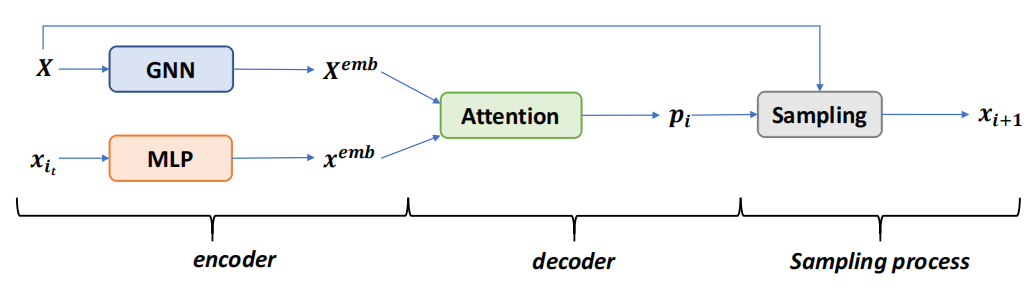
Figure 1: Architecture of the model used in MAGIC.

III-B Insertion heuristic s and k-opt optimization for TSP

Since TSP is an NP-hard problem [20], various heuristic techniques have been proposed to quickly compute a solution, which may however be sub-optimal. We recall two family of heuristics: insertion heuristics [17] and k-opt [7].

Insertion heuristics (including nearest, farthest , and random insertion) are constructive, i.e., they iteratively build a solution. They work as follows. They first randomly choose a starting city and repeatedly insert one new city at a time until obtaining a complete tour. Let $\hat{\sigma}$ denote a partial tour, i.e., a partial list of all cities. Different insertion heuristics follow different rule s to choose a new city $\ell$: random insertion choose s a new city $\ell$ randomly; nearest insertion chooses according to:

$$\ell=\arg\min_{j\notin\hat{\sigma}}\min_{i\in\hat{\sigma}}d_{ij},$$ (4)

and farthest insertion chooses according to the following rule:

$$\ell=\arg\max_{j\notin\hat{\sigma}}\min_{i\in\hat{\sigma}}d_{ij}$$ (5)

where $j\not\in\hat{\sigma}$ means city $j$ is not in the partial tour $\hat{\sigma}$ and $i\in\hat{\sigma}$ means city $i$ is in the partial tour. The position $t$ where city $\ell$ is inserted into ${\color[rgb]{0,0,0}\hat{\sigma}}$ is determined such that: $d_{\hat{\sigma}(t)\ell}+d_{\ell\hat{\sigma}(t+1)}-d_{{\color[rgb]{0,0,0}\hat{\sigma}(t)}\hat{\sigma}(t+1)}$ is minimized.

A classic local search heuristic is $k$-opt, which aims to improve an exist ing tour $\sigma$ by swapping $k$ chosen edge s at each iteration. The simplest one is $2$-opt, which can replace $\sigma=\big{(}\sigma(1),\sigma(2)...,\sigma({\color[rgb]{0,0,0}i}),...,\sigma({\color[rgb]{0,0,0}j}),...,\sigma(N)\big{)}$ by $\sigma^{\prime}=\big{(}\sigma(1),...,\sigma({\color[rgb]{0,0,0}i}),\sigma({\color[rgb]{0,0,0}j}),\sigma({\color[rgb]{0,0,0}j}-1),...,\sigma({\color[rgb]{0,0,0}i}+1),\sigma({\color[rgb]{0,0,0}j}+1),...,\sigma(N)\big{)}$ where ${\color[rgb]{0,0,0}i}<{\color[rgb]{0,0,0}j}<N$ if $L_{\sigma^{\prime}}(X)<L_{\sigma}(X)$. This kind improvement can be found in different ways. For instance, traditional 2-opt may examine all pairs of edges, while random 2-opt examines randomly-selected pairs. LKH [13] is one algorithm that applies $k$-opt and achieve s nearly optimal results. However, LKH has a long run time, especially for large-scale TSP problems.

IV Model and Architecture

RL can be used as a constructive method to iteratively generate a complete tour: at each iteration $t$, a new city $a_{t}$ with coordinates $\bm{x}_{a_{t}}$ is selected based on the list of previously selected cities and the description of the TSP instance. Formally, this RL model is defined as follows. A state $\bm{s}_{t}$ is composed of the TSP description and the sequence of already visited cities $(i_{1},i_{2},\ldots,i_{t-1})$ at time step $t$. State $s_{1}$ denotes the initial state where no city has been selected yet and state $s_{N+1}$ represents the state where the whole tour has already been constructed. An action $a_{t}\in[N]$ corresponds to the next city $i_{t}$ to be visited, i.e., $a_{t}=i_{t}$. This RL problem corresponds to a repeated $N$-horizon sequential decision-making problem where the action set for any time step depends on the current state and only contains the cities that have not been visited yet. The immediate reward for performing an action in a state is given as the negative length between the last visited city and the next chosen one:

$$r(\bm{s}_{t},a_{t})=\left\{\begin{array}[]{ll}0&\mbox{for }t=1\\ -d_{i_{t-1}i_{t}}&\mbox{for }t=2,\ldots,N\end{array}\right.$$ (6)

After choosing the first city, no reward can be computed yet. After the last city, a final additional reward is provided given by $r(\bm{s}_{N+1})=-d_{i_{N}i_{1}}$. Thus, a complete trajectory corresponds to a tour and the return of a trajectory is equal to the negative the length of that tour. Most RL-based constructive solver is based on this RL formulation. In Section V, we change the return provided to the RL agent to improve its performance using local search.

To perform the selection of the next city, we propose the MAGIC architecture (see Fig. 1), which corresponds to a stochastic policy (see Section V for more details). It is composed of three parts: (A) an encoder implemented with a graph neural network (GNN) [5] and a multilayer perceptron (MLP), (B) a decoder based on an attention mechanism [23], and (C) a sampling process.

IV-A Encoder

When solving a TSP problem, not only should the last selected city be considered, but also the whole city list should be taken into account as background information. Since the information contained in 2D coordinates is limited and does not include the topology of the cities, we leverage GNN and MLP to encode city coordinates into a higher dimensional space, depicted in Fig. 1. The GNN is used to encode the city coordinates $\bm{X}\in\mathbb{R}^{N\times 2}$ into $\bm{X}^{emb}\in\mathbb{R}^{N\times H}$ where $H$ is the dimension of the embedding space. The MLP is used to encode the last selected city $\bm{x}_{i_{t}}\in X$ at iteration $t\in[N]$ into $\bm{x}^{emb}\in\mathbb{R}^{H}$. Therefore, generally speaking, the GNN and MLP in MAGIC can be viewed as two functions:

$$\text{GNN}:\mathbb{R}^{N\times 2}\rightarrow\mathbb{R}^{N\times H},\ \text{MLP}:\mathbb{R}^{2}\rightarrow\mathbb{R}^{H}.$$ (7)

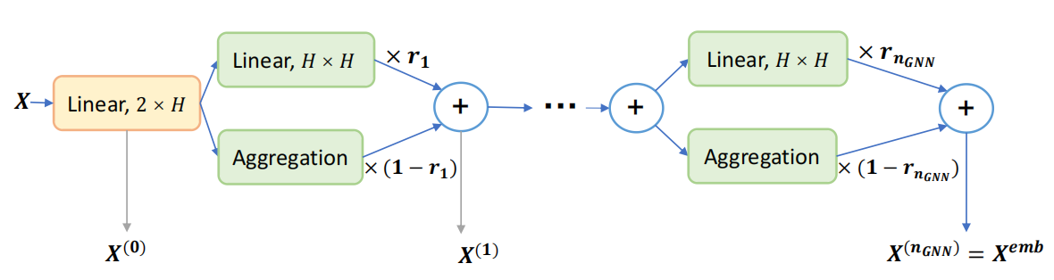
Figure 2: Detailed Architecture of GNN.

IV-A1 GNN

GNN is a technique which can embed all nodes in a graph together. Similarly to the GPN model [18], we use a GNN to encode the whole city list of a TSP instance. Fig. 2 shows the detailed architecture of the GNN used in MAGIC. After $\bm{X}\in\mathbb{R}^{N\times 2}$ is transformed into a vector $\bm{X}^{(0)}\in\mathbb{R}^{N\times H}$, $\bm{X}^{(0)}$ will go through $n_{\text{GNN}}$ layers of GNN. Each layer of GNN can be expressed as

$$\bm{X}^{(t)}=r\cdot\bm{X}^{(t-1)}\bm{\Theta}^{(t)}+(1-r)\cdot\mathrm{F}^{(t)}\left(\frac{\bm{X}^{(t-1)}}{N-1}\right)$$ (8)

where $\bm{X}^{(t-1)}\in\mathbb{R}^{N\times H}$ is the input of the $t^{th}$ layer of the GNN for $t\in[n_{\text{GNN}}]$, $\bm{X}^{(n_{\text{GNN}})}=\bm{X}^{emb}$, $\bm{\Theta}^{(t)}$ is an $H\times H$ learnable matrix, which is represented by a neural network, $\mathrm{F}^{(t)}:\mathbb{R}^{N\times H}\rightarrow\mathbb{R}^{N\times H}$ is the aggregation function [5] , and ${\color[rgb]{0,0,0}r\in[0,1]}$ is a trainable parameter.

IV-A2 MLP

While the GNN provides us with general information within the whole city list $X$ , we also need to encode the last selected city $\bm{x}_{i_{t}}\in\mathbb{R}^{2}$. In contrast to previous work using complex architectures like GNN or LSTM [14], we simply use an MLP. Using a GNN would make the embedding of the last selected city depend on the whole city list included the already-visited cities, while using an LSTM would make the embedding depends on the order of visited cities, which is in fact irrelevant.

IV-B Decoder

The decoder of the MAGIC model is based on an attention mechanism , which was also used in several previous studies [6, 17, 18, 12]. The output of the decoder is a pointer vector $\bm{u}^{(t)}\in\mathbb{R}^{N}$ [6], which can be expressed as:

$$\bm{u}^{(t)}_{j}=\begin{cases}-\infty\text{\ \ \ \ \ \ \ \ \ if}\,\,\exists\,k\leq t\text{,}\,\,i_{k}=j&\\ \bm{w}\cdot\tanh\left(\bm{X}^{emb}_{j}\bm{\Theta}_{g}+\bm{\Theta}_{m}\bm{x}^{emb}\right)\text{ otherwise}&\end{cases}$$ (9)

where ${\bm{u}}^{(t)}_{j}$ is the $j^{th}$ entry of the vector ${\bm{u}}^{(t)}$, $\bm{X}^{emb}_{j}$ is the $j^{th}$ row of the matrix $\bm{X}^{emb}$, $\bm{\Theta}_{g}$ and $\bm{\Theta}_{m}$ are trainable matrices with shape $H\times H$, $\bm{w}\in\mathbb{R}^{N}$ is a trainable weight vector. For the definitions of $\bm{X}^{emb}$ and $\bm{x}^{emb}$, please refer to Fig. 1.

A softmax transformation is used to turn $\bm{u}^{(t)}$ into a probability distribution $\bm{p}^{(t)}=\big{(}{\bm{p}}^{(t)}_{j}\big{)}_{j\in[N]}$ over cities:

$$\bm{p}^{(t)}=\mathrm{softmax}(\bm{u}^{(t)})=\left(\frac{e^{\bm{u}^{(t)}_{j}}}{\sum_{j=1}^{N}e^{\bm{u}^{(t)}_{j}}}\right)_{j\in[N]}$$ (10)

where ${\bm{p}}^{(t)}_{j}$ is the $j^{th}$ entry of the probability distribution ${\bm{p}}^{(t)}$ and ${\bm{u}}^{(t)}_{j}$ is the $j^{th}$ entry of the vector ${\bm{u}}^{(t)}$. Notice that if the $j^{th}$ city is visited, then ${\bm{u}}^{(t)}_{j}=-\infty$ due to (9). Under this circumstance, ${\bm{p}}^{(t)}_{j}=0$ according to (10). That is to say, all visited cities cannot be visited again.

IV-C Sampling Process

After we obtain the probability distribution ${\bm{p}}^{(t)}$, it is trivial to select the next city. Indeed, ${\bm{p}}^{(t)}$ corresponds to the RL policy $\pi_{\bm{\theta}}$ at time step $t$:

$$\pi_{\bm{\theta}}(a_{t}\mid\bm{s}_{t})=\bm{p}^{(t)}_{a_{t}}$$ (11)

where $\bm{s}_{t}$ (resp. $a_{t}$) is the state (resp. action) at time step $t$ and $\bm{p}^{(t)}_{a_{t}}$ is the probability of choosing $a_{t}$ as the $t^{th}$ city. Therefore, we just need to sample the next city according to the probability distribution ${\bm{p}}^{(t)}$.

V Algorithm and Training

For the training of MAGIC, we propose to interleave standard policy gradient updates with local search. In contrast to previous work, our idea is to learn a policy that can generate tours that can be easily improved with local search. Next, we explain our local search technique, which include a novel local insertion-based heuristics. Then, we present how policy gradient with a simple policy rollout baseline can be applied. Finally, we motivate the use of stochastic curriculum learning method in our setting.

Algorithm 1 Local Insertion Optimization Algorithm

1:  Input: A set of city coordinates $X=\{\bm{x}_{i}\}_{i=1}^{N}$, current tour $\sigma$, and $\gamma\in[0,1]$

2:  Output: An improved tour $\sigma$

3:  for $t=1$ to $N$ do

4:     $t^{*}=\arg\min_{t^{\prime},\,\,|t^{\prime}-t|<\gamma\times N}L_{\sigma_{t,t^{\prime}}}(X)$

5:     $\sigma\leftarrow\sigma_{t,t^{*}}$

6:  end for

7:  return  $\sigma$

V-A Local search

We describe the local search technique that we use for training our model and to improve the tour output by the RL policy. Our technique uses two local search heuristics in combination: random opt and a local insertion heuristics, which is novel to the best of our knowledge. The two heuristics have been chosen and designed to be computationally efficient, which is important since we will apply them during RL training. The motivation for combining two heuristics is that when one method gets stuck in some local minimum, the other method may help escape from it.

For random 2-opt, we randomly pick 2 arcs for improvement and repeat for $\alpha\times N^{\beta}$, where $N$ is the number of the cities and $\alpha>0$ and $\beta\in\mathbb{R}$ are two hyperparameters. We set $\alpha$ and $\beta$ here to have a flexible control of the strength of this local search and make it stronger if needed for larger TSP problems. With this procedure, random 2-opt can be much faster than traditional 2-opt.

Inspired by the insertion heuristics, we propose local insertion optimization. Let $\sigma$ be the current tour and $\sigma_{t,t^{\prime}}=(\sigma(1),...,\sigma(t^{\prime}),\sigma(t),\sigma(t^{\prime}+1),...,\sigma(t-1),\sigma(t+1),...,\sigma(N))$ if $t^{\prime}\neq t-1$ and $\sigma_{t,t-1}=\sigma$. This method (see Algorithm 1) first iterates through all indices $t\in[N]$, and for each index $t$, we let $t^{*}=\arg\min_{t^{\prime},\,\,|t^{\prime}-t|<\gamma\times N}L_{\sigma_{t,t^{\prime}}}(X)$, where $\gamma\in[0,1]$ is a hyperparameter, and then replace $\sigma$ by $\sigma_{t,t^{*}}$. The rationale for restricting the optimization with hyperparameter $\gamma$ is as follows. For a good suboptimal tour $\sigma$, cities that are close in terms of visit order in $\sigma$ are usually also close in terms of distance. In that case, $\sigma_{t,t^{\prime}}$ is unlikely to improve over $\sigma$ when $t$ and $t^{\prime}$ are far apart. Thus, we set $\gamma$ to limit the search range to increase the computational efficiency of this heuristics.

We call our local search technique combined local search (see Algorithm 2), which applies random 2-opt followed by local insertion optimization repeatedly for $I$ times, where $I$ is a hyperparameter.

Algorithm 2 Combined Local Search Algorithm

1:  Input: A set of city coordinates $X=\{x_{i}\}_{i=1}^{N}$, current tour $\sigma$, hyperparameters $\alpha$, $\beta$, $\gamma$ and $I$ for local search.

2:  Output: An improved tour $\sigma$

3:  for $t=1$ to $I$ do

4:     for $t^{\prime}=1$ to $\alpha N^{\beta}$ do

5:        $\sigma\leftarrow$ apply random 2-opt on $\sigma$

6:     end for

7:     $\sigma\leftarrow$ apply Local Insertion Optimization$(X,\sigma,\gamma)$

8:  end for

9:  return  $\sigma$

V-B Interleaved RL training with the policy rollout baseline

Our model is trained with the REINFORCE [25] algorithm. The novelty is that we interleave local search with the policy gradient updates. When the current policy $\pi_{\bm{\theta}}$ outputs a tour $\sigma$, this solution is further improved with our combined local search technique to obtain a new tour $\sigma_{+}$. In contrast to previous work, this tour $\sigma_{+}$ instead of $\sigma$ is used to evaluate policy $\pi_{\bm{\theta}}$. The rationale for this procedure is to make the RL policy and local search work in synergy by favoring learning policies that generate tours that can be easily improved by the combined local search. If the RL training and local search are not coordinated, as done in previous work, then a trained policy may generate tours that are hard to improve by local search.

V-B1 Policy Gradient

We recall first standard policy gradient and then explain how we modify it. With the reward function in (6), the RL goal would be to find ${\bm{\theta}}^{\star}$ such that

$${\bm{\theta}}^{\star}=\arg\max_{\bm{\theta}}J(\bm{\theta})=\arg\max_{\bm{\theta}}\mathbb{E}_{{\color[rgb]{0,0,0}\tau\sim\bm{p}_{\bm{\theta}}(\tau)}}\left[\sum_{t=1}^{N+1}r_{t}\right],$$ (12)

where $r_{t}=r(\bm{s}_{t},a_{t})$ for $t\in[N]$, $r_{N+1}=r(\bm{s}_{N+1})$, $\tau=(\bm{s}_{1},a_{1},\bm{s}_{2},a_{2},\ldots,\bm{s}_{N},a_{N},\bm{s}_{N+1})$ is a trajectory, and $\bm{p}_{\bm{\theta}}$ is the probability distribution over tours induced by policy $\pi_{\bm{\theta}}$. Recall the gradient of $J(\theta)$ [25] is:

$$\nabla_{\bm{\theta}}J(\bm{\theta})=\mathbb{E}_{\tau}\left[\left(\sum_{t=1}^{N}\nabla_{\bm{\theta}}\log{\color[rgb]{0,0,0}\pi_{\bm{\theta}}}({a}_{t}|\bm{s}_{t})\right)\left(\sum_{t=1}^{N+1}r_{t}\right)\right]$$ (13)

where $\mathbb{E}_{\tau}$ stands for $\mathbb{E}_{{\color[rgb]{0,0,0}\tau\sim\bm{p}_{\bm{\theta}}(\tau)}}$. For a large enough batch $B$ of trajectories, (13) is approximated with the empirical mean:

$$J(\bm{\theta})\approx\hat{\mathbb{E}}_{B}\left[\sum_{t=1}^{N}r^{(b)}_{t}\right]=\frac{1}{|B|}\sum_{b=1}^{|B|}\sum_{t=1}^{N+1}r^{(b)}_{t}$$ (14)

where $r^{(b)}_{t}=r(\bm{s}^{(b)}_{t},{a}^{(b)}_{t})$, $\bm{s}^{(b)}_{t}$ (resp. ${a}^{(b)}_{t}$) is the state (resp. action) at time step $t$ of the $b$-th trajectory $\tau^{(b)}$ generated by $\pi_{\bm{\theta}}$, and $\hat{\mathbb{E}}_{B}$ denotes the empirical mean operation. Then the policy gradient in (13) can be approximated by:

$$\nabla_{\bm{\theta}}J(\bm{\theta})\!\approx\!\hat{\mathbb{E}}_{B}\left[\big{(}\sum_{t=1}^{N}\nabla_{\bm{\theta}}\log{\color[rgb]{0,0,0}\pi_{\bm{\theta}}}({a}^{(b)}_{t}|\bm{s}^{(b)}_{t})\big{)}\big{(}\sum_{t=1}^{N+1}r^{(b)}_{t}\big{)}\right]$$ (15)

Instead of updating $\bm{\theta}$ with this policy gradient, in our interleaved training, we use:

$$-\hat{\mathbb{E}}_{B}\left[\big{(}\sum_{t=1}^{N}\nabla_{\bm{\theta}}\log{\color[rgb]{0,0,0}\pi_{\bm{\theta}}}({a}^{(b)}_{t}|\bm{s}^{(b)}_{t})\big{)}L_{\sigma_{+}^{(b)}}(X)\right]$$ (16)

where $\sigma_{+}^{(b)}$ is the improved tour obtained from our combined local search from $\sigma^{(b)}$, the tour induced by trajectory $\tau^{(b)}\in B$. By construction, $L_{\sigma_{+}^{(b)}}(X)\leq L_{\sigma^{(b)}}(X)=-\sum_{t=1}^{N+1}r^{(b)}_{t}$.

V-B2 Policy rollout baseline

In order to reduce the variance of the policy gradient estimate (16), we use a simple baseline and update $\bm{\theta}$ in the following direction:

$$-\hat{\mathbb{E}}_{B}\left[\big{(}\sum_{i=1}^{N}\nabla_{\bm{\theta}}\log{\color[rgb]{0,0,0}\pi_{\bm{\theta}}}({a}^{(b)}_{t}|\bm{s}^{(b)}_{t})\big{)}\big{(}L_{\sigma_{+}^{(b)}}(X)-l^{(b)}\big{)}\right]$$ (17)

where $l^{(b)}=-L_{\sigma^{(b)}}(X)$ is the baseline, which we call the policy rollout baseline. Such a baseline gives more weight in the policy gradient when local search can make more improvement. In our experiments, our baseline performs better than the previous greedy baselines [17, 18] in our training process. One other nice feature of our baseline is that it does not incur any extra computation since $L_{\sigma^{(b)}}(X)$ is already computed when policy generates $\sigma^{(b)}$.

V-C Stochastic Curriculum Learning

Curriculum Learning (CL) is a widely-used technique in machine learning (and RL) [22], which can facilitate learning and improve generalization. Although it can be implemented in various ways, its basic principle is to control the increasing difficulty of the training instances.

To train MAGIC, we propose a stochastic CL technique where the probability of choosing harder instances increases over training steps. We choose the number of cities as a measure of difficulty for a TSP instance, which is assumed to be in $\{10,11,\ldots,50\}$ in our experiments. We explain next how this selection probability is defined.

For epoch $e$, we define the vector $\bm{g}^{(e)}\in\mathbb{R}^{41}$ (since there are 41 integers between 10 and 50) to be

$$\bm{g}^{(e)}_{k}=\frac{1}{\sqrt{2\pi}{\color[rgb]{0,0,0}\sigma_{\mathcal{N}}}}\exp^{-\frac{1}{2}\left(\frac{(k+10)-e}{\sigma_{\mathcal{N}}}\right)^{2}}$$ (18)

where $\bm{g}^{(e)}_{k}$ represents the $k^{th}$ entry of $\bm{g}^{(e)}$, and $\sigma_{\footnotesize{\mathcal{N}}}$ is a hyperparameter which represents the standard deviation of the normal distribution. Then, we use a softmax to formulate the probability distribution $\bm{p}^{(e)}$ of this epoch

$$\bm{p}^{(e)}=\text{softmax}(\bm{g}^{(e)})$$ (19)

where $\bm{p}^{(e)}\in[0,1]^{41}$, and the $k^{th}$ entry of $\bm{p}^{(e)}$ represents to probability of choosing TSP of $(k+10)$ cities at epoch $e$.

V-D Overall training process

In this part, we summarize our training process by providing the corresponding pseudo code in Algorithm 3.

Algorithm 3 REINFORCE with Stochastic CL, Policy Rollout Baseline and Combined local search

1:  Input: Total number of epochs $E$, training steps per epoch $T$, batch size $|B|$, hyperparameters $\alpha$, $\beta$, $\gamma$ and $I$ for local search

2:  Initialize $\bm{\theta}$

3:  for $e=1$ to $E$ do

4:     $N\leftarrow$ Sample from $\bm{p}^{(e)}$ according to Stochastic CL

5:     for $t=1$ to $T$ do

6:        $\forall{b\in\{1,...,|B|\}}\,X^{(b)}\,\leftarrow$ Random TSP instance with $N$ cities

7:        $\forall{b\in\{1,...,|B|\}}\,\sigma^{(b)}\,\leftarrow$ Apply $\pi_{\bm{\theta}}$ on $X^{(b)}$

8:        $\forall{b\in\{1,...,|B|\}}\,\sigma_{+}^{(b)}\,\leftarrow$ Apply the combined local search on $\sigma^{(b)}$

9:        Compute gradient in (17) using $\sigma^{(b)}$ and $\sigma_{+}^{(b)}$

10:        $\bm{\theta}\leftarrow$ Update in the direction of this gradient

11:     end for

12:  end for

Notice that line  7 can be replaced by any model that can used to generate a tour, showing that a variety of models can fit in our training process to improve their performance for TSP problems.

VI Experiment s

TABLE I: Results and comparisons on small TSP cases, obtained by testing on 10,000 instances for TSP 20, 50 and 100

Method	Type	TSP20			TSP50			TSP100
		Length	Gap	Time(s)	Length	Gap	Time(s)	Length	Gap	Time(s)
Concorde∗	Exact Solver	3.830	0.00%	138.6	5.691	0.00%	820.8	7.761	0.00%	3744
Gurobi∗	Exact Solver	3.830	0.00%	139.8	5.691	0.00%	1572	7.761	0.00%	12852
2-opt	Heuristic	4.082	6.56%	0.33	6.444	13.24%	2.25	9.100	17.26%	9.32
Random Insertion	Heuristic	4.005	4.57%	196	6.128	7.69%	502.2	8.511	9.66%	1039
Nearest Insertion	Heuristic	4.332	13.10%	229.8	6.780	19.14%	633	9.462	21.92%	1289
Farthest Insertion	Heuristic	3.932	2.64%	239.8	6.010	5.62%	617	8.360	7.71%	1261
GCN∗ (Joshi et al.)	SL (Greedy)	3.855	0.65%	19.4	5.893	3.56%	120	8.413	8.40%	664.8
Att-GCRN+MCTS∗ (Fu et al.)	SL+ MCTS	3.830	0.00%	98.3	5.691	0.01%	475.2	7.764	0.04%	873.6
GAT∗ (Deudon et al.)	RL (Sampling)	3.874	1.14%	618	6.109	7.34%	1171	8.837	13.87%	2867
GAT∗ (Kool et al.)	RL (Greedy)	3.841	0.29%	6.03	5.785	1.66%	34.9	8.101	4.38%	109.8
GAT∗ (Kool et al.)	RL (Sampling)	3.832	0.05%	988.2	5.719	0.49%	1371	7.974	2.74%	4428
GPN (Ma et al.)	RL	4.074	6.35%	0.77	6.059	6.47%	2.50	8.885	14.49%	6.23
MAGIC (Ours)	RL (Local Search)	3.870	1.09%	3.06	5.918	4.00%	14.8	8.256	6.39%	50.4

• * refers to methods whose results we directly use from others’ papers.

TABLE II: Results and comparisons on large TSP cases, obtained by testing on 128 instances for TSP 200, 500 and 1000

Method	Type	TSP200			TSP500			TSP1000
		Length	Gap	Time(s)	Length	Gap	Time(s)	Length	Gap	Time(s)
Concorde∗	Solver	10.719	0.00%	206.4	16.546	0.00%	2260	23.118	0.00%	23940
Gurobi∗	Solver	-	-	-	-	-	-	-	-	-
2-opt	Heuristic	12.841	19.80%	34.0	20.436	23.51%	201.7	28.950	25.23%	826.2
Random Insertion	Heuristic	11.842	10.47%	27.1	18.588	12.34%	68.3	26.118	12.98%	137.0
Nearest Insertion	Heuristic	13.188	23.03%	28.8	20.614	24.59%	79.8	28.971	25.32%	176.6
Farthest Insertion	Heuristic	11.644	8.63%	33.0	18.306	10.64%	84.0	25.743	11.35%	175.5
GCN∗ (Joshi et al.)	SL (Greedy)	17.014	58.73%	59.1	29.717	79.61%	400.2	48.615	110.29%	1711
Att-GCRN+MCTS∗ (Fu et al.)	SL+ MCTS	10.814	0.88%	149.6	16.966	2.54%	354.6	23.863	3.22%	748.3
GAT∗ (Deudon et al.)	RL (Sampling)	13.175	22.91%	290.4	28.629	73.03%	1211	50.302	117.59%	2262
GAT∗ (Kool et al.)	RL (Greedy)	11.610	8.31%	5.03	20.019	20.99%	90.6	31.153	34.75%	190.8
GAT∗ (Kool et al.)	RL (Sampling)	11.450	6.82%	269.4	22.641	36.84%	938.4	42.804	85.15%	3838
GPN∗ (Ma et al.)	RL	-	-	-	19.605	18.49%	-	28.471	23.15%	-
GPN+2opt∗ (Ma et al.)	RL+2opt	-	-	-	18.358	10.95%	-	26.129	13.02%	-
GPN (Ma et al.)	RL	13.278	23.87%	2.5	23.639	42.87%	7.13	37.849	63.72%	18.35
MAGIC (Ours)	RL (Local Search)	11.539	7.65%	69.9	18.098	9.38%	207.8	25.542	10.49%	487.8

• * refers to methods whose results we directly use from others’ papers.

TABLE III: Ablation study on RL, CL, the policy rollout baseline and the combined local search. Testing on 10,000 instances for TSP 20, 50 and 100, and 128 instances for TSP 200, 500 and 1000.

Method	Full version		w/o RL		w/o CL		w/o baseline		w/o local search
	Length	Gap	Length	Gap	Length	Gap	Length	Gap	Length	Gap
TSP20	3.871	1.07%	3.9556	3.27%	3.917	2.27%	3.911	2.21%	3.988	4.10%
TSP50	5.957	4.69%	6.1391	7.88%	5.959	4.72%	5.983	5.15%	5.962	4.76%
TSP100	8.302	6.97%	8.5419	10.06%	8.343	7.51%	8.395	8.17%	8.331	7.35%
TSP200	11.567	7.91%	11.9299	11.30%	11.682	8.99%	11.842	10.48%	11.631	8.50%
TSP500	18.321	10.73%	18.9036	14.25%	18.332	10.80%	18.516	11.91%	18.526	11.97%
TSP1000	25.854	11.84%	26.9936	16.76%	25.954	12.27%	26.188	13.28%	26.505	14.65%

To demonstrate the performance and generalization ability of our proposed training process, we evaluate our method on randomly generated TSP instances and compare with other existing algorithms, which cover different kinds of methods for completeness and include two exact solvers, four traditional heuristics, and seven learning based ones. If the hardware and experiment setting of other papers are the same as ours, we will directly use their reported results on time and performance. To ensure a fair comparison of the runtimes and performances, all algorithms are executed on a computer with an Intel(R) Xeon(R) CPU E5-2678 v3 and a single GPU 1080Ti, and parallel computation is utilized as much as possible for all the algorithms. Moreover, to show the power of RL, CL, our policy rollout baseline and the combined local search, we also carry out an ablation study of those four components.

VI-A Data sets and hyperparameters

We denote TSP $n$ the set of random TSP instances with $n$ cities. For the sake of consistency with other research work, the coordinates of cities are randomly (from a uniform distribution) generated from $[0,1]^{2}$. For training, the TSP size $n$ varies from 10 to 50 decided by CL in every epoch. After training the model according to our training process, we test our model on both small and large TSP instances. For the testing of small TSP problems, we test on 10,000 instances respectively for TSP 20, 50 and 100. For the testing of large TSP problems, we test on 128 instances respectively for TSP 200, 500 and 1000 to test the generalization ability.

For the hyperparameters of the training, we train for 200 epochs, and we process 1000 batches of 128 instances every epoch. For the learning rate, we set it initially to be 0.001 with a 0.96 learning rate decay. For the hyperparameters of local search, we set $\alpha=0.5$, $\beta=1.5$, $\gamma=0.25$ and $I=25$ after a quick hyper-parameter search. Those settings aim to train a model with fast speed and generalization ability. For the model architecture, the aggregation function used in GNN is represented by a neutral network followed by a ReLU function on each entry of the output. Our MLP has an input layer with dimension 2, two hidden layers with dimension $H$ and $2H$ respectively, and an output layer with dimension $H$. Layers are fully connected and we choose to use the ReLU as the activation function. And finally, we set $H=128$, $n_{GNN}=3$.

VI-B Performance on small-scale and large-scale TSP instances

The results are shown in Tables I and II. Column 1 and 2 respectively specify the method and its type, where SL refers to supervised learning, Greedy means a greedy construction from the probability given by the policy and Sampling refers to sampling multiple solutions from the probability given by the policy and choose the best one. Column 3 indicates the average tour length, Column 4 provides the gap to Concorde’s performance, which corresponds to the optimal solution for the small-scale TSP problems and nearly optimal solution for the large-scale TSP problems, and Column 5 lists the total runtime. For comparisons, we have listed out 12 other methods covering from exact solvers, heuristics to learning-based algorithms.

As shown in Table I, the exact solvers have the best performance but with relatively long runtime; most of the learning based methods, including ours, receive better tour length than heuristics. Within the learning based methods, most methods are not more than $2\%$ better than ours. For TSP 100, only [12] and those who applied a sampling methods, which all use methods to search for best tour, have better tour than ours. For the speed, our method is fast and this is more prominent when the size is bigger. Those learning-based methods with better solutions than ours all run slower and only [18] is faster but with a significantly worse solution than ours. For the results in Table II, the solver also gives the best solution while its speed is relatively slow; many learning-based methods now expose their poor generalization ability and give worse results than heuristics. For heuristics, insertions methods show a good performance on large TSP problems. For our methods, we outperform all the learning-based models except for [12] for TSP 500 and 1000, showing a very good generalization ability. Plus, for the runtime, we are generally fast and especially faster than [12].

Notice that heuristics has a good generalization ability and previous learning-based algorithms do well in small TSP problems. Our learning based method combined with local search, which is inspired by the heuristics, tends to receive the advantage of learning based methods and heuristics. Plus, it is also fast in terms of runtime, making it a comprehensive excellent method.

VI-C The ablation study

To demonstrate the importance of RL, CL, the policy rollout baseline, and the combined local search in the training process, we perform an ablation study on them. For this study, since we only need to show the importance of each technique we apply, we turn down the hyper-parameter $I=15$ to have a shorter runtime. For the ablation study on RL, we do not perform any learning and directly apply the combined local search on randomly generated tours. For the ablation study on CL, we follow the same settings except that the TSP size is fixed to be 50 for all epochs. For the ablation study on the policy rollout baseline, we use instead the central self-critic baseline [18], which is inspired by the self-critic training [21] and the greedy self-critic baseline [17]. For the ablation study on the combined local search, we do not perform any local search during training, but we still apply it in testing in order to show that interleaving local search with policy gradient updates outperforms only doing post-optimization. Note that the policy rollout baseline depends on the combined local search. Therefore, since the local search is ablated for this study, the policy rollout baseline also needs to be changed, and here we replace it by the central self-critic baseline [18]. The results of the ablation study presented in Table III demonstrate that all the components used in our method contribute to its good performance.

VII Conclusion

We introduced a novel deep RL approach for solving TSP achieving state-of-the-art results in terms of gap to optimality and runtime compared to previous deep RL methods. The results are particularly promising in terms of generalizability. Our proposition consists of a simple deep learning architecture combining graph neural network, multi-layer perceptron, and attention in addition to a novel RL training procedure, which interleaves local search and policy gradient updates, uses a novel return evaluation, and exploits curriculum learning.

As future work, we plan to evaluate our novel training procedure with other deep learning architectures proposed for TSP, but also other combinatorial optimization problems. Another research direction to improve further our results is to optimize the deep learning architecture in order to improve the encoding of the TSP problem.

References

- [1] Emile Aarts, Emile HL Aarts and Jan Karel Lenstra “Local search in combinatorial optimization” Princeton University Press, 2003
- [2] David Applegate, Bixby Ribert, Chvatal Vasek and Cook William “Concorde tsp solver”, 2004 URL: http://www.math.uwaterloo.ca/tsp/concorde
- [3] Dzmitry Bahdanau, Kyung Hyun Cho and Yoshua Bengio “Neural machine translation by jointly learning to align and translate” In 3rd ICLR 2015, 2015
- [4] Ruibin Bai et al. “Analytics and Machine Learning in Vehicle Routing Research”, 2021 arXiv:2102.10012
- [5] Peter W. Battaglia et al. “Relational inductive biases, deep learning, and graph networks”, 2018
- [6] Irwan Bello et al. “Neural Combinatorial Optimization with Reinforcement Learning” In CoRR, 2016
- [7] Andrius Blazinskas and Alfonsas Misevicius “Combining 2-opt, 3-opt and 4-opt with k-swap-kick perturbations for the traveling salesman problem” In Kaunas University of Technology, Department of Multimedia Engineering, Studentu St, 2011, pp. 50–401
- [8] Paulo R. O. Costa, Jason Rhuggenaath, Yingqian Zhang and Alp Akcay “Learning 2-opt Heuristics for the Traveling Salesman Problem via Deep Reinforcement Learning” In CoRR, 2020
- [9] Rémi Coulom “Efficient Selectivity and Backup Operators in Monte-Carlo Tree Search” In Computers and Games, 2007, pp. 72–83
- [10] Hanjun Dai et al. “Learning Combinatorial Optimization Algorithms over Graphs” In Advances in Neural Information Processing Systems, 2017, pp. 6349–6359
- [11] Michel Deudon et al. “Learning heuristics for the tsp by policy gradient” In CPAIOR 10848 LNCS, 2018, pp. 170–181
- [12] Zhang-Hua Fu, Kai-Bin Qiu and Hongyuan Zha “Generalize a Small Pre-trained Model to Arbitrarily Large TSP Instances” In CoRR, 2020
- [13] Keld Helsgaun “An extension of the Lin-Kernighan-Helsgaun TSP solver for constrained traveling salesman and vehicle routing problems” In Roskilde: Roskilde University, 2017
- [14] Sepp Hochreiter and Jürgen Schmidhuber “Long Short-Term Memory” In Neural Computation 9.8, 1997, pp. 1735–1780
- [15] Chaitanya K Joshi, Thomas Laurent and Xavier Bresson “On Learning Paradigms for the Travelling Salesman Problem” In NeurIPS 2019 Graph Representation Learning Workshop, 2019
- [16] Chaitanya K. Joshi, Thomas Laurent and Xavier Bresson “An Efficient Graph Convolutional Network Technique for the Travelling Salesman Problem” In CoRR, 2019
- [17] Wouter Kool, Herke Hoof and Max Welling “Attention, Learn to Solve Routing Problems!”, 2019
- [18] Qiang Ma et al. “Combinatorial Optimization by Graph Pointer Networks and Hierarchical Reinforcement Learning” In CoRR, 2019
- [19] Sankar K Pal and Sushmita Mitra “Multilayer perceptron, fuzzy sets, classifiaction”, 1992
- [20] Christos H. Papadimitriou “The Euclidean travelling salesman problem is NP-complete” In Theoretical Computer Science 4.3, 1977, pp. 237–244
- [21] Steven J Rennie et al. “Self-critical sequence training for image captioning” In CVPR, 2017, pp. 7008–7024
- [22] Petru Soviany, Radu Tudor Ionescu, Paolo Rota and Nicu Sebe “Curriculum Learning: A Survey”, 2021
- [23] Ashish Vaswani et al. “Attention is All you Need” In NeurIPS 30, 2017
- [24] Oriol Vinyals, Meire Fortunato and Navdeep Jaitly “Pointer Networks” In NIPS, 2015, pp. 2692–2700
- [25] Ronald J. Williams “Simple statistical gradient-following algorithms for connectionist reinforcement learning” In Machine Learning, 1992, pp. 229–256