Jet Substructure and Multivariate Analysis Aid in Polarization Study of Boosted, Hadronic $W$ Fatjet at the LHC

Abstract

Study of polarization of heavy particles is an important branch of research in today’s collider studies. The massive $W$ boson has two types of polarization states, which usually are studied via the angular distribution of its decay products. We have studied polarization of hadronic and boosted $W$ boson using jet substructure technique at 14 TeV LHC. Two different methods, viz. N-subjettiness and Soft Drop, were used to find the subjets, which are approximately considered to be the two hadronic decay products of $W$, inside boosted $W$ jets. These subjets were then used to find the distribution of $p_{\theta}$ and $z_{j}$ to prepare the templates of longitudinally and transversely polarized $W$. We then used these templates to find the fractions of different $W$ polarization in a mixed sample to a relatively good accuracy.

1 Introduction

The study of fundamental interactions between elementary particles is the primary goal of particle physics. The probe to these interactions is usually done via different types of scattering processes. Although phenomena naturally occurring in our surroundings involve scattering and reveal a very high amount of information, dedicated man-made experiments give better opportunity to probe such interactions in a controlled way. Today’s advanced colliders are the types of experiments which reveal great information about the fundamental interactions of nature. These high energy and highly luminous colliders provide us ample opportunities to study the fractions of longitudinal and transverse polarization of heavy particles emerging either from the Standard Model (SM) or from beyond the SM (BSM) scenario (like supersymmetry MARTIN_1998 or composite Higgs models csaki2018tasi where in some cases the heavy resonance decays to a pair of essentially longitudinally polarized $W$ or $Z$ bosons Kilian_2015 ; Kilian_2016 ). In the SM, it is the study of polarization fractions the heavy bosons are particularly compelling since it reveals the true nature of the electroweak symmetry breaking. The $WW$ production via vector boson fusion (VBF) production Han_2010 ; Brehmer:2014dnr tends to give longitudinal $W$ bosons at the high energies. This is because of the domination of the Goldstone nature of $W$ at high energies. On the other hand, finding the fraction of longitudinally polarized $W$ in a process discloses the contribution of new physics in the process. The polarization study of $W$ boson is therefore an important check for SM or BSM scenarios.

The most simplest way of examining the polarization of $W$ is via its decay products. Since the leptonic channels are the cleanest channel at a collider, most of the phenomenological studies of $W$ polarization has been carried out in the leptonic channel. Experimental collaborations at the LHC have also done the same analysis and measured the polarization fraction of SM $W$ boson. CMS collaboration has measured the value in leptonic $W$+jet events Chatrchyan_2011 and ATLAS collaboration has done it via semi-leptonic $t\bar{t}$ events 2012 . Despite the clean channel in the leptonic decay modes, it has missing energy in it and hence make the study little bit difficult. On the other hand, in the hadronic decay modes of $W$ both jets can be observed and the study polarization does not have the ambiguity of the missing energy. However, signals in the hadronic modes are always tricky to separate them from the huge QCD background in a collider, especially in a hadron collider. In addition, other effects like pile-up (PU), underlying event (UE) add another level of difficulty to the study via the hadronic modes. However, better understanding of such effects and recent advancements in mitigating these effects allow us to study polarization in hadronic channel as well. Although hadronic channel still is not at per with the leptonic channels, it may complement the leptonic modes and help us in gathering little more information from the collider. This work is an attempt to improve on the existing proposals on the study of polarization of $W$ via hadronic channels, although there are still scope of improvements in this direction.

The interesting developments in this direction makes use of machine learning or jet substructure based analysis. In the jet substructure technique, a new variable $p_{\theta}$ has been proposed in Ref. de2020measuring . In this reference, the authors showed that this variable is a proxy for the variable $\cos\theta$, where $\theta$ is the angle between the propagation direction of $W$ and one of the decay product in the rest frame of $W$. The variable $p_{\theta}$ can be reconstructed from the energy of the two subjets inside the $W$ fatjet. The reconstruction of the variable crucially depends on how accurately the two subjets have been identified. In Ref. de2020measuring , N-subjettiness was used to find the two axis of the subjets after the grooming via Mass Drop tagger Butterworth:2008iy . However, in this work, we showed that the polarization study using N-subjettiness Thaler_2011 can be improved if we do not use any grooming method especially in the region of $p_{\theta}\to 1$. We also used Soft Drop Larkoski:2014wba tagger to find the subjets which also yields a quite decent results.

This article is organized as follows. We briefly discuss about the polarization states of $W$ boson in Section 2. Jet substructure and study of polarization using jet substructure are discussed in Section 3. The template models and calculation of variables are described in Section 4. Section 5 discusses the main result of our study and finally we summarize our work in Section 6.

2 $W$ Boson Polarization

A massive particle with spin $j$ has a total of $2j+1$ polarization (helicity) states. However, distinguishing among these polarization states is a difficult task in itself. On the other hand, the study of polarization states tells us about the interaction a particle has gone through. For example, polarization study can reveal whether an interaction is parity conserving or violating or the underlying structure of the interaction the particle has gone through. The same can be true for charge conjugation or time reversal symmetry. In this work, we will be focusing on the polarization states of a spin one particle, namely $W$ boson. This spin one particle has 3 polarization states and they are one longitudinal and two transverse polarization states. Longitudinal and transverse polarization states are identified with the eigenstate of $\hat{p}\cdot\vec{J}$, where $\hat{p}$ and $\vec{J}$ are 3-momenta unit vector and angular momenta vector respectively. Longitudinal polarization states are those which has eigenvalue 0, while the transverse states are those which has eigenvalue $\pm 1$. The angular distribution of the decay products of the $W$ boson will depend on the polarization state it is in.

One of the most popular way to study polarization of a particle, that can decay, is via the angular distributions of its decay products. For the case of massive $W$ boson which has two different types of polarization states, viz. longitudinal and transverse, polarization of decaying $W$ boson can be determined using its two-body decay products. If a $W$ decays to two massless particles $q$ and $q^{\prime}$ in the lab frame, then one can boost back to its rest frame with the $z$-axis to be taken along the propagation direction of $W$ boson in the lab frame. In the rest frame, one then can measure the angle between the $z$-axis and one of the decay product as $\theta$. This has been depicted in Figure 1. The decay of $W$ in its rest frame is depicted in the left panel and the same in the lab frame is depicted in right panel of the figure. When integrated over the azimuthal angle in the rest frame of $W$, the angular distribution of one of the decay product in the rest frame of $W$ can be expressed as

$$\frac{1}{\sigma}\frac{d\sigma}{d\cos\theta} =f_{0}\frac{3}{4}\sin^{2}\theta+f_{-}\frac{3}{8}\left(1+\cos\theta\right)^{2}+f_{+}\frac{3}{8}\left(1-\cos\theta\right)^{2}$$ (1)

$$=f_{0}\frac{3}{4}(1-\cos^{2}\theta)+f_{T}\frac{3}{8}\left(1+\cos^{2}\theta\right)+f_{D}\frac{3}{4}\cos\theta$$ (2)

where $f_{0,\pm}$ are fractions of different polarization states present in $W$ sample and $f_{T}=f_{+}+f_{-}$ is total transverse polarization fraction and $f_{D}=f_{-}-f_{+}$. We should note that, in practical cases, all the helicity states of the $W$ will interfere with each other Buckley_2008 ; Buckley_2008_2 ; Ballestrero_2018 to give rise to the final distribution. Integration over the full decay azimuthal angles for $W$ boson decay eliminates the interference terms although some applications of the cuts (like maximum $\eta$ cut on hadrons or jets) will reinstate some of the interference terms between the different polarization states of the $W$ boson Mirkes_1994 ; Stirling_2012 ; Belyaev_2013 .

By limiting ourselves to a measurement of $|\cos\theta|$ and $f_{-}=f_{+}$, the anticipated distribution is given by

$$\frac{1}{\sigma}\frac{d\sigma}{d|\cos\theta|} =f_{0}\frac{3}{2}(1-|\cos\theta|^{2})+f_{T}\frac{3}{4}\left(1+|\cos\theta|^{2}\right)$$ (3)

The variable $|\cos\theta|$ is defined in the rest frame of $W$ while the $W$ is produced in lab frame, which, in general, is not the rest frame of $W$. So, a variable that mimics the variable $|\cos\theta|$ but calculated in the lab frame will of course be useful. In Ref. de2020measuring , one such variable has been suggested

$$|\cos\theta_{*}|=\frac{|\Delta E|}{|\vec{p}_{W}|}$$ (4)

where $\Delta E$ is the difference in energy of the two decay products and $\vec{p}_{W}$ is the 3-momenta of $W$ in the lab frame. In addition, we have also used another variable $z_{j_{*}}$ (momentum balance of decay product) for our analysis in the polarization study of $W$. The variable is defined as

$$z_{j_{*}}=\frac{p_{T}^{\text{leading}}}{p^{W}_{T}}$$ (5)

is basically the ratio of transverse momenta $p_{T}$ of the leading jet and the $W$ boson roloff2021sensitivity . In this case also, both the $p_{T}$ of the decay product and the $W$ are measured in the lab frame. As we have done the study in the boosted $W$ jet, the variable calculation in the lab frame is much more useful in terms of its subjets inside the fatjet. The variables $\cos\theta_{*}$ and $z_{j_{*}}$, which are reconstructed from the subjets of boosted jets will be represented as $p_{\theta}$ and $z_{j}$ respectively.

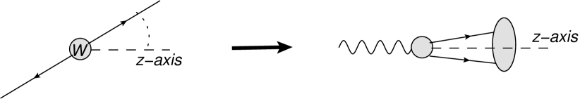
Figure 1: Sketch of two body decay of $W$ in (left) its rest frame and (right) in the lab frame.

$q$

$\theta$

boosted                  $W$

$q$

$q^{\prime}$

$q^{\prime}$

3 Jet Substructure based Polarization Study

As we already discussed that the theoretical distributions of $\cos\theta$ for longitudinally polarized $W$ and transversely polarized $W$ are proportional to $(1-|\cos\theta|^{2})$ and $(1+|\cos\theta|^{2})$ respectively. Most of the existing polarization studies of $W$ or $Z$ bosons are done with leptonic final states. However, in the case of $W$ boson, leptonic final state contains a neutrino. The weakly interacting neutrino then does not leave any trace at the detector. This makes the polarization study in leptonic decay modes little bit difficult. On the other hand, the hadronic decay modes of $W$ produce two jets at the detector. This, in principle, should make the polarization study of $W$ easier. However, effective reconstruction of jets and then $W$s makes it more difficult to study polarization of $W$ at a collider. Moreover, elimination of the huge QCD background at a collider, especially at a hadron collider, adds up to another level of difficulty. However, recent developments in the study of jets and their substructures eases some of the jobs of finding jets or subjets inside a fatjet. Although we will not report signal-background type of analysis in this article, we will try to show that the $\cos\theta_{*}$ distribution can be reproduced with a good accuracy for longitudinal and transversely polarized $W$ boson using its hadronic decay channel when $W$ is boosted and gives rise to fatjet.

If the momentum of the decaying $W$ boson is high enough, its decay products tend to be collinear. In case of hadronic decay modes, these decay products again will shower and will form collimated objects including all the collinear decay products. Now, a jet clustering algorithm may not be able to distinguish between these highly collinear decay products and will cluster these collimated final states into a single jet. These jets are popularly known as fatjets or boosted jets. These boosted jets are of high interest in the study of boosted topologies. In our study, we too considered boosted $W$ jets. Once the $W$ fatjet is found, the job remains is to find subjets inside the fatjet effectively. In this study, we have used two different methods to find the two subjets inside the boosted $W$ jets. These two methods are described in the next two subsections.

3.1 Subjet using N-subjettiness

The polarization study as described the $\cos\theta_{*}$ variable relies on the effectiveness of the construction of the subjets inside the boosted jet W. There are quite a few method by which the subjets inside a boosted jet can be found effectively. One of which is N-subjettiness Thaler:2010tr . This construction mainly relies on finding the axes of a given number of subjets. This method essentially partition the whole jet area into $n$ number of subjet area. The proper definition is as follows. Let $J$ be a boosted jet and $a_{1},a_{2},\cdots a_{n}$ are a set of $n$ axes inside the boosted jet, then we define a quantity

$$\tau_{n}=\sum_{i\in J}\min_{a_{1},a_{2},\cdots a_{n}}\left\{d_{i,1},d_{i,2},\cdots,d_{i,3}\right\}$$ (6)

where $J$ represents the full jet and $d_{i,j}$ is the distance between $i^{\text{th}}$ constituent of the jet and $j^{\text{th}}$ axis. The minimization in Eq. (6) is done over the choices of the direction of the axes.

The distance measure and axes choices are also not unique. There can be several different choices of the axes as well as the distance measure depending on the types of information one wants to extract. An exhaustive list of such choices has been given in Ref. Stewart:2015waa . For our purposes, we tried various axes choices and measures implemented in Fastjet Contrib Thaler:2010tr . We will list down the most effective choices in the result section.

3.2 Subjet using Soft Drop

Soft Drop grooming/tagging method Larkoski:2014wba was proposed to groom away the soft and wide angle constituent, which comes predominantly from PUs or UEs, inside a jet. We, too, used it as a groomer to groom away the contamination coming from PU and UE. However, we will use this to find the subjets inside the boosted jet also. To explain this, we first explain the Soft Drop algorithm below.

1. Go back to the last stage of jet clustering. Let $j_{1}$ and $j_{2}$ be the two subjets giving rise to the final jet $J$.

2. Check for the condition: $\dfrac{\min\{p_{T_{j_{1}}}\!,\ p_{T_{j_{2}}}\}}{p_{T_{j_{1}}}+p_{T_{j_{2}}}}>z_{\text{cut}}\left(\dfrac{\Delta R(j_{1},j_{2})}{R_{0}}\right)^{\beta}$

3. If the condition in 2. is satisfied, declare $J$ as the final groomed jet. Otherwise, discard the softer subjet and promote the harder one to $J$ and restart from step 1.

In this way, we get the final groomed jet. One may consider the two subjets to be the subjets of a two-pronged jet. This is good approximation since, for a two-pronged jet, the two prongs clusters first and then the two prongs combines to give rise to the final jet. As described in the algorithm itself, $z_{\text{cut}}$ and $\beta$ are parameters of Soft Drop groomer and $R_{0}$ is the radius parameter of the clustering algorithm that was chosen to cluster the jet before applying Soft Drop grooming method. One important observation is that $\beta\to\infty$ or $z_{\text{cut}}=0$ returns the original jet. Here, these two parameters are chosen suitably so that we achieve our goal. In this work, we consider this as one of the method to find subjets of the boosted jets we will be considering later. Here again, we checked with a number of different choices of these two parameters. The best choices for our purposes will be given in the result section.

As we already mentioned that the two variables $p_{\theta}$ and $z_{j}$ has already been suggested in the literature de2020measuring ; roloff2021sensitivity . Our main objective of this report is to improve on the analysis. As we already explained that $p_{\theta}$ correctly reproduces $\cos\theta_{*}$, where $\theta_{*}$ is the angle between the two decay products of $W$ in its rest frame. In the limit where $\theta_{*}$ is $\pi/2$, both the decay products make almost same angle with respect to the boost axis of the decaying $W$ and after the boost, in the lab frame, they share almost equal energy inside the fatjet. However, if $\theta_{*}\to 0$ or $\pi$, one decay product is parallel to the boost axis while the other is anti-parallel to the boost axis. Hence, after the boost the parallel one becomes highly energetic and the anti-parallel one becomes soft and wide angle. Because of this, finding the subjet effectively is difficult in the case of $|\cos\theta_{*}|\to 1$. In our study, we mainly focused on this region so the discrimination between longitudinal and transverse $W$ bosons can be improved. We applied the above two methods to improve upon the earlier studies available in the literature.

4 Generation of Templates

As discussed earlier, we are interested in reconstructing boosted $W$ jet and want to separate the two differently polarized boosted $W$ boson using the variables $p_{\theta}$ and $z_{j}$. In this regard, we need to calibrate two kinds of samples, one, which can contain a fully longitudinally polarized boosted $W$ bosons and another with fully transversely polarized boosted $W$ bosons. For this purpose, we used two specific interaction Lagrangians which can be implemented in FeynRules Alloul_2014 and already used in Ref. de2020measuring .

4.1 Template model

Longitudinally polarized $W$ bosons can be generated via a fictitious scalar particle $\phi_{s}$ which have a Higgs-like couplings to W bosons and gluons,

$$\mathcal{L}_{s}=c_{s}^{w}\phi_{s}W^{\mu}W_{\mu}+c_{s}^{g}\phi_{s}G^{\mu\nu}G_{\mu\nu}$$ (7)

$c_{s}^{w}$ and $c_{s}^{g}$ are the coupling constants. We can see that the interaction of the scalar with $W$ bosons is through a non-gauge invariant, renormalizable term and it picks out longitudinal $W$ bosons at high energies as per Goldstone equivalence theorem. That is why there will be a small admixture of transverse $W$ bosons if we produce $W$ via the s-channel process through $\phi_{s}$. However, the fraction of transverse $W$ they will be suppressed by a fraction $\sim\!\frac{m^{4}_{W}}{E^{4}}\simeq 10^{-3}-10^{-4}$ for W bosons with energies of order $500$ GeV to $800$ GeV.

On the other hand, transversely polarized $W$ bosons can be produced by using non-renormalizable dimension-5 interaction terms for a fictitious pseudo-scalar field $\phi_{ps}$. It can couple to $W$s and gluons via the terms like

$$\mathcal{L}_{ps}=d_{s}^{w}\phi_{ps}W^{\mu\nu}\tilde{W}_{\mu\nu}+d_{s}^{g}\phi_{ps}G^{\mu\nu}\tilde{G}_{\mu\nu}$$ (8)

For the sample of longitudinal $W$, we produced events in MadGraph5 Alwall:2014hca at a centre-of-mass energy $\sqrt{s}$ = 14 TeV via the process $pp\rightarrow\phi_{s}$ with $\phi_{s}\rightarrow W^{+}W^{-}$ and for the sample for purely transverse $W$, the same type of $s$-channel process considered with $\phi_{s}$ replaced by $\phi_{ps}$. Since we will be studying the polarization of one of the boosted $W$ jet, one $W$ boson was allowed to decay hadronically and the other was forced to decay leptonically during the event generation using MadGraph5.

From Eq. (8), it can be shown that the amplitude for $W$ boson production from the pseudo-scalar vertex have the form $\mathcal{M}\propto\epsilon_{\mu\nu\rho\sigma}p_{1}^{\mu}\epsilon_{1}^{\nu}p_{2}^{\rho}\epsilon_{2}^{\sigma}$, where $\epsilon_{\mu\nu\rho\sigma}$ is the fully-antisymmetric tensor and $p_{i}$, $\epsilon_{i}$ represent the four-momentum and polarization vector for the $i^{\text{th}}$ $W$. This form in the amplitude helps us to get a purely transverse polarization vectors. As we are interested in boosted $W$ region produced via heavy resonance decay, the mass of the scalar/pseudo-scalar are chosen $\sim$1 TeV.

4.2 Generation of Sample Events

The following procedures have been conducted to generate the sample events for our analysis.

1. For both (longitudinal and transverse) the cases, we generated 8 lakh events in each of the cases, with an intermediate scalar and pseudo-scalar using MadGraph5 Alwall:2014hca . At the parton level event generation, we demand that the $W$ bosons have $p_{T}>300.0$ GeV for both the cases. In order to get relatively pure longitudinal sample, the events with production of $W$ boson via $\phi_{s}$ has a cut on momentum of $W$ boson which is $>500.0$ GeV. At this parton level, we can construct the variables by using relations,

   $$|\cos\theta_{*}|=\frac{|\Delta E|}{p_{W}}$$ (9)

   $$z_{j_{*}}=\frac{p_{T}^{leading}}{p_{T}^{W}}$$ (10)

   Here $p_{T}^{leading}$ is the $p_{T}$ of our leading hadron, $p_{T}^{W}$ is the $p_{T}$ of $W$ boson and $|\Delta E|$ is the absolute value of the energy difference of two hadrons generated from $W$ decay.

2. We then used Pythia8 Sjostrand:2014zea ; Sjostrand:2006za to shower and hadronize these parton level events generated by MadGraph5. For the analysis after showering and hadronization, we used the parton level events without any cut and with underlying events turned on.

3. We then cluster the final state hadrons with $|\eta|<$ 4.0 using the Cambridge-Aachen algorithm in FastJet Cacciari:2011ma ; Cacciari:2005hq with a jet radius $R_{0}$ = 1.0 and use two different methods to reconstruct two prongs from the fatjet as described in the previous section. As we can see that the pure longitudinal and transverse samples have differences in the distributions in the plane of the two variables, $p_{\theta}$ and $z_{j}$. Since we are expecting two subjets in a $W$ fatjet, we have taken $n=2$ for the calculation of N-subjettiness variable $\tau_{n}$ as defined in Eq. (6) for all the cases. The different choice of axes and distance measures in N-subjettiness technique and different $z_{cut}$ and $\beta$ cut in Soft Drop technique can be useful depending on which type of polarization we wants to study. This will be explained in details in the next section where best case scenarios will be studies with different kind of setups.

   • In the case where we are interested in reconstructing longitudinal $W$, for N-subjettiness, we used ‘OnePass General $E_{T}$ General $K_{T}$ Axes’ choice with jet radius $R_{0}$ = 0.2 and $p$ = 0.6 (the limiting cases are $k_{t}$ and Cambridge-Aachen axes choices for $p=1$ and $p=0$ respectively) Catani:1991hj ; Catani:1993hr . With this, we used ‘Unnormalized Measure’ with $\beta$ = 1.0 Stewart:2015waa .

   • When we consider transverse $W$ as our best case, for N-subjettiness we used same axis and measure choice with a different $p$ value, $p$ = 0.05.

   • For longitudinal $W$ best case two Soft Drop parameters are chosen as $z_{\text{cut}}=0.26$ and $\beta=1.0$ while for transverse $W$ analysis they are set at $z_{\text{cut}}=0.09$ and $\beta$ = 2.1.

   For all the cases the events are selected if the reconstructed $W$ (fatjet) has a $p_{T}>$ 300.0 GeV

4. Detector level simulation are done by using Delphes de_Favereau_2014 . We then added pile-up events by considering minbias pile-up. After that the samples are reconstructed with the similar way as described in the last point with the same choices of N-subjettiness and Soft Drop parameters.

5. For all the cases the final samples are chosen with the following tagging cuts on the $W$ jets,
   $\bullet$ Mass cut: 60 GeV $<M_{W/J}<$ 100 GeV, where $M_{J}$ is the mass of the fatjet.

We will be carrying out the analysis at three different levels, viz. (a) parton level, (b) pythia level, and (c) delphes level. Parton level means the variables were calculated at the parton level final state i.e. after event generation in MadGraph5 while pythia level means the variables were calculated after showering and hadronization by Pythia8. The variables calculated after detector effects using Delphes are represented by delphes level. At the parton level analysis, we expect to get the similar distribution as Eq. (3) by constructing the variable $\cos\theta_{*}$ and $z_{j_{*}}$ at the lowest order in QCD process using Eq. (4) and Eq. (5). In pythia level calculations, the quarks from $W$ boson decay undergo through showering and hadronization process to give rise to hadrons as final state particles. These final state hadrons are then clustered as jets. For detector level simulation pile up effects are also added with those and the jets are formed after the detector simulation. As we are interested in boosted $W$ region, the jets coming from $W$ decay are highly collimated and most often ends up by providing a fatjet. To classify the fatjets correspond to $W$ bosons we can use the mass cut described before. Along with that, to reconstruct the variables, we need to find out the subjets from the fatjet by using jet substructure techniques. As discussed earlier that we used N-subjettiness and Soft Drop for this purpose. After finding out the two prongs from the fatjet we reconstruct the two variables $p_{\theta}$ and $z_{j}$ as

$$p_{\theta}=\frac{|\Delta E^{reco}|}{p_{W}^{reco}}$$ (11)

$$z_{j}=\frac{p_{T}^{leading,reco}}{p_{T}^{W,reco}}$$ (12)

where the superscript ‘reco’ has been added to represent the reconstructed values for the momenta and the energies. So ${p_{W}^{reco}}$ represents the magnitude of the momentum of reconstructed $W$ which is nothing but the magnitude of momentum of the fatjet ($|p_{J}|$) at the hadron level or at the detector level reconstruction of the $W$ momentum. $|\Delta E^{reco}|$ can be calculated by taking the difference in the energies of the two subjets reconstructed at pythia and delphes level. Similarly, $p_{T}^{leading,reco}$ is the $p_{T}$ of leading subjet inside boosted $W$ jet and $p_{T}^{W,reco}$ is the transverse momentum of reconstructed $W$.

5 Result

5.1 Best case scenarios

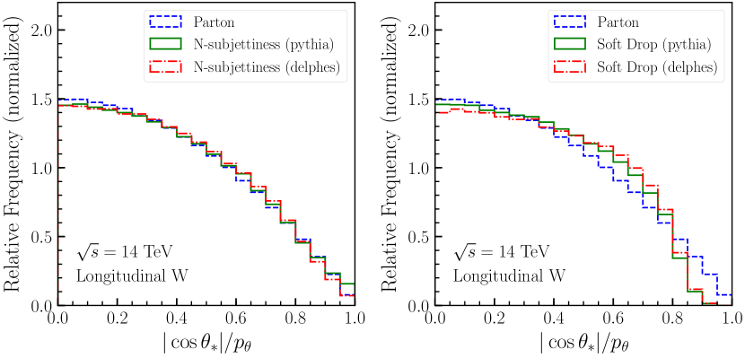
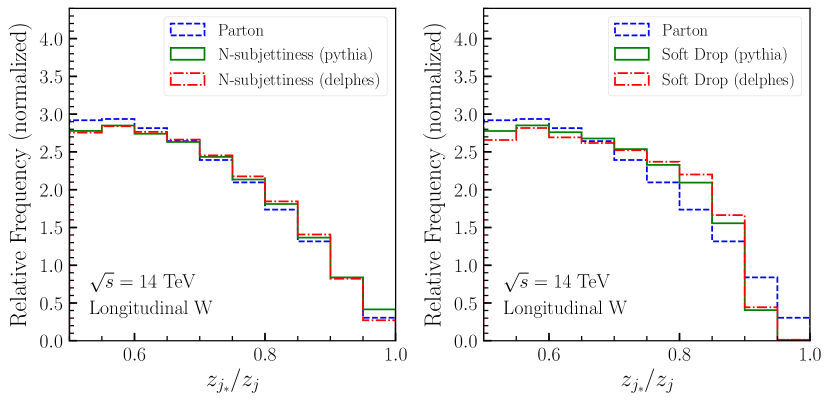
Figure 2: Normalized distribution of angular variable $p_{\theta}$ (upper panel) and momentum balance $z_{j}$ (lower panel) for longitudinally polarized $W$. The distributions are shown for parton level (blue dashed), pythia level (green solid) and delphes level (red dash dotted) analysis with N-subjettiness (left panel) and Soft drop (right panel) techniques to find the subjets.

As we mentioned earlier that the study of polarization of $W$ boson depends on how accurately the two subjets inside these boosted jets can be reconstructed. In order to get close enough distribution of $p_{\theta}$ to $|\cos\theta|$, we have varied different parameters of Soft Drop and N-subjettiness. We first did a thorough scan over these parameters to get a good match to the theoretical distribution of $|\cos\theta|$. We did not carry out the matching for $z_{j}$ variable with $z_{j_{*}}$ since these two variables are highly correlated. In our study, we found that we need to take different values of the parameters for longitudinal case than the transverse case. We show these matching in Figure 2 for longitudinally polarized $W$ (the Lagrangian is described by Eq. (7)). As mentioned earlier that we carried out the analysis at three different levels, viz. (a) parton level, (b) pythia level, and (c) delphes level. In all the panels of Figure 2, blue dashed, green solid and red dash dotted histograms represent the distributions of variables for parton level, pythia level and delphes level analysis respectively. We can see that both N-subjettiness analysis and Soft Drop analysis provides good matching for the longitudinal case for both the variables $p_{\theta}$ and $z_{j}$. The distribution is little off near the value 1. The reason for this is that one of the subjet is very soft in that region and hence it is difficult to reconstruct that soft subjet effectively in that region.

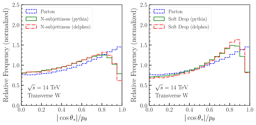
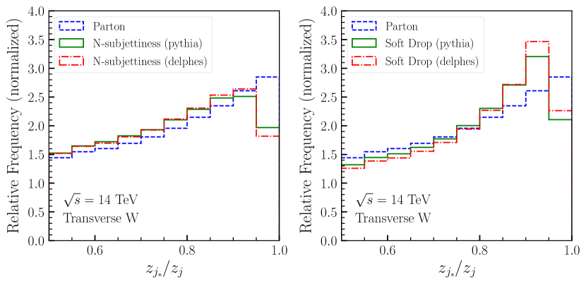
Figure 3: Normalized distribution of angular variable $p_{\theta}$ (upper panel) and momentum balance $z_{j}$ (lower panel) for transversely polarized $W$. The convention for the colours and the level are similar to Figure 2.

The same analysis has been done for the transverse case also. Figure 3 shows the distributions of the same variables for the parton, pythia and delphes level analyses. The conventions (colour, label etc.) are similar to that of Figure 2. We see the same feature here again i.e. the distribution is not very accurate near 1 because one of the subjet is very soft here.

As we mentioned that the parameter choices for best case scenarios are different for the longitudinal case than the transverse one. We tabulate the parameter choices for best case scenarios for both the longitudinal and transverse cases in Table 1. The reason for the different choices are quite clear from the distribution of $p_{\theta}$ as well as $z_{j}$ as shown in Figure 2 and Figure 3. The distributions peak near 0 for the case of longitudinal $W$ whereas they peak near 1 for the case of transverse $W$. For the case of Soft Drop as a method of finding the subjets inside boosted $W$, we need very soft $z_{\text{cut}}$ in order to keep the softer subjet of the final jet. As in the case of transverse $W$, we need to the peak near 1, the $z_{\text{cut}}$ value should be smaller than that of longitudinal $W$. However, $\beta$ parameter of is mostly independent of which type of polarization is being dealt with.

N-subjettiness
	Axes choice	Measure choice	$\beta$-value	$p$-value
Longitudinal  $W$ Best case scenario	‘OnePass General $E_{T}$  General  $k_{T}$ Axes’	Unnormalized Measure	1.0	0.6
Transverse  $W$   Best case scenario	‘OnePass General $E_{T}$  General  $k_{T}$ Axes’	Unnormalized  Measure	1.0	0.05

Soft Drop
	$\beta$-value	$z_{\text{cut}}$-value
Longitudinal  $W$ Best case scenario	1.0	0.26
Transverse  $W$   Best case scenario	2.1	0.09

Table 1: Parameter choices for the two techniques used to find subjets inside $W$ fatjet. These values of parameters are taken to optimize the templates for longitudinally and transversely polarized $W$.

5.2 Separability

We then tried to check the separability between the longitudinal and transverse $W$ bosons study. We did this in terms of Receiver Operating Characteristic (ROC) curves. When there is difference in the distribution of a variable coming from two different types of sources, we may try to get a score of their separability via ROC curves. These curves are usually drawn to show how much a particular distribution can be rejected at what acceptance level of the other. This is usually done for signal and background analysis where our main aim is to accept signal and reject background effectively. However, ROC can also give us a sense of separability of two distribution. Although longitudinal and transverse distributions are not signal and background analysis, we have drawn their ROC curves to show their separability via this method. If two distributions are identical, the area under the ROC curves are 0.5. In case there are separation between the two different distribution, the area under the curve varies from 0.5 to 1 with 1 being the completely separable. Hence, closer the value of area under the ROC curve to 1, better they can be separated.

We consider both cases where, in one we want to get longitudinally polarized $W$ event over the transverse one (see Figure 4) and here we use the parameter choice for the Longitudinal $W$ best case scenario from Table 1. In another case we try to get the transversely polarized $W$ dominated region over the longitudinal one (see Figure 5) and here we use the JSS parameters as per the transverse $W$ best case scenario from Table 1 using two feature variables, $p_{\theta}$ and $z_{j}$. To get better separability, we explore some recently developed techniques like Gradient Boosted Decision Trees Chen_2016 . The toolkit used for Gradient boosting is XGBoost Chen_2016 . For gradient boosted Decision Tree method of separation, we consider $\sim$5500 estimators and maximum depth of 4 where the learning rate varies depending on the achievement to separate longitudinal and transverse polarized samples at different level of measurements (generator level, pythia level or detector level) without overtraining. For parton level analysis in both the cases our learning rate is 0.03 and we have used 80% of our total dataset for training purpose and 20% for validation, where for other kind of analysis our learning rate is 0.001 and we used 70% of the data to train our sample and 30% for validation.

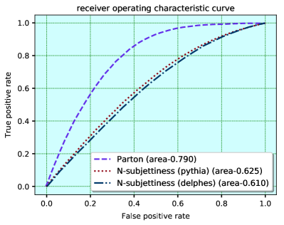
Figure 4: ROC curves to illustrate the separability between two templates, viz. longitudinal and transverse. The parameter choices are taken to optimize the longitudinal template.

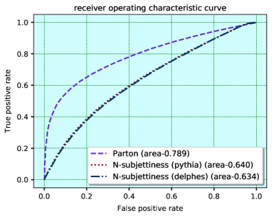
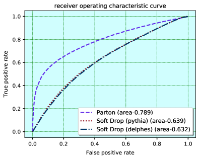
Figure 5: ROC curves to illustrate the separability between two templates, viz. longitudinal and transverse. The parameter choices are taken to optimize the transverse template.

In Figure 4 we can see the ROC curve where our signal is coming from longitudinally polarized $W$ decay and our background is coming from transversely polarized $W$ decay. In left side plot we represent parton level analysis and also pythia level and detector level analysis with N-subjettiness technique. On the other hand in right side plot similar things are represented by measuring with Soft Drop technique. Alternatively Figure 5 shows the ROC curve where the signal is characterized by the events with transversely polarized $W$ and the background events are coming from longitudinally polarized $W$ decay. Here also left and right side plot portrays the separability using N-subjettiness and Soft Drop techniques respectively. For all the cases, area under the ROC curve are listed in Table 2.

Measurement of separability (Area under the ROC curve)
Analysis level/techniques	Longitudinal  $W$ Best case scenario	Transverse  $W$ Best case scenario
Parton	0.790	0.789
N-subjettiness (pythia)	0.625	0.640
N-subjettiness (delphes)	0.610	0.634
Soft Drop (pythia)	0.588	0.639
Soft Drop (delphes)	0.589	0.632

Table 2: Area under the ROC curves for different level of analysis

From Table 2, we can see that at parton level we can achieve better separability among all the cases. For Longitudinal best case scenario, at pythia level both N-subjettiness and Soft Drop achieve similar kind of separability where at delphes level, Soft Drop perform batter than N-subjettiness. On the other hand, for transverse best case scenario, all the techniques doing batter than previous case and at detector level analysis N-subjettiness doing batter than Soft Drop.

One of the possible shortcomings of these technique is over-training of the data sample where the training sample gives extremely good accuracy but the test sample fails to achieve that and we can see a noticeable difference in the ROC curve of training and testing case. We have explicitly checked that with our choice of parameters the algorithm we used does not overtrain.

5.3 Template fitting

We now use the above templates of longitudinal and transverse $W$ bosons to acquire information from a mixed sample. For this study, we first prepared sample events, which has admixture of longitudinal and transverse $W$ bosons in it. We then try to fit the this mixed sample events with the templates we generated earlier. Let $L(x)$ and $T(x)$ be the distribution for the variable $x$ for the two templates of longitudinally and transversely polarized $W$ bosons, respectively. These distributions are after the detector simulation and hence are not necessarily the same as the theoretical distribution. Let a mixed sample has the distribution $M(x)$ for the same variable $x$. The fraction, $\alpha$, of longitudinally polarized $W$ boson in the the mixed sample may be estimated by minimizing the following quantity.

$$\chi^{2}=\sum_{i\,\in\,\text{bins}}\left|M(x_{i})-\alpha L(x_{i})-(1-\alpha)T(x_{i})\right|^{2}$$ (13)

The minimization over the fraction $\alpha$ gives the estimate for $\alpha$ as

$$\alpha=\frac{\sum_{i\,\in\,\text{bins}}\left(M(x_{i})-T(x_{i})\right)\left(L(x_{i})-T(x_{i})\right)}{\sum_{i\,\in\,\text{bins}}\left(L(x_{i})-T(x_{i})\right)^{2}}$$ (14)

In this part of the study, we used the Delphes level distributions as our templates for longitudinally and transversely polarized $W$. We then prepared mixed sample events with three different fraction of 25%, 50% and 75%. We then tried to estimate the value of $\alpha$ for these mixed sample cases. The estimated values are presented in Table 3.

Subjet found	Template optimized	Sample prepared	Estimated $\alpha$
using	best for	with $\alpha$
N-subjettiness	Longitudinal	0.25	0.169
		0.50	0.454
		0.75	0.731
	Transverse	0.25	0.239
		0.50	0.499
		0.75	0.746
Soft Drop	Longitudinal	0.25	0.182
		0.50	0.480
		0.75	0.734
	Transverse	0.25	0.224
		0.50	0.471
		0.75	0.703

Table 3: Estimated fraction (4th column) and actual fraction (3rd column) of longitudinally polarized $W$ in a mixed sample in the two technique to find the subjets.

We have done this analysis with both the subjet finding methods, viz. N-subjettiness as well as Soft Drop method, and for both the scenarios with the templates being optimized best for longitudinally and transversely polarized $W$. In this part of the analysis, we used only $p_{\theta}$ variable. We can see from Table 3 that the fraction $\alpha$ can be estimated with relatively good accuracy for the case when template is best optimized for transversely polarized $W$ in the N-subjettiness subjet finding method.

6 Summary and Outlook

To summarize, we have studied the polarization states of hadronically decaying boosted $W$ boson. We have considered 14 TeV centre-of-mass energy at the LHC in this study. We first generated approximately pure longitudinal and transverse $W$ boson by taking appropriate template models and high enough $p_{T}$ cut to keep hadronic $W$ as a fatjet. The analysis was done using angular variable $p_{\theta}$ (a proxy for $|\cos\theta|$) and momentum balance $z_{j}$ calculated using momenta and energies of the two subjets inside boosted $W$s. We employed the technique of N-subjettiness and Soft Drop to find the two subjets inside $W$ fatjets. The analysis was done at three different levels viz. (a) parton level, (b) pythia level, and (c) detector level. The different parameters of N-subjettiness and Soft Drop were optimized to achieve better match to the parton level distribution of these two variables for longitudinally and transversely polarized $W$ bosons separately. Although the optimized values of the parameters are different in two differently polarized cases, the separability is quite good in these two cases. We then used the templates to get an estimate of the fraction of longitudinally polarized $W$ in a set of mixed sample events. The estimate are better for the case when the template is optimized for transversely polarized $W$ than the longitudinal case.

The primary improvement of this study is to find the subjets inside a fatjet with a relatively better accuracy. This techniques can be used in the studies where the subjets inside a boosted jet is needed to be found. Although we did not carry out signal-background analysis in this study, this technique can be used to do such type of studies. This improvement may be achieved other boosted objects like $Z$, $H$, $t$, or other heavy BSM particles.

References

- (1) S. P. MARTIN, A supersymmetry primer, Advanced Series on Directions in High Energy Physics (Jul, 1998) 1–98.
- (2) C. Csáki, S. Lombardo, and O. Telem, Tasi lectures on non-supersymmetric bsm models, 2018.
- (3) W. Kilian, M. Sekulla, T. Ohl, and J. Reuter, High-energy vector boson scattering after the higgs boson discovery, Physical Review D 91 (May, 2015).
- (4) W. Kilian, T. Ohl, J. Reuter, and M. Sekulla, Resonances at the lhc beyond the higgs boson: The scalar/tensor case, Physical Review D 93 (Feb, 2016).
- (5) T. Han, D. Krohn, L.-T. Wang, and W. Zhu, New physics signals in longitudinal gauge boson scattering at the lhc, Journal of High Energy Physics 2010 (Mar, 2010).
- (6) J. Brehmer, Polarised WW Scattering at the LHC, Master’s thesis, U. Heidelberg, ITP, 2014.
- (7) S. Chatrchyan, V. Khachatryan, A. M. Sirunyan, A. Tumasyan, W. Adam, T. Bergauer, M. Dragicevic, J. Erö, C. Fabjan, M. Friedl, and et al., Measurement of the polarization ofwbosons with large transverse momenta inw+jetsevents at the lhc, Physical Review Letters 107 (Jul, 2011).
- (8) G. Aad, B. Abbott, J. Abdallah, S. Abdel Khalek, A. A. Abdelalim, O. Abdinov, B. Abi, M. Abolins, O. S. AbouZeid, and et al., Measurement of the w boson polarization in top quark decays with the atlas detector, Journal of High Energy Physics 2012 (Jun, 2012).
- (9) S. De, V. Rentala, and W. Shepherd, Measuring the polarization of boosted, hadronic bosons with jet substructure observables, 2020.
- (10) J. M. Butterworth, A. R. Davison, M. Rubin, and G. P. Salam, Jet substructure as a new Higgs search channel at the LHC, Phys. Rev. Lett. 100 (2008) 242001, [arXiv:0802.2470].
- (11) J. Thaler and K. Van Tilburg, Identifying boosted objects with n-subjettiness, Journal of High Energy Physics 2011 (Mar, 2011).
- (12) A. J. Larkoski, S. Marzani, G. Soyez, and J. Thaler, Soft Drop, JHEP 05 (2014) 146, [arXiv:1402.2657].
- (13) M. R. Buckley, H. Murayama, W. Klemm, and V. Rentala, Discriminating spin through quantum interference, Physical Review D 78 (Jul, 2008).
- (14) M. R. Buckley, B. Heinemann, W. Klemm, and H. Murayama, Quantum interference effects among helicities at cern lep-ii and fermilab tevatron, Physical Review D 77 (Jun, 2008).
- (15) A. Ballestrero, E. Maina, and G. Pelliccioli, W boson polarization in vector boson scattering at the lhc, Journal of High Energy Physics 2018 (Mar, 2018).
- (16) E. Mirkes and J. Ohnemus, Wandzpolarization effects in hadronic collisions, Physical Review D 50 (Nov, 1994) 5692–5703.
- (17) W. J. Stirling and E. Vryonidou, Electroweak gauge boson polarisation at the lhc, Journal of High Energy Physics 2012 (Jul, 2012).
- (18) A. Belyaev and D. Ross, What does the cms measurement of w-polarization tell us about the underlying theory of the coupling of w-bosons to matter?, Journal of High Energy Physics 2013 (Aug, 2013).
- (19) J. Roloff, V. Cavaliere, M.-A. Pleier, and L. Xu, Sensitivity to longitudinal vector boson scattering in semi-leptonic final states at the hl-lhc, 2021.
- (20) J. Thaler and K. Van Tilburg, Identifying Boosted Objects with N-subjettiness, JHEP 03 (2011) 015, [arXiv:1011.2268].
- (21) I. W. Stewart, F. J. Tackmann, J. Thaler, C. K. Vermilion, and T. F. Wilkason, XCone: N-jettiness as an Exclusive Cone Jet Algorithm, JHEP 11 (2015) 072, [arXiv:1508.01516].
- (22) A. Alloul, N. D. Christensen, C. Degrande, C. Duhr, and B. Fuks, Feynrules 2.0 — a complete toolbox for tree-level phenomenology, Computer Physics Communications 185 (Aug, 2014) 2250–2300.
- (23) J. Alwall, R. Frederix, S. Frixione, V. Hirschi, F. Maltoni, O. Mattelaer, H. S. Shao, T. Stelzer, P. Torrielli, and M. Zaro, The automated computation of tree-level and next-to-leading order differential cross sections, and their matching to parton shower simulations, JHEP 07 (2014) 079, [arXiv:1405.0301].
- (24) T. Sjöstrand, S. Ask, J. R. Christiansen, R. Corke, N. Desai, P. Ilten, S. Mrenna, S. Prestel, C. O. Rasmussen, and P. Z. Skands, An introduction to PYTHIA 8.2, Comput. Phys. Commun. 191 (2015) 159–177, [arXiv:1410.3012].
- (25) T. Sjostrand, S. Mrenna, and P. Z. Skands, PYTHIA 6.4 Physics and Manual, JHEP 05 (2006) 026, [hep-ph/0603175].
- (26) M. Cacciari, G. P. Salam, and G. Soyez, FastJet User Manual, Eur. Phys. J. C 72 (2012) 1896, [arXiv:1111.6097].
- (27) M. Cacciari and G. P. Salam, Dispelling the myth for the jet-finder, Phys. Lett. B 641 (2006) 57–61, [hep-ph/0512210].
- (28) S. Catani, Y. L. Dokshitzer, M. Olsson, G. Turnock, and B. R. Webber, New clustering algorithm for multi - jet cross-sections in e+ e- annihilation, Phys. Lett. B 269 (1991) 432–438.
- (29) S. Catani, Y. L. Dokshitzer, M. H. Seymour, and B. R. Webber, Longitudinally invariant clustering algorithms for hadron hadron collisions, Nucl. Phys. B 406 (1993) 187–224.
- (30) J. de Favereau, C. Delaere, P. Demin, A. Giammanco, V. Lemaître, A. Mertens, and M. Selvaggi, Delphes 3: a modular framework for fast simulation of a generic collider experiment, Journal of High Energy Physics 2014 (Feb, 2014).
- (31) T. Chen and C. Guestrin, Xgboost, Proceedings of the 22nd ACM SIGKDD International Conference on Knowledge Discovery and Data Mining (Aug, 2016).