Extensions of Karger’s Algorithm: Why They Fail in Theory and How They Are Useful in Practice

Abstract

The minimum graph cut and minimum $s$-$t$-cut problems are important primitives in the modeling of combinatorial problems in computer science, including in computer vision and machine learning. Some of the most efficient algorithms for finding global minimum cuts are randomized algorithms based on Karger’s groundbreaking contraction algorithm. Here, we study whether Karger’s algorithm can be successfully generalized to other cut problems. We first prove that a wide class of natural generalizations of Karger’s algorithm cannot efficiently solve the $s$-$t$-mincut or the normalized cut problem to optimality. However, we then present a simple new algorithm for seeded segmentation / graph-based semi-supervised learning that is closely based on Karger’s original algorithm, showing that for these problems, extensions of Karger’s algorithm can be useful. The new algorithm has linear asymptotic runtime and yields a potential that can be interpreted as the posterior probability of a sample belonging to a given seed / class. We clarify its relation to the random walker algorithm / harmonic energy minimization in terms of distributions over spanning forests. On classical problems from seeded image segmentation and graph-based semi-supervised learning on image data, the method performs at least as well as the random walker / harmonic energy minimization / Gaussian processes.

(2cm,26.5cm) © 2021 IEEE. Personal use of this material is permitted. Permission from IEEE must be obtained for all other uses, in any current or future media, including reprinting/republishing this material for advertising or promotional purposes, creating new collective works, for resale or redistribution to servers or lists, or reuse of any copyrighted component of this work in other works.

1 Introduction

Minimum graph cuts have been applied to machine learning problems for a long time. They have been used in natural language processing [33] and especially in computer vision, for example in segmentation [40, 34, 2], restoration [13], and energy minimization more generally [21]. Nowadays, they still form an important part of many deep learning pipelines, for example for segmentation [42, 28, 29, 25, 26], image classification [31], and recently also neural style transfer [43].

For finding global minimum cuts (defined together with all other terminology in Section 2), Karger’s contraction algorithm [16, 19] started a wave of randomized algorithms solving this problem efficiently [17, 8, 10, 27].

Thanks to these randomized algorithms, global mincuts can, somewhat surprisingly, be found more efficiently than $s$-$t$-mincuts. An interesting question is therefore to what extent randomized algorithms can be applied to other graph cut problems, and in particular whether Karger’s algorithm can be fruitfully extended. An especially important cut problem are $s$-$t$-mincuts. While approximating them is possible in nearly linear time in the number of edges [20, 35] and has also been studied using randomized algorithms based on graph sparsification [1], it is to our knowledge still an open question whether Karger’s algorithm can be modified to efficiently find $s$-$t$-mincuts.

In Section 3, we give a definitive answer to this question by proving that a large class of extensions of Karger’s contraction algorithm can in general not exactly solve the $s$-$t$-mincut problem efficiently. Our result also applies to the normalized cut problem [36], which, like the $s$-$t$-mincut, plays an important role in image segmentation.

However, extensions of Karger’s algorithm can still be useful if applied in the right way. In Section 4, we show how a straightforward extension of Karger’s algorithm can be used successfully for seeded segmentation / semi-supervised learning tasks. We interpret this extension as a forest sampling method and observe its similarities to the random walker algorithm [11] for seeded graph segmentation. In semi-supervised learning, the same algorithm is known as harmonic energy minimization [44] or Gaussian Processes, so the same observations apply.

The main contribution of this paper is purely conceptual. Still, in Section 5 we show in two classical experiments that the proposed algorithm compares well against the random walker / harmonic energy minimization, perhaps the most influential algorithm in seeded segmentation / semi-supervised learning to date. Since our method has an asymptotic time complexity of only $\mathcal{O}(m)$ on a graph with $m$ edges, it can be seen as an efficient alternative to the random walker algorithm / harmonic energy minimization, while also giving a probabilistic output.

Related work

The most closely related work is the typical cut algorithm [9], which uses an ensemble of cuts generated by Karger’s algorithm for clustering without seeds. In contrast, the method described here uses cuts generated by a slight variation of Karger’s algorithm to solve seeded segmentation problems. In this setting, there is a very natural way to get a segmentation from the ensemble of cuts, as well as a natural stopping point for the contraction, which for the typical cut is a free parameter.

2 Background

All graphs considered in this paper are undirected and connected and have non-negative edge weights. We write such a graph as a tuple $G=(V,E,w)$ of a set of vertices $V$, an edge set $E$ and a weight function $w:E\to\mathbb{R}_{\geq 0}$. We denote the number of vertices by $n:=\left\lvert V\right\rvert$ and the number of edges by $m:=\left\lvert E\right\rvert$. We also write $w_{e}$ for the weight $w(e)$ of an edge $e\in E$ and $w_{uv}$ for the weight of the edge between vertices $u,v\in V$. If no edge is present, $w_{uv}$ is defined as zero. $w(A,B):=\sum_{a\in A,b\in B}w_{ab}$ is the sum of edge weights connecting two subsets $A,B\subset V$.

A graph cut is a partition of the vertices $V$ of a graph into two disjoint non-empty subsets $A$ and $B$ such that $V=A\cup B$. The cut set of such a cut is the set of all edges with one endpoint in $A$ and one in $B$. The sum $w(A,B)$ of the weights of all edges in the cut set is called the weight or cost of the graph cut.

We will describe three different cut problems here: the global minimum cut, the $s$-$t$-minimum cut and the normalized cut.

A (global) minimum cut

of a graph – or mincut for short – is a cut with minimal cost. In other words, the minimum cut problem is given by

$$\operatorname*{arg\,min\>}_{\text{partitions }(A,B)\text{ of }V}w(A,B)\,.$$ (1)

An $s$-$t$-cut

of a graph $G$ is a graph cut that separates two given vertices $s\neq t\in V$. In the $s$-$t$-mincut problem, the goal is to find an $s$-$t$-cut with minimal cost, i.e.

$$\operatorname*{arg\,min\>}_{\text{partitions }(S,T)}w(S,T)\quad\text{such that }s\in S,t\in T\,.$$ (2)

For convenience, we define an $s$-$t$-graph as a tuple $(G,s,t)$ of a graph and two vertices $s\neq t\in V.$

We also mention here the notion of $\alpha$-minimal cuts. A global cut $(A,B)$ is $\alpha$-minimal if its cost is within a factor $\alpha$ of the global minimum cut,

$$w(A,B)\leq\alpha\min_{\begin{subarray}{c}\text{partitions }\\ (A^{\prime},B^{\prime})\end{subarray}}w(A^{\prime},B^{\prime})\,,$$ (3)

where $\alpha$ is some positive real number $>1$. The same concept can of course be applied to define an $\alpha$-minimal $s$-$t$-cut as an $s$-$t$-cut that has a cost within a factor $\alpha$ of the $s$-$t$-mincut.

The normalized cut

[36] generates more balanced cuts than the minimum cut objective, which makes it particularly well suited for image segmentation. It minimizes

$$\operatorname{ncut}(A,B):=\frac{w(A,B)}{w(A,V)}+\frac{w(A,B)}{w(B,V)}$$ (4)

over the partitions $(A,B)$ of the graph. Note that since $w(A,V)\overset{\text{(def)}}{=}\sum_{a\in A,v\in V}w_{av}$, this term counts the internal weights of $A$ twice. Solving the normalized cut problem exactly is NP-complete, but the solution can be approximated with a spectral method [36].

2.1 Karger’s contraction algorithm

Karger’s algorithm is a Monte Carlo algorithm for finding global minimum graph cuts, meaning that it has a fixed runtime but is not guaranteed to find the best cut. It is based on contractions of edges in a graph. Given a graph $G=(V,E,w)$ and two vertices $v_{1},v_{2}\in V$, the contracted graph $G/\{v_{1},v_{2}\}$ is obtained as follows:

1. $v_{1}$ and $v_{2}$ with all their edges are removed and a new vertex $u$ is added.

2. For each edge $\{v_{i},x\}\in E$ with $x\notin\{v_{1},v_{2}\}$, a new edge $\{u,x\}$ with the same weight is added, for $i=1,2$.

3. If $u$ now has several edges to the same vertex, they are merged into one by adding their weights.

Karger’s algorithm simply repeatedly chooses an edge at random and contracts it until only two vertices remain. The remaining edges then define a cut set. Each edge is chosen for contraction with probability proportional to its weight. The precise algorithm is described in algorithm 1.

Input : graph $G$

Output : contracted graph with 2 vertices

while $G$ has more than 2 vertices do

       choose an edge $\{u,v\}$ with probability proportional to its weight;

       $G\leftarrow G/\{u,v\}$;

      

return $G$;

Algorithm 1 Karger’s contraction algorithm

Of course, this algorithm does not always produce a minimum cut. To increase the success probability, the algorithm is run several times and the best cut is returned. This can be sped up by sharing computations between runs [18, 19] but doing so does not affect any of the arguments in this paper, so we will ignore it.

The reason why Karger’s algorithm is useful for finding minimum cuts is the following theorem, which says that – compared to the success probability of $2^{-n+1}$ that uniform sampling of cuts would give – Karger’s algorithm finds a minimum cut with relatively high probability on a single run. This means that a polynomial number of runs is enough to find a minimum cut with high probability.

Theorem 1 ([16]).

The probability of finding any given mincut with Karger’s algorithm is at least ${n\choose 2}^{-1}$.

The key idea of the proof is that the cost of a global minimum cut is only a small fraction of the sum of all edge weights because it is always possible to cut out only the vertex with the lowest degree, which gives an upper bound of $\frac{2}{n}\sum_{e\in E}w_{e}$ for the cost of any minimum cut. So because the contraction probabilities are proportional to the edge weights, it is – at least initially – unlikely that an edge which is part of a minimum cut set will be contracted.

We will show that an analog of Theorem 1 does not exist for $s$-$t$-mincuts or normalized cuts, even for a wide class of extensions of Karger’s algorithm. These algorithms would need to be run an exponential number of times in some cases to obtain a high success probability.

2.2 Random walker / harmonic energy minimization

Both global minimum cuts and the normalized cut problem are unsupervised approaches to clustering: they take only a graph as input, without any annotations.

In contrast, in the seeded segmentation / semi-supervised learning problem, labels are given for some vertices, the seeds. The goal is to assign fitting labels to the remaining vertices. This problem can occur in different contexts: in image segmentation, each vertex corresponds to a pixel, while in graph-based semi-supervised learning, each vertex represents one sample and the seeds are the labeled samples.

One method for solving the seeded segmentation problem is the random walker algorithm [11], also known as harmonic energy minimization [44] or Gaussian Processes in graph-based semi-supervised learning. To choose a label for some vertex $v$, it imagines a random walker on the graph starting on $v$. This random walker chooses an edge to traverse with probability proportional to the edge weight at each step. It stops once it reaches one of the seeds. We write $p_{\text{rw}}(v\sim l)$ for the probability that the random walker reaches a seed with label $l$ when starting from $v$, which we also call the random walker potential. Each vertex is assigned to the label for which this probability is highest.

Actually simulating such a random walker for each vertex would be intractable. But the probabilities $p_{\text{rw}}(v\sim l)$ can be calculated by solving a linear system containing the Laplacian of the graph [11, 44]. This means finding an approximate solution is possible in nearly-linear time in the number of edges using fast Laplacian solvers [37, 22, 23, 4].

The random walker can also be interpreted as a forest sampling method. We write $\mathcal{F}_{s}$ for the set of spanning forests of the graph where each tree spans all seeds of a given category, and the non-intersecting trees together span the graph. Any such forest defines a label for each vertex $v$. We can define a Gibbs distribution over these forests by

$$p(f)=\frac{1}{Z}\prod_{e\in f}w_{e}=\frac{1}{Z}w(f)$$ (5)

for a forest $f\in\mathcal{F}_{s}$ with weight $w(f):=\prod_{e\in f}w_{e}$. The partition function is given by $Z:=\sum_{f\in\mathcal{F}_{s}}w(f)$. It can then be shown [12, 7] that the probability with which a forest sampled from this distribution assigns a vertex $v$ to the label $l$ is precisely the random walker probability $p_{\text{rw}}(v\sim l)$.

3 Impossibility results

In this section, we present a framework that greatly generalizes Karger’s algorithm to what we call general contraction algorithms. We then show that algorithms from two natural subsets of this class of algorithms cannot be used to efficiently find $s$-$t$-mincuts or normalized cuts.

General contraction algorithms are described formally in algorithm 2. Like Karger’s algorithm, they sample and contract edges until two vertices remain. But the contraction probabilities may now depend on arbitrary graph properties, rather than being proportional to the edge weights.

Input : graph $G$, optionally with seeds $s$ and $t$ (depending on the algorithm)

Output : contracted graph with 2 vertices

while $G$ has more than 2 vertices do

       $A\leftarrow$ weighted adjacency matrix of $G$;

       choose an edge $e$ with probability proportional to $\mathcal{W}(e;A,s,t)$;

       $G\leftarrow G/e$;

      

return $G$;

Algorithm 2 The general contraction algorithm. When $s$ / $t$ is contracted with another node, the new node becomes the new $s$ / $t$. The score function $\mathcal{W}$ distinguishes different contraction algorithms.

Any contraction algorithm is fully defined by specifying the score $\mathcal{W}(e;A,s,t)$ it assigns to an edge $e$ in a graph with weighted adjacency matrix $A$ and seed indices $s$ and $t$ (where $e$ is a two-set $\{i,j\}$ of vertices). The weighted adjacency matrix contains the edge weights, i.e. $A_{ij}=w_{ij}$ is the weight between vertices $i$ and $j$.

Karger’s algorithm is clearly the special case with $\mathcal{W}(e)=w_{e}$, or more explicitly, $\mathcal{W}(\{i,j\};A,s,t)=A_{ij}=A_{ji}$. As another example, we can define the following modification of Karger’s algorithm:

$$\mathcal{W}(\{i,j\};A,s,t)=\begin{cases}0,&\quad\{i,j\}=\{s,t\}\\ A_{ij},&\quad\text{otherwise}\end{cases}\,.$$ (6)

This contraction algorithm, which we call the $s$-$t$-contraction algorithm, never contracts edges connecting $s$ and $t$ and therefore always samples an $s$-$t$-cut. It is relatively easy to show that this particular extension of Karger’s algorithm finds $s$-$t$-mincuts with only very low probability on some graphs (we will shortly give a simple proof). However, the framework of general contraction algorithms also includes choices that always find $s$-$t$-mincuts, such as

$$\mathcal{W}(e;A,s,t):=\begin{cases}0,&e\in C\\ 1,&\text{otherwise}\end{cases}$$ (7)

for the cut set $C$ of some $s$-$t$-mincut. Of course this specific method is impractical because calculating the weights requires already knowing an $s$-$t$-mincut, but it demonstrates that contraction algorithms can in principle find $s$-$t$-mincuts with high probability. What is a priori unclear is whether any practical contraction algorithm can do so.

To answer this question, we introduce two natural and very general classes of contraction algorithms, for which we can formally prove impossibility results: continuous contraction algorithms and local ones.

Definition 1.

A continuous contraction algorithm is a general contraction algorithm (see algorithm 2) whose score $\mathcal{W}$ is a continuous function of the adjacency matrix $A$.

Intuitively, this means that slight changes in the weights of a graph lead to only slight changes in the contraction probabilities for continuous contraction algorithms. Since the same results hold for finding $s$-$t$-mincuts and normalized cuts, we state them together:

Theorem 2.

For any continuous contraction algorithm, there is a family of $s$-$t$-graphs (graphs) on which it finds an $s$-$t$-mincut (normalized cut) with only exponentially low probability in the number of vertices.

The full proof of Theorem 2 and all other results can be found in the supplementary material. The idea of the proof is to take a graph in which there are exponentially many different $s$-$t$-mincuts (normalized cuts). Then there must be at least one such cut that is chosen with exponentially low probability. If the weights are perturbed slightly to make this cut the unique $s$-$t$-mincut (normalized cut), the probability of sampling it will remain low. The reason that this proof does not apply to global minimum cuts is that there are at most ${n\choose 2}$ global minimum cuts in any graph, as Theorem 1 implies.

We now come to our second impossibility result, that for “local” contraction algorithms.

Definition 2.

The neighborhood $N(e)$ of an edge $e=\{u,v\}\in E$ is the subgraph of $G$ induced by the neighbors of $u$ and $v$. It consists of the vertex set $V_{N(e)}:=\left\{x\in V\,\middle|\,x\text{ is neighbor of }u\text{ or }v\right\}$ and of all edges from $E$ connecting pairs of vertices from that set.

We treat two neighborhoods $N(e_{1}),N(e_{2})$ as the same if there is a graph isomorphism $f:V_{N(e_{1})}\to V_{N(e_{2})}$ that also preserves $s$ and $t$ if applicable, i.e. $f(s)=s,f(t)=t$.

Definition 3.

A general contraction algorithm is local if the score $\mathcal{W}(e;A,s,t)$ can be written as a function $\mathcal{W}(N(e),G)$.

Informally speaking, a local contraction algorithm assigns scores based only on local properties of the edges and on global properties of the entire graph. It does not have access to properties of the individual edges that depend on their placement in the graph.

For this class of algorithms, we can prove a similar result as for continuous contraction algorithms:

Theorem 3.

There is a family of $s$-$t$-graphs (graphs) on which any local contraction algorithm finds an $s$-$t$-mincut (normalized cut) with only exponentially low probability.

Figure 1: Graph where the $s$-$t$-contraction algorithm performs badly. The thick edges have a higher weight.

To illustrate the idea of the proof, consider the graph shown in Fig. 1. This graph can be used to prove Theorem 3 for the $s$-$t$-contraction algorithm (instead of for local contraction algorithms in general) as follows: If we choose a weight of 1 for the thin edges and 2 for the thicker edges, then there is a unique $s$-$t$-mincut. To find this cut, only thick edges may be contracted during all $n-2$ contractions. But the probability of choosing a thick edge for contraction is always only $\frac{2}{3}$. So the overall success probability is

$$p_{\text{success}}=\left(\frac{2}{3}\right)^{n-2}$$ (8)

If we scale up the graph in Fig. 1, this success probability diminishes exponentially in the number of vertices.

The general proof for all local contraction algorithms (see supplementary material) uses the same idea of a graph with many parallel paths between $s$ and $t$, each of which has to be contracted correctly independently. Those paths are more complex than in Fig. 1 and chosen such that it is impossible to decide whether an edge belongs to the $s$-$t$-mincut based only on local properties.

The same proof idea implies that local contraction algorithms cannot even approximate the $s$-$t$-mincut beyond some threshold with high probability:

Corollary 4.

The probability of finding an $\alpha$-minimal $s$-$t$-cut of the graphs from Theorem 3 is exponentially low for all local contraction algorithms if $\alpha<2$.

The threshold of 2 does not carry a deep meaning. It just comes from the particular graph we used for the proof and the statement may hold for a larger threshold. Note that this result is only stated for $s$-$t$-mincuts, not for normalized cuts. Since normalized cut costs are always in $[0,2]$, the proof does not transfer as it did for the other theorems.

4 Seeded contraction algorithm

The results from the previous section show that sampling cuts using local or continuous contraction algorithms and then taking the smallest cut out of the population sampled this way does not necessarily give a minimum cut. However, this population can be used in other ways. In this section, we describe a new method for seeded graph segmentation that can be interpreted as computing the mean of the sampled cuts, rather than the single smallest cut. We also describe theoretical similarities between our method and the random walker algorithm / harmonic energy minimization. In the next section, we will compare these two methods empirically.

To make the new method widely applicable, we first generalize the $s$-$t$-contraction algorithm from the previous section to more than two labels and multiple seeds per label. The problem setup consists of a weighted graph $G=(V,E,w)$ and a surjective seed function $s:V\to\{0,\ldots,k\}$ where $k$ is the number of labels and 0 is assigned to unlabeled nodes.

A given cut $V=V_{1}\cup\ldots\cup V_{k}$ into disjoint vertex subsets respects the seeds $s$ if $s(v)=l\implies v\in V_{l}$ for all $l\in\{1,\ldots k\}$ and $v\in V$. Such a cut defines a labeling of the entire graph, by assigning label $l$ to vertex $v$ if $v\in V_{l}$.

In the special case of $k=2$ and only one seed per class, these cuts are simply $s$-$t$-cuts, which can be sampled with the $s$-$t$-contraction algorithm from the previous section. The seeded contraction algorithm (algorithm 3), generalizes this and produces cuts that respect the input seeds for arbitrary numbers of classes and seeds per class.

Input : graph $G=(V,E,w)$, labels $s:V\to\{0,\ldots,k\}$

Output : contracted graph with $k$ vertices

Contract all edges between nodes with the same label;

Remove edges between nodes with different labels;

while $G$ has more than $k$ vertices do

       choose an edge $\{v_{1},v_{2}\}$ with probability proportional to its weight;

       $G\leftarrow G/\{v_{1},v_{2}\}$;

       if $v_{1}$ or $v_{2}$ has a label then

             assign the new node created by merging $v_{1}$ and $v_{2}$ that label;

            

       Remove edges between nodes with different labels;

      

return $G$;

Algorithm 3 Seeded contraction algorithm with $k$ different labels. A label of 0 means “no label”.

For $l\in\{1,\ldots k\}$, we define $p_{\text{contr}}(v\sim l)$ as the probability that the seeded contraction algorithm produces a cut which assigns label $l$ to the vertex $v$. Because this algorithm is a very natural extension of Karger’s algorithm to seeded segmentation, we will also refer to this distribution as the “Karger potential”.

The seeded contraction algorithm can be run multiple times to approximately find the probabilities $p_{\text{contr}}(v\sim l)$ for each vertex $v$ and label $l$. If a hard assignment is required, each vertex can then be assigned to the label for which this probability is highest.

To compare the Karger potential to the random walker potential, we reinterpret the seeded contraction algorithm as a forest sampling method. During a single run of the contraction algorithm, $n-k$ edges are selected for contraction. These edges form a spanning $k$-forest of the graph, where each component of the forest is one of the subsets $V_{l}$ of the cut. So our method defines a probability distribution over the set $\mathcal{F}_{s}$ of $k$-forests that separate the seeds with different labels. $p_{\text{contr}}(v\sim l)$ is the probability that a forest sampled from this distribution connects $v$ to the seeds with label $l$.

This is reminiscent of the random walker distribution $p_{\text{rw}}$ which can be interpreted as the probability that a forest sampled from a Gibbs distribution connects $v$ to the seeds with label $l$. The only difference between the two methods is the distribution over forests they use.

To understand the effects of this difference, we will derive an expression for the probability that the seeded contraction algorithm samples a given forest.

For a subset $\hat{E}\subset E$ of edges, we define

$$\begin{split}\mathcal{C}(\hat{E}):=\hat{E}\cup\{e\in E|e\cup\hat{E}\text{ has cycles or contains}\\ \text{a path between seeds with different labels}\}\,.\end{split}$$ (9)

$\mathcal{C}(\hat{E})$ is precisely the set of edges that has been removed after the edges from $\hat{E}$ have been contracted because each edge that forms a cycle with those in $\hat{E}$ has become a self-loop. We write $c(\hat{E}):=\sum_{e\in\hat{E}}w_{e}$ for the sum of weights of a set of edges. Then the total weights of edges remaining after contracting the edges from $\hat{E}$ will be $c\left(E\setminus\mathcal{C}\left(\hat{E}\right)\right)$.

Therefore, the probability of contracting edges $e_{1},\ldots,e_{n-2}$ in that order is

$$p(e_{1},\ldots,e_{n-2})=\prod_{i=1}^{n-2}\frac{w(e_{i})}{c\left(E\setminus\mathcal{C}(\{e_{1},\ldots,e_{i-1}\})\right)}\,.$$ (10)

Note the $i-1$ in the denominator; the term describes the probability at the $i$th contraction step, at which point only $e_{1},\ldots,e_{i-1}$ have been contracted.

For the sampled forest $f$, it does not matter in which order its constituent edges $e_{1},\ldots,e_{n-2}$ are contracted, so the total probability is

$$\begin{split}p(f)&=\sum_{\sigma\in S_{n-2}}\prod_{i=1}^{n-2}\frac{w(e_{\sigma(i)})}{c\left(E\setminus\mathcal{C}(\{e_{\sigma(1)},\ldots,e_{\sigma(i-1)}\})\right)}\\ &=w(f)\sum_{\sigma\in S_{n-2}}\prod_{i=1}^{n-2}\frac{1}{c\left(E\setminus\mathcal{C}(\{e_{\sigma(1)},\ldots,e_{\sigma(i-1)}\})\right)}\,.\end{split}$$ (11)

We can compare this distribution to the Gibbs distribution over 2-forests that the random walker algorithm samples from,

$$p(f)=\frac{1}{Z}\prod_{e\in f}w_{e}=\frac{1}{Z}w(f)\,,$$ (12)

where $Z=\sum_{f\in\mathcal{F}_{s}}w(f)$. Both distributions contain the term $w(f)$ but where the Gibbs distribution has a partition function $Z$ that is independent of the forest $f$, the distribution of the contraction algorithm has the sum over permutations term with an additional dependency on $f$.

Note that $w(e_{1}),\ldots,w(e_{n-2})$ all contribute to the cost of $\mathcal{C}(\{e_{1},\ldots,e_{n-2}\})$. So a 2-forest with large edge weights has a high probability not just because of the term $w(f)$ but also because of the second term in eq. (11). This means that compared to the Gibbs distribution from eq. (12), we expect the contraction distribution to favor heavy forests more strongly.

Therefore, the Karger potential should be “more confident” than the random walker potential – both will typically be highest for the same label $l$, but $p_{\text{contr}}(v\sim l)$ will be higher than $p_{\text{rw}}(v\sim l)$ for that label.

There is a second effect which is of a topological nature: the cost of $\mathcal{C}(\{e_{1},\ldots,e_{n-2}\})$ will tend to be large if $\mathcal{C}(\{e_{1},\ldots,e_{n-2}\})$ contains many edges. Since $e_{1},\ldots,e_{n-2}$ is a 2-forest, the only edges not in that set are precisely the edges in the cut set that the 2-forest induces. So this is again a reason to think that the Karger distribution assigns more extreme probabilities than the Gibbs distribution – a large weight of the forest is equivalent to a small weight of the induced cut.

There is a big difference in how the Karger and random walker potential can be calculated in practice. As mentioned, the random walker potential can be calculated exactly by solving a system of linear equations. In contrast, calculating the Karger potential exactly appears to be infeasible for all but the smallest graphs. However, the seeded contraction algorithm can be used to efficiently sample from the distribution $p_{\text{contr}}$ and by running it multiple times, this distribution can be approximated.

To achieve a fixed precision in the approximation, the seeded contraction algorithm needs to be run only a constant number of times, independent of the size of the graph. Our segmentation method therefore has a runtime complexity of only $\mathcal{O}(m)$, where $m$ is the number of edges of the graph (details on how to implement the seeded contraction algorithm in $\mathcal{O}(m)$ time can be found in the supplementary material).

5 Experiments

We compare the new segmentation method from the previous section to the random walker on an image segmentation and a semi-supervised learning task. To keep the focus on the methods under comparison, rather than the rest of the pipelines, we chose two classical tasks and well-known, relatively simple pipelines for computing the edge weights. All of our code can be found at https://github.com/ejnnr/karger_extensions. A few additional details, such as empirical runtimes, are part of the supplementary material.

Seeded segmentation

We use the Grabcut [34] images with sparse labels from [14]. To create graphs from images, we used the usual 4-connected topology, meaning that each pixel is connected by an edge to its four neighbors (or fewer at the border).

We obtained edge weights with holistically-nested edge detection [41] using a PyTorch implementation [32]. This yields an intensity $g_{i}\in[0,1]$ (after dividing by the maximum intensity) for each pixel, where higher values correspond to edges recognized by the network. For the edge weights, we then used

$$w_{ij}=\exp\left(-\beta(g_{i}+g_{j})^{2}\right)\,,$$ (13)

where $\beta$ is a free parameter.

Figure 2 shows the effect of $\beta$ on one of the Grabcut images. Note that for intermediate values of $\beta$, e.g. $\beta=5$, we can see the higher “confidence” of the Karger potential compared to the random walker potential, as hypothesized in Section 4.

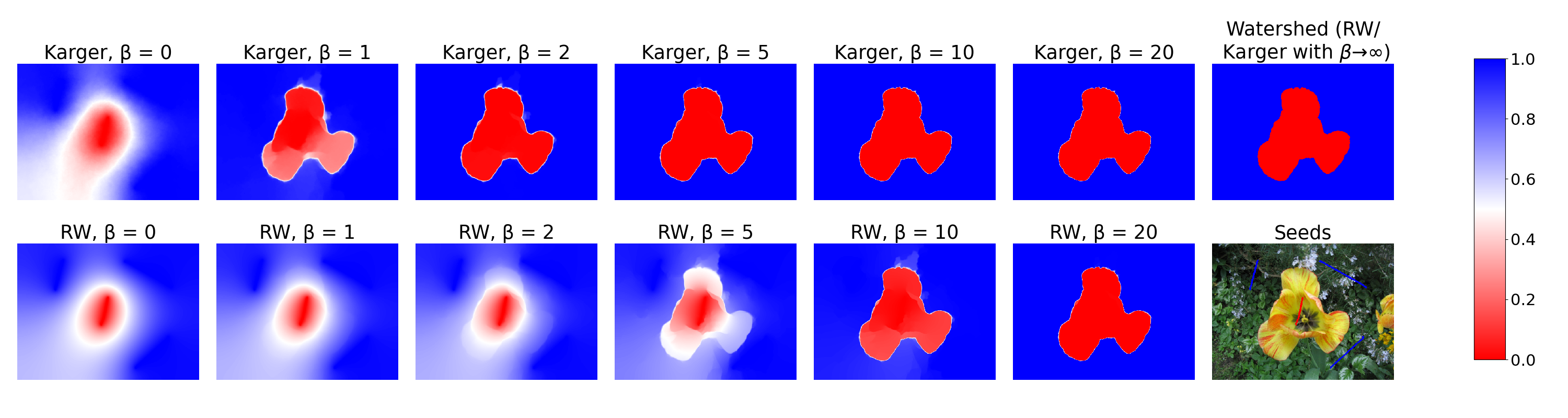
Figure 2: The probabilistic estimates of the Karger potential, compared to those of the random walker / harmonic energy minimization, for various graph edge weights.

In addition to the random walker, we also compare to the watershed segmentation, which has been used for both seeded segmentation [6] and semi-supervised learning [3]. This segmentation arises from a maximum spanning forest that separates the seeds [6]. If there is only one maximum spanning forest, both the Karger potential and the random walker potential converge to this segmentation as $\beta\to\infty$. The more general case of multiple maximum spanning forests is described by the Power Watershed framework [5, 30], which generalizes both the watershed and the random walker. This framework has two parameters, $q$ and $p$, and the case $q=2,p\to\infty$ is the limit of the random walker for $\beta\to\infty$, without any assumptions on the number of maximum spanning forests. When there is a unique maximum spanning forest, Power Watershed reduces to watershed; in particular, this is the case if all the edge weights are distinct. So we rounded the edge weights to 8 bits to artificially introduce the edges with equal weight that give Power Watershed the opportunity to shine relative to watershed. This leads to 256 different possible edge weights, exactly as in [5].

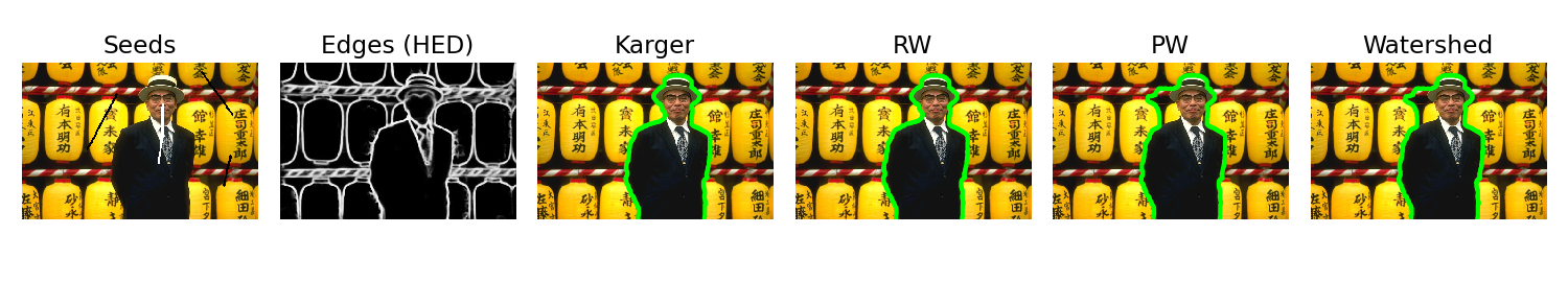
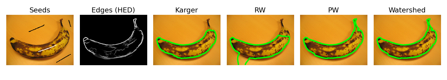
Figure 3: Some qualitative differences between Karger-type contractions, random walker / harmonic energy minimization and (Power) watershed. $\beta$ values are chosen optimally for each method.

	$\uparrow$ ARI	$\uparrow$ Acc [%]	$\downarrow$ VoI
Contraction	$0.82\pm 0.02$	$96.3\pm 0.6$	$0.24\pm 0.02$
RW	$0.82\pm 0.02$	$96.0\pm 0.6$	$0.25\pm 0.03$
Watershed	$0.83\pm 0.02$	$96.2\pm 0.5$	$0.24\pm 0.02$
Power WS	$0.83\pm 0.02$	$96.2\pm 0.5$	$0.24\pm 0.02$

Table 1: Seeded segmentation: Mean adjusted Rand index (ARI), accuracy (Acc) and variation of information (VoI) on the Grabcut dataset. RW = Random Walker, Power WS = Power Watershed with $q=2,p\to\infty$

Table 1 shows the results on the entire Grabcut dataset. We optimized $\beta$ by hand separately for each method and used the optimal values $\beta=10$ for the Karger potential and $\beta=20$ for the random walker. However, the performance of both algorithms is relatively stable within this range of values. The watershed algorithm does not depend on the value of $\beta$, as long as $\beta>0$. For Power Watershed, we used $\beta=10$ (though its dependency on $\beta$ is very low anyway). The reported error is the standard error of the mean over the dataset. We used 1000 runs of the seeded segmentation algorithm to approximate the Karger potential, which made the approximation error negligible in comparison.

We compare the four methods using the Adjusted Rand Index (ARI), their classification accuracy and the Variation of Information (VoI). For ARI and accuracy, higher is better, for VoI, lower is better. All metrics are calculated only over the unlabeled pixels.

Figure 3 shows an example of the seeds that were used, the output of the edge detection network and the resulting segmentations for each of the four methods, each at their optimal $\beta$ values. The results are for the most part very similar – the segmentations shown here have been selected because they are visibly different. In the first row, there are many strong edges and the (Power) watershed follows a different edge than the other methods. In the second row, some edges are missing and the four methods respond differently to this “leak”.

The output of the contraction algorithm is only an approximation of the true Karger potential but the error is so small that it does not visibly affect the contours of the segmentation.

Semi-supervised learning

Here, we used classical benchmark data from the training set of the USPS handwritten digits dataset [15, 24]. These are labeled $16\times 16$ grayscale images of digits from 0 to 9. We calculated all pairwise euclidean distances between the images and built the 10-nearest neighbors graph based on those. The graph weights were again computed using a radial basis function,

$$w_{ij}=\exp\left(-\beta\frac{d_{ij}^{2}}{a^{2}}\right)\,,$$ (14)

with $a:=\max_{\{i,j\}\in E}d_{ij}$, where $d_{ij}$ are the euclidean distances.

We used random subsets of different sizes as labeled vertices and left the remaining vertices to be labeled. For each size of the labeled set, we sampled 20 sets. Table 2 shows the accuracies over unlabeled data, averaged over these 20 samples. The errors are the standard errors of the sample mean. As before, the $\beta$ values were chosen individually for each method to maximize performance ($\beta=5$ for the random walker, $\beta=2$ for the contraction method).

Seeds	20	40	100	200
Contraction	$\mathbf{62.2}\pm 1.8$	$\mathbf{73.1}\pm 1.5$	$\mathbf{89.0}\pm 0.5$	$\mathbf{92.6}\pm 0.2$
RW	$53.7\pm 1.9$	$68.0\pm 1.2$	$87.7\pm 0.7$	$\mathbf{92.4}\pm 0.3$
Watershed	$54.3\pm 2.0$	$58.7\pm 1.9$	$74.3\pm 1.0$	$80.0\pm 0.9$
Power WS	$54.4\pm 2.0$	$59.0\pm 1.9$	$74.7\pm 1.0$	$80.8\pm 0.9$

Table 2: Graph-based semi-supervised learning: Accuracies in % on the USPS dataset. RW = Random Walker, Power WS = Power Watershed with $q=2,p\to\infty$

Throughout, we used the scikit-image implementation of the random walker [39] with slight adaptations to use the edge weights described above.

Results

In all our experiments, the new method based on the Karger potential performed comparably to the random walker / harmonic energy minimization. However, the new method has significantly better results in the semi-supervised learning setting with few labeled vertices.

6 Conclusion

We have shown that contraction algorithms that are continuous or that use only local properties of the edges cannot efficiently solve the $s$-$t$-mincut problem or the normalized cut problem to optimality. On the other hand, we have demonstrated that certain extensions of Karger’s algorithm can be successfully used for seeded segmentation and semi-supervised learning tasks: we have presented a contraction-based algorithm that performs as well as or better than the random walker / harmonic energy minimization, while having an asymptotic time complexity linear in the number of edges.

Future work might address the question whether contraction algorithms based on global properties can be useful for solving the $s$-$t$-mincut problem or whether our result can be extended to an even wider class of algorithms. Another open question is whether the $s$-$t$-contraction algorithm can find $s$-$t$-mincuts quickly on graphs that occur in practice, as opposed to the “malicious” artificial graphs we used in the impossibility proofs. Finally, Karger’s algorithm induces a distribution over spanning 2-forests, similarly to the distribution we describe in Section 4. Future research could shed more light on this distribution, for example whether it is uniquely well suited for finding minimum cuts or whether a Gibbs distribution would yield a result similar to Theorem 1.

• Appendix

  Appendix A Proofs for continuous contraction algorithms

  We will first prove theorem 2 for $s$-$t$-mincuts. Afterwards, we will give those parts of the proof for the normalized cut version that differ from the version for $s$-$t$-mincuts.

  Proof of theorem 2 for $s$-$t$-mincuts.

  Fix a value of $n$ and a continuous contraction algorithm, we will then construct a graph on which this algorithm finds an $s$-$t$-mincut with probability $\leq 2^{-n+3}$.

  Consider the graph $G$ in fig. 1 in the main paper, but with weight 1 for all edges and generalized to $n$ vertices (two of which are $s$ and $t$). We call the adjacency matrix of this graph $A$. Every $s$-$t$-cut of $G$ is minimal, and there are $2^{n-2}$ such $s$-$t$-cuts. So there must be at least one $s$-$t$-mincut, whose cut set we shall call $C$, that the contraction algorithm selects with probability $\leq 2^{-n+2}$.

  The idea of this proof is to slightly decrease the weights of all the edges in $C$. Because of continuity, we can do this in such a way that the probability of selecting $C$ does not change by much. Then the cut defined by $C$ will be the unique $s$-$t$-mincut in the modified graph but will still be selected with probability of order $2^{-n}$. What follows is a more rigorous version of this argument.

  We will write $p_{C}(\tilde{A})$ for the probability that the algorithm selects the cut $C$ on the graph with $n$ vertices and weighted adjacency matrix $\tilde{A}$. We know that $p_{C}(A)\leq 2^{-n+2}$. Our goal is to find an adjacency matrix $A^{\prime}$ for which $C$ is the unique $s$-$t$-mincut and $p_{C}(A^{\prime})\leq 2^{-n+3}$.

  First, we need to show that for a continuous contraction algorithm, $p_{C}(\tilde{A})$ is a continuous function of $\tilde{A}$. The definition of continuous contraction algorithms only states that the scores at each step need to be continuous function of the adjacency matrix. It’s unsurprising that this also leads to continuous overall probabilities of selecting given cuts. The details do not provide much insight and are shown separately as lemma 5.

  This continuity of $p_{C}(\tilde{A})$ means that for $\varepsilon:=2^{-n+2}$, there is a $\delta>0$ such that if $\left\lVert A-A^{\prime}\right\rVert_{\infty}\leq\delta$ for some $A^{\prime}$, then $\left\lvert p_{C}(A)-p_{C}(A^{\prime})\right\rvert\leq\varepsilon$.

  So we define the graph $G^{\prime}$ with adjacency matrix $A^{\prime}$ by setting the weights of the edges in the cut set $C$ to $1-\delta$ and leaving the other weights at $1$. Then $\left\lVert A-A^{\prime}\right\rVert_{\infty}=\delta$, so

  $$\left\lvert p_{C}(A)-p_{C}(A^{\prime})\right\rvert\leq\varepsilon=2^{-n+2}$$

  This means that the probability of finding the cut $C$ in the new graph $G^{\prime}$ is

  $$p_{C}(A^{\prime})\leq p_{C}(A)+\varepsilon\leq 2^{-n+2}+2^{-n+2}=2^{-n+3}$$

  At the same time, $C$ is the unique $s$-$t$-mincut of $G^{\prime}$. Every $s$-$t$-cut has a cut set with the same cardinality and $C$ is the only one which contains only edges that have weight $1-\delta$ — every other cut set contains some edges with weight 1.

  This means that on $G^{\prime}$, the contraction algorithm has only an exponentially low probability of finding any $s$-$t$-mincut, as claimed. ∎

  Proof of theorem 2 for normalized cuts.

  Instead of the graph from fig. 1 in the main paper that we used in the previous proof, let $G$ be a complete unweighted graph on $n$ vertices. We will show that in this graph, every cut is a normalized cut.

  In a complete unweighted graph, we always have

  $$w(A,B)=\sum_{a\in A,b\in B}w_{ab}=|A|\cdot|B|-|A\cap B|$$

  (the last term is necessary because there are no self-loops). Therefore, with $k:=|A|$, we get

  $$w(A,A^{c}) =k(n-k)$$

  $$w(A,V) =k(n-1)$$

  $$w(A^{c},V) =(n-k)(n-1)$$

  So the normalized cut cost of the cut $(A,A^{c})$ is

  $$\begin{split}\operatorname{ncut}(A,A^{c})&=\frac{w(A,A^{c})}{w(A,V)}+\frac{w(A,A^{c})}{w(A^{c},V)}=\frac{k(n-k)}{k(n-1)}+\frac{k(n-k)}{(n-k)(n-1)}\\ &=\frac{(n-k)+k}{n-1}=\frac{n}{n-1}\end{split}$$

  for each of the $2^{n-1}$ possible cuts. This means that there are $2^{n-1}$ normalized cuts, and the algorithm must assign probability $\leq 2^{-n+1}$ to at least one of them.

  From here on the proof procedes like that for $s$-$t$-mincuts: if the weights are slightly perturbed, there will be a unique normalized cut, but its probability will still be close to $2^{-n+1}$. We therefore don’t repeat the details. ∎

  To make working with weighted adjacency matrices easier, we consider every graph to be fully connected for the following Lemma. Non-existent edges are instead treated as edges with weight zero.

  Lemma 5.

  Let $C$ be a fixed set of edges of the complete graph on $n$ vertices. Let $p_{C}(A)$ be the probability that a given continuous contraction algorithm does not contract any edges from $C$ when run on the graph with $n$ vertices and weighted adjacency matrix $A$. Then $p_{C}$ is a continuous function.

  Note that we don’t require $C$ to be a cut set and that here, $p_{C}(A)$ does not always denote the probability that $C$ is the chosen cut. This makes the proof more concise and is a strict generalization: if $C$ happens to be a cut set for some adjacency matrix $A$, then $p_{C}(A)$ will be the probability that $C$ is the final chosen cut.

  Proof.

  Let $e_{1},\ldots,e_{n-2}$ be an arbitrary but fixed set of edges. We will show that the probability $p(e_{1},\ldots,e_{n-2})$ that the algorithm contracts $e_{1},\ldots,e_{n-2}$ in that order is a continuous function of $A$. Then the claim follows because $p_{C}(A)$ is simply the sum of these probabilities over all $(n-2)$-tuples of edges that don’t contain edges from $C$.

  We prove the claim in two steps:

  1. Let $C_{k}(A)$ for $k\in\{1,\ldots,n-2\}$ be the adjacency matrix that is reached from starting with $A$ and contracting $e_{1},\ldots,e_{k}$. We will show that $C_{k}(A)$ is a continuous function for all $k$.

  2. We then show that $p(e_{1},\ldots,e_{n-2})$ is a continuous function of the partially contracted adjacency matrices $C_{1}(A),\ldots,C_{n-2}(A)$

  It will then follow that $p(e_{1},\ldots,e_{n-2})$ and thus $p_{C}$ is a continuous function of $A$, as a composition of continuous functions.

  For the first step, note that contracting an edge sets an entry in the adjacency matrix to zero and adds its previous value to another entry. This means that each entry of $C_{1}(A)$ is either zero (for all $A$) or a certain sum of entries of $A$. The structure of the sum is determined by $e_{1}$ and does not depend on $A$. Therefore, $C_{1}$ is a continuous function of $A$. Each entry in $C_{2}(A)$ is zero or a sum of entries in $C_{1}(A)$ and therefore a continuous function of $C_{1}(A)$, which makes it a continuous function of $A$ by composition. By induction it follows that all $C_{k}$ are continuous functions of $A$.

  For the second step, we write $p(e_{1},\ldots,e_{n-2})$ as

  $$p(e_{1},\ldots,e_{n-2})=\prod_{k=1}^{n-2}\frac{\mathcal{W}(e_{k};C_{k}(A))}{\sum_{e}\mathcal{W}(e;C_{k}(A))}$$ (15)

  the sum over $e$ is over all the edges at that step; which summands appear depends only on $e_{1},\ldots,e_{n-2}$ and not on $A$. The scores $\mathcal{W}$ that appear are by definition continuous in their second argument $C_{k}(A)$. Since $C_{k}(A)$ is continuous in $A$ and the entire expression is clearly continuous in the scores, $p(e_{1},\ldots,e_{n-2})$ is continuous in $A$ as claimed. ∎

  Appendix B Proofs for local contraction algorithms

  We will first prove theorem 3 for $s$-$t$-mincuts. The approximability result from corollary 4 and the result for normalized cuts will then follow easily.

  Proof of theorem 3 for $s$-$t$-mincuts.

  The graphs $G_{n}$ we will use consist of $n$ copies of each of three different subgraphs, shown in fig. 4. As an example, a schematic version of $G_{2}$ is shown in fig. 5. Each of the colored boxes contains one subgraph, each of the three types occurs twice. The different box colors denote the three different types. The last two types only differ in their orientation but we will treat them separately. The general graph $G_{n}$ simply has $n$ instead of two copies of each subgraph.

  

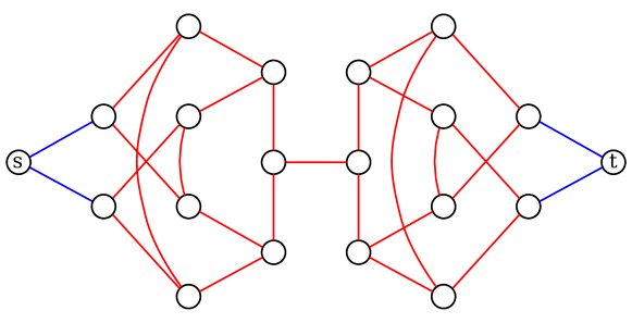
  (a) Band of type A

  

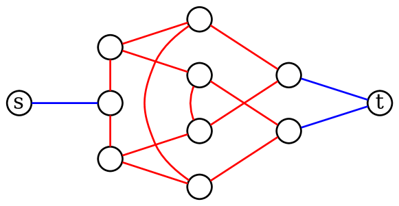
  (b) Band of type B

  

  (c) Band of type C

  Figure 4: The three different “bands” used in $G_{n}$

  

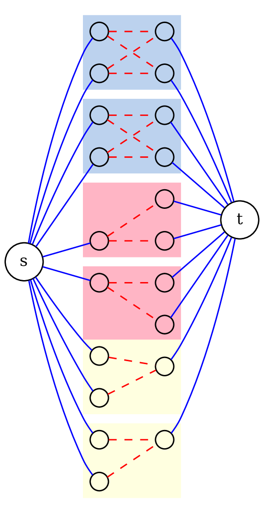
  Figure 5: The unweighted graph $G_{2}$. The idea is still the same as for the simpler example from fig. 1 in the main paper. But the short parallel paths between $s$ and $t$ have now been replaced by “bands”, our name for the subgraphs in colored boxes. This construction ensures that it is impossible to find “safe” edges for contraction based only on local properties. The bands are only hinted at here, the full bands are shown in fig. 4. Blue corresponds to type A, red to B, yellow to C.

  We call each such subgraph, including the blue edges that connect it to $s$ and $t$, a band. There are $3n$ bands, $n$ of each type. We say that a band has been touched if one of the edges belonging to it has been contracted. Clearly, every band has to be touched at some point during the contraction process.

  One of the key ideas of the proof is that $G_{n}$ contains many edges that have isomorphic neighborhoods, but some of which are part of the $s$-$t$-mincut while others are not. A local contraction algorithm assigns the same score to each of these edges with isomorphic neighborhoods. This will give us a lower bound on the contraction probability of edges included in the $s$-$t$-mincut cut set in any particular step.

  All of the edges in $G_{n}$ belong to one of three isomorphism classes of neighborhoods, which we call red, $s$-blue and $t$-blue. These neighborhoods are shown in fig. 6.

  

  (a) Red neighborhood

  

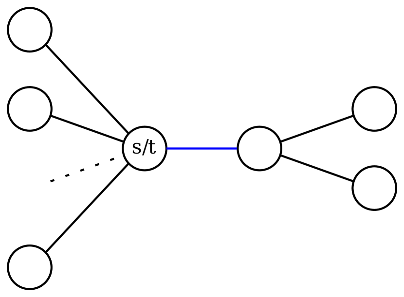
  (b) Blue neighborhood

  Figure 6: The different neighborhoods that occur in $G_{n}$. $s$-blue and $t$-blue are both shown in fig. 6(b) because they differ only in whether they contain the node $s$ or $t$.

  The blue neighborhood classes depend on the degree of $s$ ($t$) which is a function of $n$. We will call an edge $s$-blue ($t$-blue) if its neighborhood fits the schema from fig. 6(b), no matter the degree of $s$ ($t$). In a fixed graph, all $s$-blue ($t$-blue) edges have isomorphic neighborhoods. That the same is not true across graphs does not matter for our purposes.

  All the edges are colored according to their neighborhood (blue and red) in fig. 4. During the contraction process, other neighborhoods may of course arise.

  The unique $s$-$t$-mincut of $G_{n}$ cuts the red edge in the middle of each band of type A and the blue edges on the side where there is only one of them in bands of type B and C. The contraction algorithm will find this minimum cut iff it does not contract any of these edges. So we will say a contraction is “wrong” or a “mistake” if it contracts one of these edges belonging to the $s$-$t$-mincut.

  We will now prove some useful statements:

  1. In an untouched band, all edges are either red, $s$-blue or $t$-blue, with each edge belonging to the same type as in the original graph $G_{n}$.

     Proof.

     It’s clear that contractions of red edges in one band don’t influence other bands. If a blue edge is contracted, this can change the degree of $s$ or $t$ but has no influence on other bands apart from that. ∎

  2. If at most $\frac{n}{2}$ bands have been touched, then the probability that contracting a blue or red edge is wrong is $p(\text{wrong}|\text{red or blue})\geq\frac{1}{118}$.

     Proof.

     There are still at least $\frac{n}{2}$ untouched bands of all three types. Each type contains a red edge, an $s$-blue edge or a $t$-blue edge that mustn’t be contracted respectively (as per the statement proven just above). So there are at least $\frac{n}{2}$ wrong red edges, $\frac{n}{2}$ wrong $s$-blue edges and $\frac{n}{2}$ wrong $t$-blue edges.

     Because all red edges have the same neighborhood, the local contraction algorithm assigns the same score to all red edges. The same is true for $s$-blue edges and for $t$-blue edges. So we have

     $$p(\text{wrong}|\text{red})=\frac{\#\text{wrong red edges}}{\#\text{red edges}}\geq\frac{\#\text{wrong red edges}}{\#\text{total edges}}\geq\frac{n/2}{59n}=\frac{1}{118}$$

     and similarly $p(\text{wrong}|s\text{-blue})\geq\frac{1}{118}$ and the same for $t$. This means that $p(\text{wrong}|\text{red or blue})$ is bounded by

     $$\begin{split}p(\text{wrong}|\text{r or b})&=\frac{p(\text{wrong}|\text{r})p(\text{r})+p(\text{wrong}|s\text{-b})p(s\text{-b})+p(\text{wrong}|t\text{-b})p(t\text{-b})}{p(\text{r})+p(s\text{-b})+p(t\text{-b})}\\ &\geq\frac{\frac{1}{118}\cdot p(\text{r})+\frac{1}{118}\cdot p(s\text{-b})+\frac{1}{118}\cdot p(t\text{-b})}{p(\text{r})+p(s\text{-b})+p(t\text{-b})}\\ &=\frac{1}{118}\end{split}$$

     $p(r)$, $p(s\text{-b})$ and $p(t\text{-b})$ are what can be influenced by the choice of the scoring function $\mathcal{W}$ but these terms cancel as we can see. ∎

  We will now prove inductively that contracting an edge in $k$ different bands without contracting any wrong edges happens with probability $\leq\left(\frac{117}{118}\right)^{k}$ for $k\leq\frac{n}{2}$:

  $$p_{k}:=p\left(\text{no mistakes}\mid k\text{ bands touched}\right)\leq\left(\frac{117}{118}\right)^{k}$$

  Proof.

  $k=0$

  Nothing to show.

  $k\to k+1$

  The probability of not making any mistakes until $k+1$ bands have been touched is the probability $p_{k}$ of correctly touching the first $k$ bands times the probability of not making a mistake while touching the final band.

  From statement 1 proven above, we know that to touch a new band, a red, $s$-blue or $t$-blue edge will have to be contracted at some point. From statement 2 we know that the probability of making a mistake on that single contraction is at least $\frac{1}{118}$. Additional contractions may be made, but they cannot decrease the total probability of making any mistake. So

  $$p_{k+1}\leq\left(\frac{117}{118}\right)^{k}\cdot\frac{117}{118}=\left(\frac{117}{118}\right)^{k+1}$$

  which proves the claim for $k+1$.

  ∎

  Since all bands have to be touched eventually, we can apply this statement with $k=\frac{n}{2}$. So the success probability is at most $\left(\frac{117}{118}\right)^{n/2}$ which is exponentially low in the number of vertices, $36n+2$, as claimed. ∎

  Proof of corollary 4.

  Since the $s$-$t$-mincut has cost $3n$, an $\alpha$-minimal cut may be worse than the mincut by at most $3n(\alpha-1)$. Every wrong contraction in an untouched band increases the cost of the best cut that is still possible by at least 1 (because there is only one unique way to optimally cut each band). So to find an $\alpha$-minimal $s$-$t$-cut, at most $3n(\alpha-1)$ wrong contractions may be made in untouched bands.

  As there are $3n$ bands, at least $3n-3n(\alpha-1)=(6-3\alpha)n$ contractions in different bands must be made without mistakes.

  We showed in the proof of theorem 3 that making contractions in $k$ different bands without mistakes (with $k\leq\frac{n}{2}$) happens with probability $\leq\left(\frac{117}{118}\right)^{k}$. If $\alpha<2$, then $6-3\alpha>0$, and therefore we can apply this result with $k=(6-3\alpha)n$ and see that the probability of correctly contracting edges in the required number of bands is exponentially low in $n$.

  Therefore, the probability that mistakes are made in only $3n(\alpha-1)$ bands is exponentially low, and thus also the probability of finding an $\alpha$-minimal $s$-$t$-cut. ∎

  Proof of theorem 3 for normalized cuts.

  It suffices to show that the $s$-$t$-mincut in $G_{n}$ is also the normalized cut for large $n$. The $s$-$t$-mincut cuts $3n$ edges. Because the partitions are perfectly balanced in terms of internal edge weights, only cuts that cut fewer edges than that can have a lower normalized cut cost. In particular, any such cut could not separate $s$ and $t$. One of its partitions could therefore be no larger than one of the bands between $s$ and $t$. But the normalized cut cost of such a cut approaches 1 for large $n$, whereas the ncut cost of the $s$-$t$-mincut is always $2\cdot\frac{3n}{2\cdot 28n+3n}=\frac{6n}{59n}=\frac{6}{59}$. So the $s$-$t$-mincut is indeed also the normalized cut for large $n$. ∎

  Appendix C Implementation of the seeded contraction algorithm

  For unweighted graphs, Karger’s algorithm can be implemented in $\mathcal{O}(m)$ time as follows [19]: First, a random permutation of all $m$ edges is generated which takes $\mathcal{O}(m)$ time. Afterwards, edges are contracted in the chosen order until only two vertices remain. If an edge has already been removed by previous contractions, it is skipped. [19] also describes how this method can be generalized to weighted graphs. The only change is in how to generate the permutation of edges to give different probabilities to different permutations.

  To keep track of when to stop and of the current segmentation at each step, we use a union-find data structure. Keeping this structure up to date increases the runtime to $\alpha(n)\mathcal{O}(m)$ [38] where $n$ is the number of vertices and $\alpha(n)$ the inverse Ackermann function. But since $\alpha(n)<5$ for all practical values of $n$, this theoretical increase has no practical relevance.

  Two modifications are necessary to adapt this implementation to the seeded contraction algorithm: first, we initialize the union-find data structure such that nodes with the same seed are in the same cluster from the beginning. This is possible with a linear scan over all nodes in $\mathcal{O}(n)$.

  Second, we keep a boolean vertex property updated that denotes whether a node is already labeled (i.e. in the cluster of a seed node) or not. Whenever we come to an edge connecting two nodes that are already labelled, we skip it instead of merging these nodes. This ensures that no seeds with different labels end up in the same cluster and each node has a well-defined label at the end. These extensions do not increase the runtime of processing one edge beyond $\mathcal{O}(1)$, so the total runtime of the algorithm stays $\mathcal{O}(m\alpha(n))$.

  Appendix D Details on experiments

  D.1 Metrics

  We used three common metrics to evaluate performance in the Grabcut experiment: the adjusted Rand index (ARI), variation of information (VoI) and accuracy.

  The (unadjusted) Rand index is defined as the accuracy on the space of pairs of samples, in the following sense: count the number TP of pairs of samples that are correctly put in the same cluster (true positives) and the number TN of pairs of samples that are correctly put in different clusters (true negatives). Then the Rand index is $\frac{TP+TN}{{n\choose 2}}$ for $n$ samples, where ${n\choose 2}$ is the total number of pairs of samples.

  The adjusted Rand index renormalizes the Rand index such that it is 1 for a perfect clustering and has expected value 0 for a random clustering, independently of the number of clusters. This is done by correcting for chance with

  $$\text{ARI }=\frac{\text{RI }-\mathbb{E}[\text{RI}]}{1-\mathbb{E}[\text{RI}]}$$

  where RI is the Rand index and the expectation is over permutations of the assigned labels. The expected value of 0 makes the ARI easy to interpret compared to the unadjusted Rand index, for which even random clusterings can have a positive expected value.

  The variation of information between two variables $X$ and $Y$ can be defined as

  $$\operatorname{VI}(X;Y):=H(X|Y)+H(Y|X)$$

  where $H(X|Y)$ is the conditional Shannon entropy. To get a clustering metric, we let $X$ and $Y$ be the different labelings (in our case ground truth and the labeling to be evaluated). The joint distribution over $X$ and $Y$ is defined by picking samples uniformly at random.

  D.2 Parameters

  In both experiments, we optimized the $\beta$ parameter by hand to maximize the performance according to the metrics we used separately for each method. In the Grabcut experiment multiple metrics were used, but they all reached their maximum at the same $\beta$ value of those we tested.

  In both experiments, we first found a reasonable range of $\beta$ values and then tested ten different values within these ranges. For the Grabcut experiment, this range was $\beta=5$ to $\beta=100$, for the USPS experiment it was $\beta=1$ to $\beta=20$.

  D.3 Empirical runtimes

  For a complete run on both datasets (Grabcut and USPS), the new Karger-based algorithm takes about 20 minutes, the random walker takes about 5 minutes and watershed 9 minutes. All of these are wall clock times when running on 6 CPU cores. The random walker implementation is the one used in SciPy, the other algorithms were implemented by us in Julia. Their runtimes could probably be decreased with a more efficient implementation.

References

- [1] András A. Benczúr and David R. Karger. Approximating - minimum cuts in time. In STOC ’96, 1996.
- [2] Y.Y. Boykov and M.-P. Jolly. Interactive graph cuts for optimal boundary region segmentation of objects in N-D images. In Proceedings Eighth IEEE International Conference on Computer Vision, 2001.
- [3] A. Challa, S. Danda, B. S. D. Sagar, and L. Najman. Watersheds for Semi-Supervised Classification. IEEE Signal Processing Letters, 2019.
- [4] Michael B. Cohen, Rasmus Kyng, Gary L. Miller, Jakub W. Pachocki, Richard Peng, Anup B. Rao, and Shen Chen Xu. Solving SDD linear systems in nearly time. In Proceedings of the Forty-Sixth Annual ACM Symposium on Theory of Computing, 2014.
- [5] Camille Couprie, Leo Grady, Laurent Najman, and Hugues Talbot. Power Watershed: A Unifying Graph-Based Optimization Framework. IEEE Transactions on Pattern Analysis and Machine Intelligence, 2011.
- [6] J. Cousty, G. Bertrand, L. Najman, and M. Couprie. Watershed cuts: Minimum spanning forests and the drop of water principle. IEEE Transactions on Pattern Analysis and Machine Intelligence, 2009.
- [7] Enrique Fita Sanmartin, Sebastian Damrich, and Fred A Hamprecht. Probabilistic Watershed: Sampling all spanning forests for seeded segmentation and semi-supervised learning. In Advances in Neural Information Processing Systems, 2019.
- [8] Paweł Gawrychowski, Shay Mozes, and Oren Weimann. Minimum cut in time. 2019.
- [9] Y. Gdalyahu, D. Weinshall, and M. Werman. Self-organization in vision: Stochastic clustering for image segmentation, perceptual grouping, and image database organization. IEEE Transactions on Pattern Analysis and Machine Intelligence, 2001.
- [10] Mohsen Ghaffari, Krzysztof Nowicki, and Mikkel Thorup. Faster algorithms for edge connectivity via random 2-out contractions. In Proceedings of the Thirty-First Annual ACM-SIAM Symposium on Discrete Algorithms, 2020.
- [11] L. Grady. Random Walks for Image Segmentation. IEEE Transactions on Pattern Analysis and Machine Intelligence, 2006.
- [12] Leo J. Grady and Jonathan R. Polimeni. Discrete Calculus. Springer London, London, 2010.
- [13] D.M. Greig, B.T. Porteous, and Allan Seheult. Exact Maximum A Posteriori Estimation for Binary Images. Journal of the Royal Statistical Society, Series B, 1989.
- [14] Varun Gulshan, Carsten Rother, Antonio Criminisi, Andrew Blake, and Andrew Zisserman. Geodesic star convexity for interactive image segmentation. In 2010 IEEE Computer Society Conference on Computer Vision and Pattern Recognition, 2010.
- [15] J.J. Hull. A database for handwritten text recognition research. IEEE Transactions on Pattern Analysis and Machine Intelligence, 1994.
- [16] David R. Karger. Global min-cuts in RNC, and other ramifications of a simple min-cut algorithm. In Proceedings of the Fourth Annual ACM-SIAM Symposium on Discrete Algorithms, 1993.
- [17] David R. Karger. Minimum cuts in near-linear time. Journal of the ACM, 2000.
- [18] David R. Karger and Clifford Stein. An algorithm for minimum cuts. In Proceedings of the Twenty-Fifth Annual ACM Symposium on Theory of Computing, 1993.
- [19] David R. Karger and Clifford Stein. A new approach to the minimum cut problem. Journal of the ACM, 1996.
- [20] Jonathan A. Kelner, Yin Tat Lee, Lorenzo Orecchia, and Aaron Sidford. An Almost-Linear-Time Algorithm for Approximate Max Flow in Undirected Graphs, and its Multicommodity Generalizations. In Proceedings of the 2014 Annual ACM-SIAM Symposium on Discrete Algorithms. 2013.
- [21] V. Kolmogorov and R. Zabin. What energy functions can be minimized via graph cuts? IEEE Transactions on Pattern Analysis and Machine Intelligence, 2004.
- [22] I. Koutis, G. L. Miller, and R. Peng. Approaching Optimality for Solving SDD Linear Systems. In 2010 IEEE 51st Annual Symposium on Foundations of Computer Science, 2010.
- [23] I. Koutis, G. L. Miller, and R. Peng. A Nearly- Time Solver for SDD Linear Systems. In 2011 IEEE 52nd Annual Symposium on Foundations of Computer Science, 2011.
- [24] Yann LeCun, Bernhard E. Boser, John S. Denker, Donnie Henderson, R. E. Howard, Wayne E. Hubbard, and Lawrence D. Jackel. Handwritten Digit Recognition with a Back-Propagation Network. In Advances in Neural Information Processing Systems. 1990.
- [25] Lei Li, Hongbo Fu, and Chiew-Lan Tai. Fast Sketch Segmentation and Labeling With Deep Learning. IEEE Computer Graphics and Applications, 2019.
- [26] Zhe Liu, Yu-Qing Song, Victor S. Sheng, Liangmin Wang, Rui Jiang, Xiaolin Zhang, and Deqi Yuan. Liver CT sequence segmentation based with improved U-Net and graph cut. Expert Systems with Applications, 2019.
- [27] Antonio Molina Lovett and Bryce Sandlund. A Simple Algorithm for Minimum Cuts in Near-Linear Time. In SWAT, 2020.
- [28] Fang Lu, Fa Wu, Peijun Hu, Zhiyi Peng, and Dexing Kong. Automatic 3D liver location and segmentation via convolutional neural network and graph cut. International Journal of Computer Assisted Radiology and Surgery, 2017.
- [29] Suvadip Mukherjee, Xiaojie Huang, and Roshni R. Bhagalia. Lung nodule segmentation using deep learned prior based graph cut. In 2017 IEEE 14th International Symposium on Biomedical Imaging (ISBI 2017), 2017.
- [30] Laurent Najman. Extending the power watershed framework thanks to -convergence. SIAM Journal on Imaging Sciences, 2017.
- [31] P. Nardelli, D. Jimenez-Carretero, D. Bermejo-Pelaez, G. R. Washko, F. N. Rahaghi, M. J. Ledesma-Carbayo, and R. San José Estépar. Pulmonary Artery–Vein Classification in CT Images Using Deep Learning. IEEE Transactions on Medical Imaging, 2018.
- [32] Simon Niklaus. A reimplementation of HED using PyTorch. https://github.com/sniklaus/pytorch-hed, 2018.
- [33] Bo Pang and Lillian Lee. A Sentimental Education: Sentiment Analysis Using Subjectivity Summarization Based on Minimum Cuts. In Proceedings of the 42nd Annual Meeting of the Association for Computational Linguistics (ACL-04), 2004.
- [34] Carsten Rother, Vladimir Kolmogorov, and Andrew Blake. “GrabCut”: Interactive foreground extraction using iterated graph cuts. In ACM SIGGRAPH 2004 Papers, 2004.
- [35] J. Sherman. Nearly Maximum Flows in Nearly Linear Time. In 2013 IEEE 54th Annual Symposium on Foundations of Computer Science, 2013.
- [36] Jianbo Shi and J. Malik. Normalized cuts and image segmentation. IEEE Transactions on Pattern Analysis and Machine Intelligence, 2000.
- [37] Daniel A. Spielman and Shang-Hua Teng. Nearly-linear time algorithms for graph partitioning, graph sparsification, and solving linear systems. In Proceedings of the Thirty-Sixth Annual ACM Symposium on Theory of Computing, 2004.
- [38] Robert E. Tarjan and Jan van Leeuwen. Worst-case Analysis of Set Union Algorithms. Journal of the ACM, 1984.
- [39] Stéfan van der Walt, Johannes L. Schönberger, Juan Nunez-Iglesias, François Boulogne, Joshua D. Warner, Neil Yager, Emmanuelle Gouillart, and Tony Yu. Scikit-image: Image processing in Python. PeerJ, 2014.
- [40] Z. Wu and R. Leahy. An optimal graph theoretic approach to data clustering: Theory and its application to image segmentation. IEEE Transactions on Pattern Analysis and Machine Intelligence, 1993.
- [41] Saining Xie and Zhuowen Tu. Holistically-Nested Edge Detection. In 2015 IEEE International Conference on Computer Vision (ICCV), 2015.
- [42] Ning Xu, Brian Price, Scott Cohen, Jimei Yang, and Thomas S. Huang. Deep Interactive Object Selection. In Proceedings of the IEEE Conference on Computer Vision and Pattern Recognition, 2016.
- [43] Yulun Zhang, Chen Fang, Yilin Wang, Zhaowen Wang, Zhe Lin, Yun Fu, and Jimei Yang. Multimodal Style Transfer via Graph Cuts. In Proceedings of the IEEE/CVF International Conference on Computer Vision, 2019.
- [44] Xiaojin Zhu, Zoubin Ghahramani, and John Lafferty. Semi-supervised learning using Gaussian fields and harmonic functions. In Proceedings of the Twentieth International Conference on Machine Learning, 2003.
-