Cooper problem in a cuprate lattice

Abstract

We solve the Cooper problem in a cuprate lattice by utilizing a three-band model. We determine the ground state of a Cooper pair for repulsive on-site interactions, and demonstrate that the corresponding wave function has an orbital $d_{x^{2}-y^{2}}$ symmetry. We discuss the influence of next-nearest-neighbor tunneling on the Cooper pair solution, in particular the necessity of next-nearest-neighbor tunneling for having d-wave pairs for hole-doped systems. We also propose experimental signatures of the d-wave Cooper pairs for a cold-atom system in a cuprate lattice.

I introduction

A cuprate lattice is a modified two-dimensional Lieb lattice that is characterized by a square unit cell with three sites Lieb_paper ; Lieb_lattice_Nita ; Plakida_HTc_Book ; Leggett_Cuprates ; see Fig. 1. In terms of single particle terms, we include potential energies for the p- and d-orbitals, which have different values. The difference of these potential energies modifies the charge-transfer energy. Furthermore, we include a tunneling energy between the p-orbitals. The single-particle energy spectrum of this lattice has two dispersive bands and one nearly flat band in between. A large charge-transfer energy provides a gap between the dispersive upper band and the other two bands, where the dispersion of the latter is due to the tunneling between p-orbitals, which is assumed to be smaller than the other energies; see Figs. 2(a) and 2(c). As we describe below, we will also assume the on-site interaction of two particles to be different on p- and d-orbitals. Realizations and proposals for this and related lattices have been reported for cold atoms BEC_book ; trapping_atoms ; Lieb_optical_1 ; Lieb_optical_2 ; Lieb_optical_3 ; Lieb_atomic_1 ; Lieb_atomic_2 and photonic systems Lieb_photonic_1 as well as for solid-state systems Lieb_material_1 ; Lieb_material_2 . Phenomena that are associated with flat-band or three-band systems have been reported in Refs. Lieb_lattice_Flach ; Flach_flat_band_review ; FB_1 ; FB_2 ; FB_3 ; FB_4 ; FB_5 ; FB_6 .

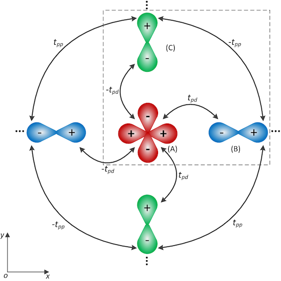
Figure 1: Sketch of the two-dimensional cuprate lattice in real space. The unit cell is shown by a dashed square, including a $d_{x^{2}-y^{2}}$ orbital configuration on the A-site, a $p_{x}$ orbital on the B-site, and a $p_{y}$ orbital on the C-site. The nearest-neighbor hopping is shown by $t_{pd}$ and the next-nearest-neighbor hopping is shown by $t_{pp}$.

The namesake realization of this lattice are the cuprate materials, in particular the copper-oxide layers, which are modeled as a cuprate lattice described above. These layers of Cu and O atoms directly realize the lattice displayed in Fig. 1, where the Cu atoms are represented as a $d_{x^{2}-y^{2}}$ orbital, and O atoms as $p_{x}$ and $p_{y}$ orbitals. It is assumed that the $\mathrm{Cu}\mathrm{O}_{2}$ layers are the location of the electron pairs, and therefore contain the origin of superconductivity High_Tc_Handbook ; Lynn_HTc_Book ; Anderson_Cuprate_Book ; Uchida_HTc_Book . The mechanism of pairing is under debate, with competing proposals reported in Refs. HTc_Phonon_1 ; HTc_Phonon_2 ; HTc_Phonon_3 ; HTc_Phonon_4 ; HTc_Phonon_5 ; HTc_Magnon_1 ; High_Tc_pairing_mechanism_1 ; HTc_Plasmon_1 ; HTc_Plasmon_2 ; HTc_Plasmon_3 ; HTc_Plasmon_4 ; Alexandrov_Hubbard_repulsive . ARPES measurements have provided insight into the Fermi surface geometry in the relevant regime Plakida_HTc_Book ; Leggett_Cuprates ; Alexandrov_Book ; ARPES_1 ; ARPES_2 ; ARPES_3 ; ARPES_4 ; ARPES_5 ; Starfish , which can be captured by the three-band model; see see Fig. 2(b) and 2(d). Numerous theoretical studies on determining the ground state of the interacting cuprate problem have been reported; see, e.g., Refs. Spalek_HTc_Cuprate ; Spalek_t_J_model ; Spalek_t_J_U_model ; H_K_model ; DMET_1 ; DMET_2 ; AFQMC ; iPEPS ; DMRG ; FLEX_DMFT .

In the study of conventional superconductors, the Cooper problem and its solution constituted a defining insight that advanced the understanding of superconductivity in general. In its original formulation, the Cooper problem assumes an effective electron-electron attraction due to the dominance of the electron-phonon interaction over the screened Coulomb repulsion, leading to a Cooper pair with an orbital s-wave symmetry Leggett_Cuprates ; Cooper_paper ; Goodstein_1 ; Abrikosov_book_metals ; Tinkham_1 ; Aschcroft_Mermin_1 . This insight paved the way for the subsequent development of BCS theory. Extensions of the Cooper problem to three-body systems have been presented in Refs. Sanayei_1 ; Sanayei_2 .

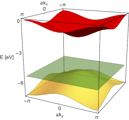
(a)      (b)

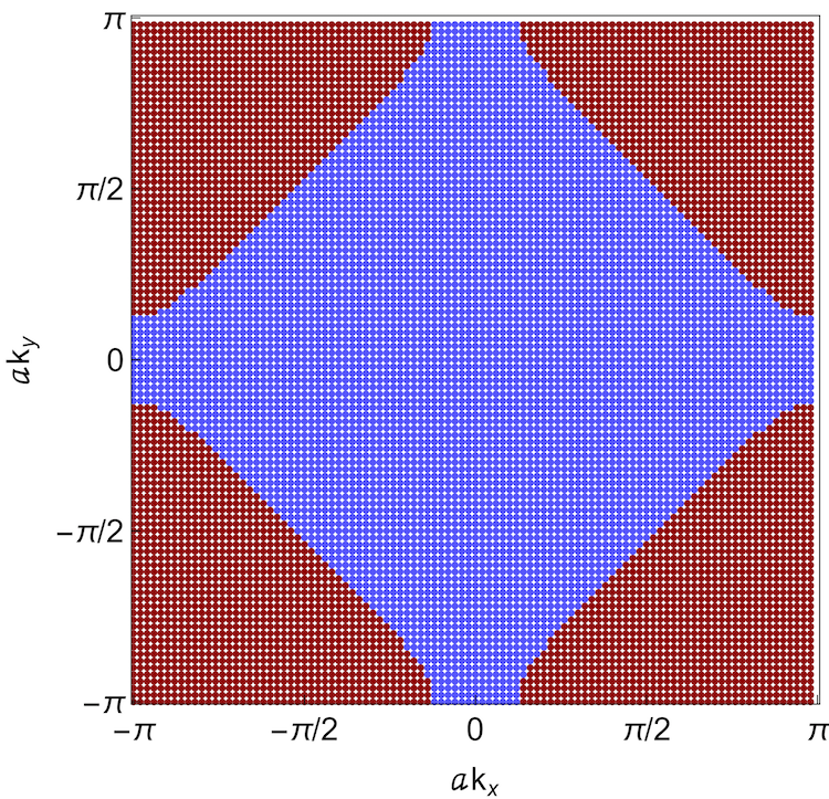
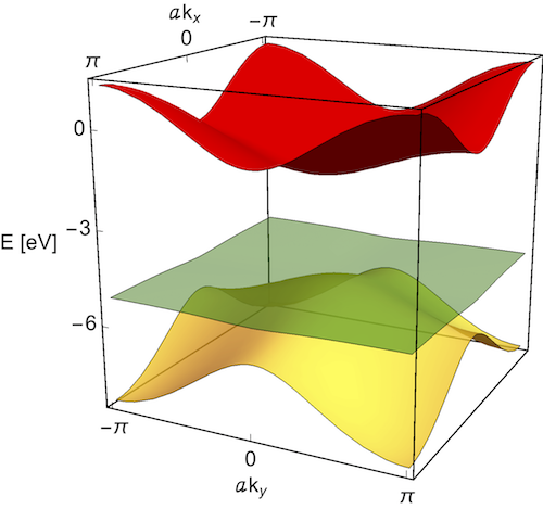
(c)      (d)

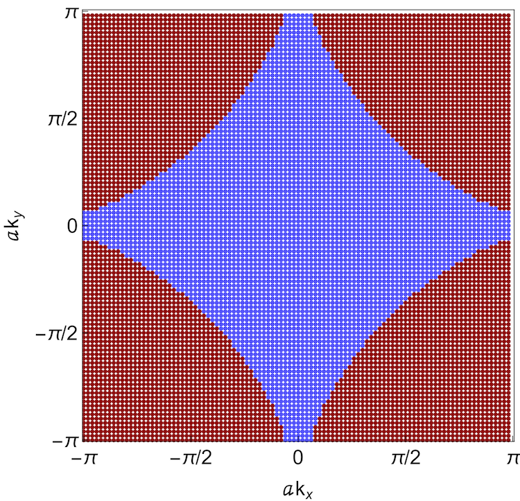
Figure 2: Electronic band structure and Fermi surface of a cuprate lattice in the first Brillouin zone for $V_{dp}=3.45\text{ eV}$ and $t_{pd}=1.13\text{ eV}$: (a) Band structure for $t_{pp}=0$; (b) the corresponding Fermi surface for $\mu\approx-0.679\text{ eV}$; (c) band structure for $t_{pp}=0.8\text{ eV}$; and (d) the corresponding Fermi surface for $\mu\approx-0.679\text{ eV}$ in the upper band. The two lower bands are filled. For $t_{pp}\neq 0$ the flat band is deformed, and the curvature of the dispersive bands is changed. Blue and red dots in panels (b) and (d) correspond to the occupied and unoccupied states, respectively.

In this paper we solve the Cooper problem for a cuprate lattice. The Cooper problem is intrinsically suitable for the weak-coupling limit of a Fermi system, because a nearly-intact Fermi sea is assumed. Our proposal aims primarily at ultracold atom systems, specifically Fermi mixtures in cuprate optical lattices, which directly realizes the model that we describe. Utilizing the tunability of these systems, the interaction and density dependence of the pairing energy can be measured, to be compared to our predictions. In the weak-coupling limit, we expect these predictions to be quantitatively accurate. As we describe below, we formulate the Cooper problem for the cuprate lattice and solve it numerically, where we emphasize that no assumption about the orbital symmetry of the ground state is made. We find that the ground has a $d_{x^{2}-y^{2}}$ symmetry, and that the binding energy is large for a Fermi surface consisting of four Fermi arcs. Furthermore, we use the parameters for the three-level model of cuprates that were reported in Ref. Spalek_HTc_Cuprate . We emphasize that these numbers suggest that the system is in the strongly correlated regime, and that therefore the Cooper problem approach cannot be expected to provide quantitatively correct predictions. We present this application of our calculation firstly for the sake of academic completeness, because all available methods should be applied to an unsolved problem. Secondly, we point out that the resulting ground state properties are consistent with the typical findings in cuprate materials, with a ground state energy of the order of 100 K.

This paper is organized as follows. In Sec. II we calculate the electronic band structure of the cuprate lattice for $t_{pp}\neq 0$. We define the Fermi sea, and demonstrate the effect of $t_{pp}$ on the Fermi-surface geometry. In Sec. III we consider the Cooper problem, and derive an eigenequation describing a Cooper pair on the submanifold $\mathcal{S}$ of the upper band. In Sec. IV we calculate the ground-state energy and wave function, and determine its orbital symmetry. In Sec. V we propose experimental signatures of the d-wave Cooper pairs for a cold-atom system in a cuprate lattice. Finally, in Sec. VI we present the concluding remarks.

II electronic band structure and fermi-hubbard model

For the lattice configuration with three sites A, B, and C in the square unit cell displayed in Fig. 1, we assume the on-site potential to be $V_{\text{A}}\equiv V_{d}$ and $V_{\text{B}}=V_{\text{C}}\equiv V_{p}$. We also define three sets of creation and annihilation operators $\{a_{nm}^{\dagger},a_{nm}\}$, $\{b_{nm}^{\dagger},b_{nm}\}$, $\{c_{nm}^{\dagger},c_{nm}\}$ corresponding to the A-, B-, and C-site, respectively, where the indices $n$ and $m$ refer to the $x$- and $y$ direction in real space. These operators fulfill the fermionic algebra, and we refer to them as site operators. The spin index is suppressed.

The tight-binding Hamiltonian in momentum space is

$$\hat{H}_{\mathrm{tb}}=\sum_{\mathbf{k}\in\,1.\mathrm{BZ}}\left(\begin{array}[]{ccc}a_{\mathbf{k}}^{\dagger}&b_{\mathbf{k}}^{\dagger}&c_{\mathbf{k}}^{\dagger}\end{array}\right)\mathrm{h}_{\mathrm{tb}}\left(\begin{array}[]{c}a_{\mathbf{k}}\\ b_{\mathbf{k}}\\ c_{\mathbf{k}}\end{array}\right),$$ (1)

for all momentum points $\mathbf{k}=(k_{x},k_{y})$ within the first Brillouin zone (1.BZ), where $k_{x},k_{y}\in[-\pi/a,\pi/a)$ and $a$ denotes the lattice constant. The matrix $\mathrm{h}_{\mathrm{tb}}$ is

$$\mathrm{h}_{\mathrm{tb}}=\left(\begin{array}[]{ccc}V_{d}&f(k_{x})&-g(k_{y})\\ f^{*}(k_{x})&V_{p}&-\tau f^{*}(k_{x})g(k_{y})\\ -g^{*}(k_{y})&-\tau f(k_{x})g^{*}(k_{y})&V_{p}\end{array}\right),$$ (2)

where $f(k_{x})=t_{pd}(1-e^{-ik_{x}})$, $g(k_{y})=t_{pd}(1-e^{-ik_{y}})$, and $\tau=t_{pp}/t_{pd}^{2}$. The parameters $t_{pd}$ and $t_{pp}$ show the nearest-neighbor and next-nearest-neighbor hopping, respectively. The functions $f^{*}$ and $g^{*}$ denote the complex conjugate of $f$ and $g$, respectively; see Appendix A.

The characteristic equation of the matrix $\mathrm{h}_{\mathrm{tb}}$ is cubic with three solutions $E_{\mathbf{k}}^{(\mathrm{U})}$, $E_{\mathbf{k}}^{(\mathrm{F})}$, and $E_{\mathbf{k}}^{(\mathrm{L})}$, that provide the electronic band structure of the lattice; see Appendix B for analytical solutions. Here the index U, F, and L stands for the upper-, flat-, and lower band, respectively. The dispersion $E_{\mathbf{k}}^{(\mathrm{F})}$ is exactly constant for vanishing $t_{pp}$, resulting in a flat band, but has a small momentum dependence for nonvanishing $t_{pp}$. However, we use the index F for both cases. Figures 2(a) and 2(c) show the band structure for vanishing and nonvanishing $t_{pp}$, respectively. For both cases there are two dispersive bands $E_{\mathbf{k}}^{(\mathrm{U})}$ and $E_{\mathbf{k}}^{(\mathrm{L})}$. For $t_{pp}=0$ the dispersion is given by $E_{\mathbf{k}}^{(\mathrm{F})}=V_{p}$, between $E_{\mathbf{k}}^{(\mathrm{U})}$ and $E_{\mathbf{k}}^{(\mathrm{L})}$. For $t_{pp}\neq 0$ the dispersion is not constant, however, its momentum dependence is small compared to the other two bands.

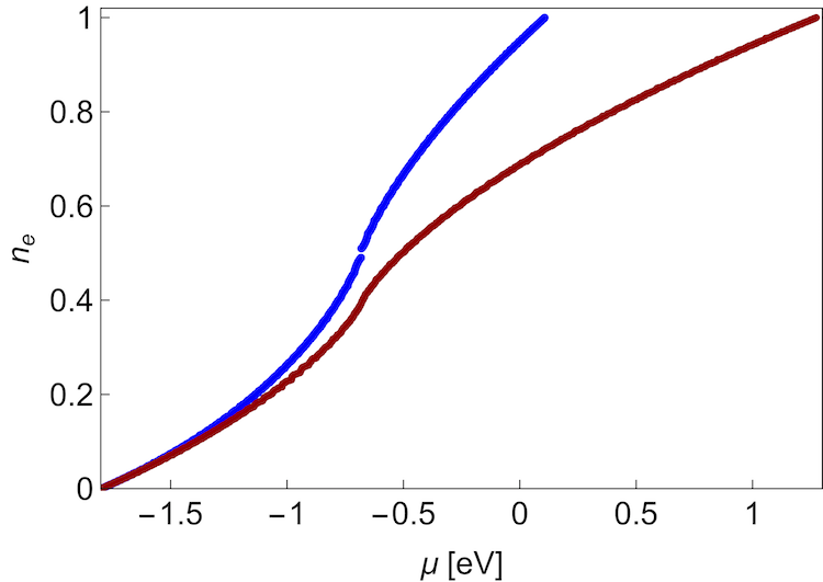
Figure 3: Electron density, $n_{e}$, vs chemical potential, $\mu$, in units of eV, of the upper band of the cuprate lattice, where $V_{dp}=3.45\text{ eV}$ and $t_{pd}=1.13\text{ eV}$. The blue curve corresponds to $t_{pp}=0$, and the red curve corresponds to $t_{pp}=0.8\text{ eV}$. For a given value of $\mu$, we have $n_{e}(t_{pp}\neq 0)\leqslant n_{e}(t_{pp}=0)$.

To formulate the Cooper problem for the upper band, we consider two-particle states with vanishing total momentum. To find the interaction term of the Cooper problem, we use the three sets of creation and annihilation operators $\{\psi_{\mathrm{U},\mathbf{k}\sigma}^{\dagger},\psi_{\mathrm{U},\mathbf{k}\sigma}\}$, $\{\psi_{\mathrm{F},\mathbf{k}\sigma}^{\dagger},\psi_{\mathrm{F},\mathbf{k}\sigma}\}$, and $\{\psi_{\mathrm{L},\mathbf{k}\sigma}^{\dagger},\psi_{\mathrm{L},\mathbf{k}\sigma}\}$, where $\sigma\in\{\uparrow,\downarrow\}$ is a spin index. These operators fulfill the fermionic algebra, and create or annihilate an electron in the the upper-, flat-, and lower band, respectively. In the following we refer to them as band operators. The band operators can be related to the site operators using the components of the eigenvectors of the matrix $\mathrm{h}_{\mathrm{tb}}$; see Appendix C. We assume that the charge-transfer energy, $V_{dp}\equiv V_{d}-V_{p}$, is sufficiently large so that we neglect the interband pairings; cf. Figs. 2(a) and 2(c). We write the interaction Hamiltonian for the Cooper problem as

$$\hat{H}_{\mathrm{int}}= \frac{1}{\mathcal{A}}\sum_{\mathbf{k},\mathbf{k}^{\prime}\in\text{1.BZ}}\mathcal{V}_{\mathbf{k},\mathbf{k}^{\prime}}\psi_{\mathrm{U},\mathbf{k}^{\prime}\downarrow}^{\dagger}\psi_{\mathrm{U},-\mathbf{k}^{\prime}\uparrow}^{\dagger}\psi_{\mathrm{U},-\mathbf{k}\uparrow}\psi_{\mathrm{U},\mathbf{k}\downarrow};$$ (3)

see Appendix C for the derivation. Here, $\mathcal{A}$ denotes the area of the first Brillouin zone and the interaction function $\mathcal{V}_{\mathbf{k},\mathbf{k}^{\prime}}$ is

$$\mathcal{V}_{\mathbf{k},\mathbf{k}^{\prime}}=U_{d}\mathcal{V}_{\mathbf{k},\mathbf{k}^{\prime}}^{(d)}+U_{p}\left(\mathcal{V}_{\mathbf{k},\mathbf{k}^{\prime}}^{(p_{x})}+\mathcal{V}_{\mathbf{k},\mathbf{k}^{\prime}}^{(p_{y})}\right),$$ (4)

where the functions $\mathcal{V}_{\mathbf{k},\mathbf{k}^{\prime}}^{(d)}$, $\mathcal{V}_{\mathbf{k},\mathbf{k}^{\prime}}^{(p_{x})}$, and $\mathcal{V}_{\mathbf{k},\mathbf{k}^{\prime}}^{(p_{y})}$ are derived in Appendix C. The on-site Coulomb interaction strength for $d_{x^{2}-y^{2}}$ orbitals is $U_{d}$, and for both $p_{x}$ and $p_{y}$ orbitals it is $U_{p}$.

Next, we define the Fermi sea by introducing a chemical potential, $\mu$. We define the interacting Fermi sea, $\mathrm{FS_{\mathrm{int}}}$, which includes corrections due to the interaction:

$$\mathrm{FS_{\mathrm{int}}=}\Bigl{\{}\mathbf{k}\in\text{1.BZ}:2E_{\mathbf{k}}^{(\mathrm{U})}+\frac{1}{\mathcal{A}}\mathcal{V}_{\mathbf{k},\mathbf{k}}<2\mu\Bigr{\}},$$ (5)

where the interaction function $\mathcal{V}_{\mathbf{k},\mathbf{k}}$ is obtained as Eq. (4) for $\mathbf{k}^{\prime}=\mathbf{k}$; see Fig. 4. We assume these states to be occupied with an inert Fermi sea. The unoccupied states that are considered in the Cooper problem are the Brillouin zone without the Fermi sea; i.e., $\mathbf{k}\in\text{\text{1.BZ}$\setminus\mathrm{FS_{\mathrm{int}}}$}$. Figures 2(b) and 2(d) show the Fermi surface for $t_{pp}=0$ and $t_{pp}\neq 0$, respectively. The nonvanishing $t_{pp}$ changes the curvature of the dispersive bands, resulting in a Fermi-surface geometry that is in better agreement with the experimental data extracted from ARPES Plakida_HTc_Book ; Leggett_Cuprates ; Alexandrov_Book ; ARPES_1 ; ARPES_2 ; ARPES_3 ; ARPES_4 ; ARPES_5 ; Starfish . Moreover, we vary $\mu$ and calculate the corresponding electron density, $n_{e}$, for both $t_{pp}=0$ and $t_{pp}\neq 0$, resulting in a chemical potential dependence of the density shown in Fig. 3. For a given value of $\mu$ we find that $n_{e}(t_{pp}\neq 0)\leqslant n_{e}(t_{pp}=0)$. As a result, while the desired geometry of the Fermi surface is preserved, we can increase the hole doping for $t_{pp}\neq 0$ hole_doping .

Finally, we include the kinetic energy, so that the total Hamiltonian of the Cooper problem is

$$\hat{H}_{\mathrm{tot}}= \mathop{\sum_{\mathbf{k}\in\,\text{1.BZ}\setminus\mathrm{FS_{\mathrm{int}}}}}_{\sigma\in\{\uparrow,\downarrow\}}\xi_{\mathbf{k}}^{(\mathrm{U})}\psi_{\mathrm{U},\mathbf{k}\sigma}^{\dagger}\psi_{\mathrm{U},\mathbf{k}\sigma}+\frac{1}{\mathcal{A}}$$

$$\times\sum_{\mathbf{k},\mathbf{k}^{\prime}\in\,\text{1.BZ}\setminus\mathrm{FS_{\mathrm{int}}}}\mathcal{V}_{\mathbf{k},\mathbf{k}^{\prime}}\psi_{\mathrm{U},\mathbf{k}^{\prime}\downarrow}^{\dagger}\psi_{\mathrm{U},-\mathbf{k}^{\prime}\uparrow}^{\dagger}\psi_{\mathrm{U},-\mathbf{k}\uparrow}\psi_{\mathrm{U},\mathbf{k}\downarrow},$$ (6)

where $\xi_{\mathbf{k}}^{(\mathrm{U})}=E_{\mathbf{k}}^{(\mathrm{U})}-\mu$ and $\mathcal{V}_{\mathbf{k},\mathbf{k}^{\prime}}$ is given by Eq. (4); see Appendix C.

III cooper problem and pairing equation

The original Cooper problem and its solution show that two electrons that are immersed in an inert Fermi sea form a bound state with an orbital s-wave symmetry for an arbitrarily weak attractive interaction Leggett_Cuprates ; Cooper_paper ; Goodstein_1 ; Abrikosov_book_metals ; Tinkham_1 ; Aschcroft_Mermin_1 . The effective attraction models the phonon-mediated interaction that is dominant over the screened Coulomb repulsion. The interaction model that is used for conventional superconductors is a negative coupling constant in momentum space for the relative kinetic energy of the electrons smaller than the Debye energy; cf. e.g., Refs. Cooper_paper ; Tinkham_1 ; Aschcroft_Mermin_1 . Following the standard Cooper problem, we consider a singlet-state Cooper pair as

$$\left|\Phi\right\rangle=\sum_{\bm{\kappa}\in\text{1.BZ}\setminus\mathrm{FS_{int}}}\phi(\bm{\kappa})\psi_{\mathrm{U},\bm{\kappa}\uparrow}^{\dagger}\psi_{\mathrm{U},-\bm{\kappa}\downarrow}^{\dagger}\left|\mathrm{FS_{int}}\right\rangle,$$ (7)

where $\phi(\bm{\kappa})$ is the wave function of the Cooper pair in momentum space and $\left|\mathrm{FS_{int}}\right\rangle$ denotes the Fermi-sea state; cf. Eq. (5).

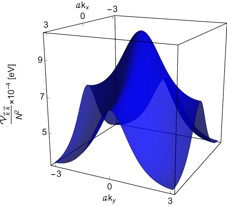
Figure 4: Interaction function $\mathcal{V}_{\mathbf{k},\mathbf{k}}/N^{2}$ in units of eV, cf. Eq. (4), for repulsive on-site interactions, where $N=100$, $V_{dp}=3.45\text{ eV}$, $t_{pd}=1.13\text{ eV}$, $t_{pp}=0.8\text{ eV}$, $U_{d}=10.3\text{ eV}$, and $U_{p}=4.1\text{ eV}.$

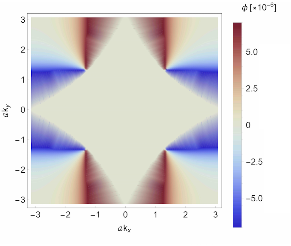
Figure 5: Ground-state wave function, $\phi(ak_{x},ak_{y})$, of a Cooper pair for $N=100$, $V_{dp}=3.45\text{ eV}$, $t_{pd}=1.13\text{ eV}$, $t_{pp}=0.8\text{ eV}$, $U_{d}=10.3\text{ eV}$, $U_{p}=4.1\text{ eV}$, and the hole doing $\delta_{h}\approx 0.104$, where $a$ denotes the lattice constant. The nodal points are visible along the Fermi arcs. The blue color indicates positive values of the wave function, the red color negative ones. The orbital symmetry of the wave function is $d_{x^{2}-y^{2}}$.

To find the ground-state energy and wave function, we consider the eigenvalue problem

$$\hat{H}_{\mathrm{tot}}\left|\Phi\right\rangle=\mathcal{E}\left|\Phi\right\rangle,$$ (8)

where $\mathcal{E}$ is the eigenenergy. We determine the operator $\hat{H}_{\mathrm{tot}}\left|\Phi\right\rangle$ and obtain an eigenequation describing the Cooper pair:

$$\left(\xi_{\mathbf{k}}^{(\mathrm{U})}+\xi_{-\mathbf{k}}^{(\mathrm{U})}+\frac{1}{\mathcal{A}}\mathcal{V}_{\mathbf{k},\mathbf{k}}-\mathcal{E}\right)\phi(\mathbf{k})\qquad\qquad\qquad\qquad$$

$$=-\frac{1}{\mathcal{A}}\mathop{\sum_{\mathbf{k},\mathbf{k}^{\prime}\in\mathrm{1.BZ}\setminus\mathrm{FS_{int}}}}_{\mathbf{k}^{\prime}\neq\mathbf{k}}\mathcal{V}_{\mathbf{k},\mathbf{k}^{\prime}}\phi(\mathbf{k}^{\prime});$$ (9)

see Appendix D. In what fallows we solve Eq. (9) numerically, and determine the ground-state energy, $E_{\text{G}}<0$.

IV ground-state energy and wave function

To solve Eq. (9) numerically, first we discretize the first Brillouin zone as $\mathbf{k}_{j}=(k_{x}^{(j)},k_{y}^{(j)})$, where

$$k_{x}^{(j)},k_{y}^{(j)}=\frac{1}{a}\bigl{[}-\pi+\frac{2\pi}{N}(j-1)\bigr{]}\text{ }\text{ for }j=1,2,\ldots,N.$$ (10)

Here, $a$ denotes the lattice constant and $N\in\mathbb{N}$ is the number of grid points in $x$- and $y$ direction, i.e., $N_{x}=N_{y}=N$. We calculate the electronic band structure numerically and the interaction function $\mathcal{V}_{\mathbf{k},\mathbf{k}^{\prime}}$ at each grid point using Eq. (4). Next, for a given value of $\mu$ we determine the Fermi surface following the relation (5). We note that the number of grid points within the first Brillouin zone is proportional to $N_{x}N_{y}=N^{2}$, so the size of the matrix associated with $\hat{H}_{\mathrm{tot}}$ is proportional to $N^{4}$, cf. Eq. (6). We choose the number of grid points sufficiently large to ensure convergence of the numerical results. We determine the Fermi sea numerically, and exclude it from the first Brillouin zone. We consider $\hat{H}_{\mathrm{tot}}$ on the reduced momentum space that corresponds to the unoccupied states; see Appendix E.

For the regime of attractive interactions, i.e., $U_{d},U_{p}<0$, we find a Cooper pair with an approximate orbital s-wave symmetry; see Appendix F.

For repulsive on-site interactions, $U_{d},U_{p}>0$, the interaction function $\mathcal{V}_{\mathbf{k},\mathbf{k}}$, cf. Eq. (4), has the momentum dependence shown in Fig. 4. The repulsive interaction suppresses the formation of pairs with s-wave symmetry. Instead, the ground state wave function has d-wave symmetry, as shown in Fig. 5, for the lattice parameters $V_{dp}=3.45\text{ eV}$, $t_{pd}=1.13\text{ eV}$, and $t_{pp}=0.8\text{ eV}$ that follow approximately the values given by Ref. Spalek_HTc_Cuprate . The orientation of the maxima and minima, and the location of the nodal points, indicates that the wave function supports an orbital symmetry of $d_{x^{2}-y^{2}}$.

Finally, we vary the hole doping, $\delta_{h}$, by changing the chemical potential, $\mu$ hole_doping . We calculate the corresponding ground-state energy, $E_{\text{G}}$, resulting in Fig. 6. We find that the largest absolute magnitude of the ground-state energy, $|E_{\text{G}}^{(\text{max})}|\sim 0.01\text{ eV}$, occurs near the hole doping $\delta_{h}\sim 0.35$. This converts to a critical temperature of the order of $100\text{ K}$. The behavior of the ground-state energies consistent with Ref. Spalek_HTc_Cuprate qualitatively.

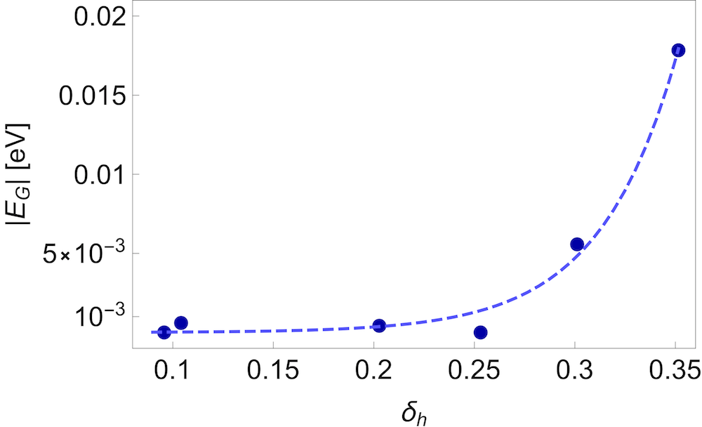
Figure 6: Ground-state energy $|E_{\text{G}}|$ of a Cooper pair in units of eV vs hole doping, $\delta_{h}$ hole_doping , where $N=100$, $V_{dp}=3.45\text{ eV}$, $t_{pd}=1.13\text{ eV}$, $t_{pp}=0.8\text{ eV}$, $U_{d}=10.3\text{ eV}$, and $U_{p}=4.1\text{ eV}$. A largest value of $|E_{\text{G}}|$ corresponding to a critical temperature of the order of 100 K is obtained near the hole doping of 0.35.

V experimental signature in a cold-atom system

We propose to detect the predictions of our analysis in a system of ultracold atoms in an optical lattice. Specifically, we consider fermionic atoms in higher bands of optical lattices. Lattice geometries that resemble the cuprate lattice and related geometries have been realized experimentally for bosonic atoms in Refs. Lieb_optical_1 ; Lieb_optical_2 ; Lieb_optical_3 . Utilizing a Feshbach resonance, the whole range of repulsive interactions is accessible, from weak to strong coupling. In particular, our predictions can be tested quantitatively in the weak-coupling regime.

We propose to use noise correlations of time-of-flight images as an observable to detect the symmetry of the Cooper pair. In the far-field limit, which is achieved for expansions in which the expanded cloud is much larger than the in-situ cloud, the density correlations of the atoms of different spins include the correlations of $\hat{n}(\mathbf{k},\sigma)$ and $\hat{n}(-\mathbf{k},-\sigma)$, where $\hat{n}(\mathbf{k},\sigma)$ is the occupation of the momentum state $\mathbf{k}$ and spin-state $\sigma$ of the in-situ system; see Refs. time_of_flight_1 ; time_of_flight_2 ; noise_correlation_1 ; noise_correlation_2 . This quantity gives access to the square of the pair wave function, depicted in Fig. 5. In particular the angular dependence of its magnitude and the nodal points of the wave function are observable in this quantity.

As a second measurement, we propose to use stirring experiments, as discussed in Ref. noise_correlation_3 . Here, either a focused laser beam is moved through the quantum gas, or a lattice is dragged through it. For fermionic systems, the heating that is induced by this perturbation is suppressed for stirring velocities smaller than the critical velocity $\sim\Delta_{\mathbf{k}_{F}}/|\mathbf{k}_{F}|$. Here, the energy gap $\Delta_{\mathbf{k}_{F}}$ refers to the gap at a momentum $\mathbf{k}_{F}$ that is on the Fermi surface and along the direction of the motion of the stirring potential. Therefore the heating rate and its dependence on the stirring direction maps out the energy gap of the paired state.

VI conclusions

In conclusion, we have presented the solution of the Cooper problem for a cuprate lattice, for repulsive interactions. The band structure of the cuprate lattice consists of three bands, where we focus on densities for which the two lower bands are filled, and the Fermi surface is in the highest band. For these densities, and for repulsive on-site interactions, we demonstrate that the ground state solution of the Cooper problem has a $d_{x^{2}-y^{2}}$ orbital symmetry. The binding energy of the Cooper pair depends strongly on the shape of the Fermi surface. We show that it is small for a connected surface of the shape of a deformed circle, while it is large for surfaces that break up into four disconnected arcs. As a primary, quantitative implementation of our results we propose to create an ultracold Fermi gas in a cuprate lattice. Here, the weak-coupling regime can be implemented naturally due to the tunable nature of these systems, and the dependence on system parameters such as the interaction strength and the Fermi surface geometry mapped out. We pointed out noise correlations and stirring experiments as experimental methods to detect our predictions. As a second platform, we apply our calculation to the three-band model reported for cuprate materials. We emphasize that the interaction strengths of this model suggests that it is in the strongly correlated regime, whereas the Cooper problem is primarily applicable in the weak-coupling limit. However, we present the predictions of the Cooper problem here, given the impact of the Cooper problem on the study of superconductivity, primarily for the purpose of academic completeness. We find that the solution of Cooper problem predicts the experimentally observed $d_{x^{2}-y^{2}}$ symmetry of the electron pairs, a sharp increase of the binding energy with increasing hole doping when the Fermi surface breaks up into four disconnected arcs, and a maximal binding energy of approximately 100 K. This study and its experimental implementation provides a direct analogy between cold-atom systems and the three-band model that is utilized in cuprate materials, and therefore advances the exchange between cold-atom and condensed-matter systems.

ACKNOWLEDGMENTS

This work was funded by the Deutsche Forschungsgemeinschaft (DFG, German Research Foundation) – SFB-925 – project 170620586, and by the Cluster of Excellence ‘Advanced Imaging of Matter’ of the Deutsche Forschungsgemeinschaft (DFG) EXC 2056 - project ID 390715994.

appendix a. derivation of the tight-binding hamiltonian (1)

We consider the cuprate lattice, see Fig. 1, and write the spinless tight-binding Hamiltonian in terms of the site operators in real space:

$$\hat{H}_{\mathrm{tb}}= \sum_{nm}\Bigl{[}V_{d}a_{nm}^{\dagger}a_{nm}+V_{p}b_{nm}^{\dagger}b_{nm}+V_{d}c_{nm}^{\dagger}c_{nm}$$

$$\quad+t_{pd}a_{nm}^{\dagger}b_{nm}+t_{pd}b_{nm}^{\dagger}a_{nm}-t_{pd}a_{nm}^{\dagger}c_{nm}$$

$$\quad-t_{pd}c_{nm}^{\dagger}a_{nm}-t_{pd}a_{nm}^{\dagger}b_{n-1,m}-t_{pd}b_{n-1,m}^{\dagger}a_{nm}$$

$$\quad+t_{pd}a_{nm}^{\dagger}c_{n,m-1}+t_{pd}c_{n,m-1}^{\dagger}a_{nm}-t_{pp}b_{nm}^{\dagger}c_{nm}$$

$$\quad-t_{pp}c_{nm}^{\dagger}b_{nm}+t_{pp}c_{nm}^{\dagger}b_{n-1,m}+t_{pp}b_{n-1,m}^{\dagger}c_{nm}$$

$$\quad-t_{pp}b_{n-1,m}^{\dagger}c_{n,m-1}-t_{pp}c_{n,m-1}^{\dagger}b_{n-1,m}$$

$$\quad+t_{pp}b_{n,m}^{\dagger}c_{n,m-1}+t_{pp}c_{n,m-1}^{\dagger}b_{n,m}\Bigr{]},$$ (A1)

where $n$ and $m$ are two indices for the $x$- and $y$ direction, respectively. Next, we take the Fourier transform of each operator, and obtain the tight-binding Hamiltonian in momentum space:

$$\hat{H}_{\mathrm{tb}}= \sum_{\mathbf{k}\in\,1.\mathrm{BZ}}\Bigl{[}V_{d}a_{\mathbf{k}}^{\dagger}a_{\mathbf{k}}+V_{p}b_{\mathbf{k}}^{\dagger}b_{\mathbf{k}}+V_{d}c_{\mathbf{k}}^{\dagger}c_{\mathbf{k}}$$

$$\quad\quad+t_{pd}a_{\mathbf{k}}^{\dagger}b_{\mathbf{k}}+t_{pd}b_{\mathbf{k}}^{\dagger}a_{\mathbf{k}}-t_{pd}a_{\mathbf{k}}^{\dagger}c_{\mathbf{k}}$$

$$\quad\quad-t_{pd}c_{\mathbf{k}}^{\dagger}a_{\mathbf{k}}-t_{pd}e^{-ik_{x}}a_{\mathbf{k}}^{\dagger}b_{\mathbf{k}}-t_{pd}e^{ik_{x}}b_{\mathbf{k}}^{\dagger}a_{\mathbf{k}}$$

$$\quad\quad+t_{pd}e^{-ik_{y}}a_{\mathbf{k}}^{\dagger}c_{\mathbf{k}}+t_{pd}e^{ik_{y}}c_{\mathbf{k}}^{\dagger}a_{\mathbf{k}}$$

$$\quad\quad-t_{pp}\left(1-e^{ik_{x}}+e^{ik_{x}}e^{-ik_{y}}-e^{-ik_{y}}\right)b_{\mathbf{k}}^{\dagger}c_{\mathbf{k}}$$

$$\quad\quad-t_{pp}\left(1-e^{-ik_{x}}+e^{-ik_{x}}e^{ik_{y}}-e^{ik_{y}}\right)c_{\mathbf{k}}^{\dagger}b_{\mathbf{k}}\Bigr{]}.$$ (A2)

Finally, we define $f(k_{x})=t_{pd}(1-e^{-ik_{x}})$, $g(k_{y})=t_{pd}(1-e^{-ik_{y}})$, and $\tau=t_{pp}/t_{pd}^{2}$, and arrive at Eq. (1).

appendix b. analytical description of the band structure of the cuprate lattice

The characteristic equation associated with Eq. (2) reads as

$$s^{3}+c(k_{x},k_{y})s^{2}+d(k_{x},k_{y})s+e(k_{x},k_{y})=0,$$ (B1)

where

$$c(k_{x},k_{y})= -V_{d}-2V_{p},$$ (B2)

$$d(k_{x},k_{y})= -|f(k_{x})|^{2}-|g(k_{y})|^{2}-\tau^{2}|f(k_{x})|^{2}|g(k_{y})|^{2}$$

$$+V_{p}^{2}+2V_{d}V_{p},$$ (B3)

$$e(k_{x},k_{y})= V_{p}|f(k_{x})|^{2}+V_{p}|g(k_{y})|^{2}+\tau(\tau V_{d}-2)$$

$$\times|f(k_{x})|^{2}|g(k_{y})|^{2}-V_{d}V_{p}^{2},$$ (B4)

and $\tau=t_{pp}/t_{pd}^{2}$. Next, we define a variable $S=s-c(k_{x},k_{y})/3$, and rewrite Eq. (B1) as

$$S^{3}+3p(k_{x},k_{y})S+2q(k_{x},k_{y})=0,$$ (B5)

where

$$p(k_{x},k_{y})= \frac{1}{3}d(k_{x},k_{y})-\frac{1}{9}[c(k_{x},k_{y})]^{2},$$ (B6)

$$q(k_{x},k_{y})= \frac{1}{27}[c(k_{x},k_{y})]^{3}-\frac{1}{6}c(k_{x},k_{y})d(k_{x},k_{y})$$

$$+\frac{1}{2}e(k_{x},k_{y}).$$ (B7)

Following the mathematical formalism represented in Ref. cubic_eq , we calculate the three roots of Eq. (B1), revealing the band structure of the cuprate lattice:

$$E_{\mathbf{k}}^{(\mathrm{U})}= 2\sqrt{-p(k_{x},k_{y})}\cos\left(\frac{\theta(k_{x},k_{y})}{3}\right)-\frac{c(k_{x},k_{y})}{3},$$ (B8)

$$E_{\mathbf{k}}^{(\mathrm{F})}= 2\sqrt{-p(k_{x},k_{y})}\cos\left(\frac{\theta(k_{x},k_{y})+4\pi}{3}\right)-\frac{c(k_{x},k_{y})}{3},$$ (B9)

$$E_{\mathbf{k}}^{(\mathrm{L})}= 2\sqrt{-p(k_{x},k_{y})}\cos\left(\frac{\theta(k_{x},k_{y})+2\pi}{3}\right)-\frac{c(k_{x},k_{y})}{3},$$ (B10)

where $\cos\theta(k_{x},k_{y})=-q(k_{x},k_{y})/\sqrt{-[p(k_{x},k_{y})]^{3}}$; see Fig. 2(c). We note that for $t_{pp}=0$, the three solutions (B8)-(B10) reduce to:

$$\tilde{E}_{\mathbf{k}}^{(\mathrm{U})}= \frac{V_{d}+V_{p}}{2}+2t_{pd}\sqrt{\sin^{2}(\frac{k_{x}}{2})+\sin^{2}(\frac{k_{y}}{2})+\left(\frac{V_{dp}}{4t_{pd}}\right)^{2}},$$ (B11)

$$\tilde{E}_{\mathbf{k}}^{(\mathrm{F})}= V_{p},$$ (B12)

$$\tilde{E}_{\mathbf{k}}^{(\mathrm{L})}= \frac{V_{d}+V_{p}}{2}-2t_{pd}\sqrt{\sin^{2}(\frac{k_{x}}{2})+\sin^{2}(\frac{k_{y}}{2})+\left(\frac{V_{dp}}{4t_{pd}}\right)^{2}},$$ (B13)

respectively; see Fig. 2(a). By comparing Eqs. (B8)-(B13) we find that the next-nearest-neighbor hopping, $t_{pp}$, deforms the flat band $E_{\mathbf{k}}^{(\mathrm{F})}$, and changes the curvature of the dispersive bands $E_{\mathbf{k}}^{(\mathrm{U})}$ and $E_{\mathbf{k}}^{(\mathrm{L})}$.

appendix c. derivation of the hamiltonians (3) and (6)

For the cuprate lattice, see Fig. 1, the interaction Hamiltonian of the Fermi-Hubbard model reads in general as

$$\hat{\tilde{H}}_{\mathrm{int}}= \frac{U_{\mathrm{C}}}{\mathcal{A}}\sum_{\mathbf{k},\mathbf{p},\mathbf{q}\in\,\text{1.BZ}}\alpha_{\mathbf{k}+\mathbf{q},\downarrow}^{\dagger}\alpha_{\mathbf{p}-\mathbf{q},\uparrow}^{\dagger}\alpha_{\mathbf{p},\uparrow}\alpha_{\mathbf{k}\downarrow},$$ (C1)

where $\alpha^{\dagger}\in\{a^{\dagger},b^{\dagger},c^{\dagger}\}$ and $\alpha\in\{a,b,c\}$ denote the creation and annihilation site operators, respectively, $\mathbf{q}$ is the momentum transfer momentum_transfer , and $U_{\mathrm{C}}$ is an on-site Coulomb interaction strength. We notice that for each eigenvalue of $\mathrm{h}_{\mathrm{tb}}$, cf. Eq. (2), there exists a corresponding normalized eigenvector, which we denote as $\mathbf{v}_{\mathbf{k}}^{(\mathrm{U})}=(v_{\mathbf{k}}^{(1;\mathrm{U})},v_{\mathbf{k}}^{(2;\mathrm{U})},v_{\mathbf{k}}^{(3;\mathrm{U})})$, $\mathbf{v}_{\mathbf{k}}^{(\mathrm{F})}=(v_{\mathbf{k}}^{(1;\mathrm{F})},v_{\mathbf{k}}^{(2;\mathrm{F})},v_{\mathbf{k}}^{(3;\mathrm{F})})$, and $\mathbf{v}_{\mathbf{k}}^{(\mathrm{L})}=(v_{\mathbf{k}}^{(1;\mathrm{L})},v_{\mathbf{k}}^{(2;\mathrm{L})},v_{\mathbf{k}}^{(3;\mathrm{L})})$. The index U, F, and L corresponds to the upper-, flat-, and lower band, respectively. The site operators can be related to the band operators using the following relation:

$$\left(\begin{array}[]{c}a_{\mathbf{\mathbf{k}\sigma}}^{\dagger}\\ b_{\mathbf{k}\sigma}^{\dagger}\\ c_{\mathbf{k}\sigma}^{\dagger}\end{array}\right)= \left(\begin{array}[]{ccc}v_{\mathbf{k}}^{(1;\mathrm{U})}&v_{\mathbf{k}}^{(2;\mathrm{U})}&v_{\mathbf{k}}^{(3;\mathrm{U})}\\ v_{\mathbf{k}}^{(1;\mathrm{F})}&v_{\mathbf{k}}^{(2;\mathrm{F})}&v_{\mathbf{k}}^{(3;\mathrm{F})}\\ v_{\mathbf{k}}^{(1;\mathrm{L})}&v_{\mathbf{k}}^{(2;\mathrm{L})}&v_{\mathbf{k}}^{(3;\mathrm{L})}\end{array}\right)^{-1}\left(\begin{array}[]{c}\psi_{\mathrm{U},\mathbf{k}\sigma}^{\dagger}\\ \psi_{\mathrm{F},\mathbf{k}\sigma}^{\dagger}\\ \psi_{\mathrm{L},\mathbf{k}\sigma}^{\dagger}\end{array}\right)$$ (C11)

$$\equiv \left(\begin{array}[]{ccc}v_{11}(\mathbf{k})&v_{12}(\mathbf{k})&v_{13}(\mathbf{k})\\ v_{21}(\mathbf{k})&v_{22}(\mathbf{k})&v_{23}(\mathbf{k})\\ v_{31}(\mathbf{k})&v_{32}(\mathbf{k})&v_{33}(\mathbf{k})\end{array}\right)\left(\begin{array}[]{c}\psi_{\mathrm{U},\mathbf{k}\sigma}^{\dagger}\\ \psi_{\mathrm{F},\mathbf{k}\sigma}^{\dagger}\\ \psi_{\mathrm{L},\mathbf{k}\sigma}^{\dagger}\end{array}\right).$$ (C18)

We can rewrite the interaction Hamiltonian (C1) corresponding to three sites A, B, and C in terms of the band operators using the relation (C18). We recall that here we are primarily interested in a submanifold $\mathcal{S}$, where the total momentum of an electron-pair is vanishing. Because we are interested in the effective Fermi-Hubbard model constituted in the upper band, we prevent the interband pairings as well as the pairings in the flat- and lower band. We write the three interaction Hamiltonians corresponding to $d_{x^{2}-y^{2}},$ $p_{x}$, and $p_{y}$ orbital configurations on the submanifold $\mathcal{S}$ of the upper band in terms of the band operators:

$$\hat{H}_{\mathrm{int}}^{(\Omega)}= \frac{U_{\Omega}}{\mathcal{A}}\sum_{\mathbf{k},\mathbf{k}^{\prime}\in\,\text{1.BZ}}\mathcal{V}_{\mathbf{k},\mathbf{k}^{\prime}}^{(\Omega)}\psi_{\mathrm{U},\mathbf{k}^{\prime}\downarrow}^{\dagger}\psi_{\mathrm{U},-\mathbf{k}^{\prime}\uparrow}^{\dagger}\psi_{\mathrm{U},-\mathbf{k}\uparrow}\psi_{\mathrm{U},\mathbf{k}\downarrow},$$ (C19)

where the label $\Omega$ denotes an orbital configuration which can be $d\equiv d_{x^{2}-y^{2}}$, $p_{x}$, and $p_{y}$. The on-site Coulomb interaction strengths for $d_{x^{2}-y^{2}}$ and $p_{x}$ ($p_{y}$) orbitals are assumed to be $U_{d}$ and $U_{p}$, respectively, and the interaction functions are

$$\mathcal{V}_{\mathbf{k},\mathbf{k}^{\prime}}^{(d)}= v_{11}(\mathbf{k}^{\prime})v_{11}(-\mathbf{k}^{\prime})v_{11}^{*}(-\mathbf{k})v_{11}^{*}(\mathbf{k}),$$ (C20)

$$\mathcal{V}_{\mathbf{k},\mathbf{k}^{\prime}}^{(p_{x})}= v_{21}(\mathbf{k}^{\prime})v_{21}(-\mathbf{k}^{\prime})v_{21}^{*}(-\mathbf{k})v_{21}^{*}(\mathbf{k}),$$ (C21)

$$\mathcal{V}_{\mathbf{k},\mathbf{k}^{\prime}}^{(p_{y})}= v_{31}(\mathbf{k}^{\prime})v_{31}(-\mathbf{k}^{\prime})v_{31}^{*}(-\mathbf{k})v_{31}^{*}(\mathbf{k}).$$ (C22)

The functions $v_{ij}$ have been introduced in Eq. (C18), and $v_{ij}^{*}$ denotes the complex conjugate of $v_{ij}$. The interaction Hamiltonian (3) is obtained as $\hat{H}_{\mathrm{int}}=\hat{H}_{\mathrm{int}}^{(d)}+\hat{H}_{\mathrm{int}}^{(p_{x})}+\hat{H}_{\mathrm{int}}^{(p_{y})}$, where $\mathcal{V}_{\mathbf{k},\mathbf{k}^{\prime}}=\mathcal{V}_{\mathbf{k},\mathbf{k}^{\prime}}^{(d)}+\mathcal{V}_{\mathbf{k},\mathbf{k}^{\prime}}^{(p_{x})}+\mathcal{V}_{\mathbf{k},\mathbf{k}^{\prime}}^{(p_{x})}$ and the Fermi sea has been excluded from the first Brillouin zone.

We note that the tight-binding Hamiltonian (1) in the basis spanned by the band operators is diagonal. For the submanifold $\mathcal{S}$ of the upper band, we find the kinetic energy to be

$$\hat{H}_{\mathrm{kin}}= \mathop{\sum_{\mathbf{k}\in\,\text{1.BZ}}}_{\sigma\in\{\uparrow,\downarrow\}}E_{\mathbf{k}}^{(\mathrm{U})}\psi_{\mathrm{U},\mathbf{k}\sigma}^{\dagger}\psi_{\mathrm{U},\mathbf{k}\sigma},$$ (C23)

where the Fermi sea will be excluded from the first Brillouin zone by introducing a chemical potential, $\mu$. Finally, the total Hamiltonian (6) is obtained as $\hat{H}_{\mathrm{tot}}=\hat{H}_{\mathrm{kin}}+\hat{H}_{\mathrm{int}}$.

appendix d. derivation of the eigenequation (9)

To derive the pairing equation we calculate the resulting operator $\hat{H}_{\mathrm{tot}}\left|\Phi\right\rangle$, where $\hat{H}_{\mathrm{tot}}=\hat{H}_{\mathrm{kin}}+\hat{H}_{\mathrm{int}}$ subject to the interacting Fermi sea. For that, first we apply $\hat{H}_{\mathrm{kin}}$ on $\left|\Phi\right\rangle$. The part corresponding to spin-up, $\hat{H}_{\mathrm{kin}}^{(\uparrow)}$, is obtained to be

$$\hat{H}_{\mathrm{kin}}^{(\uparrow)}\left|\Phi\right\rangle= \sum_{\mathbf{k}\in 1.\mathrm{BZ}\setminus\mathrm{FS_{int}}}\xi_{\mathbf{k}}^{(\mathrm{U})}\psi_{\mathrm{U},\mathbf{k}\uparrow}^{\dagger}\psi_{\mathrm{U},\mathbf{k}\uparrow}\sum_{\bm{\kappa}\in\text{1.BZ}\setminus\mathrm{FS}}\phi(\bm{\kappa})$$

$$\times\psi_{\mathrm{U},\bm{\kappa}\uparrow}^{\dagger}\psi_{\mathrm{U},-\bm{\kappa}\downarrow}^{\dagger}\left|\mathrm{FS_{int}}\right\rangle$$

$$= \sum_{\bm{\kappa}\in 1.\mathrm{BZ}\setminus\mathrm{FS_{int}}}\delta_{\bm{\kappa}\mathbf{k}}\xi_{\mathbf{k}}^{(\mathrm{U})}\left|\Phi\right\rangle,$$ (D1)

where $\delta_{\bm{\kappa}\mathbf{k}}$ denotes the Kronecker delta. To find the effect of the spin-down part, $\hat{H}_{\mathrm{kin}}^{(\downarrow)}$, we define $\bm{\kappa}^{\prime}\equiv-\bm{\kappa}$, and rewrite the singlet-state Cooper pair (7) in terms of $\bm{\kappa}^{\prime}$. We obtain that

$$\hat{H}_{\mathrm{kin}}^{(\downarrow)}\left|\Phi\right\rangle=\sum_{\bm{\kappa}^{\prime}\in 1.\mathrm{BZ}\setminus\mathrm{FS_{int}}}\delta_{\bm{\kappa}^{\prime}\mathbf{k}}\xi_{\bm{\kappa}^{\prime}}^{(\mathrm{U})}\left|\Phi\right\rangle.$$ (D2)

Equations (D1) and (D2) result in:

$$\hat{H}_{\mathrm{kin}}\left|\Phi\right\rangle= \sum_{\mathbf{k}\in\mathrm{1.BZ}\setminus\mathrm{FS_{int}}}\left(\xi_{\mathbf{k}}^{(\mathrm{U})}+\xi_{-\mathbf{k}}^{(\mathrm{U})}\right)\left|\Phi\right\rangle.$$ (D3)

Next, we apply $\hat{H}_{\mathrm{int}}$ on $\left|\Phi\right\rangle$. Here we split up the interaction Hamiltonian to the diagonal and off-diagonal parts. For the diagonal part we obtain:

$$\hat{H}_{\mathrm{int}}^{(\mathrm{diag})}\left|\Phi\right\rangle= \frac{1}{\mathcal{A}}\sum_{\mathbf{k}\in 1.\mathrm{BZ}\setminus\mathrm{FS_{int}}}\mathcal{V}_{\mathbf{k},\mathbf{k}}\psi_{\mathrm{U},\mathbf{k}\downarrow}^{\dagger}\psi_{\mathrm{U},-\mathbf{k}\uparrow}^{\dagger}\psi_{\mathrm{U},-\mathbf{k}\uparrow}\psi_{\mathrm{U},\mathbf{k}\downarrow}\sum_{\bm{\kappa}\in 1.\mathrm{BZ}\setminus\mathrm{FS_{int}}}\phi(\bm{\kappa})\psi_{\mathrm{U},\bm{\kappa}\uparrow}^{\dagger}\psi_{\mathrm{U},-\bm{\kappa}\downarrow}^{\dagger}\left|\mathrm{FS_{int}}\right\rangle$$

$$= \frac{1}{\mathcal{A}}\sum_{\mathbf{k}\in 1.\mathrm{BZ}\setminus\mathrm{FS_{int}}}\mathcal{V}_{\mathbf{k},\mathbf{k}}\sum_{\bm{\kappa}\in 1.\mathrm{BZ}\setminus\mathrm{FS_{int}}}\phi(-\mathbf{k})\psi_{\mathrm{U},-\mathbf{k}\uparrow}^{\dagger}\psi_{\mathrm{U},\mathbf{k}\downarrow}^{\dagger}\left|\mathrm{FS_{int}}\right\rangle$$

$$+\frac{1}{\mathcal{A}}\sum_{\mathbf{k}\in 1.\mathrm{BZ}\setminus\mathrm{FS_{int}}}\mathcal{V}_{\mathbf{k},\mathbf{k}}\sum_{\bm{\kappa}\in 1.\mathrm{BZ}\setminus\mathrm{FS_{int}}}\delta_{\mathbf{k},-\bm{\kappa}}\phi(\bm{\kappa})\psi_{\mathrm{U},\mathbf{k}\downarrow}^{\dagger}\psi_{\mathrm{U},-\mathbf{k}\uparrow}\psi_{\mathrm{U},-\mathbf{k}\uparrow}^{\dagger}\psi_{\mathrm{U},\bm{\kappa}\uparrow}^{\dagger}\left|\mathrm{FS_{int}}\right\rangle$$

$$= \frac{1}{\mathcal{A}}\sum_{\mathbf{k}\in 1.\mathrm{BZ}\setminus\mathrm{FS_{int}}}\mathcal{V}_{\mathbf{k},\mathbf{k}}\left|\Phi\right\rangle,$$ (D4)

where $\mathcal{A}$ denotes the area of the first Brillouin zone. For the off-diagonal part we obtain:

$$\hat{H}_{\mathrm{int}}^{(\text{off-diag})}\left|\Phi\right\rangle= \frac{1}{\mathcal{A}}\mathop{\sum_{\mathbf{k},\mathbf{k}^{\prime}\in 1.\mathrm{BZ}\setminus\mathrm{FS_{int}}}}_{\mathbf{k}\neq\mathbf{k}^{\prime}}\mathcal{V}_{\mathbf{k},\mathbf{k}^{\prime}}\psi_{\mathrm{U},\mathbf{k}^{\prime}\downarrow}^{\dagger}\psi_{\mathrm{U},-\mathbf{k}^{\prime}\uparrow}^{\dagger}\sum_{\bm{\kappa}\in 1.\mathrm{BZ}\setminus\mathrm{FS}}\phi(\bm{\kappa})\psi_{\mathrm{U},-\mathbf{k}\uparrow}\psi_{\mathrm{U},\mathbf{k}\downarrow}\psi_{\mathrm{U},\bm{\kappa}\uparrow}^{\dagger}\psi_{\mathrm{U},-\bm{\kappa}\downarrow}^{\dagger}\left|\mathrm{FS_{int}}\right\rangle$$

$$= \frac{-1}{\mathcal{A}}\mathop{\sum_{\mathbf{k},\mathbf{k}^{\prime}\in 1.\mathrm{BZ}\setminus\mathrm{FS_{int}}}}_{\mathbf{k}\neq\mathbf{k}^{\prime}}\mathcal{V}_{\mathbf{k},\mathbf{k}^{\prime}}\psi_{\mathrm{U},\mathbf{k}^{\prime}\downarrow}^{\dagger}\psi_{\mathrm{U},-\mathbf{k}^{\prime}\uparrow}^{\dagger}\sum_{\mathbf{k}^{\prime}\in 1.\mathrm{BZ}\setminus\mathrm{FS_{int}}}\phi(\mathbf{k}^{\prime})\left(\hat{1}-\psi_{\mathrm{U},\mathbf{k}^{\prime}\uparrow}^{\dagger}\psi_{\mathrm{U},\mathbf{k}^{\prime}\uparrow}\right)\left|\mathrm{FS_{int}}\right\rangle$$

$$= \frac{1}{\mathcal{A}}\mathop{\sum_{\mathbf{k},\mathbf{k}^{\prime}\in 1.\mathrm{BZ}\setminus\mathrm{FS_{int}}}}_{\mathbf{k}\neq\mathbf{k}^{\prime}}\mathcal{V}_{\mathbf{k},\mathbf{k}^{\prime}}\left|\Phi\right\rangle.$$ (D5)

Equations (D4) and (D5) result in

$$\hat{H}_{\mathrm{int}}\left|\Phi\right\rangle= \frac{1}{\mathcal{A}}\sum_{\mathbf{k},\mathbf{k}^{\prime}\in 1.\mathrm{BZ}\setminus\mathrm{FS_{int}}}\mathcal{V}_{\mathbf{k},\mathbf{k}^{\prime}}\left|\Phi\right\rangle.$$ (D6)

Finally, we insert Eqs. (D3) and (D6) into the eigenvalue problem (8), and arrive at the pairing equation (9).

appendix e. numerical calculation of eq. (9)

As discussed in the text, to solve Eq. (9) numerically we discretize the first Brillouin zone equidistantly following the relation (10). In order to increase the number of the grid points in each direction and to achieve the numerical stability, first we calculate the interacting Fermi surface using the relation

$$\mathrm{FS_{\mathrm{int}}=}\Bigl{\{}\mathbf{k}^{(j)}\in\text{1.BZ}:2E_{\mathbf{k}^{(j)}}^{(\mathrm{U})}+\frac{1}{N^{2}}\mathcal{V}_{\mathbf{k}^{(j)},\mathbf{k}^{(j)}}<2\mu\Bigr{\}},$$ (E1)

and exclude it from the first Brillouin zone. Next, we constitute the pairing equation (9) on the reduced momentum space as

$$\left(\xi_{\mathbf{k}_{j}}^{(\mathrm{U})}+\xi_{-\mathbf{k}_{j}}^{(\mathrm{U})}+\frac{1}{N^{2}}\mathcal{V}_{\mathbf{k}_{j},\mathbf{k}_{j}}\right)\phi(\mathbf{k}_{j})$$

$$+\frac{1}{N^{2}}\mathop{\sum_{\mathbf{k}_{j},\mathbf{k}^{\prime}_{j}\in\mathrm{1.BZ}\setminus\mathrm{FS_{int}}}}_{\mathbf{k}^{\prime}_{j}\neq\mathbf{k}_{j}}\mathcal{V}_{\mathbf{k}_{j},\mathbf{k}_{j}^{\prime}}\phi(\mathbf{k}^{\prime}_{j}) =\mathcal{E}_{j}\phi(\mathbf{k}_{j}),$$ (E2)

for $j=1,2,\ldots,N$. Finally, we diagonalize Eq. (E2), and obtain the eigenenergies $\mathcal{E}_{j}$. Among $\mathcal{E}_{j}$, the desired ground-state energy, $E_{\text{G}},$ is the one which is negative and has the largest absolute value.

Finally, we notice that the behavior of the desired eigenvalues as a function of the chemical potential, $\mu$, might display a zigzag effect due to the finite discretization of the momentum space. To prevent this behavior, for the noninteracting regime, we calculate the smallest value of the eigenenergy, $E_{0}$, of Eq. (E2) for the occupied states. Next, for the interacting regime, we add $E_{0}$ within the first bracket of Eq. (E2), and calculate the ground-state energy for the unoccupied states.

appendix f. ground-state solution for the attractive regime

As expected, for the attractive regime, $U_{d},U_{p}<0$, the ground-state solution supports an orbital s-wave symmetry. Figure 7 shows the wave function for $U_{d}=-2\text{ eV}$ and $U_{p}=-1\text{ eV}.$

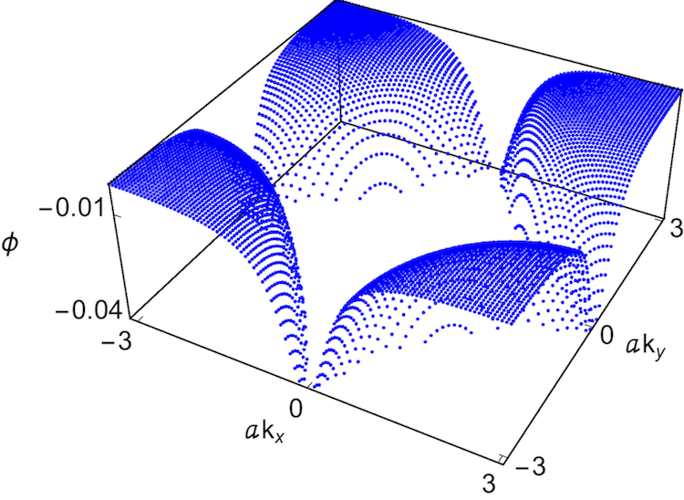
Figure 7: Ground-state wave function of the Cooper pair in the attractive regime of the Fermi-Hubbard model (6), where $N=100$, $V_{dp}=3.45\text{ eV}$, $t_{pd}=1.13\text{ eV}$, $t_{pp}=0.8\text{ eV}$, $\mu\approx-0.679\text{ eV}$, $U_{d}=-2\text{ eV}$, and $U_{p}=-1\text{ eV}$. The wave function supports an orbital s-wave symmetry.

References

- (1) E. H. Lieb, Phys. Rev. Lett. 62, 1201 (1989).
- (2) M. Niţǎ, B. Ostahie, and A. Aldea, Phys. Rev. B 87, 125428 (2013).
- (3) N. Plakida, High-Temperature Cuprate Superconductors: Experiment, Theory, and Applications (Springer, Berlin, 2010), Chaps. 2 and 3.
- (4) A. J. Leggett, Quantum Liquids (Oxford University Press, New York, 2006), Chaps. 5 and 7.
- (5) C. J. Pethick and H. Smith, Bose–Einstein Condensation in Dilute Gases (Cambridge University Press, New York, 2008), Chap. 5.
- (6) J. Fortágh and C. Zimmermann, Rev. Mod. Phys. 79, 235 (2007).
- (7) R. Shen, L. B. Shao, B. Wang, and D. Y. Xing, Phys. Rev. B 81, 041410(R) (2010).
- (8) V. Apaja, M. Hyrkäs, and M. Manninen, Phys. Rev. A 82, 041402(R) (2010).
- (9) S. Taie, H. Ozawa, T. Ichinose, T. Nishio, S. Nakajima, and Y. Takahashi, Sci. Adv. 1, e1500854 (2015).
- (10) M. R. Slot, T. S. Gardenier, P. H. Jacobse, G. C. P. van Miert, S. N. Kempkes, S. J. M. Zevenhuizen, C. M. Smith, D. Vanmaekelbergh, and I. Swart, Nat. Phys. 13, 672 (2017).
- (11) R. Drost, T. Ojanen, A. Harju, and P. Liljeroth, Nat. Phys. 13, 668 (2017).
- (12) S. Mukherjee, A. Spracklen, D. Choudhury, N. Goldman, P. Öhberg, E. Andersson, and R. R. Thomson, Phys. Rev. Lett. 114, 245504 (2015).
- (13) W. Jiang, H. Huang, and F. Liu, Nat. Comm. 10, 2207 (2019).
- (14) B. Cui, X. Zheng, J. Wang, D. Liu, S. Xie, and B. Huang, Nat. Comm. 11, 66 (2020).
- (15) J. D. Bodyfelt, D. Leykam, C. Danieli, X. Yu, and S. Flach, Phys. Rev. Lett. 113, 236403 (2014).
- (16) D. Leykam, A. Andreanov, and S. Flach, Adv. Phys. X 3, 1473052 (2018).
- (17) N. B. Kopnin, T. T. Heikkilä, and G. E. Volovik, Phys. Rev. B 83, 220503(R) (2011).
- (18) V. I. Iglovikov, F. Hébert, B. Grémaud, G. G. Batrouni, and R. T. Scalettar, Phys. Rev. B 90, 094506 (2014).
- (19) S. Peotta and P. Törmä, Nat. Comm. 6, 8944 (2014).
- (20) A. Julku, S. Peotta, T. I. Vanhala, D. -H. Kim, and P. Törmä, Phys. Rev. Lett. 117, 045303 (2016).
- (21) K. Kobayashi, M. Okumura, S. Yamada, M. Machida, and H. Aoki, Phys. Rev. B 94, 214501 (2016).
- (22) M. Tovmasyan, S. Peotta, P. Törmä, and S. D. Huber, Phys. Rev. B 94, 245149 (2016).
- (23) J. R. Schrieffer and J. S. Brooks (eds.), Handbook of High-Temperature Superconductivity: Theory and Experiment (Springer, New York, 2007), Chap. 1.
- (24) J. W. Lynn (ed.), High-Temperature Superconductivity (Springer, New York, 1990), Chap. 5.
- (25) P. W. Anderson, The Theory of Superconductivity in the High- Cuprates (Princeton University Press, Princeton, New Hersey, 1997), Chap. 1.
- (26) S. Uchida, High Temperature Superconductivity: The Road to Higher Critical Temperature (Springer, Tokyo, 2015), Chap. 3.
- (27) A. A. Abrikosov, Int. J. Mod. Phys. 13, 3405 (1999).
- (28) S. R. Park, D. J. Song, C. S. Leem, C. Kim, C. Kim, B. J. Kim, and H. Eisaki, Phys. Rev. Lett. 101, 117006 (2008).
- (29) S. Johnston, F. Vernay, B. Moritz, Z. -X. Shen, N. Nagaosa, J. Zaanen, and T. P. Devereaux, Phys. Rev. B 82, 064513 (2010).
- (30) P. J. Carbotte, T. Timusk, and J. Hwang, Rep. Prog. Phys. 74, 066501 (2011).
- (31) A. S. Alexandrov, J. H. Samson, and G. Sica, Europhys. Lett. 100, 17011 (2012).
- (32) P. Monthoux, A. V. Balatsky, and D. Pines, Phys. Rev. Lett. 67, 3448 (1991).
- (33) V. M. Krasnov, S. -O. Katterwe, and A. Rydh, Nat. Comm. 4, 2970 (2013).
- (34) H. Rietschel and L. J. Sham, Phys. Rev. B 28, 5100 (1983).
- (35) A. Bill, H. Morawitz, and V. Z. Kresin, Phys. Rev. B 68, 144519 (2003).
- (36) G. S. Atwal and N. W. Ashcroft, Phys. Rev. B 70, 104513 (2004).
- (37) E. A. Pashitskii and V. I. Pentegov, Low Temp. Phys. 34, 113 (2008).
- (38) A. S. Alexandrov and V. V. Kabanov, Phys. Rev. Lett. 106, 136403 (2011).
- (39) A. S. Alexandrov, Strong-Coupling Theory of High-Temperature Superconductivity (Cambridge University Press, Cambridge, 2013), Chaps. 6 and 8.
- (40) A. Damascelli, Z. Hussain, and Z. -X. Shen, Rev. Mod. Phys. 75, 473 (2003).
- (41) D. Koralek, J. F. Douglas, N. C. Plumb, Z. Sun, A. V. Fedorov, M. M. Murnane, H. C. Kapteyn, S. T. Cundiff, Y. Aiura, K. Oka, H. Eisaki, and D. S. Dessau, Phys. Rev. Lett. 96, 017005 (2006).
- (42) J. D. Koralek, J. F. Douglas, N. C. Plumb, J. D. Griffith, S. T. Cundiff, H. C. Kapeteyn, M. M. Murnane, and D. S. Dessau, Rev. Sci. Instrum. 78, 053905 (2007).
- (43) G. Liu, G. Wang, Y. Zhu, H. Zhang, G. Zhang, X. Wang, Y. Zhou, W. Zhang, H. Liu, L. Zhao, J. Meng, X. Dong, C. Chen, Z. Xu, and X. J. Zhou, Rev. Sci. Instrum. 79, 023105 (2008).
- (44) H. Li, X. Zhou, S. Parham, T. J. Reber, H. Berger, G. B. Arnold, and D. S. Dessau, Nat. Comm. 9, 26 (2018).
- (45) H. Li, X. Zhou, S. Parham, K. N. Gordon, R. D. Zhong, J. Schneeloch, G. D. Gu, Y. Huang, H. Berger, G. B. Arnold, and D. S. Dessau, arXiv:1809.02194v2.
- (46) M. Zegrodnik, A. Biborski, M. Fidrysiak, and J. Spałek, Phys. Rev. B 99, 104511 (2019).
- (47) J. Kaczmarczyk, J. Bünemann, and J. Spałek, New J. Phys. 16, 073018 (2014).
- (48) J. Spałek, M. Zegrodnik, and J. Kaczmarczyk, Phys. Rev. B 95, 024506 (2017).
- (49) P. W. Phillips, L. Yeo, and E. W. Huang, Nat. Phys. 16, 1175 (2020).
- (50) G. Knizia and G. K. -L. Chan, Phys. Rev. Lett. 109, 186404 (2012).
- (51) T. I. Vanhala and P. Törmä, Phys. Rev. B 97, 075112 (2018).
- (52) S. Zhang, J. Carlson, and J. E. Gubernatis, Phys. Rev. Lett. 74, 3652 (1995).
- (53) J. Jordan, R. Orús, G. Vidal, F. Verstraete, and J. I. Cirac, Phys. Rev. Lett. 101, 250602 (2008).
- (54) E. M. Stoudenmire and S. R. White, Annu. Rev. Condens. Matter Phys. 3, 111 (2012).
- (55) M. Kitatani, N. Tsuji, and H. Aoki, Phys. Rev. B 95, 075109 (2017).
- (56) L. N. Cooper, Phys. Rev. 104, 1189 (1956).
- (57) D. L. Goodstein, States of Matter (Dover, New York, 1985), Chap. 5.
- (58) A. A. Abrikosov, Fundamentals of the Theory of Metals (Dover, New York, 2017), Chap. 16.
- (59) M. Tinkham, Introduction to Superconductivity (Dover, New York, 2004), Chap. 3.
- (60) N. W. Ashcroft and N. D. Mermin, Solid State Physics (Brooks/Cole, Belmont, CA, 1976), Chaps. 26 and 34.
- (61) A. Sanayei, P. Naidon, and L. Mathey Phys. Rev. Research 2, 013341 (2020).
- (62) A. Sanayei and L. Mathey, arXiv:2007.13511.
- (63) To define the hole doping, , here we follow this convention: At the half-filling the electron density , and the hole doping is vanishing, . As we decrease , we inject more holes into the desired momentum space, which increases . Here the hole doping is obtained as , for .
- (64) M. Lewenstein, A. Sanpera, and V. Ahufinger, Ultracold Atoms in Optical Lattices: Simulating Quantum Many-Body Systems (Oxford University Press, 2012), Chap. 14.
- (65) M. Inguscio and L. Fallani, Atomic Physics: Precise Measurements & Ultracold Matter (Oxford University Press, Oxford, 2013), Chap. 6.
- (66) E. Altman, E. Demler, and M. D. Lukin , Phys. Rev. A 70, 013603 (2004).
- (67) L. Mathey, A. Vishwanath, and E. Altman, Phys. Rev. A 79, 013609 (2009).
- (68) V. Pal Singh, W. Weimer, K. Morgener, J. Siegl, K. Hueck, N. Luick, H. Moritz, and L. Mathey Phys. Rev. A 93, 023634 (2016).
- (69) I. J. Zucker, Math. Gazet. 92, 264 (2008).
- (70) By “momentum transfer” we mean the difference of the in-state and out-state momenta of a particle; see, e.g., J. R. Taylor, Scattering Theory: The Quantum Theory of Nonrelativistic Collisions (Dover, New York, 2006).