On Margin Maximization in Linear and ReLU Networks

Abstract

The implicit bias of neural networks has been extensively studied in recent years. Lyu and Li (2019) showed that in homogeneous networks trained with the exponential or the logistic loss, gradient flow converges to a KKT point of the max margin problem in parameter space. However, that leaves open the question of whether this point will generally be an actual optimum of the max margin problem. In this paper, we study this question in detail, for several neural network architectures involving linear and ReLU activations. Perhaps surprisingly, we show that in many cases, the KKT point is not even a local optimum of the max margin problem. On the flip side, we identify multiple settings where a local or global optimum can be guaranteed.

1 Introduction

A central question in the theory of deep learning is how neural networks generalize even when trained without any explicit regularization, and when there are far more learnable parameters than training examples. In such optimization problems there are many solutions that label the training data correctly, and gradient descent seems to prefer solutions that generalize well (Zhang et al., 2016). Hence, it is believed that gradient descent induces an implicit bias (Neyshabur et al., 2014, 2017), and characterizing this bias has been a subject of extensive research in recent years.

A main focus in the theoretical study of implicit bias is on homogeneous neural networks. These are networks where scaling the parameters by any factor $\alpha>0$ scales the predictions by $\alpha^{L}$ for some constant $L$. For example, fully-connected and convolutional ReLU networks without bias terms are homogeneous. Lyu and Li (2019) proved that in linear and ReLU homogeneous networks trained with the exponential or the logistic loss, if gradient flow converges to a sufficiently small loss, then the direction to which the parameters of the network converge can be characterized as a first order stationary point (KKT point) of the maximum margin problem in parameter space. Namely, the problem of minimizing the $\ell_{2}$ norm of the parameters under the constraints that each training example is classified correctly with margin at least $1$. They also showed that this KKT point satisfies necessary conditions for optimality. However, the conditions are not known to be sufficient even for local optimality. It is analogous to showing that some unconstrained optimization problem converges to a point with gradient zero, without proving that it is either a global or a local minimum. Thus, the question of when gradient flow maximizes the margin remains open. Understanding margin maximization may be crucial for explaining generalization in deep learning, and it might allow us to utilize margin-based generalization bounds for neural networks.

In this work we consider several architectures of homogeneous neural networks with linear and ReLU activations, and study whether the aforementioned KKT point is guaranteed to be a global optimum of the maximum margin problem, a local optimum, or neither. Perhaps surprisingly, our results imply that in many cases, such as depth-$2$ fully-connected ReLU networks and depth-$2$ diagonal linear networks, the KKT point may not even be a local optimum of the maximum-margin problem. On the flip side, we identify multiple settings where a local or global optimum can be guaranteed.

We now describe our results in a bit more detail. We denote by ${\cal N}$ the class of neural networks without bias terms, where the weights in each layer might have an arbitrary sparsity pattern, and weights might be shared. The class ${\cal N}$ contains, for example, convolutional networks. Moreover, we denote by ${\cal N}_{\text{no-share}}$ the subclass of ${\cal N}$ that contains only networks without shared weights, such as fully-connected networks and diagonal networks (cf. Gunasekar et al. (2018b); Yun et al. (2020)). We describe our main results below, and also summarize them in Tables 1 and 2.

Fully-connected networks:

• In linear fully-connected networks of any depth the KKT point is a global optimum.

• In fully-connected depth-$2$ ReLU networks the KKT point may not even be a local optimum. Moreover, this negative result holds with constant probability over the initialization, i.e., there is a training dataset such that gradient flow with random initialization converges with positive probability to the direction of a KKT point which is not a local optimum.

Depth-$2$ networks in ${\cal N}$:

• In linear networks with sparse weights, and specifically in diagonal networks, we show that the KKT point may not be a local optimum.

• In our proof of the above negative result, the KKT point contains a neuron whose weights vector is zero. However, in practice gradient descent often converges to networks that do not contain such zero neurons. We show that for linear networks in ${\cal N}_{\text{no-share}}$, if the KKT point has only non-zero weights vectors, then it is a global optimum. Thus, despite the above negative result, a reasonable assumption on the KKT point allows us to obtain a strong positive result. We also show some implications of our results on margin maximization in predictor space for depth-$2$ diagonal linear networks (see Remark 4.1).

• For ReLU networks in ${\cal N}_{\text{no-share}}$, in order to obtain a positive result we need a stronger assumption. We show that if the KKT point is such that for every input in the dataset the input to every hidden neuron in the network is non-zero, then it is guaranteed to be a local optimum (but not necessarily a global optimum).

• We prove that assuming the network does not have shared weights is indeed required in the above positive results, since for networks with shared weights (such as convolutional networks) they no longer hold.

Deep networks in ${\cal N}$:

• We discuss the difficulty in extending our positive results to deeper networks. Then, we study a weaker notion of margin maximization: maximizing the margin for each layer separately. For linear networks of depth $m\geq 2$ in ${\cal N}$ (including networks with shared weights), we show that the KKT point is a global optimum of the per-layer maximum margin problem. For ReLU networks the KKT point may not even be a local optimum of this problem, but under the assumption on non-zero inputs to all neurons it is a local optimum.

As detailed above, we consider several different settings, and the results vary dramatically between the settings. Thus, our results draw a somewhat complicated picture. Overall, our negative results show that even in very simple settings gradient flow does not maximize the margin even locally, and we believe that these results should be used as a starting point for studying which assumptions are required for proving margin maximization. Our positive results indeed show that under certain reasonable assumptions gradient flow maximizes the margin (either locally or globally). Also, the notion of per-layer margin maximization which we consider suggests another path for obtaining positive results on the implicit bias.

In the paper, our focus is on understanding what can be guaranteed for the KKT convergence points specified in Lyu and Li (2019). Accordingly, in most of our negative results, the construction assumes some specific initialization of gradient flow, and does not quantify how “likely” they are to be reached under some random initialization. An exception is our negative result for depth-$2$ fully-connected ReLU networks (Theorem 3.2), which holds with constant probability under reasonable random initializations. Understanding whether this can be extended to the other settings we consider is an interesting problem for future research.

Our paper is structured as follows: In Section 2 we provide necessary notations and definitions, and discuss relevant prior results. Additional related works are discussed in Appendix A. In Sections 3, 4 and 5 we state our results on fully-connected networks, depth-$2$ networks in ${\cal N}$ and deep networks in ${\cal N}$ respectively, and provide some proof ideas. All formal proofs are deferred to Appendix C.

	Linear	ReLU
Fully-connected	Global (Thm. 3.1)	Not local  (Thm. 3.2)
${\cal N}_{\text{no-share}}$	Not local  (Thm. 4.1)	Not local  (Thm. 3.2)
${\cal N}_{\text{no-share}}$ assuming non-zero weights vectors	Global  (Thm. 4.2)	Not local  (Thm. 4.2)
${\cal N}_{\text{no-share}}$ assuming non-zero inputs to all neurons	Global (Thm. 4.2)	Local,    Not global  (Thm. 4.3)
${\cal N}$ assuming non-zero inputs to all neurons	Not local  (Thm. 4.4)	Not local  (Thm. 4.4)

Table 1: Results on depth-$2$ networks.

	Linear	ReLU
Fully-connected	Global (Thm. 3.1)	Not local  (Thm. 3.2)
${\cal N}_{\text{no-share}}$ assuming non-zero inputs to all neurons	Not local  (Thm. 5.1)	Not local  (Thm. 5.1)
${\cal N}$ - max margin for each layer separately	Global (Thm. 5.2)	Not local  (Thm. 5.3)
${\cal N}$ - max margin for each layer separately, assuming non-zero inputs to all neurons	Global (Thm. 5.2)	Local,    Not global  (Thm. 5.4)

Table 2: Results on deep networks.

2 Preliminaries

Notations.

We use bold-faced letters to denote vectors, e.g., $\mathbf{x}=(x_{1},\ldots,x_{d})$. For $\mathbf{x}\in{\mathbb{R}}^{d}$ we denote by $\left\|\mathbf{x}\right\|$ the Euclidean norm. We denote by $\mathds{1}(\cdot)$ the indicator function, for example $\mathds{1}(t\geq 5)$ equals $1$ if $t\geq 5$ and $0$ otherwise. For an integer $d\geq 1$ we denote $[d]=\{1,\ldots,d\}$.

Neural networks.

A fully-connected neural network $\Phi$ of depth $m\geq 2$ is parameterized by a collection ${\boldsymbol{\theta}}=[W^{(l)}]_{l=1}^{m}$ of weight matrices, such that for every layer $l\in[m]$ we have $W^{(l)}\in{\mathbb{R}}^{d_{l}\times d_{l-1}}$. Thus, $d_{l}$ denotes the number of neurons in the $l$-th layer (i.e., the width of the layer). We assume that $d_{m}=1$ and denote by $d:=d_{0}$ the input dimension. The neurons in layers $[m-1]$ are called hidden neurons. A fully-connected network computes a function $\Phi({\boldsymbol{\theta}};\cdot):{\mathbb{R}}^{d}\to{\mathbb{R}}$ defined recursively as follows. For an input $\mathbf{x}\in{\mathbb{R}}^{d}$ we set $\mathbf{h}^{\prime}_{0}=\mathbf{x}$, and define for every $j\in[m-1]$ the input to the $j$-th layer as $\mathbf{h}_{j}=W^{(j)}\mathbf{h}^{\prime}_{j-1}$, and the output of the $j$-th layer as $\mathbf{h}^{\prime}_{j}=\sigma(\mathbf{h}_{j})$, where $\sigma:{\mathbb{R}}\to{\mathbb{R}}$ is an activation function that acts coordinate-wise on vectors. Then, we define $\Phi({\boldsymbol{\theta}};\mathbf{x})=W^{(m)}\mathbf{h}^{\prime}_{m-1}$. Thus, there is no activation function in the output neuron. When considering depth-$2$ fully-connected networks we often use a parameterization ${\boldsymbol{\theta}}=[\mathbf{w}_{1},\ldots,\mathbf{w}_{k},\mathbf{v}]$ where $\mathbf{w}_{1},\ldots,\mathbf{w}_{k}$ are the weights vectors of the $k$ hidden neurons (i.e., correspond to the rows of the first layer’s weight matrix) and $\mathbf{v}$ are the weights of the second layer.

We also consider neural networks where some weights can be missing or shared. We define a class ${\cal N}$ of networks that may contain sparse and shared weights as follows. A network $\Phi$ in ${\cal N}$ is parameterized by ${\boldsymbol{\theta}}=[\mathbf{u}^{(l)}]_{l=1}^{m}$ where $m$ is the depth of $\Phi$, and $\mathbf{u}^{(l)}\in{\mathbb{R}}^{p_{l}}$ are the parameters of the $l$-th layer. We denote by $W^{(l)}\in{\mathbb{R}}^{d_{l}\times d_{l-1}}$ the weight matrix of the $l$-th layer. The matrix $W^{(l)}$ is described by the vector $\mathbf{u}^{(l)}$, and a function $g_{l}:[d_{l}]\times[d_{l-1}]\to[p_{l}]\cup\{0\}$ as follows: $W^{(l)}_{ij}=0$ if $g_{l}(i,j)=0$, and $W^{(l)}_{ij}=u_{k}$ if $g_{l}(i,j)=k>0$. Thus, the function $g_{l}$ represents the sparsity and weight-sharing pattern of the $l$-th layer, and the dimension $p_{l}$ of $\mathbf{u}^{(l)}$ is the number of free parameters in the layer. We denote by $d:=d_{0}$ the input dimension of the network and assume that the output dimension $d_{m}$ is $1$. The function $\Phi({\boldsymbol{\theta}};\cdot):{\mathbb{R}}^{d}\to{\mathbb{R}}$ computed by the neural network is defined recursively by the weight matrices as in the case of fully-connected networks. For example, convolutional neural networks are in ${\cal N}$. Note that the networks in ${\cal N}$ do not have bias terms and do not allow weight sharing between different layers. Moreover, we define a subclass ${\cal N}_{\text{no-share}}$ of ${\cal N}$, that contains networks without shared weights. Formally, a network $\Phi$ is in ${\cal N}_{\text{no-share}}$ if for every layer $l$ and every $k\in[p_{l}]$ there is at most one $(i,j)\in[d_{l}]\times[d_{l-1}]$ such that $g_{l}(i,j)=k$. Thus, networks in ${\cal N}_{\text{no-share}}$ might have sparse weights, but do not allow shared weights. For example, diagonal networks (defined below) and fully-connected networks are in ${\cal N}_{\text{no-share}}$.

A diagonal neural network is a network in ${\cal N}_{\text{no-share}}$ such that the weight matrix of each layer is diagonal, except for the last layer. Thus, the network is parameterized by ${\boldsymbol{\theta}}=[\mathbf{w}_{1},\ldots,\mathbf{w}_{m}]$ where $\mathbf{w}_{j}\in{\mathbb{R}}^{d}$ for all $j\in[m]$, and it computes a function $\Phi({\boldsymbol{\theta}};\cdot):{\mathbb{R}}^{d}\rightarrow{\mathbb{R}}$ defined recursively as follows. For an input $\mathbf{x}\in{\mathbb{R}}^{d}$ set $\mathbf{h}_{0}=\mathbf{x}$. For $j\in[m-1]$, the output of the $j$-th layer is $\mathbf{h}_{j}=\sigma(\mathrm{diag}(\mathbf{w}_{j})\mathbf{h}_{j-1})$. Then, we have $\Phi({\boldsymbol{\theta}};\mathbf{x})=\mathbf{w}_{m}^{\top}\mathbf{h}_{m-1}$.

In all the above definitions the parameters ${\boldsymbol{\theta}}$ of the neural networks are given by a collection of matrices or vectors. We often view ${\boldsymbol{\theta}}$ as the vector obtained by concatenating the matrices or vectors in the collection. Thus, $\left\|{\boldsymbol{\theta}}\right\|$ denotes the $\ell_{2}$ norm of the vector ${\boldsymbol{\theta}}$.

The ReLU activation function is defined by $\sigma(z)=\max\{0,z\}$, and the linear activation is $\sigma(z)=z$. In this work we focus on ReLU networks (i.e., networks where all neurons have the ReLU activation) and on linear networks (where all neurons have the linear activation). We say that a network $\Phi$ is homogeneous if there exists $L>0$ such that for every $\alpha>0$ and ${\boldsymbol{\theta}},\mathbf{x}$ we have $\Phi(\alpha{\boldsymbol{\theta}};\mathbf{x})=\alpha^{L}\Phi({\boldsymbol{\theta}};\mathbf{x})$. Note that in our definition of the class ${\cal N}$ we do not allow bias terms, and hence all linear and ReLU networks in ${\cal N}$ are homogeneous, where $L$ is the depth of the network. All networks considered in this work are homogeneous.

Optimization problem and gradient flow.

Let $S=\{(\mathbf{x}_{i},y_{i})\}_{i=1}^{n}\subseteq{\mathbb{R}}^{d}\times\{-1,1\}$ be a binary classification training dataset. Let $\Phi$ be a neural network parameterized by ${\boldsymbol{\theta}}\in{\mathbb{R}}^{m}$. For a loss function $\ell:{\mathbb{R}}\to{\mathbb{R}}$ the empirical loss of $\Phi({\boldsymbol{\theta}};\cdot)$ on the dataset $S$ is

$${\cal L}({\boldsymbol{\theta}}):=\sum_{i=1}^{n}\ell(y_{i}\Phi({\boldsymbol{\theta}};\mathbf{x}_{i}))~{}.$$ (1)

We focus on the exponential loss $\ell(q)=e^{-q}$ and the logistic loss $\ell(q)=\log(1+e^{-q})$.

We consider gradient flow on the objective given in Eq. 1. This setting captures the behavior of gradient descent with an infinitesimally small step size. Let ${\boldsymbol{\theta}}(t)$ be the trajectory of gradient flow. Starting from an initial point ${\boldsymbol{\theta}}(0)$, the dynamics of ${\boldsymbol{\theta}}(t)$ is given by the differential equation $\frac{d{\boldsymbol{\theta}}(t)}{dt}=-\nabla{\cal L}({\boldsymbol{\theta}}(t))$. Note that the ReLU function is not differentiable at $0$. Practical implementations of gradient methods define the derivative $\sigma^{\prime}(0)$ to be some constant in $[0,1]$. We note that the exact value of $\sigma^{\prime}(0)$ has no effect on our results.

Convergence to a KKT point of the maximum-margin problem.

We say that a trajectory ${\boldsymbol{\theta}}(t)$ converges in direction to $\tilde{{\boldsymbol{\theta}}}$ if $\lim_{t\to\infty}\frac{{\boldsymbol{\theta}}(t)}{\left\|{\boldsymbol{\theta}}(t)\right\|}=\frac{\tilde{{\boldsymbol{\theta}}}}{\left\|\tilde{{\boldsymbol{\theta}}}\right\|}$. Throughout this work we use the following theorem:

Theorem 2.1 (Paraphrased from Lyu and Li (2019); Ji and Telgarsky (2020)).

Let $\Phi$ be a homogeneous linear or ReLU neural network. Consider minimizing either the exponential or the logistic loss over a binary classification dataset $\{(\mathbf{x}_{i},y_{i})\}_{i=1}^{n}$ using gradient flow. Assume that there exists time $t_{0}$ such that ${\cal L}({\boldsymbol{\theta}}(t_{0}))<1$, namely, $\Phi$ classifies every $\mathbf{x}_{i}$ correctly. Then, gradient flow converges in direction to a first order stationary point (KKT point) of the following maximum margin problem in parameter space:

$$\min_{\boldsymbol{\theta}}\frac{1}{2}\left\|{\boldsymbol{\theta}}\right\|^{2}\;\;\;\;\text{s.t. }\;\;\;\forall i\in[n]\;\;y_{i}\Phi({\boldsymbol{\theta}};\mathbf{x}_{i})\geq 1~{}.$$ (2)

Moreover, ${\cal L}({\boldsymbol{\theta}}(t))\to 0$ and $\left\|{\boldsymbol{\theta}}(t)\right\|\to\infty$ as $t\to\infty$.

In the case of ReLU networks, Problem 2 is non-smooth. Hence, the KKT conditions are defined using the Clarke subdifferential, which is a generalization of the derivative for non-differentiable functions. See Appendix B for a formal definition. We note that Lyu and Li (2019) proved the above theorem under the assumption that ${\boldsymbol{\theta}}$ converges in direction, and Ji and Telgarsky (2020) showed that such a directional convergence occurs and hence this assumption is not required.

Lyu and Li (2019) also showed that the KKT conditions of Problem 2 are necessary for optimality. In convex optimization problems, necessary KKT conditions are also sufficient for global optimality. However, the constraints in Problem 2 are highly non-convex. Moreover, the standard method for proving that necessary KKT conditions are sufficient for local optimality, is by showing that the KKT point satisfies certain second order sufficient conditions (SOSC) (cf. Ruszczynski (2011)). However, even when $\Phi$ is a linear neural network it is not known when such conditions hold. Thus, the KKT conditions of Problem 2 are not known to be sufficient even for local optimality.

A linear network with weight matrices $W^{(1)},\ldots,W^{(m)}$ computes a linear predictor $\mathbf{x}\mapsto\langle\boldsymbol{\beta},\mathbf{x}\rangle$ where $\boldsymbol{\beta}=W^{(m)}\cdot\ldots\cdot W^{(1)}$. Some prior works studied the implicit bias of linear networks in the predictor space. Namely, characterizing the vector $\boldsymbol{\beta}$ from the aforementioned linear predictor. Gunasekar et al. (2018b) studied the implications of margin maximization in the parameter space on the implicit bias in predictor space. They showed that minimizing $\left\|{\boldsymbol{\theta}}\right\|$ (under the constraints in Problem 2) implies: (1) Minimizing $\left\|\boldsymbol{\beta}\right\|_{2}$ for fully-connected linear networks; (2) Minimizing $\left\|\boldsymbol{\beta}\right\|_{2/L}$ for diagonal linear networks of depth $L$; (3) Minimizing $\|\hat{\boldsymbol{\beta}}\|_{2/L}$ for linear convolutional networks of depth $L$ with full-dimensional convolutional filters, where $\hat{\boldsymbol{\beta}}$ are the Fourier coefficients of $\boldsymbol{\beta}$. However, these implications may not hold if gradient flow converges to a KKT point which is not a global optimum of Problem 2.

For some classes of linear networks, positive results were obtained directly in predictor space, without assuming convergence to a global optimum of Problem 2 in parameter space. Most notably, for fully-connected linear networks (of any depth), Ji and Telgarsky (2020) showed that under the assumptions of Theorem 2.1, gradient flow maximizes the $\ell_{2}$ margin in predictor space. Note that margin maximization in predictor space does not necessarily imply margin maximization in parameter space. Moreover, some results on the implicit bias in predictor space of linear convolutional networks with full-dimensional convolutional filters are given in Gunasekar et al. (2018b). However, the architecture and set of assumptions are different than what we focus on. See Appendix A for a discussion on additional related work.

3 Fully-connected networks

First, we show that fully-connected linear networks of any depth converge in direction to a global optimum of Problem 2.

Theorem 3.1.

Let $m\geq 2$ and let $\Phi$ be a depth-$m$ fully-connected linear network parameterized by ${\boldsymbol{\theta}}$. Consider minimizing either the exponential or the logistic loss over a dataset $\{(\mathbf{x}_{i},y_{i})\}_{i=1}^{n}$ using gradient flow. Assume that there exists time $t_{0}$ such that ${\cal L}({\boldsymbol{\theta}}(t_{0}))<1$. Then, gradient flow converges in direction to a global optimum of Problem 2.

Proof idea (for the complete proof see Appendix C.2).

Building on results from Ji and Telgarsky (2020) and Du et al. (2018), we show that gradient flow converges in direction to a KKT point $\tilde{{\boldsymbol{\theta}}}=[\tilde{W}^{(1)},\ldots,\tilde{W}^{(m)}]$ such that for every $l\in[m]$ we have $\tilde{W}^{(l)}=C\cdot\mathbf{v}_{l}\mathbf{v}_{l-1}^{\top}$, where $C>0$ and $\mathbf{v}_{0},\ldots,\mathbf{v}_{m}$ are unit vectors (with $\mathbf{v}_{m}=1$). Also, we have $\|\tilde{W}^{(m)}\cdot\ldots\cdot\tilde{W}^{(1)}\|=C^{m}=\min\left\|\mathbf{u}\right\|\text{ s.t. }y_{i}\mathbf{u}^{\top}\mathbf{x}_{i}\geq 1\text{ for all }i\in[n]$. Then, we show that every ${\boldsymbol{\theta}}$ that satisfies these properties, and satisfies the constraints of Problem 2, is a global optimum. Intuitively, the most “efficient” way (in terms of minimizing the parameters) to achieve margin $1$ with a linear fully-connected network, is by using a network such that the direction of its corresponding linear predictor maximizes the margin, the layers are balanced (i.e., have equal norms), and the weight matrices of the layers are aligned. ∎

We now prove that the positive result in Theorem 3.1 does not apply to ReLU networks. We show that in depth-$2$ fully-connected ReLU networks gradient flow might converge in direction to a KKT point of Problem 2 which is not even a local optimum. Moreover, it occurs under conditions holding with constant probability over reasonable random initializations.

Theorem 3.2.

Let $\Phi$ be a depth-$2$ fully-connected ReLU network with input dimension $2$ and two hidden neurons. Namely, for ${\boldsymbol{\theta}}=[\mathbf{w}_{1},\mathbf{w}_{2},\mathbf{v}]$ and $\mathbf{x}\in{\mathbb{R}}^{2}$ we have $\Phi({\boldsymbol{\theta}};\mathbf{x})=\sum_{l=1}^{2}v_{l}\sigma(\mathbf{w}_{l}^{\top}\mathbf{x})$. Consider minimizing either the exponential or the logistic loss using gradient flow. Consider the dataset $\{(\mathbf{x}_{1},y_{1}),(\mathbf{x}_{2},y_{2})\}$ where $\mathbf{x}_{1}=\left(1,\frac{1}{4}\right)^{\top}$, $\mathbf{x}_{2}=\left(-1,\frac{1}{4}\right)^{\top}$, and $y_{1}=y_{2}=1$. Assume that the initialization ${\boldsymbol{\theta}}(0)$ is such that for every $i\in\{1,2\}$ we have $\langle\mathbf{w}_{1}(0),\mathbf{x}_{i}\rangle>0$ and $\langle\mathbf{w}_{2}(0),\mathbf{x}_{i}\rangle<0$. Thus, the first hidden neuron is active for both inputs, and the second hidden neuron is not active. Also, assume that $v_{1}(0)>0$. Then, gradient flow converges to zero loss, and converges in direction to a KKT point of Problem 2 which is not a local optimum.

Proof idea (for the complete proof see Appendix C.3).

By analyzing the dynamics of gradient flow on the given dataset, we show that it converges to zero loss, and converges in direction to a KKT point $\tilde{{\boldsymbol{\theta}}}$ such that $\tilde{\mathbf{w}}_{1}=(0,2)^{\top}$, $\tilde{v}_{1}=2$, $\tilde{\mathbf{w}}_{2}={\mathbf{0}}$, and $\tilde{v}_{2}=0$. Note that $\tilde{\mathbf{w}}_{2}={\mathbf{0}}$ and $\tilde{v}_{2}=0$ since $\mathbf{w}_{2}(t),v_{2}(t)$ remain constant during the training and $\lim_{t\to\infty}\left\|{\boldsymbol{\theta}}(t)\right\|=\infty$. See Figure 1 for an illustration. Then, we show that for every $0<\epsilon<1$ there exists some ${\boldsymbol{\theta}}^{\prime}$ such that $\|{\boldsymbol{\theta}}^{\prime}-\tilde{{\boldsymbol{\theta}}}\|\leq\epsilon$, ${\boldsymbol{\theta}}^{\prime}$ satisfies $y_{i}\Phi({\boldsymbol{\theta}}^{\prime};\mathbf{x}_{i})\geq 1$ for every $i\in\{1,2\}$, and $\|{\boldsymbol{\theta}}^{\prime}\|<\|\tilde{{\boldsymbol{\theta}}}\|$. Such ${\boldsymbol{\theta}}^{\prime}$ is obtained from $\tilde{{\boldsymbol{\theta}}}$ by slightly changing $\tilde{\mathbf{w}}_{1}$, $\tilde{\mathbf{w}}_{2}$, and $\tilde{v}_{2}$. Thus, by using the second hidden neuron, which is not active in $\tilde{{\boldsymbol{\theta}}}$, we can obtain a solution ${\boldsymbol{\theta}}^{\prime}$ with smaller norm. ∎

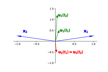
Figure 1: For time $t$ we denote $\mathbf{u}_{i}(t)=v_{i}(t)\mathbf{w}_{i}(t)$. Above we illustrate $\mathbf{u}_{1}(t),\mathbf{u}_{2}(t)$ for times $t_{1}<t_{2}$. As $t\to\infty$ we have $\left\|\mathbf{u}_{1}(t)\right\|\to\infty$ and $\mathbf{u}_{1}$ converges in direction to $(0,1)$. The vector $\mathbf{u}_{2}$ remains constant during the training. Hence $\frac{\mathbf{u}_{2}(t)}{\left\|{\boldsymbol{\theta}}(t)\right\|}\to{\mathbf{0}}$.

We note that the assumption on the initialization in the above theorem holds with constant probability for standard initialization schemes (e.g., Xavier initialization).

Remark 3.1 (Unbounded sub-optimality).

By choosing appropriate inputs $\mathbf{x}_{1},\mathbf{x}_{2}$ in the setting of Theorem 3.2, it is not hard to show that the sub-optimality of the KKT point w.r.t. the global optimum can be arbitrarily large. Namely, for every large $M>0$ we can choose a dataset where the angle between $\mathbf{x}_{1}$ and $\mathbf{x}_{2}$ is sufficiently close to $\pi$, such that $\frac{\|\tilde{{\boldsymbol{\theta}}}\|}{\|{\boldsymbol{\theta}}^{*}\|}\geq M$, where $\tilde{{\boldsymbol{\theta}}}$ is a KKT point to which gradient flow converges, and ${\boldsymbol{\theta}}^{*}$ is a global optimum of Problem 2. Indeed, as illustrated in Figure 1, if one neuron is active on both inputs and the other neuron is not active on any input, then the active neuron needs to be very large in order to achieve margin $1$, while if each neuron is active on a single input then we can achieve margin $1$ with much smaller parameters. We note that such unbounded sub-optimality can be obtained also in other negative results in this work (in Theorems 4.1, 4.3, 4.4 and 5.4).

Remark 3.2 (Robustness to small perturbations).

Theorem 3.2 holds even if we slightly perturb the inputs $\mathbf{x}_{1},\mathbf{x}_{2}$. Thus, it is not sensitive to small changes in the dataset. We note that such robustness to small perturbations can be shown also for the negative results in Theorems 4.1, 4.3, 5.1 and 5.4.

4 Depth-$2$ networks in ${\cal N}$

In this section we study depth-$2$ linear and ReLU networks in ${\cal N}$. We first show that already for linear networks in ${\cal N}_{\text{no-share}}$ (more specifically, for diagonal networks) gradient flow may not converge even to a local optimum.

Theorem 4.1.

Let $\Phi$ be a depth-$2$ linear or ReLU diagonal neural network parameterized by ${\boldsymbol{\theta}}=[\mathbf{w}_{1},\mathbf{w}_{2}]$. Consider minimizing either the exponential or the logistic loss using gradient flow. There exists a dataset $\{(\mathbf{x},y)\}\subseteq{\mathbb{R}}^{2}\times\{-1,1\}$ of size $1$ and an initialization ${\boldsymbol{\theta}}(0)$, such that gradient flow converges to zero loss, and converges in direction to a KKT point $\tilde{{\boldsymbol{\theta}}}$ of Problem 2 which is not a local optimum.

Proof idea (for the complete proof see Appendix C.4).

Let $\mathbf{x}=(1,2)^{\top}$ and $y=1$. Let ${\boldsymbol{\theta}}(0)$ such that $\mathbf{w}_{1}(0)=\mathbf{w}_{2}(0)=(1,0)^{\top}$. Recalling that the diagonal network computes the function $\mathbf{x}\mapsto(\mathbf{w}_{1}\circ\mathbf{w}_{2})^{\top}\mathbf{x}$ (where $\circ$ is the entry-wise product), we see that the second coordinate remains inactive during training. It is not hard to show that gradient flow converges in direction to the KKT point $\tilde{{\boldsymbol{\theta}}}$ with $\tilde{\mathbf{w}}_{1}=\tilde{\mathbf{w}}_{2}=(1,0)^{\top}$. However, it is not a local optimum, since for every small $\epsilon>0$ the parameters ${\boldsymbol{\theta}}^{\prime}=[\mathbf{w}^{\prime}_{1},\mathbf{w}^{\prime}_{2}]$ with $\mathbf{w}^{\prime}_{1}=\mathbf{w}^{\prime}_{2}=\left(\sqrt{1-\epsilon},\sqrt{\frac{\epsilon}{2}}\right)^{\top}$ satisfy the constraints of Problem 2, and we have $\|{\boldsymbol{\theta}}^{\prime}\|<\|\tilde{{\boldsymbol{\theta}}}\|$. ∎

By Theorem 3.2 fully-connected ReLU networks may not converge to a local optimum, and by Theorem 4.1 linear (and ReLU) networks with sparse weights may not converge to a local optimum. In the proofs of both of these negative results, gradient flow converges in direction to a KKT point such that one of the weights vectors of the hidden neurons is zero. However, in practice gradient descent often converges to a network that does not contain such disconnected neurons. Hence, a natural question is whether the negative results hold also in networks that do not contain neurons whose weights vector is zero. In the following theorem we show that in linear networks such an assumption allows us to obtain a positive result. Namely, in depth-$2$ linear networks in ${\cal N}_{\text{no-share}}$, if gradient flow converges in direction to a KKT point of Problem 2 that satisfies this condition, then it is guaranteed to be a global optimum. However, we also show that in ReLU networks assuming that all neurons have non-zero weights is not sufficient.

Theorem 4.2.

We have:

1. Let $\Phi$ be a depth-$2$ linear neural network in ${\cal N}_{\text{no-share}}$ parameterized by ${\boldsymbol{\theta}}$. Consider minimizing either the exponential or the logistic loss over a dataset $\{(\mathbf{x}_{i},y_{i})\}_{i=1}^{n}$ using gradient flow. Assume that there exists time $t_{0}$ such that ${\cal L}({\boldsymbol{\theta}}(t_{0}))<1$, and let $\tilde{{\boldsymbol{\theta}}}$ be the KKT point of Problem 2 such that ${\boldsymbol{\theta}}(t)$ converges to $\tilde{{\boldsymbol{\theta}}}$ in direction (such $\tilde{{\boldsymbol{\theta}}}$ exists by Theorem 2.1). Assume that in the network parameterized by $\tilde{{\boldsymbol{\theta}}}$ all hidden neurons have non-zero incoming weights vectors. Then, $\tilde{{\boldsymbol{\theta}}}$ is a global optimum of Problem 2.

2. Let $\Phi$ be a fully-connected depth-$2$ ReLU network with input dimension $2$ and $4$ hidden neurons parameterized by ${\boldsymbol{\theta}}$. Consider minimizing either the exponential or the logistic loss using gradient flow. There exists a dataset and an initialization ${\boldsymbol{\theta}}(0)$, such that gradient flow converges to zero loss, and converges in direction to a KKT point $\tilde{{\boldsymbol{\theta}}}$ of Problem 2, which is not a local optimum, and in the network parameterized by $\tilde{{\boldsymbol{\theta}}}$ all hidden neurons have non-zero incoming weights.

Proof idea (for the complete proof see Appendix C.5).

We give here the proof idea for part (1). Let $k$ be the width of the network. For every $j\in[k]$ we denote by $\mathbf{w}_{j}$ the incoming weights vector to the $j$-th hidden neuron, and by $v_{j}$ the outgoing weight. Let $\mathbf{u}_{j}=v_{j}\mathbf{w}_{j}$. We consider an optimization problem over the variables $\mathbf{u}_{1},\ldots,\mathbf{u}_{k}$ where the objective is to minimize $\sum_{j\in[k]}\left\|\mathbf{u}_{j}\right\|$ and the constrains correspond to the constraints of Problem 2. Let $\tilde{{\boldsymbol{\theta}}}=[\tilde{\mathbf{w}}_{1},\ldots,\tilde{\mathbf{w}}_{k},\tilde{\mathbf{v}}]$ be the KKT point of Problem 2 to which gradient flow converges in direction. For every $j\in[k]$ we denote $\tilde{\mathbf{u}}_{j}=\tilde{v}_{j}\tilde{\mathbf{w}}_{j}$. We show that $\tilde{\mathbf{u}}_{1},\ldots,\tilde{\mathbf{u}}_{k}$ satisfy the KKT conditions of the aforementioned problem. Since the objective there is convex and the constrains are affine, then it is a global optimum. Finally, we show that it implies global optimality of $\tilde{{\boldsymbol{\theta}}}$. ∎

Remark 4.1 (Implications on margin maximization in predictor space for diagonal linear networks).

Theorems 4.1 and 4.2 imply analogous results on diagonal linear networks also in predictor space. As we discussed in Section 2, Gunasekar et al. (2018b) showed that in depth-$2$ diagonal linear networks, minimizing $\left\|{\boldsymbol{\theta}}\right\|_{2}$ under the constraints in Problem 2 implies minimizing $\left\|\boldsymbol{\beta}\right\|_{1}$, where $\boldsymbol{\beta}$ is the corresponding linear predictor. Theorem 4.1 can be easily extended to predictor space, namely, gradient flow on depth-$2$ linear diagonal networks might converge to a KKT point $\tilde{{\boldsymbol{\theta}}}$ of Problem 2, such that the corresponding linear predictor $\tilde{\boldsymbol{\beta}}$ is not an optimum of the following problem:

$$\operatorname*{argmin}_{\boldsymbol{\beta}}\left\|\boldsymbol{\beta}\right\|_{1}\;\;\;\;\text{s.t. }\;\;\;\forall i\in[n]\;\;y_{i}\langle\boldsymbol{\beta},\mathbf{x}_{i}\rangle\geq 1~{}.$$ (3)

Moreover, by combining part (1) of Theorem 4.2 with the result from Gunasekar et al. (2018b), we deduce that if gradient flow on a depth-$2$ diagonal linear network converges in direction to a KKT point $\tilde{{\boldsymbol{\theta}}}$ of Problem 2 with non-zero weights vectors, then the corresponding linear predictor is a global optimum of Problem 3.

We argue that since in practice gradient descent often converges to networks without zero-weight neurons, then part (1) of Theorem 4.2 gives a useful positive result for depth-$2$ linear networks. However, by part (2) of Theorem 4.2, this assumption is not sufficient for obtaining a positive result in the case of ReLU networks. Hence, we now consider a stronger assumption, namely, that the KKT point $\tilde{{\boldsymbol{\theta}}}$ is such that for every $\mathbf{x}_{i}$ in the dataset the inputs to all hidden neurons in the computation $\Phi(\tilde{{\boldsymbol{\theta}}};\mathbf{x}_{i})$ are non-zero. In the following theorem we show that in depth-$2$ ReLU networks, if the KKT point satisfies this condition then it is guaranteed to be a local optimum of Problem 2. However, even under this condition it is not necessarily a global optimum. The proof is given in Appendix C.6 and uses ideas from the previous proofs, with some required modifications.

Theorem 4.3.

Let $\Phi$ be a depth-$2$ ReLU network in ${\cal N}_{\text{no-share}}$ parameterized by ${\boldsymbol{\theta}}$. Consider minimizing either the exponential or the logistic loss over a dataset $\{(\mathbf{x}_{i},y_{i})\}_{i=1}^{n}$ using gradient flow. Assume that there exists time $t_{0}$ such that ${\cal L}({\boldsymbol{\theta}}(t_{0}))<1$, and let $\tilde{{\boldsymbol{\theta}}}$ be the KKT point of Problem 2 such that ${\boldsymbol{\theta}}(t)$ converges to $\tilde{{\boldsymbol{\theta}}}$ in direction (such $\tilde{{\boldsymbol{\theta}}}$ exists by Theorem 2.1). Assume that for every $i\in[n]$ the inputs to all hidden neurons in the computation $\Phi(\tilde{{\boldsymbol{\theta}}};\mathbf{x}_{i})$ are non-zero. Then, $\tilde{{\boldsymbol{\theta}}}$ is a local optimum of Problem 2. However, it may not be a global optimum, even if the network $\Phi$ is fully connected.

Note that in all the above theorems we do not allow shared weights. We now consider the case of depth-$2$ linear or ReLU networks in ${\cal N}$, where the first layer is convolutional with disjoint patches (and hence has shared weights), and show that gradient flow does not always converge in direction to a local optimum, even when the inputs to all hidden neurons are non-zero (and hence there are no zero weights vectors).

Theorem 4.4.

Let $\Phi$ be a depth-$2$ linear or ReLU network in ${\cal N}$, parameterized by ${\boldsymbol{\theta}}=[\mathbf{w},\mathbf{v}]$ for $\mathbf{w},\mathbf{v}\in{\mathbb{R}}^{2}$, such that for $\mathbf{x}\in{\mathbb{R}}^{4}$ we have $\Phi({\boldsymbol{\theta}};\mathbf{x})=\sum_{j=1}^{2}v_{j}\sigma(\mathbf{w}^{\top}\mathbf{x}^{(j)})$ where $\mathbf{x}^{(1)}=(x_{1},x_{2})$ and $\mathbf{x}^{(2)}=(x_{3},x_{4})$. Thus, $\Phi$ is a convolutional network with two disjoint patches. Consider minimizing either the exponential or the logistic loss using gradient flow. Then, there exists a dataset $\{(\mathbf{x},y)\}$ of size $1$, and an initialization ${\boldsymbol{\theta}}(0)$, such that gradient flow converges to zero loss, and converges in direction to a KKT point $\tilde{{\boldsymbol{\theta}}}=[\tilde{\mathbf{w}},\tilde{\mathbf{v}}]$ of Problem 2 which is not a local optimum. Moreover, we have $\langle\tilde{\mathbf{w}},\mathbf{x}^{(j)}\rangle\neq 0$ for $j\in\{1,2\}$.

Proof idea (for the complete proof see Appendix C.7).

Let $\mathbf{x}=\left(4,\frac{1}{\sqrt{2}},-4,\frac{1}{\sqrt{2}}\right)^{\top}$ and $y=1$. Let ${\boldsymbol{\theta}}(0)$ such that $\mathbf{w}(0)=(0,1)^{\top}$ and $\mathbf{v}(0)=\left(\frac{1}{\sqrt{2}},\frac{1}{\sqrt{2}}\right)^{\top}$. Since $\mathbf{x}^{(1)}$ and $\mathbf{x}^{(2)}$ are symmetric w.r.t. $\mathbf{w}(0)$, and $\mathbf{v}(0)$ does not break this symmetry, then $\mathbf{w}$ keeps its direction throughout the training. Thus, we show that gradient flow converges in direction to a KKT point $\tilde{{\boldsymbol{\theta}}}$ where $\tilde{\mathbf{w}}=(0,1)^{\top}$ and $\tilde{\mathbf{v}}=\left(\frac{1}{\sqrt{2}},\frac{1}{\sqrt{2}}\right)^{\top}$. Then, we show that it is not a local optimum, since for every small $\epsilon>0$ the parameters ${\boldsymbol{\theta}}^{\prime}=[\mathbf{w}^{\prime},\mathbf{v}^{\prime}]$ with $\mathbf{w}^{\prime}=(\sqrt{\epsilon},1-\epsilon)^{\top}$ and $\mathbf{v}^{\prime}=\left(\frac{1}{\sqrt{2}}+\frac{\sqrt{\epsilon}}{2},\frac{1}{\sqrt{2}}-\frac{\sqrt{\epsilon}}{2}\right)^{\top}$ satisfy the constraints of Problem 2, and we have $\|{\boldsymbol{\theta}}^{\prime}\|<\|\tilde{{\boldsymbol{\theta}}}\|$. ∎

5 Deep networks in ${\cal N}$

In this section we study the more general case of depth-$m$ neural networks in ${\cal N}$, where $m\geq 2$. First, we show that for networks of depth at least $3$ in ${\cal N}_{\text{no-share}}$, gradient flow may not converge to a local optimum of Problem 2, for both linear and ReLU networks, and even where there are no zero weights vectors and the inputs to all hidden neurons are non-zero. More precisely, we prove this claim for diagonal networks.

Theorem 5.1.

Let $m\geq 3$. Let $\Phi$ be a depth-$m$ linear or ReLU diagonal neural network parameterized by ${\boldsymbol{\theta}}$. Consider minimizing either the exponential or the logistic loss using gradient flow. There exists a dataset $\{(\mathbf{x},y)\}\subseteq{\mathbb{R}}^{2}\times\{-1,1\}$ of size $1$ and an initialization ${\boldsymbol{\theta}}(0)$, such that gradient flow converges to zero loss, and converges in direction to a KKT point $\tilde{{\boldsymbol{\theta}}}$ of Problem 2 which is not a local optimum. Moreover, all inputs to neurons in the computation $\Phi(\tilde{{\boldsymbol{\theta}}};\mathbf{x})$ are non-zero.

Proof idea (for the complete proof see Appendix C.8).

Let $\mathbf{x}=(1,1)^{\top}$ and $y=1$. Consider the initialization ${\boldsymbol{\theta}}(0)$ where $\mathbf{w}_{j}(0)=(1,1)^{\top}$ for every $j\in[m]$. We show that gradient flow converges in direction to a KKT point $\tilde{{\boldsymbol{\theta}}}=[\tilde{\mathbf{w}}_{1},\ldots,\tilde{\mathbf{w}}_{m}]$ such that $\tilde{\mathbf{w}}_{j}=\left(2^{-1/m},2^{-1/m}\right)^{\top}$ for all $j\in[m]$. Then, we consider the parameters ${\boldsymbol{\theta}}^{\prime}=[\mathbf{w}^{\prime}_{1},\ldots,\mathbf{w}^{\prime}_{m}]$ such that for every $j\in[m]$ we have $\mathbf{w}^{\prime}_{j}=\left(\left(\frac{1+\epsilon}{2}\right)^{1/m},\left(\frac{1-\epsilon}{2}\right)^{1/m}\right)^{\top}$, and show that if $\epsilon>0$ is sufficiently small, then ${\boldsymbol{\theta}}^{\prime}$ satisfies the constraints in Problem 2 and we have $\|{\boldsymbol{\theta}}^{\prime}\|<\|\tilde{{\boldsymbol{\theta}}}\|$. ∎

Note that in the case of linear networks, the above result is in contrast to networks with sparse weights of depth $2$ that converge to a global optimum by Theorem 4.2, and to fully-connected networks of any depth that converge to a global optimum by Theorem 3.1. In the case of ReLU networks, the above result is in contrast to the case of depth-$2$ networks studied in Theorem 4.3, where it is guaranteed to converge to a local optimum.

In light of our negative results, we now consider a weaker notion of margin maximization, namely, maximizing the margin for each layer separately. Let $\Phi$ be a neural network of depth $m$ in ${\cal N}$, parameterized by ${\boldsymbol{\theta}}=[\mathbf{u}^{(l)}]_{l=1}^{m}$. The maximum margin problem for a layer $l_{0}\in[m]$ w.r.t. ${\boldsymbol{\theta}}_{0}=[\mathbf{u}^{(l)}_{0}]_{l=1}^{m}$ is the following:

$$\min_{\mathbf{u}^{(l_{0})}}\frac{1}{2}\left\|\mathbf{u}^{(l_{0})}\right\|^{2}\;\;\;\;\text{s.t. }\;\;\;\forall i\in[n]\;\;y_{i}\Phi({\boldsymbol{\theta}}^{\prime};\mathbf{x}_{i})\geq 1~{},$$ (4)

where ${\boldsymbol{\theta}}^{\prime}=[\mathbf{u}^{(1)}_{0},\ldots,\mathbf{u}^{(l_{0}-1)}_{0},\mathbf{u}^{(l_{0})},\mathbf{u}^{(l_{0}+1)}_{0},\ldots,\mathbf{u}^{(m)}_{0}]$. We show a positive result for linear networks:

Theorem 5.2.

Let $m\geq 2$. Let $\Phi$ be any depth-$m$ linear neural network in ${\cal N}$, parameterized by ${\boldsymbol{\theta}}=[\mathbf{u}^{(l)}]_{l=1}^{m}$. Consider minimizing either the exponential or the logistic loss over a dataset $\{(\mathbf{x}_{i},y_{i})\}_{i=1}^{n}$ using gradient flow. Assume that there exists time $t_{0}$ such that ${\cal L}({\boldsymbol{\theta}}(t_{0}))<1$. Then, gradient flow converges in direction to a KKT point $\tilde{{\boldsymbol{\theta}}}=[\tilde{\mathbf{u}}^{(l)}]_{l=1}^{m}$ of Problem 2, such that for every layer $l\in[m]$ the parameters vector $\tilde{\mathbf{u}}^{(l)}$ is a global optimum of Problem 4 w.r.t. $\tilde{{\boldsymbol{\theta}}}$.

The theorem follows by noticing that if $\Phi$ is a linear network, then the constraints in Problem 4 are affine, and its KKT conditions are implied by the KKT conditions of Problem 2. See Appendix C.9 for the formal proof. Note that by Theorems 4.1, 4.4 and 5.1, linear networks in ${\cal N}$ might converge in direction to a KKT point $\tilde{{\boldsymbol{\theta}}}$, which is not a local optimum of Problem 2. However, Theorem 5.2 implies that each layer in $\tilde{{\boldsymbol{\theta}}}$ is a global optimum of Problem 4. Hence, any improvement to $\tilde{{\boldsymbol{\theta}}}$ requires changing at least two layers simultaneously.

While in linear networks gradient flow maximize the margin for each layer separately, in the following theorem (which we prove in Appendix C.10) we show that this claim does not hold for ReLU networks: Already for fully-connected networks of depth-$2$ gradient flow may not converge in direction to a local optimum of Problem 4.

Theorem 5.3.

Let $\Phi$ be a fully-connected depth-$2$ ReLU network with input dimension $2$ and $4$ hidden neurons parameterized by ${\boldsymbol{\theta}}$. Consider minimizing either the exponential or the logistic loss using gradient flow. There exists a dataset and an initialization ${\boldsymbol{\theta}}(0)$ such that gradient flow converges to zero loss, and converges in direction to a KKT point $\tilde{{\boldsymbol{\theta}}}$ of Problem 2, such that the weights of the first layer are not a local optimum of Problem 4 w.r.t. $\tilde{{\boldsymbol{\theta}}}$.

Finally, we show that in ReLU networks in ${\cal N}$ of any depth, if the KKT point to which gradient flow converges in direction is such that the inputs to hidden neurons are non-zero, then it must be a local optimum of Problem 4 (but not necessarily a global optimum). The proof follows the ideas from the proof of Theorem 5.2, with some required modifications, and is given in Appendix C.11.

Theorem 5.4.

Let $m\geq 2$. Let $\Phi$ be any depth-$m$ ReLU network in ${\cal N}$ parameterized by ${\boldsymbol{\theta}}=[\mathbf{u}^{(l)}]_{l=1}^{m}$. Consider minimizing either the exponential or the logistic loss over a dataset $\{(\mathbf{x}_{i},y_{i})\}_{i=1}^{n}$ using gradient flow, and assume that there exists time $t_{0}$ such that ${\cal L}({\boldsymbol{\theta}}(t_{0}))<1$. Let $\tilde{{\boldsymbol{\theta}}}=[\tilde{\mathbf{u}}^{(l)}]_{l=1}^{m}$ be the KKT point of Problem 2 such that ${\boldsymbol{\theta}}(t)$ converges to $\tilde{{\boldsymbol{\theta}}}$ in direction (such $\tilde{{\boldsymbol{\theta}}}$ exists by Theorem 2.1). Let $l\in[m]$ and assume that for every $i\in[n]$ the inputs to all neurons in layers $\geq l$ in the computation $\Phi(\tilde{{\boldsymbol{\theta}}};\mathbf{x}_{i})$ are non-zero. Then, the parameters vector $\tilde{\mathbf{u}}^{(l)}$ is a local optimum of Problem 4 w.r.t. $\tilde{{\boldsymbol{\theta}}}$. However, it may not be a global optimum.

Acknowledgements

This research is supported in part by European Research Council (ERC) grant 754705.

Appendix A Additional related work

Soudry et al. [2018] showed that gradient descent on linearly-separable binary classification problems with exponentially-tailed losses (e.g., the exponential loss and the logistic loss), converges to the maximum $\ell_{2}$-margin direction. This analysis was extended to other loss functions, tighter convergence rates, non-separable data, and variants of gradient-based optimization algorithms [Nacson et al., 2019, Ji and Telgarsky, 2018b, Ji et al., 2020, Gunasekar et al., 2018a, Shamir, 2020, Ji and Telgarsky, 2021].

As detailed in Section 2, Lyu and Li [2019] and Ji and Telgarsky [2020] showed that gradient flow on homogeneous neural networks with exponential-type losses converge in direction to a KKT point of the maximum-margin problem in parameter space. The implications of margin maximization in parameter space on the implicit bias in predictor space for linear neural networks were studied in Gunasekar et al. [2018b] (as detailed in Section 2) and also in Jagadeesan et al. [2021], Ergen and Pilanci [2021a, b]. Moreover, several recent works considered implications of convergence to a KKT point of the maximum-margin problem, without assuming that the KKT point is optimal: Safran et al. [2022] proved a generalization bound in univariate depth-$2$ ReLU networks, Vardi et al. [2022] proved bias towards non-robust solutions in depth-$2$ ReLU networks, and Haim et al. [2022] showed that training data can be reconstructed from trained networks. Margin maximization in predictor space for fully-connected linear networks was shown by Ji and Telgarsky [2020] (as detailed in Section 2), and similar results under stronger assumptions were previously established in Gunasekar et al. [2018b] and in Ji and Telgarsky [2018a]. The implicit bias in predictor space of diagonal and convolutional linear networks was studied in Gunasekar et al. [2018b], Moroshko et al. [2020], Yun et al. [2020]. Chizat and Bach [2020] studied the dynamics of gradient flow on infinite-width homogeneous two-layer networks with exponentially-tailed losses, and showed bias towards margin maximization w.r.t. a certain function norm known as the variation norm. Sarussi et al. [2021] studied gradient flow on two-layer leaky-ReLU networks, where the training data is linearly separable, and showed convergence to a linear classifier based on a certain assumption called Neural Agreement Regime (NAR). Phuong and Lampert [2020] studied the implicit bias in depth-$2$ ReLU networks trained on orthogonally-separable data.

Lyu et al. [2021] studied the implicit bias in two-layer leaky-ReLU networks trained on linearly separable and symmetric data, and showed that gradient flow converges to a linear classifier which maximizes the $\ell_{2}$ margin. They also gave constructions where a KKT point is not a global max-margin solution. We note that their constructions do not imply any of our results. In particular, for the ReLU activation they showed a construction where there exists a KKT point which is not a global optimum of the max-margin problem, however this KKT point is not reachable with gradient flow. Thus, there does not exist an initialization such that gradient flow actually converges to this point. In our construction (Theorem 3.2) gradient flow converges to a suboptimal KKT point with constant probability over the initialization. Moreover, even their construction for the leaky-ReLU activation (which is their main focus) considers only global suboptimality, while we show local suboptimality for the ReLU activation.

Finally, the implicit bias of neural networks in regression tasks w.r.t. the square loss was also extensively studied in recent years (e.g., Gunasekar et al. [2018c], Razin and Cohen [2020], Arora et al. [2019], Belabbas [2020], Eftekhari and Zygalakis [2020], Li et al. [2018], Ma et al. [2018], Woodworth et al. [2020], Gidel et al. [2019], Li et al. [2020], Yun et al. [2020], Vardi and Shamir [2021], Azulay et al. [2021], Timor et al. [2022]). This setting, however, is less relevant to our work.

For a broader discussion on the implicit bias in neural networks, in both classification and regression tasks, see a survey in Vardi [2022].

Appendix B Preliminaries on the KKT conditions

Below we review the definition of the KKT condition for non-smooth optimization problems (cf. Lyu and Li [2019], Dutta et al. [2013]).

Let $f:{\mathbb{R}}^{d}\to{\mathbb{R}}$ be a locally Lipschitz function. The Clarke subdifferential [Clarke et al., 2008] at $\mathbf{x}\in{\mathbb{R}}^{d}$ is the convex set

$$\partial^{\circ}f(\mathbf{x}):=\text{conv}\left\{\lim_{i\to\infty}\nabla f(\mathbf{x}_{i})\;\middle|\;\lim_{i\to\infty}\mathbf{x}_{i}=\mathbf{x},\;f\text{ is differentiable at }\mathbf{x}_{i}\right\}~{}.$$

If $f$ is continuously differentiable at $\mathbf{x}$ then $\partial^{\circ}f(\mathbf{x})=\{\nabla f(\mathbf{x})\}$.

Consider the following optimization problem

$$\min f(\mathbf{x})\;\;\;\;\text{s.t. }\;\;\;\forall n\in[N]\;\;g_{n}(\mathbf{x})\leq 0~{},$$ (5)

where $f,g_{1},\ldots,g_{n}:{\mathbb{R}}^{d}\to{\mathbb{R}}$ are locally Lipschitz functions. We say that $\mathbf{x}\in{\mathbb{R}}^{d}$ is a feasible point of Problem 5 if $\mathbf{x}$ satisfies $g_{n}(\mathbf{x})\leq 0$ for all $n\in[N]$. We say that a feasible point $\mathbf{x}$ is a KKT point if there exists $\lambda_{1},\ldots,\lambda_{N}\geq 0$ such that

1. ${\mathbf{0}}\in\partial^{\circ}f(\mathbf{x})+\sum_{n\in[N]}\lambda_{n}\partial^{\circ}g_{n}(\mathbf{x})$;

2. For all $n\in[N]$ we have $\lambda_{n}g_{n}(\mathbf{x})=0$.

Appendix C Proofs

C.1 Auxiliary lemmas

Throughout our proofs we use the following two lemmas from Du et al. [2018]:

Lemma C.1 (Du et al. [2018]).

Let $m\geq 2$, and let $\Phi$ be a depth-$m$ fully-connected linear or ReLU network parameterized by ${\boldsymbol{\theta}}=[W_{1},\ldots,W_{m}]$. Suppose that for every $j\in[m]$ we have $W_{j}\in{\mathbb{R}}^{d_{j}\times d_{j-1}}$. Consider minimizing any differentiable loss function (e.g., the exponential or the logistic loss) over a dataset using gradient flow. Then, for every $j\in[m-1]$ at all time $t$ we have

$$\frac{d}{dt}\left(\left\|W_{j}\right\|_{F}^{2}-\left\|W_{j+1}\right\|_{F}^{2}\right)=0~{}.$$

Moreover, for every $j\in[m-1]$ and $i\in[d_{j}]$ we have

$$\frac{d}{dt}\left(\left\|W_{j}[i,:]\right\|^{2}-\left\|W_{j+1}[:,i]\right\|^{2}\right)=0~{},$$

where $W_{j}[i,:]$ is the vector of incoming weights to the $i$-th neuron in the $j$-th hidden layer (i.e., the $i$-th row of $W_{j}$), and $W_{j+1}[:,i]$ is the vector of outgoing weights from this neuron (i.e., the $i$-th column of $W_{j+1}$).

Lemma C.2 (Du et al. [2018]).

Let $m\geq 2$, and let $\Phi$ be a depth-$m$ linear or ReLU network in ${\cal N}$, parameterized by ${\boldsymbol{\theta}}=[\mathbf{u}^{(1)},\ldots,\mathbf{u}^{(m)}]$. Consider minimizing any differentiable loss function (e.g., the exponential or the logistic loss) over a dataset using gradient flow. Then, for every $j\in[m-1]$ at all time $t$ we have

$$\frac{d}{dt}\left(\left\|\mathbf{u}^{(j)}\right\|^{2}-\left\|\mathbf{u}^{(j+1)}\right\|^{2}\right)=0~{}.$$

Note that Lemma C.2 considers a larger family of neural networks since it allows sparse and shared weights, but Lemma C.1 gives a stronger guarantee, since it implies balancedness between the incoming and outgoing weights of each hidden neuron separately. In our proofs we will also need to use a balancedness property for each hidden neuron separately in depth-$2$ networks with sparse weights. Since this property is not implied by the above lemmas from Du et al. [2018], we now prove it.

Before stating the lemma, let us introduce some required notations. Let $\Phi$ be a depth-$2$ network in ${\cal N}_{\text{no-share}}$. We can always assume w.l.o.g. that the second layer is fully connected, namely, all hidden neurons are connected to the output neuron. Indeed, otherwise we can ignore the neurons that are not connected to the output neuron. For the network $\Phi$ we use the parameterization ${\boldsymbol{\theta}}=[\mathbf{w}_{1},\ldots,\mathbf{w}_{k},\mathbf{v}]$, where $k$ is the number of hidden neurons. For every $j\in[k]$ the vector $\mathbf{w}_{j}\in{\mathbb{R}}^{p_{j}}$ is the weights vector of the $j$-th hidden neuron, and we have $1\leq p_{j}\leq d$ where $d$ is the input dimention. For an input $\mathbf{x}\in{\mathbb{R}}^{d}$ we denote by $\mathbf{x}^{j}\in{\mathbb{R}}^{p_{j}}$ a sub-vector of $\mathbf{x}$, such that $\mathbf{x}^{j}$ includes the coordinates of $\mathbf{x}$ that are connected to the $j$-th hidden neuron. Thus, given $\mathbf{x}$, the input to the $j$-th hidden neuron is $\langle\mathbf{w}_{j},\mathbf{x}^{j}\rangle$. The vector $\mathbf{v}\in{\mathbb{R}}^{k}$ is the weights vector of the second layer. Overall, we have $\Phi({\boldsymbol{\theta}};\mathbf{x})=\sum_{j\in[k]}v_{j}\sigma(\mathbf{w}_{j}^{\top}\mathbf{x}^{j})$.

Lemma C.3.

Let $\Phi$ be a depth-$2$ linear or ReLU network in ${\cal N}_{\text{no-share}}$, parameterized by ${\boldsymbol{\theta}}=[\mathbf{w}_{1},\ldots,\mathbf{w}_{k},\mathbf{v}]$. Consider minimizing any differentiable loss function (e.g., the exponential or the logistic loss) over a dataset using gradient flow. Then, for every $j\in[k]$ at all time $t$ we have

$$\frac{d}{dt}\left(\left\|\mathbf{w}_{j}\right\|^{2}-v_{j}^{2}\right)=0~{}.$$

Proof.

We have

$${\cal L}({\boldsymbol{\theta}})=\sum_{i\in[n]}\ell\left(y_{i}\Phi({\boldsymbol{\theta}};\mathbf{x}_{i})\right)=\sum_{i\in[n]}\ell\left(y_{i}\sum_{l\in[k]}v_{l}\sigma(\mathbf{w}_{l}^{\top}\mathbf{x}_{i}^{j})\right)~{}.$$

Hence

$$\frac{d}{dt}\left(\left\|\mathbf{w}_{j}\right\|^{2}\right) =2\langle\mathbf{w}_{j},\frac{d\mathbf{w}_{j}}{dt}\rangle=-2\langle\mathbf{w}_{j},\nabla_{\mathbf{w}_{j}}{\cal L}({\boldsymbol{\theta}})\rangle$$

$$=-2\sum_{i\in[n]}\ell^{\prime}\left(y_{i}\sum_{l\in[k]}v_{l}\sigma(\mathbf{w}_{l}^{\top}\mathbf{x}_{i}^{l})\right)\cdot y_{i}v_{j}\sigma^{\prime}(\mathbf{w}_{j}^{\top}\mathbf{x}_{i}^{j})\mathbf{w}_{j}^{\top}\mathbf{x}_{i}^{j}$$

$$=-2\sum_{i\in[n]}\ell^{\prime}\left(y_{i}\sum_{l\in[k]}v_{l}\sigma(\mathbf{w}_{l}^{\top}\mathbf{x}_{i}^{l})\right)\cdot y_{i}v_{j}\sigma(\mathbf{w}_{j}^{\top}\mathbf{x}_{i}^{j})~{}.$$

Moreover,

$$\frac{d}{dt}\left(v_{j}^{2}\right) =2v_{j}\frac{dv_{j}}{dt}=-2v_{j}\nabla_{v_{j}}{\cal L}({\boldsymbol{\theta}})$$

$$=-2v_{j}\sum_{i\in[n]}\ell^{\prime}\left(y_{i}\sum_{l\in[k]}v_{l}\sigma(\mathbf{w}_{l}^{\top}\mathbf{x}_{i}^{l})\right)\cdot y_{i}\sigma(\mathbf{w}_{j}^{\top}\mathbf{x}_{i}^{j})~{}.$$

Hence the lemma follows. ∎

Using the above lemma, we show the following:

Lemma C.4.

Let $\Phi$ be a depth-$2$ linear or ReLU network in ${\cal N}_{\text{no-share}}$, parameterized by ${\boldsymbol{\theta}}=[\mathbf{w}_{1},\ldots,\mathbf{w}_{k},\mathbf{v}]$. Consider minimizing any differentiable loss function (e.g., the exponential or the logistic loss) over a dataset using gradient flow starting from ${\boldsymbol{\theta}}(0)$. Assume that $\lim_{t\to\infty}\left\|{\boldsymbol{\theta}}(t)\right\|=\infty$ and that ${\boldsymbol{\theta}}(t)$ converges in direction to $\tilde{{\boldsymbol{\theta}}}=[\tilde{\mathbf{w}}_{1},\ldots,\tilde{\mathbf{w}}_{k},\tilde{\mathbf{v}}]$, i.e., $\tilde{{\boldsymbol{\theta}}}=\|\tilde{{\boldsymbol{\theta}}}\|\cdot\lim_{t\to\infty}\frac{{\boldsymbol{\theta}}(t)}{\left\|{\boldsymbol{\theta}}(t)\right\|}$. Then, for every $l\in[k]$ we have $\left\|\tilde{\mathbf{w}}_{l}\right\|=|\tilde{v}_{l}|$.

Proof.

For every $l\in[k]$, let $\Delta_{l}=\left\|\mathbf{w}_{l}(0)\right\|^{2}-v_{l}(0)^{2}$. By Lemma C.3, we have for every $l\in[k]$ and $t\geq 0$ that $\left\|\mathbf{w}_{l}(t)\right\|^{2}-v_{l}(t)^{2}=\Delta_{l}$, namely, the differences between the square norms of the incoming and outgoing weights of each hidden neuron remain constant during the training. Hence, we have

$$|\tilde{v}_{l}|=\|\tilde{{\boldsymbol{\theta}}}\|\cdot\lim_{t\to\infty}\frac{|v_{l}(t)|}{\left\|{\boldsymbol{\theta}}(t)\right\|}=\|\tilde{{\boldsymbol{\theta}}}\|\cdot\lim_{t\to\infty}\frac{\sqrt{\left\|\mathbf{w}_{l}(t)\right\|^{2}-\Delta_{l}}}{\left\|{\boldsymbol{\theta}}(t)\right\|}~{}.$$

Thus, if $\lim_{t\to\infty}\left\|\mathbf{w}_{l}(t)\right\|=\infty$, then we have $|\tilde{v}_{l}|=\|\tilde{{\boldsymbol{\theta}}}\|\cdot\lim_{t\to\infty}\frac{\left\|\mathbf{w}_{l}(t)\right\|}{\left\|{\boldsymbol{\theta}}(t)\right\|}=\left\|\tilde{\mathbf{w}}_{l}\right\|$.

Assume now that $\left\|\mathbf{w}_{l}(t)\right\|\not\to\infty$. By the definition of $\tilde{{\boldsymbol{\theta}}}$ we have $\left\|\tilde{\mathbf{w}}_{l}\right\|=\|\tilde{{\boldsymbol{\theta}}}\|\cdot\lim_{t\to\infty}\frac{\left\|\mathbf{w}_{l}(t)\right\|}{\left\|{\boldsymbol{\theta}}(t)\right\|}$. Since $\lim_{t\to\infty}\frac{\left\|\mathbf{w}_{l}(t)\right\|}{\left\|{\boldsymbol{\theta}}(t)\right\|}$ exists and $\lim_{t\to\infty}\left\|{\boldsymbol{\theta}}(t)\right\|=\infty$, then we have $\lim_{t\to\infty}\frac{\left\|\mathbf{w}_{l}(t)\right\|}{\left\|{\boldsymbol{\theta}}(t)\right\|}=0$. Hence, $\lim_{t\to\infty}\frac{|v_{l}(t)|}{\left\|{\boldsymbol{\theta}}(t)\right\|}=\lim_{t\to\infty}\frac{\sqrt{\left\|\mathbf{w}_{l}(t)\right\|^{2}-\Delta_{l}}}{\left\|{\boldsymbol{\theta}}(t)\right\|}=0$. Therefore $\left\|\tilde{\mathbf{w}}_{l}\right\|=\tilde{v}_{l}=0$. ∎

C.2 Proof of Theorem 3.1

Suppose that the network $\Phi$ is parameterized by ${\boldsymbol{\theta}}=[W^{(1)},\ldots,W^{(m)}]$. By Theorem 2.1, gradient flow converges in direction to a KKT point $\tilde{{\boldsymbol{\theta}}}=[\tilde{W}^{(1)},\ldots,\tilde{W}^{(m)}]$ of Problem 2. For every $l\in[m]$ let $\Delta_{l}=\left\|W^{(l)}(0)\right\|_{F}^{2}-\left\|W^{(1)}(0)\right\|_{F}^{2}$. By Lemma C.1, we have for every $l\in[m]$ and $t\geq 0$ that

$$\left\|W^{(l)}(t)\right\|_{F}^{2}-\left\|W^{(1)}(t)\right\|_{F}^{2} =\sum_{j=1}^{l-1}\left\|W^{(j+1)}(t)\right\|_{F}^{2}-\left\|W^{(j)}(t)\right\|_{F}^{2}=\sum_{j=1}^{l-1}\left\|W^{(j+1)}(0)\right\|_{F}^{2}-\left\|W^{(j)}(0)\right\|_{F}^{2}$$

$$=\left\|W^{(l)}(0)\right\|_{F}^{2}-\left\|W^{(1)}(0)\right\|_{F}^{2}=\Delta_{l}~{}.$$

Hence, we have

$$\left\|\tilde{W}^{(l)}\right\|_{F}=\|\tilde{{\boldsymbol{\theta}}}\|\cdot\lim_{t\to\infty}\frac{\left\|W^{(l)}(t)\right\|_{F}}{\left\|{\boldsymbol{\theta}}(t)\right\|}=\|\tilde{{\boldsymbol{\theta}}}\|\cdot\lim_{t\to\infty}\frac{\sqrt{\left\|W^{(1)}(t)\right\|_{F}^{2}+\Delta_{l}}}{\left\|{\boldsymbol{\theta}}(t)\right\|}~{}.$$

Since by Theorem 2.1 we have $\lim_{t\to\infty}\left\|{\boldsymbol{\theta}}(t)\right\|=\infty$, then $\lim_{t\to\infty}\left\|W^{(1)}(t)\right\|_{F}=\infty$, and we have

$$\left\|\tilde{W}^{(l)}\right\|_{F}=\|\tilde{{\boldsymbol{\theta}}}\|\cdot\lim_{t\to\infty}\frac{\left\|W^{(1)}(t)\right\|_{F}}{\left\|{\boldsymbol{\theta}}(t)\right\|}=\left\|\tilde{W}^{(1)}\right\|_{F}:=C~{}.$$

By Ji and Telgarsky [2020] (Proposition 4.4), when gradient flow on a fully-connected linear network w.r.t. the exponential loss or the logistic loss converges to zero loss, then we have the following. There are unit vectors $\mathbf{v}_{0},\ldots,\mathbf{v}_{m}$ such that

$$\lim_{t\to\infty}\frac{W^{(l)}(t)}{\left\|W^{(l)}(t)\right\|_{F}}=\mathbf{v}_{l}\mathbf{v}_{l-1}^{\top}$$

for every $l\in[m]$. Moreover, we have $\mathbf{v}_{m}=1$, and $\mathbf{v}_{0}=\mathbf{u}$ where

$$\mathbf{u}:=\operatorname*{argmax}_{\left\|\mathbf{u}\right\|=1}\min_{i\in[n]}y_{i}\mathbf{u}^{\top}\mathbf{x}_{i}$$

is the unique linear max margin predictor.

Note that we have

$$\frac{\tilde{W}^{(l)}}{C}=\frac{\tilde{W}^{(l)}}{\left\|\tilde{W}^{(l)}\right\|_{F}}=\frac{\|\tilde{{\boldsymbol{\theta}}}\|\cdot\lim_{t\to\infty}\frac{W^{(l)}(t)}{\left\|{\boldsymbol{\theta}}(t)\right\|}}{\|\tilde{{\boldsymbol{\theta}}}\|\cdot\lim_{t\to\infty}\frac{\left\|W^{(l)}(t)\right\|_{F}}{\left\|{\boldsymbol{\theta}}(t)\right\|}}=\lim_{t\to\infty}\frac{W^{(l)}(t)}{\left\|W^{(l)}(t)\right\|_{F}}=\mathbf{v}_{l}\mathbf{v}_{l-1}^{\top}~{}.$$

Thus, $\tilde{W}^{(l)}=C\mathbf{v}_{l}\mathbf{v}_{l-1}^{\top}$ for every $l\in[m]$.

Let $\tilde{\mathbf{u}}=\tilde{W}^{(m)}\cdot\ldots\cdot\tilde{W}^{(1)}=C^{m}\mathbf{u}$. Since $\tilde{{\boldsymbol{\theta}}}$ is a KKT point of Problem 2, we have for every $l\in[m]$

$$\tilde{W}^{(l)}=\sum_{i\in[n]}\lambda_{i}y_{i}\frac{\partial\Phi(\tilde{{\boldsymbol{\theta}}};\mathbf{x}_{i})}{\partial W^{(l)}}~{},$$

where $\lambda_{i}\geq 0$ for every $i$, and $\lambda_{i}=0$ if $y_{i}\Phi(\tilde{{\boldsymbol{\theta}}};\mathbf{x}_{i})\neq 1$. Since $\tilde{W}^{(l)}$ are non-zero then there is $i\in[n]$ such that $1=y_{i}\Phi(\tilde{{\boldsymbol{\theta}}};\mathbf{x}_{i})=y_{i}\tilde{\mathbf{u}}^{\top}\mathbf{x}_{i}=y_{i}C^{m}\mathbf{u}^{\top}\mathbf{x}_{i}$. Likewise, since $\tilde{{\boldsymbol{\theta}}}$ satisfies the constraints of Problem 2, then for every $i\in[n]$ we have $1\leq y_{i}\Phi(\tilde{{\boldsymbol{\theta}}};\mathbf{x}_{i})=y_{i}C^{m}\mathbf{u}^{\top}\mathbf{x}_{i}$. Since, $\mathbf{u}$ is a unit vector that maximized the margin, then we have

$$\left\|\tilde{\mathbf{u}}\right\|=C^{m}=\min\left\|\mathbf{u}^{\prime}\right\|\text{ s.t. }y_{i}\mathbf{u}^{\prime\top}\mathbf{x}_{i}\geq 1\text{ for all }i\in[n]~{}.$$ (6)

Assume toward contradiction that there is ${\boldsymbol{\theta}}^{\prime}$ with $\|{\boldsymbol{\theta}}^{\prime}\|<\|\tilde{{\boldsymbol{\theta}}}\|$ that satisfies the constraints in Problem 2. Let $\mathbf{u}^{\prime}=W^{\prime(m)}\cdot\ldots\cdot W^{\prime(1)}$. By Eq. 6 we have $\|\mathbf{u}^{\prime}\|\geq\|\tilde{\mathbf{u}}\|=C^{m}$. Moreover, we have $\left\|\mathbf{u}^{\prime}\right\|=\left\|W^{\prime(m)}\cdot\ldots\cdot W^{\prime(1)}\right\|\leq\prod_{l\in[m]}\left\|W^{\prime(l)}\right\|_{F}$ due to the submultiplicativity of the Frobenius norm. Hence $\prod_{l\in[m]}\left\|W^{\prime(l)}\right\|_{F}\geq C^{m}$. The following lemma implies that

$$\left\|{\boldsymbol{\theta}}^{\prime}\right\|^{2}=\sum_{l\in[m]}\left\|W^{\prime(l)}\right\|_{F}^{2}\geq m\cdot C^{2}=\sum_{l\in[m]}\left\|\tilde{W}^{(l)}\right\|_{F}^{2}=\left\|\tilde{{\boldsymbol{\theta}}}\right\|^{2}$$

in contradiction to our assumption, and thus completes the proof.

Lemma C.5.

Let $a_{1},\ldots,a_{m}$ be real numbers such that $\prod_{j\in[m]}a_{j}\geq C^{m}$ for some $C\geq 0$. Then $\sum_{j\in[m]}a_{j}^{2}\geq m\cdot C^{2}$.

Proof.

It suffices to prove the claim for the case where $\prod_{j\in[m]}a_{j}=C^{m}$. Indeed, if $\prod_{j\in[m]}a_{j}>C^{m}$ then we can replace some $a_{j}$ with an appropriate $a^{\prime}_{j}$ such that $|a^{\prime}_{j}|<|a_{j}|$ and we only decrease $\sum_{j\in[m]}a_{j}^{2}$. Consider the following problem

$$\min\frac{1}{2}\sum_{j\in[m]}a_{j}^{2}\;\;\;\;\text{s.t. }\;\;\;\prod_{j\in[m]}a_{j}=C^{m}~{}.$$

Using the Lagrange multipliers we obtain that there is some $\lambda\in{\mathbb{R}}$ such that for every $l\in[m]$ we have $a_{l}=\lambda\cdot\prod_{j\neq l}a_{j}$. Thus, $a_{l}^{2}=\lambda\cdot\prod_{j\in[m]}a_{j}$. It implies that $a_{1}^{2}=\ldots=a_{m}^{2}$. Since $\prod_{j\in[m]}a_{j}=C^{m}$ then $|a_{j}|=C$ for every $j\in[m]$. Hence, $\sum_{j\in[m]}a_{j}^{2}=mC^{2}$. ∎

C.3 Proof of Theorem 3.2

Consider an initialization ${\boldsymbol{\theta}}(0)$ is such that $\mathbf{w}_{1}(0)$ satisfies $\langle\mathbf{w}_{1}(0),\mathbf{x}_{1}\rangle>0$ and $\langle\mathbf{w}_{1}(0),\mathbf{x}_{2}\rangle>0$, and $\mathbf{w}_{2}(0)$ satisfies $\langle\mathbf{w}_{2}(0),\mathbf{x}_{1}\rangle<0$ and $\langle\mathbf{w}_{2}(0),\mathbf{x}_{2}\rangle<0$. Moreover, assume that $v_{1}(0)>0$.

Note that for every ${\boldsymbol{\theta}}$ such that $\langle\mathbf{w}_{2},\mathbf{x}_{1}\rangle<0$ and $\langle\mathbf{w}_{2},\mathbf{x}_{2}\rangle<0$ we have

$$\nabla_{\mathbf{w}_{2}}{\cal L}({\boldsymbol{\theta}}) =\sum_{i=1}^{2}\ell^{\prime}(y_{i}\Phi({\boldsymbol{\theta}};\mathbf{x}_{i}))\cdot y_{i}\nabla_{\mathbf{w}_{2}}\Phi({\boldsymbol{\theta}};\mathbf{x}_{i})=\sum_{i=1}^{2}\ell^{\prime}(y_{i}\Phi({\boldsymbol{\theta}};\mathbf{x}_{i}))\cdot y_{i}\nabla_{\mathbf{w}_{2}}\left[v_{1}\sigma(\mathbf{w}_{1}^{\top}\mathbf{x}_{i})+v_{2}\sigma(\mathbf{w}_{2}^{\top}\mathbf{x}_{i})\right]$$

$$=\sum_{i=1}^{2}\ell^{\prime}(y_{i}\Phi({\boldsymbol{\theta}};\mathbf{x}_{i}))\cdot y_{i}v_{2}\sigma^{\prime}(\mathbf{w}_{2}^{\top}\mathbf{x}_{i})\mathbf{x}_{i}={\mathbf{0}}~{}.$$

and

$$\nabla_{v_{2}}{\cal L}({\boldsymbol{\theta}}) =\sum_{i=1}^{2}\ell^{\prime}(y_{i}\Phi({\boldsymbol{\theta}};\mathbf{x}_{i}))\cdot y_{i}\nabla_{v_{2}}\Phi({\boldsymbol{\theta}};\mathbf{x}_{i})=\sum_{i=1}^{2}\ell^{\prime}(y_{i}\Phi({\boldsymbol{\theta}};\mathbf{x}_{i}))\cdot y_{i}\nabla_{v_{2}}\left[v_{1}\sigma(\mathbf{w}_{1}^{\top}\mathbf{x}_{i})+v_{2}\sigma(\mathbf{w}_{2}^{\top}\mathbf{x}_{i})\right]$$

$$=\sum_{i=1}^{2}\ell^{\prime}(y_{i}\Phi({\boldsymbol{\theta}};\mathbf{x}_{i}))\cdot y_{i}\sigma(\mathbf{w}_{2}^{\top}\mathbf{x}_{i})=0~{}.$$

Hence, $\mathbf{w}_{2}$ and $v_{2}$ get stuck in their initial values. Moreover, we have

$$\nabla_{v_{1}}{\cal L}({\boldsymbol{\theta}})=\sum_{i=1}^{2}\ell^{\prime}(y_{i}\Phi({\boldsymbol{\theta}};\mathbf{x}_{i}))\cdot y_{i}\nabla_{v_{1}}\left[v_{1}\sigma(\mathbf{w}_{1}^{\top}\mathbf{x}_{i})+v_{2}\sigma(\mathbf{w}_{2}^{\top}\mathbf{x}_{i})\right]=\sum_{i=1}^{2}\ell^{\prime}(y_{i}\Phi({\boldsymbol{\theta}};\mathbf{x}_{i}))\cdot\sigma(\mathbf{w}_{1}^{\top}\mathbf{x}_{i})\leq 0~{}.$$

Therefore, for every $t\geq 0$ we have $v_{1}(t)\geq v_{1}(0)>0$.

We denote $\mathbf{w}_{1}=(w_{1}[1],w_{1}[2])$. Since $\langle\mathbf{w}_{1}(0),\mathbf{x}_{j}\rangle>0$ for $j\in\{1,2\}$ then $w_{1}[2](0)>0$. Assume w.l.o.g. that $w_{1}[1](0)\geq 0$ (the case where $w_{1}[1](0)\leq 0$ is similar). For every $\mathbf{w}_{1}$ that satisfies $w_{1}[2]\geq 0$ and $0\leq w_{1}[1]\leq w_{1}[1](0)$ we have $\langle\mathbf{w}_{1},\mathbf{x}_{1}\rangle>\langle\mathbf{w}_{1},\mathbf{x}_{2}\rangle>0$. Thus,

$$\nabla_{\mathbf{w}_{1}}{\cal L}({\boldsymbol{\theta}}) =\sum_{i=1}^{2}\ell^{\prime}(y_{i}\Phi({\boldsymbol{\theta}};\mathbf{x}_{i}))\cdot y_{i}\nabla_{\mathbf{w}_{1}}\left[v_{1}\sigma(\mathbf{w}_{1}^{\top}\mathbf{x}_{i})+v_{2}\sigma(\mathbf{w}_{2}^{\top}\mathbf{x}_{i})\right]$$

$$=\sum_{i=1}^{2}\ell^{\prime}(y_{i}(v_{1}\sigma(\mathbf{w}_{1}^{\top}\mathbf{x}_{i})+0))\cdot y_{i}v_{1}\sigma^{\prime}(\mathbf{w}_{1}^{\top}\mathbf{x}_{i})\mathbf{x}_{i}$$

$$=\sum_{i=1}^{2}\ell^{\prime}(v_{1}\mathbf{w}_{1}^{\top}\mathbf{x}_{i})\cdot v_{1}\mathbf{x}_{i}~{}.$$

Since $\ell^{\prime}$ is negative and monotonically increasing, and since $v_{1}\mathbf{w}_{1}^{\top}\mathbf{x}_{1}>v_{1}\mathbf{w}_{1}^{\top}\mathbf{x}_{2}$, then $\frac{dw_{1}[1]}{dt}\leq 0$. Also, $\frac{dw_{1}[2]}{dt}>0$. Moreover, if $w_{1}[1]=0$ then $v_{1}\mathbf{w}_{1}^{\top}\mathbf{x}_{1}=v_{1}\mathbf{w}_{1}^{\top}\mathbf{x}_{2}$ and thus $\frac{dw_{1}[1]}{dt}=0$. Hence, for every $t$ we have $w_{1}[2](t)\geq w_{1}[2](0)>0$ and $0\leq w_{1}[1](t)\leq w_{1}[1](0)$.

If ${\cal L}({\boldsymbol{\theta}})\geq 1$ then for some $i\in\{1,2\}$ we have $\ell(y_{i}\Phi({\boldsymbol{\theta}};\mathbf{x}_{i}))\geq\frac{1}{2}$ and hence $\ell^{\prime}(y_{i}\Phi({\boldsymbol{\theta}};\mathbf{x}_{i}))\leq c$ for some constant $c<0$. Since we also have $v_{1}\geq v_{1}(0)>0$, we have

$$\frac{dw_{1}[2]}{dt}\geq-c\cdot v_{1}(0)\cdot\frac{1}{4}~{}.$$

Therefore, if the initialization ${\boldsymbol{\theta}}(0)$ is such that ${\cal L}({\boldsymbol{\theta}})\geq 1$ then $w_{1}[2](t)$ increases at rate at least $\frac{(-c)\cdot v_{1}(0)}{4}$ while $w_{1}[1](t)$ remains in $[0,w_{1}[1](0)]$. Note that for such $w_{1}[1]$ and $v_{1}\geq v_{1}(0)>0$, if $w_{1}[2]$ is sufficiently large then we have $v_{1}\langle\mathbf{w}_{1},\mathbf{x}_{i}\rangle\geq 1$ for $i\in\{1,2\}$. Hence, there is some $t_{0}$ such that ${\cal L}({\boldsymbol{\theta}}(t_{0}))\leq 2\ell(1)<1$ for both the exponential loss and the logistic loss.

Therefore, by Theorem 2.1 gradient flow converges in direction to a KKT point of Problem 2, and we have $\lim_{t\to\infty}{\cal L}({\boldsymbol{\theta}}(t))=0$ and $\lim_{t\to\infty}\left\|{\boldsymbol{\theta}}(t)\right\|=\infty$. It remains to show that it does not converge in direction to a local optimum of Problem 2.

Let $\bar{{\boldsymbol{\theta}}}=\lim_{t\to\infty}\frac{{\boldsymbol{\theta}}(t)}{\left\|{\boldsymbol{\theta}}(t)\right\|}$. We denote $\bar{{\boldsymbol{\theta}}}=[\bar{\mathbf{w}}_{1},\bar{\mathbf{w}}_{2},\bar{v}_{1},\bar{v}_{2}]$. We show that $\bar{\mathbf{w}}_{1}=\frac{1}{\sqrt{2}}(0,1)^{\top}$, $\bar{v}_{1}=\frac{1}{\sqrt{2}}$, $\bar{\mathbf{w}}_{2}={\mathbf{0}}$ and $\bar{v}_{2}=0$. By Lemma C.1, we have for every $t\geq 0$ that $v_{1}(t)^{2}-\left\|\mathbf{w}_{1}(t)\right\|^{2}=v_{1}(0)^{2}-\left\|\mathbf{w}_{1}(0)\right\|^{2}:=\Delta$. Since for every $t$ we have $\mathbf{w}_{2}(t)=\mathbf{w}_{2}(0)$ and $v_{2}(t)=v_{2}(0)$, and since $\lim_{t\to\infty}\left\|{\boldsymbol{\theta}}(t)\right\|=\infty$ then we have $\lim_{t\to\infty}\left\|\mathbf{w}_{1}(t)\right\|=\infty$ and $\lim_{t\to\infty}|v_{1}(t)|=\infty$. Also, since $\lim_{t\to\infty}\left\|\mathbf{w}_{1}(t)\right\|=\infty$ and $w_{1}[1](t)\in[0,w_{1}[1](0)]$ then $\lim_{t\to\infty}w_{1}[2](t)=\infty$. Note that

$$\left\|{\boldsymbol{\theta}}(t)\right\|=\sqrt{\left\|\mathbf{w}_{1}(t)\right\|^{2}+v_{1}(t)^{2}+\left\|\mathbf{w}_{2}(0)\right\|^{2}+v_{2}(0)^{2}}=\sqrt{\Delta+2\left\|\mathbf{w}_{1}(t)\right\|^{2}+\left\|\mathbf{w}_{2}(0)\right\|^{2}+v_{2}(0)^{2}}~{}.$$

Since $w_{1}[1](t)\in[0,w_{1}[1](0)]$ and $\left\|{\boldsymbol{\theta}}(t)\right\|\to\infty$, we have

$$\bar{\mathbf{w}}_{1}[1]=\lim_{t\to\infty}\frac{w_{1}[1](t)}{\left\|{\boldsymbol{\theta}}(t)\right\|}=0~{}.$$

Moreover,

$$\bar{\mathbf{w}}_{1}[2]=\lim_{t\to\infty}\frac{w_{1}[2](t)}{\left\|{\boldsymbol{\theta}}(t)\right\|}=\lim_{t\to\infty}\sqrt{\frac{(w_{1}[2](t))^{2}}{\Delta+2(w_{1}[1](t))^{2}+2(w_{1}[2](t))^{2}+\left\|\mathbf{w}_{2}(0)\right\|^{2}+v_{2}(0)^{2}}}=\frac{1}{\sqrt{2}}~{},$$

and

$$\bar{\mathbf{w}}_{2}=\lim_{t\to\infty}\frac{\mathbf{w}_{2}(t)}{\left\|{\boldsymbol{\theta}}(t)\right\|}=\lim_{t\to\infty}\frac{\mathbf{w}_{2}(0)}{\left\|{\boldsymbol{\theta}}(t)\right\|}={\mathbf{0}}~{}.$$

Finally, by Lemma C.4 and since $v_{1}(t)>0$, we have $\bar{v}_{1}=\left\|\bar{\mathbf{w}}_{1}\right\|=\frac{1}{\sqrt{2}}$. By Lemma C.4 we also have $|\bar{v}_{2}|=\left\|\bar{\mathbf{w}}_{2}\right\|=0$.

Next, we show that $\bar{{\boldsymbol{\theta}}}$ does not point at the direction of a local optimum of Problem 2. Let $\tilde{{\boldsymbol{\theta}}}=[\tilde{\mathbf{w}}_{1},\tilde{\mathbf{w}}_{2},\tilde{v}_{1},\tilde{v}_{2}]$ be a KKT point of Problem 2 that points at the direction of $\bar{{\boldsymbol{\theta}}}$. Such $\tilde{{\boldsymbol{\theta}}}$ exists since ${\boldsymbol{\theta}}(t)$ converges in direction to a KKT point. Thus, we have $\tilde{\mathbf{w}}_{2}={\mathbf{0}}$, $\tilde{v}_{2}=0$, $\tilde{\mathbf{w}}_{1}=\alpha(0,1)^{\top}$ and $\tilde{v}_{1}=\alpha$ for some $\alpha>0$. Since $\tilde{{\boldsymbol{\theta}}}$ satisfies the KKT conditions, we have

$$\tilde{\mathbf{w}}_{1}=\sum_{i=1}^{2}\lambda_{i}\nabla_{\mathbf{w}_{1}}\left(y_{i}\Phi(\tilde{{\boldsymbol{\theta}}};\mathbf{x}_{i})\right)=\sum_{i=1}^{2}\lambda_{i}y_{i}\left(\tilde{v}_{1}\sigma^{\prime}(\tilde{\mathbf{w}}_{1}^{\top}\mathbf{x}_{i})\mathbf{x}_{i}\right)~{},$$

where $\lambda_{i}\geq 0$ and $\lambda_{i}=0$ if $y_{i}\Phi(\tilde{{\boldsymbol{\theta}}};\mathbf{x}_{i})\neq 1$. Note that the KKT condition should be w.r.t. the Clarke subdifferential, but since $\tilde{\mathbf{w}}_{1}^{\top}\mathbf{x}_{i}>0$ for $i\in\{1,2\}$ then we use here the gradient. Hence, there is $i\in\{1,2\}$ such that $y_{i}\Phi(\tilde{{\boldsymbol{\theta}}};\mathbf{x}_{i})=1$. Thus,

$$1=y_{i}\Phi(\tilde{{\boldsymbol{\theta}}};\mathbf{x}_{i})=\tilde{v}_{1}\sigma(\tilde{\mathbf{w}}_{1}^{\top}\mathbf{x}_{i})+\tilde{v}_{2}\sigma(\tilde{\mathbf{w}}_{2}^{\top}\mathbf{x}_{i})=\alpha\cdot\frac{\alpha}{4}+0=\frac{\alpha^{2}}{4}~{}.$$

Therefore, $\alpha=2$ and we have $\tilde{\mathbf{w}}_{1}=(0,2)^{\top}$ and $\tilde{v}_{1}=2$.

In order to show that $\tilde{{\boldsymbol{\theta}}}$ is not a local optimum, we show that for every $0<\epsilon^{\prime}<1$ there exists some ${\boldsymbol{\theta}}^{\prime}$ such that $\left\|{\boldsymbol{\theta}}^{\prime}-\tilde{{\boldsymbol{\theta}}}\right\|\leq\epsilon^{\prime}$, ${\boldsymbol{\theta}}^{\prime}$ satisfies $\Phi({\boldsymbol{\theta}}^{\prime};\mathbf{x}_{i})\geq 1$ for every $i\in\{1,2\}$, and $\|{\boldsymbol{\theta}}^{\prime}\|<\|\tilde{{\boldsymbol{\theta}}}\|$. Let $\epsilon=\frac{\epsilon^{\prime 2}}{9}<\frac{1}{2}$. Let ${\boldsymbol{\theta}}^{\prime}=[\mathbf{w}^{\prime}_{1},\mathbf{w}^{\prime}_{2},v^{\prime}_{1},v^{\prime}_{2}]$ be such that $\mathbf{w}^{\prime}_{1}=(\frac{\epsilon}{2},2-2\epsilon)^{\top}$, $\mathbf{w}^{\prime}_{2}=(-\sqrt{2\epsilon},0)^{\top}$, $v^{\prime}_{1}=2$ and $v^{\prime}_{2}=\sqrt{2\epsilon}$. Note that

$$\Phi({\boldsymbol{\theta}}^{\prime};\mathbf{x}_{1}) =2\cdot\sigma\left((\frac{\epsilon}{2},2-2\epsilon)(1,\frac{1}{4})^{\top}\right)+\sqrt{2\epsilon}\cdot\sigma\left((-\sqrt{2\epsilon},0)(1,\frac{1}{4})^{\top}\right)$$

$$=2\cdot\sigma\left(\frac{\epsilon}{2}+\frac{1}{2}-\frac{\epsilon}{2}\right)+\sqrt{2\epsilon}\cdot\sigma\left(-\sqrt{2\epsilon}\right)=1~{},$$

and

$$\Phi({\boldsymbol{\theta}}^{\prime};\mathbf{x}_{2}) =2\cdot\sigma\left((\frac{\epsilon}{2},2-2\epsilon)(-1,\frac{1}{4})^{\top}\right)+\sqrt{2\epsilon}\cdot\sigma\left((-\sqrt{2\epsilon},0)(-1,\frac{1}{4})^{\top}\right)$$

$$=2\cdot\sigma\left(-\frac{\epsilon}{2}+\frac{1}{2}-\frac{\epsilon}{2}\right)+\sqrt{2\epsilon}\cdot\sigma\left(\sqrt{2\epsilon}\right)=1-2\epsilon+2\epsilon=1~{}.$$

We also have

$$\left\|{\boldsymbol{\theta}}^{\prime}-\tilde{{\boldsymbol{\theta}}}\right\|^{2} =\left\|\mathbf{w}^{\prime}_{1}-\tilde{\mathbf{w}}_{1}\right\|^{2}+\left\|\mathbf{w}^{\prime}_{2}-\tilde{\mathbf{w}}_{2}\right\|^{2}+(v^{\prime}_{1}-\tilde{v}_{1})^{2}+(v^{\prime}_{2}-\tilde{v}_{2})^{2}$$

$$=\left(\frac{\epsilon^{2}}{4}+4\epsilon^{2}\right)+2\epsilon+0+2\epsilon<9\epsilon=\epsilon^{\prime 2}~{}.$$

Finally, we have

$$\left\|{\boldsymbol{\theta}}^{\prime}\right\|^{2}=\frac{\epsilon^{2}}{4}+4-8\epsilon+4\epsilon^{2}+2\epsilon+4+2\epsilon=8-4\epsilon+\frac{17\epsilon^{2}}{4}<8-4\epsilon+\frac{17\epsilon}{8}<8=\left\|\tilde{{\boldsymbol{\theta}}}\right\|^{2}~{}.$$

Thus, $\|{\boldsymbol{\theta}}^{\prime}\|<\|\tilde{{\boldsymbol{\theta}}}\|$.

C.4 Proof of Theorem 4.1

Let $\mathbf{x}=(1,2)^{\top}$ and $y=1$. Let ${\boldsymbol{\theta}}(0)$ such that $\mathbf{w}_{1}(0)=\mathbf{w}_{2}(0)=(1,0)^{\top}$. Note that ${\cal L}({\boldsymbol{\theta}}(0))=\ell(1)<1$ for both linear and ReLU networks with the exponential loss or the logistic loss, and therefore by Theorem 2.1 gradient flow converges in direction to a KKT point $\tilde{{\boldsymbol{\theta}}}$ of Problem 2, and we have $\lim_{t\to\infty}{\cal L}({\boldsymbol{\theta}}(t))=0$ and $\lim_{t\to\infty}\left\|{\boldsymbol{\theta}}(t)\right\|=\infty$. We denote $\mathbf{w}_{1}=(\mathbf{w}_{1}[1],\mathbf{w}_{1}[2])^{\top}$ and $\mathbf{w}_{2}=(\mathbf{w}_{2}[1],\mathbf{w}_{2}[2])^{\top}$. Note that the initialization ${\boldsymbol{\theta}}(0)$ is such that the second hidden neuron has $0$ in both its incoming and outgoing weights. Hence, the gradient w.r.t. $\mathbf{w}_{1}[2]$ and $\mathbf{w}_{2}[2]$ is zero, and the second hidden neuron remains inactive during the training. Moreover, $\mathbf{w}_{1}[1]$ and $\mathbf{w}_{2}[1]$ are strictly increasing. Also, by Lemma C.3 we have for every $t\geq 0$ that $\mathbf{w}_{1}[1](t)^{2}=\mathbf{w}_{2}[1](t)^{2}$. Overall, $\tilde{{\boldsymbol{\theta}}}$ is such that $\tilde{\mathbf{w}}_{1}=\tilde{\mathbf{w}}_{2}=(1,0)^{\top}$. Note that since the dataset is of size $1$, then every KKT point of Problem 2 must label the input $\mathbf{x}$ with exactly $1$.

It remains to show that $\tilde{{\boldsymbol{\theta}}}$ is not local optimum. Let $0<\epsilon<1$, and let ${\boldsymbol{\theta}}^{\prime}=[\mathbf{w}^{\prime}_{1},\mathbf{w}^{\prime}_{2}]$ with $\mathbf{w}^{\prime}_{1}=\mathbf{w}^{\prime}_{2}=\left(\sqrt{1-\epsilon},\sqrt{\frac{\epsilon}{2}}\right)^{\top}$. Note that ${\boldsymbol{\theta}}^{\prime}$ satisfies the constraints of Problem 2, since $y\cdot\Phi({\boldsymbol{\theta}}^{\prime};\mathbf{x})=1-\epsilon+2\cdot\frac{\epsilon}{2}=1$. Moreover, we have $\|\tilde{{\boldsymbol{\theta}}}\|^{2}=2$ and $\|{\boldsymbol{\theta}}^{\prime}\|^{2}=2\left(1-\epsilon+\frac{\epsilon}{2}\right)=2-\epsilon$ and therefore $\|{\boldsymbol{\theta}}^{\prime}\|<\|\tilde{{\boldsymbol{\theta}}}\|$.

C.5 Proof of Theorem 4.2

C.5.1 Proof of part 1

We assume w.l.o.g. that the second layer is fully-connected, namely, all hidden neurons are connected to the output neuron, since otherwise we can ignore disconnected neurons. For the network $\Phi$ we use the parameterization ${\boldsymbol{\theta}}=[\mathbf{w}_{1},\ldots,\mathbf{w}_{k},\mathbf{v}]$ introduced in Section C.1. Thus, we have $\Phi({\boldsymbol{\theta}};\mathbf{x})=\sum_{l\in[k]}v_{l}\mathbf{w}_{l}^{\top}\mathbf{x}^{l}$.

By Theorem 2.1, gradient flow converges in direction to $\tilde{{\boldsymbol{\theta}}}=[\tilde{\mathbf{w}}_{1},\ldots,\tilde{\mathbf{w}}_{k},\tilde{\mathbf{v}}]$ which satisfies the KKT conditions of Problem 2. Thus, there are $\lambda_{1},\ldots,\lambda_{n}$ such that for every $j\in[k]$ we have

$$\tilde{\mathbf{w}}_{j}=\sum_{i\in[n]}\lambda_{i}\nabla_{\mathbf{w}_{j}}\left(y_{i}\Phi(\tilde{{\boldsymbol{\theta}}};\mathbf{x}_{i})\right)=\sum_{i\in[n]}\lambda_{i}y_{i}\tilde{v}_{j}\mathbf{x}_{i}^{j}~{},$$ (7)

and we have $\lambda_{i}\geq 0$ for all $i$, and $\lambda_{i}=0$ if $y_{i}\Phi(\tilde{{\boldsymbol{\theta}}};\mathbf{x}_{i})=y_{i}\sum_{l\in[k]}\tilde{v}_{l}\tilde{\mathbf{w}}_{l}^{\top}\mathbf{x}_{i}^{l}\neq 1$. By Theorem 2.1, we also have $\lim_{t\to\infty}\left\|{\boldsymbol{\theta}}(t)\right\|=\infty$. Hence, by Lemma C.4 we have $\left\|\tilde{\mathbf{w}}_{j}\right\|=|\tilde{v}_{j}|$ for all $j\in[k]$.

Consider the following problem

$$\min\sum_{l\in[k]}\left\|\mathbf{u}_{l}\right\|\;\;\;\text{s.t. }\;\;\;\forall i\in[n]\;\;y_{i}\sum_{l\in[k]}\mathbf{u}_{l}^{\top}\mathbf{x}_{i}^{l}\geq 1~{}.$$ (8)

For every $l\in[k]$ we denote $\tilde{\mathbf{u}}_{l}=\tilde{v}_{l}\cdot\tilde{\mathbf{w}}_{l}$. Since we assume that $\tilde{\mathbf{w}}_{l}\neq{\mathbf{0}}$ for every $l\in[k]$, and since $\left\|\tilde{\mathbf{w}}_{l}\right\|=|\tilde{v}_{l}|$, then $\tilde{\mathbf{u}}_{l}\neq{\mathbf{0}}$ for all $l\in[k]$. Note that since $\tilde{\mathbf{w}}_{1},\ldots,\tilde{\mathbf{w}}_{k},\tilde{\mathbf{v}}$ satisfy the constraints in Problem 2, then $\tilde{\mathbf{u}}_{1},\ldots,\tilde{\mathbf{u}}_{k}$ satisfy the constraints in the above problem. In order to show that $\tilde{\mathbf{u}}_{1},\ldots,\tilde{\mathbf{u}}_{k}$ satisfy the KKT condition of the problem, we need to prove that for every $j\in[k]$ we have

$$\frac{\tilde{\mathbf{u}}_{j}}{\left\|\tilde{\mathbf{u}}_{j}\right\|}=\sum_{i\in[n]}\lambda^{\prime}_{i}y_{i}\mathbf{x}_{i}^{j}~{}$$ (9)

for some $\lambda^{\prime}_{i}\geq 0$ such that $\lambda^{\prime}_{i}=0$ if $y_{i}\sum_{l\in[k]}\tilde{\mathbf{u}}_{l}^{\top}\mathbf{x}_{i}^{l}\neq 1$. From Eq. 7 and since $\left\|\tilde{\mathbf{w}}_{l}\right\|=|\tilde{v}_{l}|$ for every $l\in[k]$, we have

$$\tilde{\mathbf{u}}_{j}=\tilde{v}_{j}\cdot\tilde{\mathbf{w}}_{j}=\tilde{v}_{j}\sum_{i\in[n]}\lambda_{i}y_{i}\tilde{v}_{j}\mathbf{x}_{i}^{j}=\tilde{v}_{j}^{2}\sum_{i\in[n]}\lambda_{i}y_{i}\mathbf{x}_{i}^{j}=\left\|\tilde{v}_{j}\tilde{\mathbf{w}}_{j}\right\|\sum_{i\in[n]}\lambda_{i}y_{i}\mathbf{x}_{i}^{j}=\left\|\tilde{\mathbf{u}}_{j}\right\|\sum_{i\in[n]}\lambda_{i}y_{i}\mathbf{x}_{i}^{j}~{}.$$

Note that we have $\lambda_{i}\geq 0$ for all $i$, and $\lambda_{i}=0$ if $y_{i}\sum_{l\in[k]}\tilde{\mathbf{u}}_{l}^{\top}\mathbf{x}_{i}^{l}=y_{i}\sum_{l\in[k]}\tilde{v}_{l}\tilde{\mathbf{w}}_{l}^{\top}\mathbf{x}_{i}^{l}\neq 1$. Hence Eq. 9 holds with $\lambda^{\prime}_{1},\ldots,\lambda^{\prime}_{n}$ that satisfy the requirement. Since the objective in Problem 8 is convex and the constraints are affine functions, then its KKT condition is sufficient for global optimality. Namely, $\tilde{\mathbf{u}}_{1},\ldots,\tilde{\mathbf{u}}_{k}$ are a global optimum for problem 8.

We now deduce that $\tilde{{\boldsymbol{\theta}}}$ is a global optimum for Problem 2. Assume toward contradiction that there is a solution ${\boldsymbol{\theta}}^{\prime}=[\mathbf{w}^{\prime}_{1},\ldots,\mathbf{w}^{\prime}_{k},\mathbf{v}^{\prime}]$ for the constraints in Problem 2 such that $\|{\boldsymbol{\theta}}^{\prime}\|^{2}<\|\tilde{{\boldsymbol{\theta}}}\|^{2}$. Let $\mathbf{u}^{\prime}_{l}=v^{\prime}_{l}\mathbf{w}^{\prime}_{l}$. Note that the vectors $\mathbf{u}^{\prime}_{l}$ satisfy the constraints in Problem 8. Moreover, we have

$$\sum_{l\in[k]}\left\|\mathbf{u}^{\prime}_{l}\right\|=\sum_{l\in[k]}|v^{\prime}_{l}|\cdot\left\|\mathbf{w}^{\prime}_{l}\right\|\leq\sum_{l\in[k]}\frac{1}{2}\left(|v^{\prime}_{l}|^{2}+\left\|\mathbf{w}^{\prime}_{l}\right\|^{2}\right)=\frac{1}{2}\left\|{\boldsymbol{\theta}}^{\prime}\right\|^{2}<\frac{1}{2}\left\|\tilde{{\boldsymbol{\theta}}}\right\|^{2}=\sum_{l\in[k]}\frac{1}{2}\left(|\tilde{v}_{l}|^{2}+\left\|\tilde{\mathbf{w}}_{l}\right\|^{2}\right)~{}.$$

Since $\left\|\tilde{\mathbf{w}}_{l}\right\|=|\tilde{v}_{l}|$, the above equals

$$\sum_{l\in[k]}\left\|\tilde{\mathbf{w}}_{l}\right\|^{2}=\sum_{l\in[k]}|\tilde{v}_{l}|\cdot\left\|\tilde{\mathbf{w}}_{l}\right\|=\sum_{l\in[k]}\left\|\tilde{\mathbf{u}}_{l}\right\|~{},$$

which contradicts the global optimality of $\tilde{\mathbf{u}}_{1},\ldots,\tilde{\mathbf{u}}_{k}$.

C.5.2 Proof of part 2

Let $\{(\mathbf{x}_{i},y_{i})\}_{i=1}^{4}$ be a dataset such that $y_{i}=1$ for all $i\in[4]$ and we have $\mathbf{x}_{1}=(0,1)^{\top}$, $\mathbf{x}_{2}=(1,0)^{\top}$, $\mathbf{x}_{3}=(0,-1)$ and $\mathbf{x}_{4}=(-1,0)$. Consider the initialization ${\boldsymbol{\theta}}(0)=[\mathbf{w}_{1}(0),\mathbf{w}_{2}(0),\mathbf{w}_{3}(0),\mathbf{w}_{4}(0),\mathbf{v}(0)]$ such that $\mathbf{w}_{i}(0)=2\mathbf{x}_{i}$ and $v_{i}(0)=2$ for every $i\in[4]$. Note that ${\cal L}({\boldsymbol{\theta}}(0))=4\ell(4)<1$ for both the exponential loss and the logistic loss, and therefore by Theorem 2.1 gradient flow converges in direction to a KKT point $\tilde{{\boldsymbol{\theta}}}$ of Problem 2, and we have $\lim_{t\to\infty}{\cal L}({\boldsymbol{\theta}}(t))=0$ and $\lim_{t\to\infty}\left\|{\boldsymbol{\theta}}(t)\right\|=\infty$.

We now show that for all $t\geq 0$ we have $\mathbf{w}_{i}(t)=\alpha(t)\mathbf{x}_{i}$ and $v_{i}(t)=\alpha(t)$ where $\alpha(t)>0$ and $\lim_{t\to\infty}\alpha(t)=\infty$. Indeed, for such ${\boldsymbol{\theta}}(t)$, for every $j\in[4]$ we have

$$-\frac{d\mathbf{w}_{j}}{dt} =\nabla_{\mathbf{w}_{j}}{\cal L}({\boldsymbol{\theta}})=\sum_{i=1}^{4}\ell^{\prime}(y_{i}\Phi({\boldsymbol{\theta}};\mathbf{x}_{i}))\cdot y_{i}\nabla_{\mathbf{w}_{j}}\Phi({\boldsymbol{\theta}};\mathbf{x}_{i})=\sum_{i=1}^{4}\ell^{\prime}\left(\sum_{l=1}^{4}v_{l}\sigma(\mathbf{w}_{l}^{\top}\mathbf{x}_{i})\right)\cdot\left(v_{j}\sigma^{\prime}(\mathbf{w}_{j}^{\top}\mathbf{x}_{i})\mathbf{x}_{i}\right)$$

$$=\ell^{\prime}(\alpha^{2})\cdot\alpha\cdot\sum_{i=1}^{4}\sigma^{\prime}(\mathbf{w}_{j}^{\top}\mathbf{x}_{i})\mathbf{x}_{i}=\ell^{\prime}(\alpha^{2})\cdot\alpha\mathbf{x}_{j}~{},$$

and

$$-\frac{dv_{j}}{dt} =\nabla_{v_{j}}{\cal L}({\boldsymbol{\theta}})=\sum_{i=1}^{4}\ell^{\prime}(y_{i}\Phi({\boldsymbol{\theta}};\mathbf{x}_{i}))\cdot y_{i}\nabla_{v_{j}}\Phi({\boldsymbol{\theta}};\mathbf{x}_{i})=\sum_{i=1}^{4}\ell^{\prime}\left(\sum_{l=1}^{4}v_{l}\sigma(\mathbf{w}_{l}^{\top}\mathbf{x}_{i})\right)\cdot\sigma(\mathbf{w}_{j}^{\top}\mathbf{x}_{i})$$

$$=\ell^{\prime}(\alpha^{2})\cdot\sum_{i=1}^{4}\sigma(\mathbf{w}_{j}^{\top}\mathbf{x}_{i})=\ell^{\prime}(\alpha^{2})\cdot\alpha~{}.$$

Moreover, since $\lim_{t\to\infty}\left\|{\boldsymbol{\theta}}(t)\right\|=\infty$ then $\lim_{t\to\infty}\alpha(t)=\infty$.

Hence, the KKT point $\tilde{{\boldsymbol{\theta}}}$ is such that for every $j\in[4]$ the vector $\tilde{\mathbf{w}}_{j}$ points at the direction $\mathbf{x}_{j}$, and we have $\tilde{v}_{j}=\left\|\tilde{\mathbf{w}}_{j}\right\|$. Also, the vectors $\tilde{\mathbf{w}}_{1},\tilde{\mathbf{w}}_{2},\tilde{\mathbf{w}}_{3},\tilde{\mathbf{w}}_{4}$ have equal norms. That is, $\tilde{\mathbf{w}}_{j}=\tilde{\alpha}\mathbf{x}_{j}$ and $\tilde{v}_{j}=\tilde{\alpha}$ for some $\tilde{\alpha}>0$. Moreover, since it satisfies the KKT condition of Problem 2, then we have

$$\tilde{\mathbf{w}}_{j}=\sum_{i=1}^{4}\lambda_{i}y_{i}\nabla_{\mathbf{w}_{j}}\Phi(\tilde{{\boldsymbol{\theta}}};\mathbf{x}_{i})~{},$$

where $\lambda_{i}\geq 0$ and $\lambda_{i}=0$ if $y_{i}\Phi(\tilde{{\boldsymbol{\theta}}};\mathbf{x}_{i})\neq 1$. Hence, there is $i$ such that $y_{i}\Phi(\tilde{{\boldsymbol{\theta}}};\mathbf{x}_{i})=1$.Therefore, $\tilde{\alpha}^{2}=1$. Thus, we conclude that for all $j\in[4]$ we have $\tilde{\mathbf{w}}_{j}=\mathbf{x}_{j}$ and $\tilde{v}_{j}=1$. Note that $\tilde{\mathbf{w}}_{j}\neq{\mathbf{0}}$ for all $j\in[4]$ as required.

Next, we show that $\tilde{{\boldsymbol{\theta}}}$ is not a local optimum of Problem 2. We show that for every $0<\epsilon<1$ there exists some ${\boldsymbol{\theta}}^{\prime}$ such that $\left\|{\boldsymbol{\theta}}^{\prime}-\tilde{{\boldsymbol{\theta}}}\right\|\leq\epsilon$, ${\boldsymbol{\theta}}^{\prime}$ satisfies the constraints of Problem 2, and $\|{\boldsymbol{\theta}}^{\prime}\|<\|\tilde{{\boldsymbol{\theta}}}\|$. Let $\epsilon^{\prime}=\frac{\epsilon}{2\sqrt{2}}$. Let ${\boldsymbol{\theta}}^{\prime}$ be such that $v^{\prime}_{j}=\tilde{v}_{j}=1$ for all $j\in[4]$, and we have $\mathbf{w}^{\prime}_{1}=(\epsilon^{\prime},1-\epsilon^{\prime})^{\top}$, $\mathbf{w}^{\prime}_{2}=(1-\epsilon^{\prime},-\epsilon^{\prime})^{\top}$, $\mathbf{w}^{\prime}_{3}=(-\epsilon^{\prime},-1+\epsilon^{\prime})^{\top}$ and $\mathbf{w}^{\prime}_{4}=(-1+\epsilon^{\prime},\epsilon^{\prime})^{\top}$. It is easy to verify that ${\boldsymbol{\theta}}^{\prime}$ satisfies the constraints. Indeed, we have $\Phi({\boldsymbol{\theta}}^{\prime};\mathbf{x}_{i})=\left((1-\epsilon^{\prime})+\epsilon^{\prime}+0+0\right)=1$. Also, we have $\left\|{\boldsymbol{\theta}}^{\prime}-\tilde{{\boldsymbol{\theta}}}\right\|=\sqrt{4\cdot 2\epsilon^{\prime 2}}=2\sqrt{2}\epsilon^{\prime}=\epsilon$. Finally,

$$\|{\boldsymbol{\theta}}^{\prime}\|^{2}=4\cdot\left(\epsilon^{\prime 2}+(1-\epsilon^{\prime})^{2}\right)+4=8+8\epsilon^{\prime}\left(\epsilon^{\prime}-1\right)<8=\|\tilde{{\boldsymbol{\theta}}}\|^{2}~{}.$$

C.6 Proof of Theorem 4.3

We assume w.l.o.g. that the second layer is fully-connected, namely, all hidden neurons are connected to the output neuron, since otherwise we can ignore disconnected neurons. For the network $\Phi$ we use the parameterization ${\boldsymbol{\theta}}=[\mathbf{w}_{1},\ldots,\mathbf{w}_{k},\mathbf{v}]$ introduced in Section C.1. Thus, we have $\Phi({\boldsymbol{\theta}};\mathbf{x})=\sum_{l\in[k]}v_{l}\sigma(\mathbf{w}_{l}^{\top}\mathbf{x}^{l})$.

We denote $\tilde{{\boldsymbol{\theta}}}=[\tilde{\mathbf{w}}_{1},\ldots,\tilde{\mathbf{w}}_{k},\tilde{\mathbf{v}}]$. Since $\tilde{{\boldsymbol{\theta}}}$ is a KKT point of Problem 2, then there are $\lambda_{1},\ldots,\lambda_{n}$ such that for every $j\in[k]$ we have

$$\tilde{\mathbf{w}}_{j}=\sum_{i\in[n]}\lambda_{i}\nabla_{\mathbf{w}_{j}}\left(y_{i}\Phi(\tilde{{\boldsymbol{\theta}}};\mathbf{x}_{i})\right)=\sum_{i\in[n]}\lambda_{i}y_{i}\tilde{v}_{j}\sigma^{\prime}(\tilde{\mathbf{w}}_{j}^{\top}\mathbf{x}_{i}^{j})\mathbf{x}_{i}^{j}~{},$$ (10)

and we have $\lambda_{i}\geq 0$ for all $i$, and $\lambda_{i}=0$ if $y_{i}\Phi(\tilde{{\boldsymbol{\theta}}};\mathbf{x}_{i})=y_{i}\sum_{l\in[k]}\tilde{v}_{l}\sigma(\tilde{\mathbf{w}}_{l}^{\top}\mathbf{x}_{i}^{l})\neq 1$. Note that the KKT condition should be w.r.t. the Clarke subdifferential, but since for all $i,j$ we have $\tilde{\mathbf{w}}_{j}^{\top}\mathbf{x}_{i}^{j}\neq 0$ by our assumption, then we can use here the gradient. By Theorem 2.1, we also have $\lim_{t\to\infty}\left\|{\boldsymbol{\theta}}(t)\right\|=\infty$. Hence, by Lemma C.4 we have $\left\|\tilde{\mathbf{w}}_{j}\right\|=|\tilde{v}_{j}|$ for all $j\in[k]$.

For $i\in[n]$ and $j\in[k]$ let $A_{ij}=\mathds{1}(\tilde{\mathbf{w}}_{j}^{\top}\mathbf{x}_{i}^{j}\geq 0)$. Consider the following problem

$$\min\sum_{l\in[k]}\left\|\mathbf{u}_{l}\right\|\;\;\;\text{s.t. }\;\;\;\forall i\in[n]\;\;y_{i}\sum_{l\in[k]}A_{il}\mathbf{u}_{l}^{\top}\mathbf{x}_{i}^{l}\geq 1~{}.$$ (11)

For every $l\in[k]$ let $\tilde{\mathbf{u}}_{l}=\tilde{v}_{l}\cdot\tilde{\mathbf{w}}_{l}$. Since we assume that the inputs to all neurons in the computations $\Phi(\tilde{{\boldsymbol{\theta}}};\mathbf{x}_{i})$ are non-zero, then we must have $\tilde{\mathbf{w}}_{l}\neq{\mathbf{0}}$ for every $l\in[k]$. Since we also have $\left\|\tilde{\mathbf{w}}_{l}\right\|=|\tilde{v}_{l}|$, then $\tilde{\mathbf{u}}_{l}\neq{\mathbf{0}}$ for all $l\in[k]$. Note that since $\tilde{\mathbf{w}}_{1},\ldots,\tilde{\mathbf{w}}_{k},\tilde{\mathbf{v}}$ satisfy the constraints in Probelm 2, then $\tilde{\mathbf{u}}_{1},\ldots,\tilde{\mathbf{u}}_{k}$ satisfy the constraints in the above problem. Indeed, for every $i\in[n]$ we have

$$y_{i}\sum_{l\in[k]}A_{il}\tilde{\mathbf{u}}_{l}^{\top}\mathbf{x}_{i}^{l}=y_{i}\sum_{l\in[k]}\mathds{1}(\tilde{\mathbf{w}}_{l}^{\top}\mathbf{x}_{i}^{l}\geq 0)\tilde{v}_{l}\tilde{\mathbf{w}}_{l}^{\top}\mathbf{x}_{i}^{l}=y_{i}\sum_{l\in[k]}\tilde{v}_{l}\sigma(\tilde{\mathbf{w}}_{l}^{\top}\mathbf{x}_{i}^{l})\geq 1~{}.$$

In order to show that $\tilde{\mathbf{u}}_{1},\ldots,\tilde{\mathbf{u}}_{k}$ satisfy the KKT condition of Probelm 11, we need to prove that for every $j\in[k]$ we have

$$\frac{\tilde{\mathbf{u}}_{j}}{\left\|\tilde{\mathbf{u}}_{j}\right\|}=\sum_{i\in[n]}\lambda^{\prime}_{i}y_{i}A_{ij}\mathbf{x}_{i}^{j}~{}$$ (12)

for some $\lambda^{\prime}_{1},\ldots,\lambda^{\prime}_{n}$ such that for all $i$ we have $\lambda^{\prime}_{i}\geq 0$, and $\lambda^{\prime}_{i}=0$ if $y_{i}\sum_{l\in[k]}A_{il}\tilde{\mathbf{u}}_{l}^{\top}\mathbf{x}_{i}^{l}\neq 1$. From Eq. 10 and since $\left\|\tilde{\mathbf{w}}_{l}\right\|=|\tilde{v}_{l}|$ for every $l\in[k]$, we have

$$\tilde{\mathbf{u}}_{j}=\tilde{v}_{j}\cdot\tilde{\mathbf{w}}_{j}=\tilde{v}_{j}\sum_{i\in[n]}\lambda_{i}y_{i}\tilde{v}_{j}A_{ij}\mathbf{x}_{i}^{j}=\tilde{v}_{j}^{2}\sum_{i\in[n]}\lambda_{i}y_{i}A_{ij}\mathbf{x}_{i}^{j}=\left\|\tilde{v}_{j}\tilde{\mathbf{w}}_{j}\right\|\sum_{i\in[n]}\lambda_{i}y_{i}A_{ij}\mathbf{x}_{i}^{j}=\left\|\tilde{\mathbf{u}}_{j}\right\|\sum_{i\in[n]}\lambda_{i}y_{i}A_{ij}\mathbf{x}_{i}^{j}~{}.$$

Note that we have $\lambda_{i}\geq 0$ for all $i$, and $\lambda_{i}=0$ if

$$y_{i}\sum_{l\in[k]}A_{il}\tilde{\mathbf{u}}_{l}^{\top}\mathbf{x}_{i}^{l}=y_{i}\sum_{l\in[k]}\tilde{v}_{l}\mathds{1}(\tilde{\mathbf{w}}_{l}^{\top}\mathbf{x}_{i}^{l}\geq 0)\tilde{\mathbf{w}}_{l}^{\top}\mathbf{x}_{i}^{l}=y_{i}\sum_{l\in[k]}\tilde{v}_{l}\sigma(\tilde{\mathbf{w}}_{l}^{\top}\mathbf{x}_{i}^{l})\neq 1~{}.$$

Hence Eq. 12 holds with $\lambda^{\prime}_{1},\ldots,\lambda^{\prime}_{n}$ that satisfy the requirement. Since the objective in Problem 11 is convex and the constraints are affine functions, then its KKT condition is sufficient for global optimality. Namely, $\tilde{\mathbf{u}}_{1},\ldots,\tilde{\mathbf{u}}_{k}$ are a global optimum for Problem 11.

We now deduce that $\tilde{{\boldsymbol{\theta}}}$ is a local optimum for Problem 2. Since for every $i\in[n]$ and $l\in[k]$ we have $\tilde{\mathbf{w}}_{l}^{\top}\mathbf{x}_{i}^{l}\neq 0$, then there is $\epsilon>0$, such that for every $i,l$ and every $\mathbf{w}^{\prime}_{l}$ with $\left\|\mathbf{w}^{\prime}_{l}-\tilde{\mathbf{w}}_{l}\right\|\leq\epsilon$ we have $\mathds{1}(\tilde{\mathbf{w}}_{l}^{\top}\mathbf{x}_{i}^{l}\geq 0)=\mathds{1}(\mathbf{w}^{\prime\top}_{l}\mathbf{x}_{i}^{l}\geq 0)$. Assume toward contradiction that there is a solution ${\boldsymbol{\theta}}^{\prime}=[\mathbf{w}^{\prime}_{1},\ldots,\mathbf{w}^{\prime}_{k},\mathbf{v}^{\prime}]$ for the constraints in Problem 2 such that $\|{\boldsymbol{\theta}}^{\prime}-\tilde{{\boldsymbol{\theta}}}\|\leq\epsilon$ and $\|{\boldsymbol{\theta}}^{\prime}\|^{2}<\|\tilde{{\boldsymbol{\theta}}}\|^{2}$. Note that we have $\left\|\mathbf{w}^{\prime}_{l}-\tilde{\mathbf{w}}_{l}\right\|\leq\epsilon$ for every $l\in[k]$. We denote $\mathbf{u}^{\prime}_{l}=v^{\prime}_{l}\mathbf{w}^{\prime}_{l}$. The vectors $\mathbf{u}^{\prime}_{1},\ldots,\mathbf{u}^{\prime}_{k}$ satisfy the constraints in Problem 11, since we have

$$y_{i}\sum_{l\in[k]}A_{il}\mathbf{u}_{l}^{\prime\top}\mathbf{x}_{i}^{l} =y_{i}\sum_{l\in[k]}\mathds{1}(\tilde{\mathbf{w}}_{l}^{\top}\mathbf{x}_{i}^{l}\geq 0)v^{\prime}_{l}\mathbf{w}^{\prime\top}_{l}\mathbf{x}_{i}^{l}=y_{i}\sum_{l\in[k]}\mathds{1}(\mathbf{w}^{\prime\top}_{l}\mathbf{x}_{i}^{l}\geq 0)v^{\prime}_{l}\mathbf{w}^{\prime\top}_{l}\mathbf{x}_{i}^{l}$$

$$=y_{i}\sum_{l\in[k]}v^{\prime}_{l}\sigma(\mathbf{w}^{\prime\top}_{l}\mathbf{x}_{i}^{l})\geq 1~{},$$

where the last inequality is since ${\boldsymbol{\theta}}^{\prime}$ satisfies the constraints in Probelm 2. Moreover, we have

$$\sum_{l\in[k]}\left\|\mathbf{u}^{\prime}_{l}\right\|=\sum_{l\in[k]}|v^{\prime}_{l}|\cdot\left\|\mathbf{w}^{\prime}_{l}\right\|\leq\sum_{l\in[k]}\frac{1}{2}\left(|v^{\prime}_{l}|^{2}+\left\|\mathbf{w}^{\prime}_{l}\right\|^{2}\right)=\frac{1}{2}\left\|{\boldsymbol{\theta}}^{\prime}\right\|^{2}<\frac{1}{2}\left\|\tilde{{\boldsymbol{\theta}}}\right\|^{2}=\sum_{l\in[k]}\frac{1}{2}\left(|\tilde{v}_{l}|^{2}+\left\|\tilde{\mathbf{w}}_{l}\right\|^{2}\right)~{}.$$

Since $\left\|\tilde{\mathbf{w}}_{l}\right\|=|\tilde{v}_{l}|$, the above equals

$$\sum_{l\in[k]}\left\|\tilde{\mathbf{w}}_{l}\right\|^{2}=\sum_{l\in[k]}|\tilde{v}_{l}|\cdot\left\|\tilde{\mathbf{w}}_{l}\right\|=\sum_{l\in[k]}\left\|\tilde{\mathbf{u}}_{l}\right\|~{},$$

which contradicts the global optimality of $\tilde{\mathbf{u}}_{1},\ldots,\tilde{\mathbf{u}}_{k}$.

It remains to show that $\tilde{{\boldsymbol{\theta}}}$ may not be a global optimum of Problem 2, even if the network $\Phi$ is fully connected. The following lemma concludes the proof.

Lemma C.6.

Let $\Phi$ be a depth-$2$ fully-connected ReLU network with input dimension $2$ and two hidden neurons. Consider minimizing either the exponential or the logistic loss using gradient flow. Then, there exists a dataset $\{(\mathbf{x}_{i},y_{i})\}_{i=1}^{n}$ and an initialization ${\boldsymbol{\theta}}(0)$, such that gradient flow converges to zero loss, converges in direction to a KKT point $\tilde{{\boldsymbol{\theta}}}=[\tilde{\mathbf{w}}_{1},\tilde{\mathbf{w}}_{2},\tilde{\mathbf{v}}]$ of Problem 2 such that $\langle\tilde{\mathbf{w}}_{j},\mathbf{x}_{i}\rangle\neq 0$ for all $j\in\{1,2\}$ and $i\in[n]$, and $\tilde{{\boldsymbol{\theta}}}$ is not a global optimum.

Proof.

Let $\mathbf{x}_{1}=\left(1,\frac{1}{4}\right)^{\top}$, $\mathbf{x}_{2}=\left(-1,\frac{1}{4}\right)^{\top}$, $\mathbf{x}_{3}=(0,-1)$, $y_{1}=y_{2}=y_{3}=1$. Let $\{(\mathbf{x}_{1},y_{1}),(\mathbf{x}_{2},y_{2}),(\mathbf{x}_{3},y_{3})\}$ be a dataset. Consider the initialization ${\boldsymbol{\theta}}(0)$ such that $\mathbf{w}_{1}(0)=(0,3)$, $v_{1}(0)=3$, $\mathbf{w}_{2}(0)=(0,-2)$ and $v_{2}(0)=2$. Note that ${\cal L}({\boldsymbol{\theta}}(0))=2\ell\left(\frac{9}{4}\right)+\ell(4)<1$ for both the exponential loss and the logistic loss, and therefore by Theorem 2.1 gradient flow converges in direction to a KKT point $\tilde{{\boldsymbol{\theta}}}$ of Problem 2.

Note that for ${\boldsymbol{\theta}}$ such that $\mathbf{w}_{1}=\alpha\cdot(0,1)^{\top}$ and $\mathbf{w}_{2}=\beta\cdot(0,-1)^{\top}$ for some $\alpha,\beta>0$, and $v_{1},v_{2}>0$, we have

$$\nabla_{\mathbf{w}_{1}}{\cal L}({\boldsymbol{\theta}}) =\sum_{i=1}^{3}\ell^{\prime}(y_{i}\Phi({\boldsymbol{\theta}};\mathbf{x}_{i}))\cdot y_{i}\nabla_{\mathbf{w}_{1}}\Phi({\boldsymbol{\theta}};\mathbf{x}_{i})=\sum_{i=1}^{3}\ell^{\prime}\left(v_{1}\sigma(\mathbf{w}_{1}^{\top}\mathbf{x}_{i})+v_{2}\sigma(\mathbf{w}_{2}^{\top}\mathbf{x}_{i})\right)\cdot v_{1}\sigma^{\prime}(\mathbf{w}_{1}^{\top}\mathbf{x}_{i})\mathbf{x}_{i}$$

$$=\sum_{i=1}^{2}\ell^{\prime}(v_{1}\sigma(\mathbf{w}_{1}^{\top}\mathbf{x}_{i}))\cdot v_{1}\mathbf{x}_{i}=v_{1}\ell^{\prime}\left(v_{1}\frac{\alpha}{4}\right)\sum_{i=1}^{2}\mathbf{x}_{i}~{},$$

and

$$\nabla_{v_{1}}{\cal L}({\boldsymbol{\theta}})=\sum_{i=1}^{3}\ell^{\prime}(y_{i}\Phi({\boldsymbol{\theta}};\mathbf{x}_{i}))\cdot y_{i}\nabla_{v_{1}}\Phi({\boldsymbol{\theta}};\mathbf{x}_{i})=\sum_{i=1}^{3}\ell^{\prime}(y_{i}\Phi({\boldsymbol{\theta}};\mathbf{x}_{i}))\cdot\sigma(\mathbf{w}_{1}^{\top}\mathbf{x}_{i})~{}.$$

Hence, $-\nabla_{\mathbf{w}_{1}}{\cal L}({\boldsymbol{\theta}})$ points in the direction $(0,1)^{\top}$ and $-\nabla_{v_{1}}{\cal L}({\boldsymbol{\theta}})>0$. Moreover, we have

$$\nabla_{\mathbf{w}_{2}}{\cal L}({\boldsymbol{\theta}}) =\sum_{i=1}^{3}\ell^{\prime}(y_{i}\Phi({\boldsymbol{\theta}};\mathbf{x}_{i}))\cdot y_{i}\nabla_{\mathbf{w}_{2}}\Phi({\boldsymbol{\theta}};\mathbf{x}_{i})=\sum_{i=1}^{3}\ell^{\prime}(v_{1}\sigma(\mathbf{w}_{1}^{\top}\mathbf{x}_{i})+v_{2}\sigma(\mathbf{w}_{2}^{\top}\mathbf{x}_{i}))\cdot v_{2}\sigma^{\prime}(\mathbf{w}_{2}^{\top}\mathbf{x}_{i})\mathbf{x}_{i}$$

$$=\ell^{\prime}(v_{2}\sigma(\mathbf{w}_{2}^{\top}\mathbf{x}_{3}))\cdot v_{2}\mathbf{x}_{3}=v_{2}\ell^{\prime}(v_{2}\beta)\mathbf{x}_{3}~{},$$

and

$$\nabla_{v_{2}}{\cal L}({\boldsymbol{\theta}}) =\sum_{i=1}^{3}\ell^{\prime}(y_{i}\Phi({\boldsymbol{\theta}};\mathbf{x}_{i}))\cdot y_{i}\nabla_{v_{2}}\Phi({\boldsymbol{\theta}};\mathbf{x}_{i})=\sum_{i=1}^{3}\ell^{\prime}(v_{1}\sigma(\mathbf{w}_{1}^{\top}\mathbf{x}_{i})+v_{2}\sigma(\mathbf{w}_{2}^{\top}\mathbf{x}_{i}))\cdot\sigma(\mathbf{w}_{2}^{\top}\mathbf{x}_{i})$$

$$=\ell^{\prime}(v_{2}\sigma(\mathbf{w}_{2}^{\top}\mathbf{x}_{3}))\sigma(\mathbf{w}_{2}^{\top}\mathbf{x}_{3})=\ell^{\prime}(v_{2}\beta)\cdot\beta~{}.$$

Therefore, $-\nabla_{\mathbf{w}_{2}}{\cal L}({\boldsymbol{\theta}})$ points in the direction $(0,-1)^{\top}$ and $-\nabla_{v_{2}}{\cal L}({\boldsymbol{\theta}})>0$. Hence for every $t$ we have $\mathbf{w}_{1}(t)=\alpha(t)\cdot(0,1)^{\top}$ for some $\alpha(t)>0$ and $v_{1}(t)>0$. Also, we have $\mathbf{w}_{2}(t)=\beta(t)\cdot(0,-1)^{\top}$ for some $\beta(t)>0$ and $v_{2}(t)>0$. By Lemma C.1, we have for every $t\geq 0$ that $\left\|\mathbf{w}_{1}(t)\right\|^{2}-v_{1}(t)^{2}=\left\|\mathbf{w}_{1}(0)\right\|^{2}-v_{1}(0)^{2}=0$ and $\left\|\mathbf{w}_{2}(t)\right\|^{2}-v_{2}(t)^{2}=\left\|\mathbf{w}_{2}(0)\right\|^{2}-v_{2}(0)^{2}=0$. Hence, we have $v_{1}(t)=\alpha(t)$ and $v_{2}(t)=\beta(t)$. Therefore, we have $\tilde{\mathbf{w}}_{1}=\tilde{\alpha}\cdot(0,1)^{\top}$ and $\tilde{v}_{1}=\tilde{\alpha}$ for some $\tilde{\alpha}\geq 0$. Likewise, we have $\tilde{\mathbf{w}}_{2}=\tilde{\beta}\cdot(0,-1)^{\top}$ and $\tilde{v}_{2}=\tilde{\beta}$ for some $\tilde{\beta}\geq 0$. Since $\tilde{{\boldsymbol{\theta}}}$ satisfies the constraints in Probelm 2, then $\tilde{\alpha}\geq 2$ and $\tilde{\beta}\geq 1$. Note that $\langle\tilde{\mathbf{w}}_{j},\mathbf{x}_{i}\rangle\neq 0$ for all $j\in\{1,2\}$ and $i\in\{1,2,3\}$.

We now show that there exists a solution ${\boldsymbol{\theta}}^{\prime}$ to Problem 2 with a smaller norm, and hence $\tilde{{\boldsymbol{\theta}}}$ is not a global optimum. Let ${\boldsymbol{\theta}}^{\prime}=[\mathbf{w}^{\prime}_{1},\mathbf{w}^{\prime}_{2},\mathbf{v}^{\prime}]$ such that $\mathbf{w}^{\prime}_{1}=\frac{\mathbf{x}_{1}}{\tilde{\alpha}\left\|\mathbf{x}_{1}\right\|}$, $v^{\prime}_{1}=\tilde{\alpha}$, $\mathbf{w}^{\prime}_{2}=\frac{1}{\tilde{\beta}}\cdot\left(-\frac{5}{4},-1\right)$, and $v^{\prime}_{2}=\tilde{\beta}$. It is easy to verify that ${\boldsymbol{\theta}}^{\prime}$ satisfies the constraints in Problem 2, and we have

$$\|{\boldsymbol{\theta}}^{\prime}\|^{2}=\frac{1}{\tilde{\alpha}^{2}}+\tilde{\alpha}^{2}+\frac{1}{\tilde{\beta}^{2}}\left(\frac{25}{16}+1\right)+\tilde{\beta}^{2}<\frac{1}{4}+\tilde{\alpha}^{2}+1\cdot 3+\tilde{\beta}^{2}<\tilde{\beta}^{2}+\tilde{\alpha}^{2}+\tilde{\alpha}^{2}+\tilde{\beta}^{2}=\|\tilde{{\boldsymbol{\theta}}}\|^{2}~{}.$$

∎

C.7 Proof of Theorem 4.4

Let $\mathbf{x}=\left(4,\frac{1}{\sqrt{2}},-4,\frac{1}{\sqrt{2}}\right)^{\top}$ and $y=1$. Let ${\boldsymbol{\theta}}(0)=[\mathbf{w}(0),\mathbf{v}(0)]$ where $\mathbf{w}(0)=(0,1)^{\top}$ and $\mathbf{v}(0)=\left(\frac{1}{\sqrt{2}},\frac{1}{\sqrt{2}}\right)^{\top}$. Note that $\Psi({\boldsymbol{\theta}}(0);\mathbf{x})=1$ and hence ${\cal L}({\boldsymbol{\theta}}(0))<1$ for both the exponential loss and the logistic loss. Therefore, by Theorem 2.1 gradient flow converges in direction to a KKT point $\tilde{{\boldsymbol{\theta}}}$ of Problem 2, and we have $\lim_{t\to\infty}{\cal L}({\boldsymbol{\theta}}(t))=0$ and $\lim_{t\to\infty}\left\|{\boldsymbol{\theta}}(t)\right\|=\infty$.

The symmetry of the input $\mathbf{x}$ and the initialization ${\boldsymbol{\theta}}(0)$ implies that the direction of $\mathbf{w}$ does not change during the training, and that we have $v_{1}(t)=v_{2}(t)>0$ for all $t\geq 0$. More formally, this claim follows from the following calculation. For $j\in\{1,2\}$ we have

$$\nabla_{v_{j}}{\cal L}({\boldsymbol{\theta}})=\ell^{\prime}(y\Phi({\boldsymbol{\theta}};\mathbf{x}))\cdot y\nabla_{v_{j}}\Phi({\boldsymbol{\theta}};\mathbf{x})=\ell^{\prime}(y\Phi({\boldsymbol{\theta}};\mathbf{x}))\cdot\sigma(\mathbf{w}^{\top}\mathbf{x}^{(j)})~{}.$$

Moreover,

$$\nabla_{\mathbf{w}}{\cal L}({\boldsymbol{\theta}})=\ell^{\prime}(y\Phi({\boldsymbol{\theta}};\mathbf{x}))\cdot y\nabla_{\mathbf{w}}\Phi({\boldsymbol{\theta}};\mathbf{x})=\ell^{\prime}(y\Phi({\boldsymbol{\theta}};\mathbf{x}))\cdot\left(v_{1}\sigma^{\prime}(\mathbf{w}^{\top}\mathbf{x}^{(1)})\mathbf{x}^{(1)}+v_{2}\sigma^{\prime}(\mathbf{w}^{\top}\mathbf{x}^{(2)})\mathbf{x}^{(2)}\right)~{}.$$

Hence, if $v_{1}=v_{2}>0$ and $\mathbf{w}$ points in the direction $(0,1)^{\top}$, then it is easy to verify that $\nabla_{v_{1}}{\cal L}({\boldsymbol{\theta}})=\nabla_{v_{1}}{\cal L}({\boldsymbol{\theta}})<0$ and that $\nabla_{\mathbf{w}}{\cal L}({\boldsymbol{\theta}})$ points in the direction of $-(\mathbf{x}^{(1)}+\mathbf{x}^{(2)})=-(0,\sqrt{2})^{\top}$. Furthermore, by Lemma C.2, for every $t\geq 0$ we have $\left\|\mathbf{w}(t)\right\|^{2}-\left\|\mathbf{v}(t)\right\|^{2}=\left\|\mathbf{w}(0)\right\|^{2}-\left\|\mathbf{v}(0)\right\|^{2}=0$.

Therefore, the KKT point $\tilde{{\boldsymbol{\theta}}}=[\tilde{\mathbf{w}},\tilde{\mathbf{v}}]$ is such that $\tilde{\mathbf{w}}$ points at the direction $(0,1)^{\top}$, $\tilde{v}_{1}=\tilde{v}_{2}>0$, and $\left\|\tilde{\mathbf{w}}\right\|=\left\|\tilde{\mathbf{v}}\right\|$. Since $\tilde{{\boldsymbol{\theta}}}$ satisfies the KKT conditions of Problem 2, then we have

$$\tilde{\mathbf{w}}=\lambda\nabla_{\mathbf{w}}\left(y\Phi(\tilde{{\boldsymbol{\theta}}};\mathbf{x})\right)~{},$$

where $\lambda\geq 0$ and $\lambda=0$ if $y\Phi(\tilde{{\boldsymbol{\theta}}};\mathbf{x})\neq 1$. Hence, we must have $y\Phi(\tilde{{\boldsymbol{\theta}}};\mathbf{x})=1$. Letting $z:=\tilde{v}_{1}=\tilde{v}_{2}$ and using $2z^{2}=\left\|\tilde{\mathbf{v}}\right\|^{2}=\left\|\tilde{\mathbf{w}}\right\|^{2}=\tilde{w}_{2}^{2}$, we have

$$1 =\tilde{v}_{1}\sigma(\tilde{\mathbf{w}}^{\top}\mathbf{x}^{(1)})+\tilde{v}_{2}\sigma(\tilde{\mathbf{w}}^{\top}\mathbf{x}^{(2)})=z\tilde{\mathbf{w}}^{\top}\mathbf{x}^{(1)}+z\tilde{\mathbf{w}}^{\top}\mathbf{x}^{(2)}=z\tilde{w}^{\top}\left(\mathbf{x}^{(1)}+\mathbf{x}^{(2)}\right)=z\cdot\tilde{w}_{2}\sqrt{2}$$

$$=\frac{\tilde{w}_{2}}{\sqrt{2}}\cdot\tilde{w}_{2}\sqrt{2}=\tilde{w}_{2}^{2}~{}.$$

Therefore, $\tilde{\mathbf{w}}=(0,1)^{\top}$ and $\tilde{\mathbf{v}}=\left(\frac{1}{\sqrt{2}},\frac{1}{\sqrt{2}}\right)$. Note that we have $\langle\tilde{\mathbf{w}},\mathbf{x}^{(1)}\rangle\neq 0$ and $\langle\tilde{\mathbf{w}},\mathbf{x}^{(2)}\rangle\neq 0$.

It remains to show that $\tilde{{\boldsymbol{\theta}}}$ is not a local optimum of Problem 2. We show that for every $0<\epsilon^{\prime}<1$ there exists some ${\boldsymbol{\theta}}^{\prime}=[\mathbf{w}^{\prime},\mathbf{v}^{\prime}]$ such that $\left\|{\boldsymbol{\theta}}^{\prime}-\tilde{{\boldsymbol{\theta}}}\right\|\leq\epsilon^{\prime}$, ${\boldsymbol{\theta}}^{\prime}$ satisfies the constrains in Problem 2, and $\|{\boldsymbol{\theta}}^{\prime}\|<\|\tilde{{\boldsymbol{\theta}}}\|$. Let $\epsilon=\frac{\epsilon^{\prime 2}}{2}\in(0,1/2)$, and let $\mathbf{w}^{\prime}=(\sqrt{\epsilon},1-\epsilon)^{\top}$ and $\mathbf{v}^{\prime}=\left(\frac{1}{\sqrt{2}}+\frac{\sqrt{\epsilon}}{2},\frac{1}{\sqrt{2}}-\frac{\sqrt{\epsilon}}{2}\right)^{\top}$. Note that

$$\left\|{\boldsymbol{\theta}}^{\prime}\right\|^{2} =\left\|\mathbf{w}^{\prime}\right\|^{2}+\left\|\mathbf{v}^{\prime}\right\|^{2}=\epsilon+(1-\epsilon)^{2}+\left(\frac{1}{\sqrt{2}}+\frac{\sqrt{\epsilon}}{2}\right)^{2}+\left(\frac{1}{\sqrt{2}}-\frac{\sqrt{\epsilon}}{2}\right)^{2}=\epsilon+1+\epsilon^{2}-2\epsilon+1+\frac{\epsilon}{2}$$

$$=2-\frac{\epsilon}{2}+\epsilon^{2}<2-\frac{\epsilon}{2}+\frac{\epsilon}{2}=2=\left\|\tilde{\mathbf{w}}\right\|^{2}+\left\|\tilde{\mathbf{v}}\right\|^{2}=\left\|\tilde{{\boldsymbol{\theta}}}\right\|^{2}~{}.$$

Moreover,

$$\left\|{\boldsymbol{\theta}}^{\prime}-\tilde{{\boldsymbol{\theta}}}\right\|^{2}=\epsilon+\epsilon^{2}+\frac{\epsilon}{4}+\frac{\epsilon}{4}=\epsilon^{2}+\frac{3\epsilon}{2}=\frac{\epsilon^{\prime 4}}{4}+\frac{3\epsilon^{\prime 2}}{4}<\frac{\epsilon^{\prime 2}}{4}+\frac{3\epsilon^{\prime 2}}{4}=\epsilon^{\prime 2}~{}.$$

Finally, we show that ${\boldsymbol{\theta}}^{\prime}$ satisfies the constraints:

$$\Phi({\boldsymbol{\theta}}^{\prime};\mathbf{x}) =v^{\prime}_{1}\sigma(\mathbf{w}^{\prime\top}\mathbf{x}^{(1)})+v^{\prime}_{2}\sigma(\mathbf{w}^{\prime\top}\mathbf{x}^{(2)})$$

$$=\left(\frac{1}{\sqrt{2}}+\frac{\sqrt{\epsilon}}{2}\right)\left(4\sqrt{\epsilon}+\frac{1}{\sqrt{2}}\cdot(1-\epsilon)\right)+\left(\frac{1}{\sqrt{2}}-\frac{\sqrt{\epsilon}}{2}\right)\left(-4\sqrt{\epsilon}+\frac{1}{\sqrt{2}}\cdot(1-\epsilon)\right)$$

$$=\frac{1}{\sqrt{2}}\cdot(1-\epsilon)\left(\frac{1}{\sqrt{2}}+\frac{\sqrt{\epsilon}}{2}+\frac{1}{\sqrt{2}}-\frac{\sqrt{\epsilon}}{2}\right)+4\sqrt{\epsilon}\left(\frac{1}{\sqrt{2}}+\frac{\sqrt{\epsilon}}{2}-\frac{1}{\sqrt{2}}+\frac{\sqrt{\epsilon}}{2}\right)$$

$$=1-\epsilon+4\epsilon=1+3\epsilon\geq 1~{}.$$

C.8 Proof of Theorem 5.1

Let $\mathbf{x}=(1,1)^{\top}$ and $y=1$. Consider the initialization ${\boldsymbol{\theta}}(0)=[\mathbf{w}_{1}(0),\ldots,\mathbf{w}_{m}(0)]$, where $\mathbf{w}_{j}(0)=(1,1)^{\top}$ for every $j\in[m]$. Note that ${\cal L}({\boldsymbol{\theta}}(0))=\ell(2)<1$ for both linear and ReLU networks with the exponential loss or the logistic loss, and therefore by Theorem 2.1 gradient flow converges in direction to a KKT point $\tilde{{\boldsymbol{\theta}}}$ of Problem 2, and we have $\lim_{t\to\infty}{\cal L}({\boldsymbol{\theta}}(t))=0$ and $\lim_{t\to\infty}\left\|{\boldsymbol{\theta}}(t)\right\|=\infty$. It remains to show that it does not converge in direction to a local optimum of Problem 2.

From the symmetry of the network $\Phi$ and the initialization ${\boldsymbol{\theta}}(0)$, it follows that for all $t$ the network $\Phi({\boldsymbol{\theta}}(t);\cdot)$ remains symmetric, namely, there are $\alpha_{j}(t)$ such that $\mathbf{w}_{j}(t)=(\alpha_{j}(t),\alpha_{j}(t))$. Moreover, by Lemma C.2, for every $t\geq 0$ and $j,l\in[m]$ we have $\alpha_{j}(t)=\alpha_{l}(t):=\alpha(t)$. Thus, gradient flow converges in direction to the KKT point $\tilde{{\boldsymbol{\theta}}}=[\tilde{\mathbf{w}}_{1},\ldots,\tilde{\mathbf{w}}_{m}]$ such that $\tilde{\mathbf{w}}_{j}=\left(2^{-1/m},2^{-1/m}\right)^{\top}$ for all $j\in[m]$. Note that since the dataset is of size $1$, then every KKT point of Problem 2 must label the input $\mathbf{x}$ with exactly $1$.

We now show that $\tilde{{\boldsymbol{\theta}}}$ is not a local optimum of Problem 2. The following arguments hold for both linear and ReLU networks. Let $0<\epsilon<\frac{1}{2}$. Let ${\boldsymbol{\theta}}^{\prime}=[\mathbf{w}^{\prime}_{1},\ldots,\mathbf{w}^{\prime}_{m}]$ such that for every $j\in[m]$ we have $\mathbf{w}^{\prime}_{j}=\left(\left(\frac{1+\epsilon}{2}\right)^{1/m},\left(\frac{1-\epsilon}{2}\right)^{1/m}\right)^{\top}$. We have

$$y\cdot\Phi({\boldsymbol{\theta}}^{\prime};\mathbf{x})=\left(\frac{1+\epsilon}{2}\right)+\left(\frac{1-\epsilon}{2}\right)=1~{}.$$

Hence, ${\boldsymbol{\theta}}^{\prime}$ satisfies the constraints in Problem 2. We now show that for every sufficiently small $\epsilon>0$ we have $\|{\boldsymbol{\theta}}^{\prime}\|^{2}<\|\tilde{{\boldsymbol{\theta}}}\|^{2}$. We need to show that

$$m\left(\frac{1+\epsilon}{2}\right)^{2/m}+m\left(\frac{1-\epsilon}{2}\right)^{2/m}<2m\left(\frac{1}{2}\right)^{2/m}~{}.$$

Therefore, it suffices to show that

$$\left(1+\epsilon\right)^{2/m}+\left(1-\epsilon\right)^{2/m}<2~{}.$$

Let $g:{\mathbb{R}}\to{\mathbb{R}}$ such that $g(s)=\left(1+s\right)^{2/m}+\left(1-s\right)^{2/m}$. We have $g(0)=2$. The derivatives of $g$ satisfy

$$g^{\prime}(s)=\frac{2}{m}\left(1+s\right)^{\frac{2}{m}-1}-\frac{2}{m}\left(1-s\right)^{\frac{2}{m}-1}~{},$$

and

$$g^{\prime\prime}(s)=\frac{2}{m}\left(\frac{2}{m}-1\right)\left(1+s\right)^{\frac{2}{m}-2}+\frac{2}{m}\left(\frac{2}{m}-1\right)\left(1-s\right)^{\frac{2}{m}-2}~{}.$$

Since $m\geq 3$ we have $g^{\prime}(0)=0$ and $g^{\prime\prime}(0)<0$. Hence, $0$ is a local maximum of $g$. Therefore for every sufficiently small $\epsilon>0$ we have $g(\epsilon)<2$ and thus $\|{\boldsymbol{\theta}}^{\prime}\|^{2}<\|\tilde{{\boldsymbol{\theta}}}\|^{2}$.

Finally, note that the inputs to all neurons in the computation $\Phi(\tilde{{\boldsymbol{\theta}}};\mathbf{x})$ are positive.

C.9 Proof of Theorem 5.2

By Theorem 2.1 gradient flow converge in direction to a KKT point $\tilde{{\boldsymbol{\theta}}}=[\tilde{\mathbf{u}}^{(l)}]_{l=1}^{m}$ of Problem 2. We now show that for every layer $l\in[m]$ the parameters vector $\tilde{\mathbf{u}}^{(l)}$ is a global optimum of Problem 4 w.r.t. $\tilde{{\boldsymbol{\theta}}}$.

Since $\tilde{{\boldsymbol{\theta}}}$ is a KKT point of Problem 2, then there are $\lambda_{1},\ldots,\lambda_{n}$ such that for every $l\in[m]$ we have

$$\tilde{\mathbf{u}}^{(l)}=\sum_{i\in[n]}\lambda_{i}\frac{\partial\left(y_{i}\Phi(\tilde{{\boldsymbol{\theta}}};\mathbf{x}_{i})\right)}{\partial\mathbf{u}^{(l)}}~{},$$

where $\lambda_{i}\geq 0$ for all $i$, and $\lambda_{i}=0$ if $y_{i}\Phi(\tilde{{\boldsymbol{\theta}}};\mathbf{x}_{i})\neq 1$. Letting ${\boldsymbol{\theta}}^{\prime}(\mathbf{u}^{(l)})=[\tilde{\mathbf{u}}^{(1)},\ldots,\tilde{\mathbf{u}}^{(l-1)},\mathbf{u}^{(l)},\tilde{\mathbf{u}}^{(l+1)},\ldots,\tilde{\mathbf{u}}^{(m)}]$, the above equation can be written as

$$\tilde{\mathbf{u}}^{(l)}=\sum_{i\in[n]}\lambda_{i}\frac{\partial\left(y_{i}\Phi({\boldsymbol{\theta}}^{\prime}(\tilde{\mathbf{u}}^{(l)});\mathbf{x}_{i})\right)}{\partial\mathbf{u}^{(l)}}~{},$$

where $\lambda_{i}\geq 0$ for all $i$, and $\lambda_{i}=0$ if $y_{i}\Phi({\boldsymbol{\theta}}^{\prime}(\tilde{\mathbf{u}}^{(l)});\mathbf{x}_{i})=y_{i}\Phi(\tilde{{\boldsymbol{\theta}}};\mathbf{x}_{i})\neq 1$. Moreover, if the constraints in Problem 2 are satisfies in $\tilde{{\boldsymbol{\theta}}}$, then the constrains in Problem 4 are also satisfied for every $l\in[m]$ in $\tilde{\mathbf{u}}^{(l)}$ w.r.t. $\tilde{{\boldsymbol{\theta}}}$. Hence, for every $l\in[m]$ the KKT conditions of Problem 4 w.r.t. $\tilde{{\boldsymbol{\theta}}}$ hold. Since the constraints in Problem 4 are affine and the objective is convex, then this KKT point is a global optimum.

C.10 Proof of Theorem 5.3

Let $\{(\mathbf{x}_{i},y_{i})\}_{i=1}^{4}$ be a dataset such that $y_{i}=1$ for all $i\in[4]$ and we have $\mathbf{x}_{1}=(0,1)^{\top}$, $\mathbf{x}_{2}=(1,0)^{\top}$, $\mathbf{x}_{3}=(0,-1)$ and $\mathbf{x}_{4}=(-1,0)$. In the proof of Theorem 4.2 (part 2) we showed that for an appropriate initialization, for both the exponential loss and the logistic loss gradient flow converges to zero loss, and converges in direction to a KKT point $\tilde{{\boldsymbol{\theta}}}$ of Problem 2. Moreover, in the proof of Theorem 4.2 we showed that the KKT point $\tilde{{\boldsymbol{\theta}}}$ is such that for all $j\in[4]$ we have $\tilde{\mathbf{w}}_{j}=\mathbf{x}_{j}$ and $\tilde{v}_{j}=1$.

We show that $\tilde{\mathbf{w}}_{1},\tilde{\mathbf{w}}_{2},\tilde{\mathbf{w}}_{3},\tilde{\mathbf{w}}_{4}$ is not a local optimum of Problem 4 w.r.t. $\tilde{{\boldsymbol{\theta}}}$. It suffices to prove that for every $0<\epsilon<1$ there exists some ${\boldsymbol{\theta}}^{\prime}$ such that $v^{\prime}_{j}=\tilde{v}_{j}$ for all $j\in[4]$, $\|{\boldsymbol{\theta}}^{\prime}-\tilde{{\boldsymbol{\theta}}}\|\leq\epsilon$, ${\boldsymbol{\theta}}^{\prime}$ satisfies the constraints, and $\|{\boldsymbol{\theta}}^{\prime}\|<\|\tilde{{\boldsymbol{\theta}}}\|$. The existence of such ${\boldsymbol{\theta}}^{\prime}$ is shown in the proof of Theorem 4.2. Hence, we conclude the proof of the theorem.

C.11 Proof of Theorem 5.4

By Theorem 2.1 gradient flow converge in direction to a KKT point $\tilde{{\boldsymbol{\theta}}}=[\tilde{\mathbf{u}}^{(l)}]_{l=1}^{m}$ of Problem 2. Let $l\in[m]$ and assume that for every $i\in[n]$ the inputs to all neurons in layers $l,\ldots,m-1$ in the computation $\Phi(\tilde{{\boldsymbol{\theta}}};\mathbf{x}_{i})$ are non-zero. We now show that the parameters vector $\tilde{\mathbf{u}}^{(l)}$ is a local optimum of Problem 4 w.r.t. $\tilde{{\boldsymbol{\theta}}}$.

For $i\in[n]$ and $k\in[m-1]$ we denote by $\mathbf{x}_{i}^{(k)}\in{\mathbb{R}}^{d_{k}}$ the output of the $k$-th layer in the computation $\Phi(\tilde{{\boldsymbol{\theta}}};\mathbf{x}_{i})$, and denote $\mathbf{x}_{i}^{(0)}=\mathbf{x}_{i}$. If $l\in[m-1]$ then we define the following notations. We denote by $f_{l}:{\mathbb{R}}^{d_{l}}\to{\mathbb{R}}$ the function computed by layers $l+1,\ldots,m$ of $\Phi(\tilde{{\boldsymbol{\theta}}};\cdot)$. Thus, we have $\Phi(\tilde{{\boldsymbol{\theta}}};\mathbf{x}_{i})=f_{l}(\mathbf{x}_{i}^{(l)})=f_{l}\circ\sigma\left(\tilde{W}^{(l)}\mathbf{x}_{i}^{(l-1)}\right)$, where $\tilde{W}^{(l)}$ is the weight matrix that corresponds to $\tilde{\mathbf{u}}^{(l)}$. For $i\in[n]$ we denote by $h_{i}$ the function $\mathbf{u}^{(l)}\mapsto f_{l}\circ\sigma(W^{(l)}\mathbf{x}_{i}^{(l-1)})$ where $W^{(l)}$ is the weights matrix that corresponds to $\mathbf{u}^{(l)}$. Thus, $\Phi(\tilde{{\boldsymbol{\theta}}};\mathbf{x}_{i})=h_{i}(\tilde{\mathbf{u}}^{(l)})$. If $l=m$ then we denote by $h_{i}$ the function $\mathbf{u}^{(m)}\mapsto W^{(m)}\mathbf{x}_{i}^{(m-1)}$, thus we also have $\Phi(\tilde{{\boldsymbol{\theta}}};\mathbf{x}_{i})=h_{i}(\tilde{\mathbf{u}}^{(m)})$.

Since $\tilde{{\boldsymbol{\theta}}}$ is a KKT point of Problem 2, then there are $\lambda_{1},\ldots,\lambda_{n}$ such that

$$\tilde{\mathbf{u}}^{(l)}=\sum_{i\in[n]}\lambda_{i}\frac{\partial\left(y_{i}\Phi(\tilde{{\boldsymbol{\theta}}};\mathbf{x}_{i})\right)}{\partial\mathbf{u}^{(l)}}=\sum_{i\in[n]}\lambda_{i}\frac{\partial}{\partial\mathbf{u}^{(l)}}\left[y_{i}\cdot h_{i}(\tilde{\mathbf{u}}^{(l)})\right]~{},$$

where $\lambda_{i}\geq 0$ for all $i$, and $\lambda_{i}=0$ if $y_{i}\cdot h_{i}(\tilde{\mathbf{u}}^{(l)})\neq 1$. Note that since the inputs to all neurons in layers $l,\ldots,m-1$ in the computation $\Phi(\tilde{{\boldsymbol{\theta}}};\mathbf{x}_{i})$ are non-zero, then the function $h_{i}$ is differentiable at $\tilde{\mathbf{u}}^{(l)}$. Therefore in the above KKT condition we use the derivative rather than the Clarke subdifferential. Moreover, if the constraints in Problem 2 are satisfies in $\tilde{{\boldsymbol{\theta}}}$, then the constrains in Problem 4 are also satisfied in $\tilde{\mathbf{u}}^{(l)}$ w.r.t. $\tilde{{\boldsymbol{\theta}}}$. Hence, the KKT condition of Problem 4 w.r.t. $\tilde{{\boldsymbol{\theta}}}$ holds.

Also, note that since the inputs to all neurons in layers $l,\ldots,m-1$ in the computation $\Phi(\tilde{{\boldsymbol{\theta}}};\mathbf{x}_{i})$ are non-zero, then the function $h_{i}$ is locally linear near $\tilde{\mathbf{u}}^{(l)}$. We denote this linear function by $\tilde{h}_{i}$. Therefore, $\tilde{\mathbf{u}}^{(l)}$ is a KKT point of the following problem

$$\min_{\mathbf{u}^{(l)}}\frac{1}{2}\left\|\mathbf{u}^{(l)}\right\|^{2}\;\;\;\;\text{s.t. }\;\;\;\forall i\in[n]\;\;\;y_{i}\tilde{h}_{i}(\mathbf{u}^{(l)})\geq 1~{}.$$

Since the constrains here are affine and the objective is convex, then $\tilde{\mathbf{u}}^{(l)}$ is a global optimum of the above problem. Thus, there is a small ball near $\tilde{\mathbf{u}}^{(l)}$ where $\tilde{\mathbf{u}}^{(l)}$ is the optimum of Problem 4 w.r.t. $\tilde{{\boldsymbol{\theta}}}$, namely, it is a local optimum.

Finally, note that in the proof of Lemma C.6 the parameters vector ${\boldsymbol{\theta}}^{\prime}$ is obtained from $\tilde{{\boldsymbol{\theta}}}$ by changing only the first layer. Hence, in ReLU networks gradient flow might converge in direction to a KKT point of Problem 2 which is not a global optimum of Problem 4, even if all inputs to neurons are non-zero.

References

• Arora et al. [2019] S. Arora, N. Cohen, W. Hu, and Y. Luo. Implicit regularization in deep matrix factorization. In Advances in Neural Information Processing Systems, pages 7413–7424, 2019.
• Azulay et al. [2021] S. Azulay, E. Moroshko, M. S. Nacson, B. Woodworth, N. Srebro, A. Globerson, and D. Soudry. On the implicit bias of initialization shape: Beyond infinitesimal mirror descent. arXiv preprint arXiv:2102.09769, 2021.
• Belabbas [2020] M. A. Belabbas. On implicit regularization: Morse functions and applications to matrix factorization. arXiv preprint arXiv:2001.04264, 2020.
• Chizat and Bach [2020] L. Chizat and F. Bach. Implicit bias of gradient descent for wide two-layer neural networks trained with the logistic loss. arXiv preprint arXiv:2002.04486, 2020.
• Clarke et al. [2008] F. H. Clarke, Y. S. Ledyaev, R. J. Stern, and P. R. Wolenski. Nonsmooth analysis and control theory, volume 178. Springer Science & Business Media, 2008.
• Du et al. [2018] S. S. Du, W. Hu, and J. D. Lee. Algorithmic regularization in learning deep homogeneous models: Layers are automatically balanced. In Advances in Neural Information Processing Systems, pages 384–395, 2018.
• Dutta et al. [2013] J. Dutta, K. Deb, R. Tulshyan, and R. Arora. Approximate kkt points and a proximity measure for termination. Journal of Global Optimization, 56(4):1463–1499, 2013.
• Eftekhari and Zygalakis [2020] A. Eftekhari and K. Zygalakis. Implicit regularization in matrix sensing: A geometric view leads to stronger results. arXiv preprint arXiv:2008.12091, 2020.
• Ergen and Pilanci [2021a] T. Ergen and M. Pilanci. Convex geometry and duality of over-parameterized neural networks. Journal of machine learning research, 2021a.
• Ergen and Pilanci [2021b] T. Ergen and M. Pilanci. Revealing the structure of deep neural networks via convex duality. In International Conference on Machine Learning, pages 3004–3014. PMLR, 2021b.
• Gidel et al. [2019] G. Gidel, F. Bach, and S. Lacoste-Julien. Implicit regularization of discrete gradient dynamics in linear neural networks. In Advances in Neural Information Processing Systems, pages 3202–3211, 2019.
• Gunasekar et al. [2018a] S. Gunasekar, J. Lee, D. Soudry, and N. Srebro. Characterizing implicit bias in terms of optimization geometry. arXiv preprint arXiv:1802.08246, 2018a.
• Gunasekar et al. [2018b] S. Gunasekar, J. D. Lee, D. Soudry, and N. Srebro. Implicit bias of gradient descent on linear convolutional networks. In Advances in Neural Information Processing Systems, pages 9461–9471, 2018b.
• Gunasekar et al. [2018c] S. Gunasekar, B. Woodworth, S. Bhojanapalli, B. Neyshabur, and N. Srebro. Implicit regularization in matrix factorization. In 2018 Information Theory and Applications Workshop (ITA), pages 1–10. IEEE, 2018c.
• Haim et al. [2022] N. Haim, G. Vardi, G. Yehudai, O. Shamir, and M. Irani. Reconstructing training data from trained neural networks. arXiv preprint arXiv:2206.07758, 2022.
• Jagadeesan et al. [2021] M. Jagadeesan, I. Razenshteyn, and S. Gunasekar. Inductive bias of multi-channel linear convolutional networks with bounded weight norm. arXiv preprint arXiv:2102.12238, 2021.
• Ji and Telgarsky [2018a] Z. Ji and M. Telgarsky. Gradient descent aligns the layers of deep linear networks. arXiv preprint arXiv:1810.02032, 2018a.
• Ji and Telgarsky [2018b] Z. Ji and M. Telgarsky. Risk and parameter convergence of logistic regression. arXiv preprint arXiv:1803.07300, 2018b.
• Ji and Telgarsky [2020] Z. Ji and M. Telgarsky. Directional convergence and alignment in deep learning. arXiv preprint arXiv:2006.06657, 2020.
• Ji and Telgarsky [2021] Z. Ji and M. Telgarsky. Characterizing the implicit bias via a primal-dual analysis. In Algorithmic Learning Theory, pages 772–804. PMLR, 2021.
• Ji et al. [2020] Z. Ji, M. Dudík, R. E. Schapire, and M. Telgarsky. Gradient descent follows the regularization path for general losses. In Conference on Learning Theory, pages 2109–2136. PMLR, 2020.
• Li et al. [2018] Y. Li, T. Ma, and H. Zhang. Algorithmic regularization in over-parameterized matrix sensing and neural networks with quadratic activations. In Conference On Learning Theory, pages 2–47. PMLR, 2018.
• Li et al. [2020] Z. Li, Y. Luo, and K. Lyu. Towards resolving the implicit bias of gradient descent for matrix factorization: Greedy low-rank learning. arXiv preprint arXiv:2012.09839, 2020.
• Lyu and Li [2019] K. Lyu and J. Li. Gradient descent maximizes the margin of homogeneous neural networks. arXiv preprint arXiv:1906.05890, 2019.
• Lyu et al. [2021] K. Lyu, Z. Li, R. Wang, and S. Arora. Gradient descent on two-layer nets: Margin maximization and simplicity bias. Advances in Neural Information Processing Systems, 34, 2021.
• Ma et al. [2018] C. Ma, K. Wang, Y. Chi, and Y. Chen. Implicit regularization in nonconvex statistical estimation: Gradient descent converges linearly for phase retrieval and matrix completion. In International Conference on Machine Learning, pages 3345–3354. PMLR, 2018.
• Moroshko et al. [2020] E. Moroshko, B. E. Woodworth, S. Gunasekar, J. D. Lee, N. Srebro, and D. Soudry. Implicit bias in deep linear classification: Initialization scale vs training accuracy. Advances in Neural Information Processing Systems, 33, 2020.
• Nacson et al. [2019] M. S. Nacson, J. Lee, S. Gunasekar, P. H. P. Savarese, N. Srebro, and D. Soudry. Convergence of gradient descent on separable data. In The 22nd International Conference on Artificial Intelligence and Statistics, pages 3420–3428. PMLR, 2019.
• Neyshabur et al. [2014] B. Neyshabur, R. Tomioka, and N. Srebro. In search of the real inductive bias: On the role of implicit regularization in deep learning. arXiv preprint arXiv:1412.6614, 2014.
• Neyshabur et al. [2017] B. Neyshabur, S. Bhojanapalli, D. McAllester, and N. Srebro. Exploring generalization in deep learning. In Advances in Neural Information Processing Systems, pages 5947–5956, 2017.
• Phuong and Lampert [2020] M. Phuong and C. H. Lampert. The inductive bias of relu networks on orthogonally separable data. In International Conference on Learning Representations, 2020.
• Razin and Cohen [2020] N. Razin and N. Cohen. Implicit regularization in deep learning may not be explainable by norms. arXiv preprint arXiv:2005.06398, 2020.
• Ruszczynski [2011] A. Ruszczynski. Nonlinear optimization. Princeton university press, 2011.
• Safran et al. [2022] I. Safran, G. Vardi, and J. D. Lee. On the effective number of linear regions in shallow univariate relu networks: Convergence guarantees and implicit bias. arXiv preprint arXiv:2205.09072, 2022.
• Sarussi et al. [2021] R. Sarussi, A. Brutzkus, and A. Globerson. Towards understanding learning in neural networks with linear teachers. In International Conference on Machine Learning, pages 9313–9322. PMLR, 2021.
• Shamir [2020] O. Shamir. Gradient methods never overfit on separable data. arXiv preprint arXiv:2007.00028, 2020.
• Soudry et al. [2018] D. Soudry, E. Hoffer, M. S. Nacson, S. Gunasekar, and N. Srebro. The implicit bias of gradient descent on separable data. The Journal of Machine Learning Research, 19(1):2822–2878, 2018.
• Timor et al. [2022] N. Timor, G. Vardi, and O. Shamir. Implicit regularization towards rank minimization in relu networks. arXiv preprint arXiv:2201.12760, 2022.
• Vardi [2022] G. Vardi. On the implicit bias in deep-learning algorithms. arXiv preprint arXiv:2208.12591, 2022.
• Vardi and Shamir [2021] G. Vardi and O. Shamir. Implicit regularization in relu networks with the square loss. In Conference on Learning Theory, pages 4224–4258. PMLR, 2021.
• Vardi et al. [2022] G. Vardi, G. Yehudai, and O. Shamir. Gradient methods provably converge to non-robust networks. arXiv preprint arXiv:2202.04347, 2022.
• Woodworth et al. [2020] B. Woodworth, S. Gunasekar, J. D. Lee, E. Moroshko, P. Savarese, I. Golan, D. Soudry, and N. Srebro. Kernel and rich regimes in overparametrized models. arXiv preprint arXiv:2002.09277, 2020.
• Yun et al. [2020] C. Yun, S. Krishnan, and H. Mobahi. A unifying view on implicit bias in training linear neural networks. arXiv preprint arXiv:2010.02501, 2020.
• Zhang et al. [2016] C. Zhang, S. Bengio, M. Hardt, B. Recht, and O. Vinyals. Understanding deep learning requires rethinking generalization. arXiv preprint arXiv:1611.03530, 2016.