Efficient learning methods for large-scale optimal inversion design

Abstract.

In this work, we investigate various approaches that use learning from training data to solve inverse problems, following a bi-level learning approach. We consider a general framework for optimal inversion design, where training data can be used to learn optimal regularization parameters, data fidelity terms, and regularizers, thereby resulting in superior variational regularization methods. In particular, we describe methods to learn optimal $p$ and $q$ norms for ${\rm L}^{p}-{\rm L}^{q}$ regularization and methods to learn optimal parameters for regularization matrices defined by covariance kernels. We exploit efficient algorithms based on Krylov projection methods for solving the regularized problems, both at training and validation stages, making these methods well-suited for large-scale problems. Our experiments show that the learned regularization methods perform well even when there is some inexactness in the forward operator, resulting in a mixture of model and measurement error.

Julianne Chung and Matthias Chung^∗

Department of Mathematics, Academy of Data Science

Virginia Tech, Blacksburg, VA 24061, USA

Silvia Gazzola

Department of Mathematical Sciences

University of Bath, Bath BA2 7AY, UK

Mirjeta Pasha

School of Mathematical and Statistical Sciences

Arizona State University, Tempe, AZ, USA

(Communicated by the associate editor name)

1. Introduction

Inverse problems arise in many important science and engineering applications such as biomedical and astronomical imaging, satellite surveillance, and seismic monitoring [56, 15]. Two of the main challenges to solving large-scale inverse problems are (i) ill-posedness of the problem, whereby small noise or errors in the data can and often do lead to large errors in the solution, and (ii) the large size of the problem, which for some applications is on the order of millions of observations and billions of unknown parameters. A standard way to solve inverse problems is to follow a variational approach, where solutions are computed by minimizing a pre-determined energy functional that depends upon assumptions regarding the statistical distribution of the observational noise, the forward model, and any prior knowledge about the properties of the unknown solution. Although a significant amount of research has gone into developing efficient optimization methods to solve variational problems, the formulation of the optimization problem relies on standard assumptions that may not hold in general and that, moreover, may further rely on additional unknown (hyper)parameters.

In this work, we describe a general optimal inversion design (OID) framework for solving inverse problems, where the goal is to use available training data to design an optimal energy functional for variational inversion. In order to introduce the OID learning problem, we begin with a discrete linear inverse problem of the form,

$${\bf b}={\bf A}{\bf x}_{\rm true}+{\bf e},$$ (1)

where ${\bf A}\in\mathbb{R}^{m\times n}$ represents a given forward model that is also known as the parameter-to-observation map, ${\bf b}\in\mathbb{R}^{m}$ stores available observations corrupted by some unknown additive noise ${\bf e}\in\mathbb{R}^{m}$, and ${\bf x}_{\rm true}$ contains unknowns that should be recovered. We assume that the inverse problem is ill-posed, and therefore regularization is needed to compute stable, reasonable approximations of ${\bf x}_{\rm true}$. The aim of regularization is to incorporate prior knowledge about the solution. There are many forms of regularization ranging from spectral filtering methods to variational regularization methods to iterative regularization, and many combinations and variants of these [56, 27]. In its general form, we consider approaches where the regularized solution can be computed as

$$\widehat{\bf x}({\bm{\theta}})\in\operatorname*{arg\,min}_{{\bf x}\in\mathbb{R}^{n}}\ \mathcal{J}({\bf x},{\bf A},{\bf b};{\bm{\theta}})+\mathcal{R}({\bf x};{\bm{\theta}}),$$ (2)

where the overall loss is composed of a data fitting term $\mathcal{J}$, which incorporates the forward process ${\bf A}$ and information about the measurement process, such as the noise distribution in the observations ${\bf b}$, and a regularization functional $\mathcal{R}$ that integrates prior knowledge of ${\bf x}_{\rm true}$. While determined by the underlying statistics, the selection of $\mathcal{J}$ and $\mathcal{R}$ is problem dependent and remains a crucial yet heuristic choice for the inversion process [15]. Here we assume that such design choices may be represented by some design parameters ${\bm{\theta}}\in\mathbb{R}^{\ell}$, often also referred to as hyperparameters [26].

Within this work we focus on a particular form of (2) which is given by

$$\widehat{\bf x}({\bm{\theta}})\in\operatorname*{arg\,min}_{{\bf x}}\ \left\|{\bf A}{\bf x}-{\bf b}\right\|_{p}^{p}+\lambda\left\|{\bf L}({\bm{\beta}}){\bf x}\right\|_{q}^{q},$$ (3)

with design parameters ${\bm{\theta}}=[\lambda;p;q;{\bm{\beta}}]$, where $\lambda,p,q\in\mathbb{R}^{+}$ and ${\bm{\beta}}\in\mathbb{R}^{\ell_{\bm{\beta}}}.$ Here, $\left\|\,\cdot\,\right\|_{s}$ denotes the ${\rm L}^{s}$-norm for $s\geq 1$ and a homogeneous function without all norm properties for $0<s<1$. This formulation encompasses many popular variational regularization methods. For instance:

1. For fixed ${\bf L}({\bm{\beta}})={\bf L}\in\mathbb{R}^{r\times n}$ and ${\bm{\theta}}=[\lambda,p,q]^{\top}$, problem (3) is an ${\rm L}^{p}-{\rm L}^{q}$ type regularized problem,

   $$\min_{\bf x}\ \left\|{\bf A}{\bf x}-{\bf b}\right\|_{p}^{p}+\lambda\left\|{\bf L}{\bf x}\right\|_{q}^{q}.$$ (4)

2. For fixed $p=q=2$ and ${\bm{\theta}}=[\lambda,{\bm{\beta}}]^{\top}$, problem (3) may include a design-dependent operator ${\bf L}:\mathbb{R}^{\ell_{{\bm{\beta}}}}\to\mathbb{R}^{r\times n}$ in the regularization term, i.e.,

   $$\min_{\bf x}\ \left\|{\bf A}{\bf x}-{\bf b}\right\|_{2}^{2}+\lambda\left\|{\bf L}({\bm{\beta}}){\bf x}\right\|_{2}^{2}.$$ (5)

   Within a Bayesian approach ${\bf L}({\bm{\beta}})$ may be regarded as an inverse square root of a positive definite parameteric prior covariance matrix. Consequently, a minimizer of (5) may then constitute a maximum a posteriori estimate [45, 44].

Both problems (4) and (5) depend on the particular choice of the design parameters ${\bm{\theta}}$, and the main question is how to optimally select ${\bm{\theta}}$?

Assume that we are given the distribution of ${\bf x}_{\rm true}$ and ${\bf e}$. Then optimal design parameters ${\bm{\theta}}$ may be selected by minimizing the Bayes risk, i.e.,

$$\min_{{\bm{\theta}}\in\Omega}\ \tfrac{1}{2}\mathbb{E}\left\|\widehat{\bf x}({\bm{\theta}})-{\bf x}_{\rm true}\right\|_{2}^{2}$$ (6a)

$$\text{ subject to }\widehat{\bf x}({\bm{\theta}})\text{ solving}~{}\eqref{eq:generalLowelevel_},$$ (6b)

where $\Omega$ is a set of feasible design choices and $\mathbb{E}$ is the expected value. By minimizing the expected mean squared error (6a), the optimal design parameters are expected to perform well on average, leading to reconstructions $\widehat{\bf x}({\bm{\theta}})$ that minimize the Bayes risk. While other design criteria are available, we focus on this design criterion, which is referred to as A-design in the field of optimal experimental design [58, 5].

For problems where the distribution of ${\bf x}_{\rm true}$ is unknown or not obtainable, but training data are readily available, we consider empirical Bayes risk design problems, where the training data are used to approximate the expected value in (6a). Assume that we are given a set of training data consisting of $J$ true models ${\bf x}_{\rm true}^{1},\ldots,{\bf x}_{\rm true}^{J}\in\mathbb{R}^{n}$ and simulated observations ${\bf b}^{1},\dots,{\bf b}^{J}\in\mathbb{R}^{m}$, e.g., by data simulation through (1). Then we consider the empirical Bayes risk OID problem,

$$\widehat{\bm{\theta}}\in\operatorname*{arg\,min}_{{\bm{\theta}}\in\Omega}\;\tfrac{1}{2J}\sum_{j=1}^{J}\left\|\widehat{\bf x}^{j}({\bm{\theta}})-{\bf x}_{\rm true}^{j}\right\|_{2}^{2}$$ (7a)

$$\text{ subject to}\;\widehat{{\bf x}}^{j}({\bm{\theta}})\text{ {solving}}~{}\eqref{eq:generalLowelevel_}\text{ for data }{\bf b}={\bf b}^{j}.$$ (7b)

In other words, the design problem is a bi-level optimization problem where the goal is to find the parameters ${\bm{\theta}}$ that minimize the sample average of reconstruction errors for some training set [32, 33, 19, 14, 2]. The outer optimization problem (7a) is referred to as the design problem, while the variational regularization problem (7b) is referred to as the inner problem.

Overview of main contributions. In this work, we describe efficient learning techniques to solve the overall design problem (7). Although this framework can incorporate various variational regularization techniques, we focus on the two scenarios described above. Learning the regularization parameter $\lambda$ has been previously considered in various contexts, but to the best of our knowledge, learning optimal values of $p$ and $q$ (i.e., ${\bm{\theta}}=[\lambda,p,q]$) for the ${\rm L}^{p}-{\rm L}^{q}$ regularized problem and learning optimal parameters for covariance kernel matrices (i.e., ${\bm{\theta}}=[\lambda,{\bm{\beta}}]$) have not been considered in an OID framework before. We will show that these methods can handle various uncertainties in the problem, from mitigating errors in the forward model to resolving unknown parameters in the prior and noise assumptions. Furthermore, we exploit recent developments in Krylov projection methods to efficiently handle the inner problem.

An outline of the paper is as follows. In Section 2 we provide a brief overview on previous research on learning methods for solving inverse problems. Section 3 is devoted to computational approaches for learning design parameters in an OID framework including details on iterative projection methods for solving the inner problems (7b). In Section 4, we provide numerical results for various image deblurring and tomography applications that demonstrate the effectiveness and benefits of our approaches. Conclusions are provided in Section 5.

2. Previous works on learning for inverse problems

Supervised learning techniques have gained significant interest in the inverse problems community as a way to combine model-driven and data-driven approaches for solving inverse problems. A comprehensive overview can be found in [4]. Two predominant classes of supervised learning approaches have emerged for solving inverse problems: empirical Bayes risk minimization approaches that are related to optimal experimental design techniques [33] and techniques based on deep learning tools such as neural networks and variational autoencoders [49]. Supervised training approaches for solving inverse problems were first formally introduced in Haber and Tenorio [32], where a bi-level optimization problem of the form (7) was considered for learning optimal parameters for the regularization functional. One of the many advantages of these learning approaches is that the learned (parameterized) regularization functional is tailored to a specific forward operator and noise level of the data. There have been various extensions of this idea (e.g., to learn optimal spectral filters [19, 20], optimal weighted and multi-parameter Tikhonov parameters [34, 39], and optimal weighted TV parameters [38]). An additional advantage is that empirical Bayes risk minimization approaches can exploit existing computationally efficient optimization techniques and incorporate a wide range of state constraints [60]. Furthermore, they are general in that different design objective functions can be incorporated [33], they can be used to learn critical information such as optimal sampling patterns (e.g., for MRI [61]) and design setup for experiments (e.g., for tomography [60]), and they have rich theoretical connections to Bayesian experimental design [1, 40]. The main concerns of this approach include the need to solve an expensive bi-level optimization problem [24, 23, 14] and bias towards the training set, since reconstructed parameters are only good on average.

The other major class of supervised learning techniques to take root in the inverse problems community consists of methods that exploit deep learning techniques (e.g., neural networks and variational autoencoders), see e.g., review papers [4, 54, 52, 49]. Initially, deep learning was used mainly for postprocessing of solutions to improve solution quality (e.g., image denoising) or for performing tasks such as classification. However, deep neural networks are now being considered for solving inverse problems by learning the mapping from observation-to-reconstruction [36, 67] or by learning an appropriate auto-encoder network (e.g., a generative adversarial network) to serve as a proxy for the regularizer [50, 35, 48, 57]. However, a major disadvantage for many of these network learning approaches is that due to the large number of network parameters, a massive amount of training data is required, which may not be readily available. Furthermore, it is important to have a well-tuned network and a good choice of parameters (e.g., batch size, epochs, learning rate) for the stochastic optimization algorithms, prior to training the networks.

Although there have been significant developments in both classes of supervised learning approaches for inverse problems, there are still open problems. In particular, as mentioned in Section 1, we are interested in learning the appropriate ${\rm L}^{p}$ and ${\rm L}^{q}$-norms along with the regularization parameter $\lambda$ in (4). This problem is most related to the work by De los Reyes and Schönlieb [24], where parameter learning methods were considered for learning the noise model in variational image denoising by estimating weights for different noise models. However, rather than consider a weighted version of pre-determined noise models, our approach seeks an appropriate ${\rm L}^{p}$-norm to resolve any errors or uncertainties in the data-fit term and combines it with an optimally-selected ${\rm L}^{q}$-norm for the regularization term. For the problem of learning optimal parameters for a regularization operator (5), special cases have been considered in supervised learning frameworks (e.g., [32] considered different regularization terms for different regions of the solution and [2] considered a bilevel optimization learning framework for learning the fractional Laplacian parameter). However, learning the kernel parameters in an OID framework remains a challenge, especially when the prior precision matrix (i.e., the inverse of the covariance matrix) or its square root ${\bf L}({\bm{\beta}})$ is not readily available for all design parameters ${\bm{\beta}}$. In general, significant computational challenges may arise within large-scale bilevel optimization problem (7), which we address next.

3. Computational OID for variational inverse problems

In this section, we describe computational approaches for the OID problem,

$$\widehat{\bm{\theta}}\in\operatorname*{arg\,min}_{{\bm{\theta}}\in\Omega}\ \mathcal{P}({\bm{\theta}})=\tfrac{1}{2J}\sum_{j=1}^{J}\left\|\widehat{\bf x}^{j}({\bm{\theta}})-{\bf x}_{\rm true}^{j}\right\|_{2}^{2}$$ (8a)

$$\text{ s.t. }\;\widehat{\bf x}^{j}({\bm{\theta}})=\operatorname*{arg\,min}_{{\bf x}}\ \left\|{\bf A}{\bf x}-{\bf b}^{j}\right\|_{p}^{p}+\lambda\left\|{\bf L}({\bm{\beta}}){\bf x}\right\|_{q}^{q}\quad j=1,\ldots,J,$$ (8b)

where ${\bm{\theta}}=[\lambda,p,q,{\bm{\beta}}]$ with $\lambda,p,q>0$.

Bi-level optimization problems such as (8) are notoriously difficult to solve. For instance, simple non-convexity in the inner problem (such as those encountered when $p,q<1$ in (8b)) may lead to discontinuities in the outer design problem, [25, 62]. For example, consider the toy problem $\min_{\theta}\ \widehat{x}(\theta)$ where the inner problem $\widehat{x}(\theta)=\operatorname*{arg\,min}_{x}\ (x-1)^{2}(x+1)^{2}+\theta x$ is non-convex in $x$. For $\theta=0$ two global minima $\widehat{x}(0)=\pm 1$ exist and for any $\theta<0$ and $\theta>0$ we have $\widehat{x}(\theta)>1$ and $\widehat{x}(\theta)<-1$, respectively. Hence the outer design function is discontinuous at $\theta=0$.

Various approaches exist to address bi-level optimization problems. One approach is to cast the inner problem as a constraint and utilize “off-the-shelf” constrained optimization methods, such as augmented Lagrangians or interior-point methods. Computational challenges arise in this approach, since the inner problem results in non-standard equality and inequality constraints [14, 23, 2, 39]. Another approach commonly used in the PDE constrained optimization literature is to eliminate the constraints by approximately solving for $\widehat{{\bf x}}^{j}$, yielding a reduced problem. Such approaches were used to compute optimal error filters in [19, 33, 34]; however, for regularized solutions that have a nontrivial dependence on ${\bm{\theta}}$ (e.g., for general variational regularization methods (2) where the inner problem does not admit a closed form solution) such methods do not apply. In a third approach, the potentially discontinuous outer design problem is treated with non-gradient based global optimization methods such as evolutionary methods [65, 62]. Note that global optimization methods tend to be significantly more expensive than methods from convex optimization. Hence, special care must be taken in reducing the overall computational cost.

We approach the computational bottleneck from two directions. First, since the inner problem consists of a variational linear inverse problem, we take advantage of recently developed and highly efficient iterative solvers. Specifically, for the ${\rm L}^{p}-{\rm L}^{q}$ type problems, we use a majorization-minimization (MM) approach together with generalized Krylov subspaces (GKS), dubbed MM-GKS [9]; for the parametric kernel learning problem, we use the generalized Golub-Kahan (genGK)-based method, sometimes in its hybrid version, dubbed genHyBR [22]. We refer to the discussions in Sections 3.1 and 3.2, respectively, for more details. Second, we utilize surrogate optimization techniques, also referred to as Bayesian optimization, for the outer problem (8a); see [31, 55]. The advantage of surrogate optimization methods is that they construct a surrogate objective function and evaluate the surrogate instead of the true objective to find global minimizers, thereby reducing the overall number of inner solves (8b).

More precisely, a surrogate optimization method takes samples of the objective function given as $\mathcal{S}_{K}=\{{\bm{\theta}}_{k},\mathcal{P}({\bm{\theta}}_{k})\}_{k=1}^{K}$ and builds a surrogate model $s_{K}:\Omega\to\mathbb{R}$ by extrapolating the objective function (8a) beyond the sample points $\mathcal{S}_{K}$. For instance, surrogate models may be constructed using radial basis functions [64] or Gaussian processes [31]. Typically the surrogate model matches $\mathcal{P}$ exactly at points ${\bm{\theta}}_{k}$, $k=1,\ldots,K$, hence interpolating the true objective function $\mathcal{P}$ at ${\bm{\theta}}_{k}$, $k=1,\ldots,K$. From the surrogate model $s_{K}$, a merit or so called acquisition function $m_{K}:\Omega\to\mathbb{R}$ is constructed that balances the trade-off between exploitation and exploration [3]. A commonly used acquisition function is the expected improvement function, where the surrogate model predicts low objective function values by means of known sample locations and values, as well as taking into account uncertainty of unexplored regions. In this work we utilize standard Matlab libraries for surrogate optimization provided by the global optimization toolbox [30] for outer problem (8a). Next we describe two computational OID problems: learning optimal $p$ and $q$ norms and learning optimal hyperparameters for the prior.

3.1. Learning optimal $p$ and $q$ norms

OID with ${\bm{\theta}}=[\lambda,p,q]$.

Consider OID problem (8) where ${\bf L}({\bm{\beta}})={\bf L}$ is fixed and ${\bm{\theta}}=[\lambda,p,q]$, i.e., learning the optimal regularization parameter, data fidelity norm, and regularization norm.

There are various reasons why one would want to learn an optimal $p.$ While it is well-known that $p=2$ should be considered when the noise follows an i.i.d. Gaussian distribution and that $0<p<2$ should be considered when the available data are perturbed by non-Gaussian noise, it is unclear what to use when there is a mixture of noise corrupting the data. For specific statistical models of noise, e.g., mixed Gaussian and Poisson noise that arise from Charge Coupled Device detectors, a reformulation to a weighted least-squares problem has been considered, see e.g., [6, 13, 46, 9] and references therein. However, the reformulation relies on an approximation using knowledge about the noise statistics, which is not necessarily available in practice.

Moreover, learning $p$ can be relevant when the forward operator ${\bf A}$ used to solve the inner problem (8b) is inexact. That is, the adopted forward model is (slightly) different from the one used to generate the training data; e.g., deblurring problems using erroneous point spread functions or tomographic reconstruction problems with slightly mismatched projection angles. Estimating and correcting for model errors represent important yet challenging tasks when solving inverse problems. For problems where the user has strong knowledge about the parameterization of the forward model, there are sophisticated ways of accounting for inexactness in the forward operator, see e.g., [21, 59]. In a learning context, recent approaches to learn implicit and explicit corrections to the operator using neural networks was considered in [51] and learning non-Gaussian models was considered in [63]. However, for many scenarios where a good parameterization does not exist or the goal is not necessarily to determine the model correction itself, we show that it is possible to mitigate inexactness in the forward model as well as resolve any faults in the noise assumptions by determining a better norm for the data-fit term. That is, we use the OID framework to determine a proper choice of the norm in the data-fidelity function, which is purely informed by the availability of training data, to mitigate any effects of inexactness in the forward operator or faults in our noise assumptions.

Learning an optimal value for $q$ in the regularization term is important as well, as this encodes prior knowledge about the solution. The most common choice is Tikhonov regularization ($q=2$), but for promoting sparsity in the solution, $q=1$ provides a numerically appealing approximation to the computationally NP-hard $q=0$ case. More recently, regularization techniques that allow a generic choice of $q>0$ have been developed [41, 18]. Nevertheless, for such techniques, the choice of a suitable $q$ that accommodates the properties of the desired solution is not always obvious, hence learning $q$ becomes crucial in many applications where its choice can be informed by training data.

Thus, we consider OID problem (8) with ${\bm{\theta}}=[\lambda,p,q]$, where the efficiency of the approach relies on the ability to quickly and accurately compute ${\rm L}^{p}-{\rm L}^{q}$ regularized solutions (i.e., solving (8b) with ${\bf L}({\bm{\beta}})={\bf L}$ fixed). This can be challenging, especially in a large-scale setting. Although various optimization methods such as primal-dual gradient descent methods [68, 28, 16] could be used, we consider iterative projection methods, which approximate $\widehat{{\bf x}}({\bm{\theta}})$ by solving (8b) in a reduced-dimensional (projected) subspace; such methods can be considered as special instances of MM strategies [43, 47], as summarized below.

Rewriting the $s$-norm as $\left\|{\bf x}\right\|_{s}=\left(\sum_{j=1}^{n}|x_{j}|^{s-2}\,x_{j}^{2}\right)^{1/s}$ and by approximating $|x|\approx(x^{2}+\varepsilon^{2})^{1/2}=:\phi_{\varepsilon}(x)$ with $\varepsilon>0$ for $0<s\leq 1$ and $\epsilon=0$ for $s>1$, we obtain (an approximation of) $\left\|{\bf x}\right\|_{s}^{s}$ by

$$\left\|{\bf x}\right\|_{s}^{s}\approx\sum_{j=1}^{n}(x_{j}^{2}+\varepsilon^{2})^{(s-2)/2}\ x_{j}^{2}=\sum_{j=1}^{n}\phi_{\varepsilon}(x_{j})^{s-2}\,x_{j}^{2}.$$ (9)

By defining ${\bf S}_{s,\varepsilon}({\bf x})$ as a diagonal matrix dependent on ${\bf x}$, with

$${\bf S}_{s,\varepsilon}({\bf x})={\rm diag\!}\left(\left[\phi_{\varepsilon}(x_{1})^{s-2},\ldots,\phi_{\varepsilon}(x_{n})^{s-2}\right]\right)\,,$$ (10)

we get

$$\left\|{\bf x}\right\|_{s}^{s}\approx\left\|({\bf S}_{s,\varepsilon}({\bf x}))^{1/2}\ {\bf x}\right\|_{2}^{2},$$ (11)

where we define the square root elementwise. Hence,

$$\left\|({\bf S}_{p,\varepsilon}({\bf A}{\bf x}-{\bf b}))^{1/2}\ ({\bf A}{\bf x}-{\bf b})\right\|_{2}^{2}+\lambda\left\|({\bf S}_{q,\varepsilon}({\bf L}{\bf x}))^{1/2}\ {\bf L}{\bf x}\right\|_{2}^{2}$$ (12)

is a sufficiently smooth approximation of the objective function in (4). Assuming an approximation ${\bf x}_{k}$ to ${\bf x}_{\rm true}$ is available, we consider the quadratic tangent majorant of (12) at ${\bf x}_{k}$ (omitting a constant term), i.e.,

$$\mathcal{M}\left({\bf x},{\bf x}_{k}\right)=\left\|\left({\bf S}_{p,\varepsilon}^{k}\right)^{1/2}({\bf A}{\bf x}-{\bf b})\right\|_{2}^{2}+\lambda\left\|\left({\bf S}_{q,\varepsilon}^{k}\right)^{1/2}{\bf L}{\bf x}\right\|_{2}^{2},$$ (13)

where we defined

$${\bf S}_{p,\varepsilon}^{k}={\bf S}_{p,\varepsilon}({\bf A}{\bf x}_{k}-{\bf b})\qquad\mbox{and}\qquad{\bf S}_{q,\varepsilon}^{k}={\bf S}_{q,\varepsilon}({\bf L}{\bf x}_{k})\,;$$ (14)

for details see [41]. Given a point ${\bf x}_{k}$, we compute ${\bf x}_{k+1}$ as an approximate solution minimizing (13). This process is iterated to approximate a solution of (4), and it is referred to as MM.

Classical methods for MM (which, in this particular instance, coincide with IRLS methods [7]) involve minimizing (13) by, e.g., applying CGLS, and result in time-consuming inner-outer iterative strategies. Recently developed strategies bypass classical IRLS schemes and approximate a solution of minimizing (12) by simultaneously computing a new approximation ${\bf x}_{k+1}$ and updating the weights ${\bf S}_{p,\varepsilon}^{k+1},{\bf S}_{q,\varepsilon}^{k+1}$ in (14). These methods involve projections on generalized Krylov subspaces (GKS) [41, 9], and we refer to them as MM-GKS.

Specifically, the GKS-based solver considered here computes $\widehat{{\bf x}}({\bm{\theta}})$ starting from an initial approximate solution ${\bf x}_{0}$ belonging to an initial approximation subspace ${\rm ran}({\bf V}_{0}^{\rm GKS})={\rm ran}({\bf V}_{h})$ generated by, e.g., performing $1\leq h\ll\min\{m,n\}$ steps of Golub–Kahan bidiagonalization applied to ${\bf A}$ with initial vector ${\bf b}$. Then, at the $(k+1)$st iteration, one computes the (skinny) QR factorizations,

$${\bf S}_{p,\varepsilon}^{k}{\bf A}{\bf V}_{k+1}^{\rm GKS}={\bf Q}_{p}{\bf R}_{p},\quad{\bf S}_{q,\varepsilon}^{k}{\bf L}{\bf V}_{k+1}^{\rm GKS}={\bf Q}_{q}{\bf R}_{q}.$$ (15)

where ${\bf V}_{k+1}^{\rm GKS}=[{\bf V}_{k}^{\rm GKS},{\bf v}_{\rm new}]$ and ${\bf v}_{\rm new}$ is the normalized residual vector ${\bf A}^{\top}({\bf A}{{\bf x}}_{k}-{\bf b})+\lambda{\bf L}^{\top}{\bf L}{{\bf x}}_{k}$. The $(k+1)$st approximate solution reads ${{\bf x}}_{k+1}={\bf V}_{k+1}^{\rm GKS}{{\bf y}}_{k+1}\in{\rm ran}({\bf V}_{k+1}^{\rm GKS}),$ where

$${{\bf y}}_{k+1}=\operatorname*{arg\,min}_{{\bf y}\in\mathbb{R}^{k+1}}\ \left\|{\bf R}_{p}{\bf y}-{\bf Q}^{\top}_{p}\left({\bf S}_{p,\varepsilon}^{k}\right)^{1/2}{\bf b}\right\|_{2}^{2}+\lambda\|{\bf R}_{q}{\bf y}\|_{2}^{2},$$ (16)

and where the projected problem is obtained by plugging in the factorizations in (15) into the functional (13). GKS-based solvers can be applied to many instances of (4), provided that matrix-vector products with ${\bf L}$ are cheap to compute, and $k\ll\min\{m,n\}$.

3.2. Learning design-dependent operators

OID with ${\bm{\theta}}=[\lambda;{\bm{\beta}}]$. Learning approaches can also be used to estimate hyperparameters for regularization functionals that belong to a parametric family of regularizers (e.g., those defined from a kernel function). We consider OID problem (8) where $p=q=2$ and ${\bf L}({\bm{\beta}})$ and its inverse are not readily available, but matrix vector multiplications with ${\bf Q}({\bm{\beta}})=({\bf L}({\bm{\beta}})^{\top}{\bf L}({\bm{\beta}}))^{-1}$ can be done efficiently. For example, with Gaussian random fields, the entries of the prior covariance matrix are computed directly as ${\bf Q}_{ij}({\bm{\beta}})=\kappa(r_{ij};{\bm{\beta}})$ where $\kappa(\,\cdot\,;{\bm{\beta}})$ is a covariance kernel function that depends on some parameters in ${\bm{\beta}}$ and $r_{ij}=\left\|{\bf z}_{i}-{\bf z}_{j}\right\|_{2}$, with ${\bf z}_{i}$ corresponding to spatial points in the domain. Although the matrix ${\bf Q}({\bm{\beta}})$ may be dense and the inverse or symmetric factorization is not available, matrix-vector multiplications with ${\bf Q}({\bm{\beta}})$ can often be done efficiently.

We consider two families of covariance matrices that are built from parameterized kernels: the squared exponential covariance matrix and the Mat$\acute{\text{e}}$rn covariance matrix [66]. Given a hyperparameter $\beta$ that plays the role of the characteristic length-scale, the squared exponential kernel is defined as

$$\kappa(r;\beta)=\text{exp}\left(-\frac{r^{2}}{2\beta^{2}}\right).$$ (17)

Given two hyperparameters $\beta_{1}$ and $\beta_{2}$ that define the smoothness and length scale respectively, the Mat$\acute{\text{e}}$rn kernel is defined as

$$\kappa(r;\beta_{1},\beta_{2})=\frac{1}{2^{\beta_{1}-1}\Gamma(\beta_{1})}\left(\frac{\sqrt{2\beta_{1}}r}{\beta_{2}}\right)^{\beta_{1}}K_{\beta_{1}}\left(\frac{\sqrt{2\beta_{1}}r}{\beta_{2}}\right),$$ (18)

where $\Gamma(\,\cdot\,)$ is the Gamma function and $K_{\beta_{1}}(\,\cdot\,)$ is the modified Bessel function of the second kind of order $\beta_{1}$. Note that, oftentimes in the literature, the Mat$\acute{\text{e}}$rn parameters are denoted as $\nu=\beta_{1}$ and $\ell=\beta_{2},$ where simplifications of the kernel function can be made for half integers $\nu=p+1/2,p\in\mathbb{N}^{+}.$ We do not impose this constraint here.

In most inverse problems settings, the kernel parameters must be selected prior to solving the inverse problem and oftentimes appropriate choices come from expert knowledge. There exist various approaches in Bayesian statistics for estimating hyperparameters for covariance functions (e.g., cross-validation and maximum likelihood) [66]. The process, which is referred to as model selection, seeks to estimate the hyperparameters directly from the data, but these methods can be computationally infeasible, especially for large-scale problems. For inverse problems in imaging, semivariogram methods were considered in [8] for estimating Mat$\acute{\text{e}}$rn parameters, but this approach only works for problems where the observation grid and the solution grid are the same (e.g., in deblurring and denoising). We remark that learning approaches that use training data to estimate parameters defining the regularizer have been considered in [32, 2, 19]; however, contrary to existing methods that work with the precision matrix directly, here we consider regularizers that arise in Bayesian approaches and that correspond to prior covariance matrices defined using parametric kernel functions.

We exploit genGK approaches for efficient inner solves (8b) requiring only matrix-vector products with the prior covariance matrix. More specifically, we are interested in solving (1) where ${\bf e}\sim\mathcal{N}({\bf 0},{\bf I})$ and ${\bf x}\sim\mathcal{N}({\bf 0},\lambda^{-1}{\bf Q}({\bm{\beta}}))$ where ${\bf Q}({\bm{\beta}})$ is defined above. By Bayes’ formula,

$$\pi({\bf x}|{\bf b})\propto\pi({\bf b}|{\bf x})\pi({\bf x})\propto\exp\left(-\|{\bf A}{\bf x}-{\bf b}\|_{2}^{2}-\lambda{\bf x}^{\top}{\bf Q}({\bm{\beta}})^{-1}{\bf x}\right).$$

The maximum a posteriori approximation of ${\bf x}$ can be found by minimizing the negative log-likelihood of $\pi({\bf x}|{\bf b})$, i.e.,

$$\widehat{\bf x}({\bm{\theta}})=\operatorname*{arg\,min}_{{\bf x}}{\|{\bf A}{\bf x}-{\bf b}\|_{2}^{2}+\lambda\|{\bf x}\|_{{\bf Q}({\bm{\beta}})^{-1}}^{2}}$$ (19)

with ${\bm{\theta}}=[\lambda;{\bm{\beta}}]$ which, since ${\bf Q}({\bm{\beta}})=({\bf L}({\bm{\beta}})^{\top}{\bf L}({\bm{\beta}}))^{-1}$, is equivalent to (5). In this setting, an iterative projection method based on the genGK bidiagonalization can be used to approximate (19). After performing a change of variables (to avoid computations with ${\bf Q}({\bm{\beta}})^{-1}$), the $k$-th iteration of the genGK method is given by

$$\widehat{{\bf x}}_{k}({\bm{\theta}})={\bf Q}({\bm{\beta}}){\bf V}_{k}^{\rm genGK}\widehat{{\bf y}}_{k}({\bm{\theta}}),$$

$$\mbox{where }\;\widehat{{\bf y}}_{k}({\bm{\theta}})=\operatorname*{arg\,min}_{{\bf y}\in\mathbb{R}^{k}}\ \left\|{\bf B}_{k}^{\rm genGK}{\bf y}-\|{\bf b}\|{\bf e}_{1}\right\|_{2}^{2}+\lambda\|{\bf y}\|_{2}^{2}\,.$$

The matrices above satisfy the partial genGK matrix factorization, i.e.,

$${\bf A}{\bf Q}({\bm{\beta}}){\bf V}_{k}^{\rm genGK}={\bf U}_{k+1}^{\rm genGK}{\bf B}_{k}^{\rm genGK},$$

$$\mbox{with ${\bf V}_{k}^{\rm genGK}\in\mathbb{R}^{n\times k}$, \quad\mbox{and} \quad${\bf B}_{k}^{\rm genGK}\in\mathbb{R}^{(k+1)\times k}$},$$

together with another similar factorization involving ${\bf A}^{\top}$. We refer to [22] for the original derivation.

We conclude this section by mentioning that an upside of all the solvers for (8b) described so far is that $\lambda$ can be adaptively set during the iterations, i.e., they can be reformulated as so-called “hybrid methods”. When solving (8) where $\lambda$ is a design parameter that is fixed for each instance of the inner problem (3), we will not take advantage of this feature of hybrid methods. However, we may still be able to exploit this feature of hybrid methods, for OID where ${\bm{\theta}}={\bm{\beta}}$, and $\lambda$ is selected automatically. Numerical comparisons will be presented in Section 4.2.

4. Numerical experiments

In this section, we provide OID examples to show that learned regularization methods perform well for various inverse problems. In Section 4.1, we consider an example from image deblurring, where we learn optimal norms for both the data fit and the regularization term, in addition to an optimal regularization parameter, in order to handle different noise types and to mitigate impacts from an imprecise forward operator. Then, in Section 4.2, we consider an example from tomographic reconstruction, where optimal parameters are found for parametric prior covariance matrices. For all of the experiments, we assess the quality of a reconstructed solution using the Relative Reconstruction Error (RRE) norm defined by ${\rm RRE}({\bf x})=\frac{\|{\bf x}-{\bf x}_{\rm true}\|_{2}}{\|{\bf x}_{\rm true}\|_{2}},$ for some reconstruction ${\bf x}.$

4.1. OID with $\boldsymbol{\theta}=[\lambda,p,q]^{\top}$

The goal of this section is to investigate the performance of OID for learning optimal parameters $\lambda,p$, $q$, with ${\bf L}={\bf I}$, for image deblurring. For the training and validation datasets, we consider satellite images obtained from the NASA website [53], where each image contains $256\times 256$ pixels. We use 10 images of satellites with 8 random affine transformations, giving a total of 80 training images, and 5 images of satellites with 6 random affine transformations, giving 30 validation images. Samples of the training and validation images are provided in Figure 1.

training images
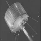
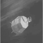
validation images

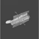
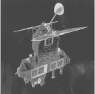
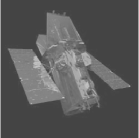
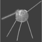
Figure 1. Four prototype true images used for generating the training set (top row) and validation set (bottom row) in the OID experiment with ${\bm{\theta}}=[\lambda,p,q]^{\top}$.

For the forward model, we consider a blurring process defined by an isotropic Gaussian blur centered at location $(\chi_{1},\chi_{2})$, where the point spread function ${\bf P}$ has entries

$$[P]_{i,j}={c(\sigma_{1},\sigma_{2})}\exp\left(-\frac{(i-\chi_{1})^{2}}{2\sigma_{1}^{2}}-\frac{(j-\chi_{2})^{2}}{2\sigma_{2}^{2}}\right)\,,$$ (20)

where $c(\sigma_{1},\sigma_{2})$ is a scaling factor. In the following we use the notation ${\bf A}={\bf A}(\sigma_{1},\sigma_{2})$ to highlight the dependence of the matrix ${\bf A}$ on the blurring parameters, and we consider periodic boundary conditions.

The observed image is obtained as in (1), with ${\bf A}(2.5,2.5)$ and ${\bf e}$ being impulse noise, with noise level selected uniformly at random between 10% and 50%. More specifically impulse noise is obtained when the entries of the vector ${\bf b}$ are constructed as follows

$${\bf b}_{i}=\left\{\begin{array}[]{ll}({\bf A}{\bf x}_{\rm true})_{i}&\mbox{with probability $1-\eta$,}\\ u_{i}&\mbox{with probability $\eta$,}\end{array}\right.$$

where $0\leq\eta<1$ denotes the (relative) noise level and $u_{i}$ is a number chosen randomly in the range of values of ${\bf A}{\bf x}_{\rm true}$. Although the images were generated using ${\bf A}(2.5,2.5)$, we consider reconstruction methods that use a different model matrix ${\bf A}(2.5,3.2)$, i.e., we introduce errors in the Gaussian blur parameters to model the realistic situation where the forward operator contains uncertainty and does not match data from the actual model. We are interested in computing a value of $p$ such that the fit-to-data ${\rm L}^{p}$ norm in (8b) is suitable for handling the model mismatch.

Using the OID approaches described in Section 3.1 with MM-GKS solvers for the inner problem, we compute the following optimal parameters.

• First, for fixed $p$ and $q$ we learn $\lambda$ only. For example, we denote ‘OID_λ,2,2’ as OID with $\theta=\lambda$ and $p=q=2$, and we denote ‘OID_λ,1,2’ as OID with $\theta=\lambda$, $p=1$, and $q=2$. The value of the regularization parameters so obtained are $0.4040$ and $0.4005$, respectively.

• Then we learn the regularization parameter, fit-to-data norm, and regularization norm triplet. We refer to this approach as ‘OID_λ,p,q’ and we obtained the values of $\widehat{\bm{\theta}}=[\ \widehat{\lambda},\ \widehat{p},\ \widehat{q}\ ]^{\top}=[0.3427,0.8129,0.4795]^{\top}$.

All OID approaches use surrogate optimization with a maximum of $200$ iterations and with lower and upper bounds of $10^{-8}\leq\lambda\leq 10$ for OID_λ,2,2 and OID_λ,1,2, and lower and upper bounds of $10^{-8}\leq\lambda\leq 10$, $0.1\leq p,q\leq 2.5$ for OID_λ,p,q. For the inner problem, we prescribed $50$ iterations of MM-GKS and $100$ iterations of CGLS (for $p=q=2$) at both training and validation stages. For all of the results in this section, we use the sample mean to center the data, prior to learning.

Using OID computed parameters, we obtain reconstructions for each of the validation images. In Figure 2 we provide the RRE norms for OID_λ,p,q (marked by yellow stars) for each validation image, where the index for the validation set has been sorted based on the RRE norms for OID_λ,p,q. RRE norms for OID_λ,2,2 (blue dots) and OID_λ,1,2 (red dots) are also provided for each validation image. Since most of the blue and red dots lie above the yellow stars, we conclude that OID_λ,p,q consistently performs better than OID_λ,2,2 and OID_λ,1,2, as expected. We also notice that RREs for OID_λ,2,2 are often smaller than RREs for OID_λ,1,2. Nevertheless, we observe that OID_λ,1,2 reconstructions eliminate the impulse noise well while struggling mitigate model errors in comparison to OID_λ,2,2 reconstructions, see Figure 3 (bottom left and middle).

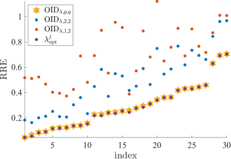
Figure 2. For the image deblurring problem with model error and impulse noise, we provide scatter plots of RRE norms for OID_λ,p,q, OID_λ,2,2 and OID_λ,1,2. Each column of dots corresponds to one sample from the validation set, where the indices have been sorted based on the RRE norms for OID_λ,p,q. As a further comparison, $\lambda_{\rm opt}^{j}$ corresponds to RRE norms for (21), where the optimal regularization parameter is selected for each image using the learned $\widehat{p}$ and $\widehat{q}$.

To investigate the impact of the regularization parameter $\lambda$, we also provide results for the OID${}_{\lambda,\widehat{p},\widehat{q}}$ method, i.e., OID where the previously computed values for $p$ and $q$ are fixed. Namely, the optimal regularization parameter $\lambda_{\rm opt}^{j}$ is computed for each validation image as

$$\begin{gathered}\lambda_{\rm opt}^{j}=\operatorname*{arg\,min}_{\lambda}\;\tfrac{1}{2}\left\|\widehat{\bf x}^{j}(\lambda)-{\bf x}_{\rm true}^{j}\right\|_{2}^{2}\,,\\ \text{ where }\;\widehat{{\bf x}}^{j}(\lambda)=\operatorname*{arg\,min}_{{\bf x}}\ \left\|{\bf A}{\bf x}-{\bf b}^{j}\right\|_{\widehat{p}}^{\widehat{p}}+\lambda\left\|{\bf x}\right\|_{\widehat{q}}^{\widehat{q}}\,,\end{gathered}$$ (21)

with the OID_λ,p,q computed values $\widehat{p}=0.8129$, $\widehat{q}=0.4795$. RRE values for each validation image are provided as purple dots in Figure 2. As expected, the images reconstructed using the optimal regularization parameter for each validation image have smaller RRE values than the images reconstructed using OID_λ,p,q parameters. However, we stress that this approach is not feasible in practice and that the OID results are not far off. Reconstructed images along with RRE values for one validation image are provided in Figure 3. We observe that the OID_λ,p,q reconstruction does not contain artifacts that are present in the OID_λ,2,2 and OID_λ,1,2 reconstructions (due to the learning of $p$ and $q$), and the reconstruction with the optimal regularization parameter is only slightly better and nearly indistinguishable from the OID_λ,p,q reconstruction.

${\bf x}_{\rm true}$	${\bf b}$ (RRE = 0.4402)	OIDλ,p,q (RRE = 0.1238)
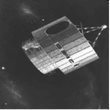
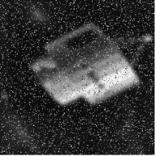
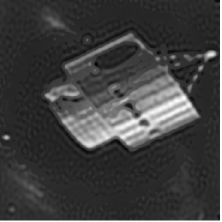
OIDλ,2,2 (RRE = 0.2064)	OIDλ,1,2 (RRE = 0.3728)	${\lambda_{\rm opt}^{j}}$ (RRE = 0.1235)

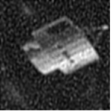
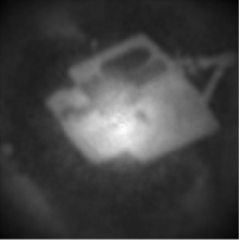
Figure 3. For one sample of the validation data set, we provide in the top row the true image, the observed image, and the OID_λ,p,q reconstruction. In the bottom row are reconstructions for OID_λ,2,2 and OID_λ,1,2. The bottom right reconstruction was computed using the optimal regularization parameter for this image and is provided for comparison purposes only. RRE values are provided in the titles.

We remark that we observed similar performance for an example where the amount of blur is underestimated at the reconstruction stage; that is, training and validation data were generated using ${\bf A}(2.5,3.2),$ but ${\bf A}(2.5,2.5)$ was used for reconstructions. However, we do not provide results here.

Next, we investigate the impact of model error on the noise and hence the data-fit term, for which it is well-known that the choice of $p$ is directly related to the statistics of the observation error. For one satellite image ${\bf x}_{\rm true}$, we consider the observed image that is generated using ${\bf A}(2.5,2.5)$ and we consider observation errors coming from two sources: 1% additive Gaussian noise and model error by using ${\bf A}(5.6,5.6)$ for reconstructions instead of ${\bf A}(2.5,2.5)$. Images of the additive Gaussian noise, the model error, i.e., ${\bf A}(5.6,5.6){\bf x}_{\rm true}-{\bf A}(2.5,2.5){\bf x}_{\rm true}$, and the sum of the two sources of errors are provided in the top row of Figure 4 from left to right. These represent pixel-wise quantities. In the lower frame, we provide a density plot of the combined error, along with the density functions corresponding to $p=2$ and $p=1.3835$ (the best $p$-norm density fit for this image).

${\bf A}(2.5,2.5){\bf x}_{\rm true}-{\bf b}$	$({\bf A}(5.6,5.6)-{\bf A}(2.5,2.5)){\bf x}_{\rm true}$	${\bf A}(5.6,5.6){\bf x}_{\rm true}-{\bf b}$

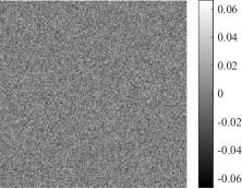
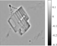
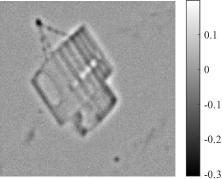
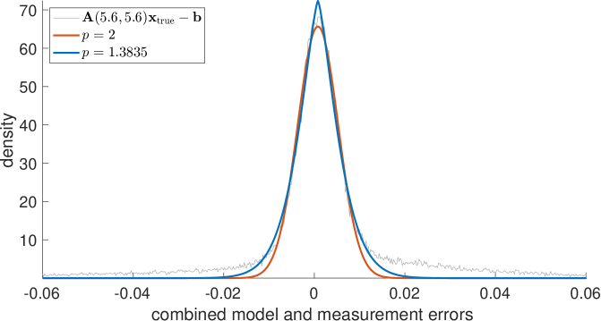
Figure 4. Investigating the impact of model error on the overall noise statistics. From left to right in the top row, we provide pixel-wise values of the additive Gaussian noise (of level 1%), the model error, and the sum of these two errors. The density plot for the combined error is provided, along with the density function for $p=2$ (corresponding to Gaussian noise) and the best density fit to the true errors ${\bf A}(5.6,5.6){\bf x}_{\rm true}-{\bf b}$, i.e., $p=1.3835$.

We observe that the combined model and measurement error, which resembles a heavy-tailed distribution, results in a noise distribution that is no longer Gaussian (i.e., ignoring the model error and using $p=2$ may not be appropriate). Indeed, even with additive Gaussian noise, there exists a value for $p$ that better resembles the noise statistics when model error is present. Thus, without additional prior knowledge, changing the norm for the data-fit term (in effect learning the statistics of the combined additive and model error from training data) is a reasonable approach to handle model error.

4.2. OID for learning kernel parameter(s) and regularization parameter

We consider a seismic imaging problem (namely, PRseismic from [37]) that can be modeled as (1), with ${\bf x}_{\rm true}$ containing a smooth image; see Figure 5. ${\bf A}$ represents 2D seismic travel-time tomography, using $n_{\rm s}=256$ sources located on the right boundary and $n_{\rm r}=512$ receivers (seismographs) scattered along the left and top boundaries. The rays are transmitted from each source to each receiver. The noisy observations are provided in Figure 5; here $n=65,\!536=256^{2}$.

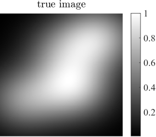
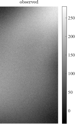
Figure 5. Seismic image reconstruction example. The true image (left) contains $256\times 256$ pixels and represents a smooth medium. The noisy sinogram image (right) represents projection data from a setup with $256$ sources and $512$ receivers.

We generated a set of $30$ training images, some samples are provided in Figure 6. These were obtained by randomizing the parameters used to define the “smooth” image in IRTools [29]. Then for each training image, we simulated noisy observations using realizations of a Gaussian random vector with ${\bf 0}$ mean and noise level $\eta=\frac{\|{\bf e}\|_{2}}{\|{\bf A}{\bf x}_{\rm true}\|_{2}}$ uniformly chosen between $10^{-2}$ and $10^{-1}$.

Using the training data, we consider two kernel functions, the squared exponential kernel function (17) and the Mat$\acute{\text{e}}$rn kernel function (18). For each kernel function, we provide OID results for the following two scenarios:

• ‘OID’ corresponds to solving (8) with ${\bm{\theta}}=[\lambda,{\bm{\beta}}]$, where the genGK-based iterative projection method described in Section 3.2 is used to solve the inner problem (8b). Here we note that, since $\lambda$ is being learned in the OID problem, the only stopping criteria used for the inner problem are based on tolerances on the residual norm.

• OID with ${\bm{\theta}}={\bm{\beta}}$, where genHyBR is used for selecting $\lambda$ according to WGCV (weighted generalized cross validation) and the full suite of stopping criteria are used within genHyBR. We refer to this approach as ‘OID-wgcv’.

Both OID approaches use surrogate optimization with a maximum of $20$ iterations and with lower and upper bounds of $10^{-6}\leq\lambda\leq 1$, $0.5\leq\beta_{1}\leq 15$, and $5\cdot 10^{-2}\leq\beta_{2}\leq 0.7$ for the Mat$\acute{\text{e}}$rn kernel and $10^{-6}\leq\lambda\leq 1$ and $0.01\leq\beta\leq 0.5$ for the squared exponential kernel. Computed OID parameters are given in Table 1.

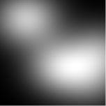
Figure 6. Seismic example - random samples from the training set

Then similar to how we generated the training images, we generated $100$ validation images and their corresponding observations. Using the OID parameters in Table 1, we obtained reconstructions for the validation set. The overall mean squared reconstruction error for the validation images is provided in the last column of Table 1. Individually computed RRE norms for OID and OID-wgcv for each validation image are provided as yellow and red dots in Figure 8 respectively, where the indices have been sorted based on the RRE norms for OID. Notice that most of the red dots lie above the yellow dots, and thus OID tends to perform better than OID-wgcv for this example.

For comparison, we use the approach described in [17] that estimates hyperparameters directly from the the sample covariance matrix constructed from the training data, followed by genHyBR with WGCV for selecting $\lambda$. Following [17], let $\widehat{\bf Q}$ be the sample covariance matrix constructed from the training dataset, then Mat$\acute{\text{e}}$rn parameters were estimated by solving

$$(\hat{\nu},\hat{\ell})=\operatorname*{arg\,min}_{\nu>0,\ell>0}\left\|{\bf Q}(\nu,\ell)-\widehat{\bf Q}\right\|_{\rm F}^{2},$$ (22)

where $\left\|\,\cdot\,\right\|_{{\rm F}}$ denotes the Frobenius norm. Once the parameters are computed, they can be used to define ${\bf Q}={\bf Q}(\hat{\nu},\hat{\ell})$, which can be used directly in generalized hybrid methods. For computational feasibility, a stochastic approximation is used for the objective function in (22), i.e.,

$$\left\|{\bf Q}(\nu,\ell)-\widehat{{\bf Q}}\right\|_{{\rm F}}^{2} =\mathbb{E}\left\|({\bf Q}(\nu,\ell)-\widehat{{\bf Q}}){\bm{\xi}}\right\|_{2}^{2},$$ (23)

where ${\bm{\xi}}$ is a random variable such that $\mathbb{E}{\bm{\xi}}={\bf 0}$ and $\mathbb{E}({\bm{\xi}}{\bm{\xi}}^{\top})={\bf I}$. Using a Hutchinson trace estimator, we let ${\bm{\xi}}^{(i)}\in\mathbb{R}^{n}$ for $i=1,2,\ldots,M$ be realizations of a Rademacher distribution (i.e., ${\bm{\xi}}$ consists of $\pm 1$ with equal probability), and we consider the approximate optimization problem,

$$(\check{\nu},\check{\ell})=\operatorname*{arg\,min}_{\nu>0,\ell>0}\frac{1}{M}\sum_{i=1}^{M}\|({\bf Q}(\nu,\ell)-\widehat{\bf Q}){\bm{\xi}}^{(i)}\|^{2}_{2}\,.$$ (24)

Similar to the approach described in [17], we used an interior-point method (fmincon.m in MATLAB) to minimize (24) with $M=100$, and refer to this approach as sample covariance (SC). We extend this approach to be used for estimating the squared exponential kernel parameter $\beta$ and provide the computed hyperparameters in the row labeled ‘SC’ in Table 1. We remark that this approach uses only the training data and not the model, noise or observations for learning the kernel parameter. On the contrary, OID incorporates this information. Also, for comparison, we provide results for standard Tikhonov regularization (${\bf Q}={\bf I}$) with the optimal $\lambda$ selected for each sample. The goal of this comparison is to show that including the prior is critical for this example. Scatter plots of RRE values for both approaches are provided in Figure 7. Density graphs of the reconstruction errors are provided in Figure 8, and one reconstructed image is provided in Figure 9.

Mat$\acute{\text{e}}$rn	$\lambda$	${\bm{\beta}}$	$\mathcal{P}$, validation
OID	18.8313	5.0312, 0.3344	6.0833
OID	wgcv	12.2812, 0.3344	29.9412
SC	wgcv	123.1735, 0.2011	49.3447
sq. exp.	$\lambda$	$\beta$	$\mathcal{P}$, validation
OID	50.0500	0.2550	3.4468
OID	wgcv	0.3163	24.7547
SC	wgcv	0.2010	47.6977

Table 1. Computed values of the hyperparameters for OID, along with the mean reconstruction errors for the validation set. OID with $\lambda$ computed using WGCV corresponds to using OID-wgcv for estimating ${\bm{\beta}}$ only. ‘SC’ corresponds to estimating ${\bm{\beta}}$ directly from the sample covariance matrix as described in [17] and then using genHyBR with WGCV.

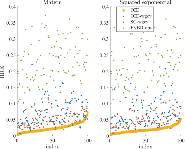
Figure 7. For the seismic example, we provide scatter plots of RRE norms for OID, OID-wgcv, SC-wgcv, and HyBR opt. Each column of dots corresponds to one sample from the validation set, where the indices have been sorted based on the RRE norms for OID.

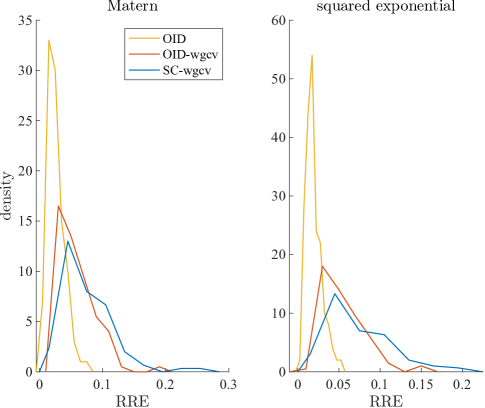
Figure 8. For the validation set of the seismic example, we provide histograms of the RRE norms for OID, OID-wgcv, and SC-wgcv.

$\lambda_{\rm opt}$ ${\bf Q}={\bf I}$	OID Mat$\acute{\text{e}}$rn	OID sq. exp.
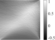
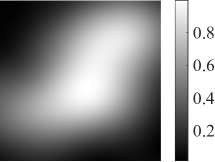
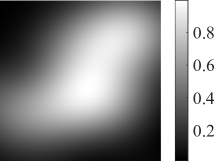
(RRE = 0.2554)	(RRE = 0.0214)	(RRE = 0.0190)

Figure 9. For the validation image in Figure 5, we provide reconstructions obtained with HyBR opt and OID reconstructions for the Mat$\acute{\text{e}}$rn and squared exponential kernels.

Finally, we investigate the properties of the design objective function (8a) for OID with the squared exponential kernel. In Figure 10, we provide a contour plot of the design objective function, where the white point corresponds to the OID computed values. Notice that there is wide region of values for $\lambda$ and $\beta$ that result in small and similar design objective values, with a smaller range of good choices for $\beta$.

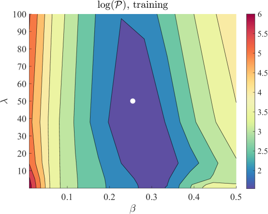
Figure 10. Design objective for OID with the squared exponential kernel for the seismic example. The filled contour corresponds to OID, and the white point denotes the OID computed values.

5. Conclusions and extensions

In this work, we have presented a unified framework for optimal inversion design for large-scale inverse problems. We have described learning approaches for computing hyperparameters from training data that exploit Krylov subspace methods for efficiently solving regularized inner problems within bi-level schema. In particular, we considered OID for learning the norm exponent in the data-fit and regularization term, as well as for learning the regularization parameter. Furthermore, we considered OID for learning parameters for kernel functions used to define prior covariance matrices. Numerical experiments showed that OID methods can compute hyperparameters that deliver quality reconstructions, even in especially relevant scenarios where there is a mixture of noise and model error in the data (e.g., due to the presence of inaccuracies in the forward operator).

We remark that there are other cases where data-driven, optimal inverse frameworks can be used. The focus of our applications is image processing, and more particularly, image deblurring and computerized tomography; nevertheless, the learning approaches that we propose here can be applied to broad applications outside the field of image processing. Moreover, general regularization matrices can be used when considering OID with ${\bm{\theta}}=[p,q,\lambda]^{\top}$, including: discretizations of the derivative operators when solutions with edge preserving properties are desired, wavelet and framelet transformations like in [9, 10, 11, 12, 42] when the solution is sparse in a transformed domain, or fractional Laplacian regularizers where smoothness is determined by a fractional exponent [2]. Other extensions include more general model errors, e.g., where the true forward model is a matrix perturbation of the forward model matrix, and stochastic approximation methods for problems where the training set is very large and hence empirical Bayes risk minimization problems become computationally intractable. These are topics of future investigations.

References

- [1] Alen Alexanderian, Philip J Gloor and Omar Ghattas “On Bayesian A-and D-optimal experimental designs in infinite dimensions” In Bayesian Analysis 11.3 International Society for Bayesian Analysis, 2016, pp. 671–695
- [2] Harbir Antil, Zichao Wendy Di and Ratna Khatri “Bilevel optimization, deep learning and fractional Laplacian regularization with applications in tomography” In Inverse Problems 36.6 IOP Publishing, 2020, pp. 064001
- [3] Francesco Archetti and Antonio Candelieri “The Acquisition Function” In Bayesian Optimization and Data Science Springer, 2019, pp. 57–72
- [4] Simon Arridge, Peter Maass, Ozan Öktem and Carola-Bibiane Schönlieb “Solving inverse problems using data-driven models” In Acta Numerica 28 Cambridge University Press, 2019, pp. 1–174
- [5] Anthony Curtis Atkinson and Alexander N Donev “Optimum Experimental Designs”, 1992
- [6] Johnathan M Bardsley and James G Nagy “Covariance-preconditioned iterative methods for nonnegatively constrained astronomical imaging” In SIAM Journal on Matrix Analysis and Applications 27.4 SIAM, 2006, pp. 1184–1197
- [7] A. Björk “Numerical Methods for Least Squares Problems” SIAM, 1996
- [8] Richard D Brown, Johnathan M Bardsley and Tiangang Cui “Semivariogram methods for modeling Whittle–Matérn priors in Bayesian inverse problems” In Inverse Problems 36.5 IOP Publishing, 2020, pp. 055006
- [9] A Buccini, M Pasha and L Reichel “Modulus-based iterative methods for constrained minimization” In Inverse Problems 36.8 IOP Publishing, 2020, pp. 084001
- [10] Alessandro Buccini, Yonggi Park and Lothar Reichel “Numerical aspects of the nonstationary modified linearized Bregman algorithm” In Applied Mathematics and Computation 337 Elsevier, 2018, pp. 386–398
- [11] Alessandro Buccini, Mirjeta Pasha and Lothar Reichel “Projected Bregman in Krylov Subspaces.” In Mathematics of Computation 78.267, 2009, pp. 1515–1536
- [12] Jian-Feng Cai, Stanley Osher and Zuowei Shen “Linearized Bregman iterations for frame-based image deblurring” In SIAM Journal on Imaging Sciences 2 SIAM, 2009, pp. 226–252
- [13] Luca Calatroni, Juan Carlos De Los Reyes and Carola-Bibiane Schönlieb “Infimal convolution of data discrepancies for mixed noise removal” In SIAM Journal on Imaging Sciences 10.3 SIAM, 2017, pp. 1196–1233
- [14] Luca Calatroni et al. “Bilevel approaches for learning of variational imaging models” In Variational Methods: In Imaging and Geometric Control 18.252 Walter de Gruyter GmbH, 2017, pp. 2
- [15] D. Calvetti and E. Somersalo “An Introduction to Bayesian Scientific Computing: Ten Lectures on Subjective Computing” Springer Science & Business Media, 2007
- [16] Antonin Chambolle and Thomas Pock “A first-order primal-dual algorithm for convex problems with applications to imaging” In Journal of Mathematical Imaging and Vision 40.1 Springer, 2011, pp. 120–145
- [17] Taewon Cho, Julianne Chung and Jiahua Jiang “Hybrid projection methods for large-scale inverse problems with mixed Gaussian priors” In Inverse Problems 37.4 IOP Publishing, 2021, pp. 044002
- [18] J. Chung and S. Gazzola “Flexible Krylov Methods for Regularization” In SIAM Journal on Scientific Computing 41.5 SIAM, 2019, pp. S149–S171
- [19] Julianne Chung, Matthias Chung and Dianne P O’Leary “Designing optimal spectral filters for inverse problems” In SIAM Journal on Scientific Computing 33.6 SIAM, 2011, pp. 3132–3152
- [20] Julianne Chung and Malena I Español “Learning regularization parameters for general-form Tikhonov” In Inverse Problems 33.7 IOP Publishing, 2017, pp. 074004
- [21] Julianne Chung and James G Nagy “An efficient iterative approach for large-scale separable nonlinear inverse problems” In SIAM Journal on Scientific Computing 31.6 SIAM, 2010, pp. 4654–4674
- [22] Julianne Chung and Arvind K Saibaba “Generalized hybrid iterative methods for large-scale Bayesian inverse problems” In SIAM Journal on Scientific Computing 39.5 SIAM, 2017, pp. S24–S46
- [23] Juan Carlos De los Reyes, C-B Schönlieb and Tuomo Valkonen “Bilevel parameter learning for higher-order total variation regularisation models” In Journal of Mathematical Imaging and Vision 57.1 Springer, 2017, pp. 1–25
- [24] Juan Carlos De los Reyes and Carola-Bibiane Schönlieb “Image denoising: learning the noise model via nonsmooth PDE-constrained optimization.” In Inverse Problems & Imaging 7.4, 2013
- [25] Stephan Dempe “Foundations of Bilevel Programming” Springer Science & Business Media, 2002
- [26] Matthew M Dunlop, Tapio Helin and Andrew M Stuart “Hyperparameter Estimation in Bayesian MAP Estimation: Parameterizations and Consistency” In arXiv preprint arXiv:1905.04365, 2019
- [27] Heinz Werner Engl, Martin Hanke and Andreas Neubauer “Regularization of Inverse Problems” Springer Science & Business Media, 1996
- [28] Ernie Esser, Xiaoqun Zhang and Tony F Chan “A general framework for a class of first order primal-dual algorithms for convex optimization in imaging science” In SIAM Journal on Imaging Sciences 3.4 SIAM, 2010, pp. 1015–1046
- [29] Silvia Gazzola, Per Christian Hansen and James G Nagy “IR Tools: a MATLAB package of iterative regularization methods and large-scale test problems” In Numerical Algorithms 81.3 Springer, 2019, pp. 773–811
- [30] “Global Optimization Toolbox” Accessed: 2021-09-20, https://www.mathworks.com/help/gads/index.html?s_tid=CRUX_lftnav
- [31] Robert B Gramacy “Surrogates: Gaussian process modeling, design, and optimization for the applied sciences” ChapmanHall/CRC, 2020
- [32] E Haber and L Tenorio “Learning regularization functionals—a supervised training approach” In Inverse Problems 19.3 IOP Publishing, 2003, pp. 611
- [33] Eldad Haber, Lior Horesh and Luis Tenorio “Numerical methods for experimental design of large-scale linear ill-posed inverse problems” In Inverse Problems 24.5 IOP Publishing, 2008, pp. 055012
- [34] Eldad Haber, Lior Horesh and Luis Tenorio “Numerical methods for the design of large-scale nonlinear discrete ill-posed inverse problems” In Inverse Problems 26.2 IOP Publishing, 2010, pp. 025002
- [35] Markus Haltmeier and Linh V Nguyen “Regularization of Inverse Problems by Neural Networks” In arXiv preprint arXiv:2006.03972, 2020
- [36] Kerstin Hammernik et al. “Learning a variational network for reconstruction of accelerated MRI data” In Magnetic Resonance in Medicine 79.6 Wiley Online Library, 2018, pp. 3055–3071
- [37] Per Christian Hansen and Jakob Sauer Jørgensen “AIR Tools II: algebraic iterative reconstruction methods, improved implementation” In Numerical Algorithms 79.1 Springer, 2018, pp. 107–137
- [38] Michael Hintermüller, Carlos N Rautenberg, Tao Wu and Andreas Langer “Optimal selection of the regularization function in a weighted total variation model. Part II: Algorithm, its analysis and numerical tests” In Journal of Mathematical Imaging and Vision 59.3 Springer, 2017, pp. 515–533
- [39] Gernot Holler, Karl Kunisch and Richard C Barnard “A bilevel approach for parameter learning in inverse problems” In Inverse Problems 34.11 IOP Publishing, 2018, pp. 115012
- [40] Xun Huan and Youssef Marzouk “Gradient-based stochastic optimization methods in Bayesian experimental design” In International Journal for Uncertainty Quantification 4.6 Begel House Inc., 2014
- [41] G Huang et al. “Majorization–minimization generalized Krylov subspace methods for optimization applied to image restoration” In BIT Numerical Mathematics 57.2 Springer, 2017, pp. 351–378
- [42] Jie Huang, Marco Donatelli and Raymond H Chan “Nonstationary iterated thresholding algorithms for image deblurring.” In Inverse Problems & Imaging 7, 2013, pp. 717–736
- [43] David R Hunter and Kenneth Lange “A tutorial on MM algorithms” In The American Statistician 58.1 Taylor & Francis, 2004, pp. 30–37
- [44] Jari Kaipio and Erkki Somersalo “Statistical and Computational Inverse Problems” Springer Science & Business Media, 2006
- [45] Jari P Kaipio, Ville Kolehmainen, Marko Vauhkonen and Erkki Somersalo “Inverse problems with structural prior information” In Inverse problems 15.3 IOP Publishing, 1999, pp. 713
- [46] Marie Kubínová and James G Nagy “Robust regression for mixed Poisson–Gaussian model” In Numerical Algorithms 79.3 Springer, 2018, pp. 825–851
- [47] Kenneth Lange “MM optimization algorithms” SIAM, 2016
- [48] Housen Li, Johannes Schwab, Stephan Antholzer and Markus Haltmeier “NETT: Solving inverse problems with deep neural networks” In Inverse Problems IOP Publishing, 2020
- [49] Alice Lucas, Michael Iliadis, Rafael Molina and Aggelos K Katsaggelos “Using deep neural networks for inverse problems in imaging: beyond analytical methods” In IEEE Signal Processing Magazine 35.1 IEEE, 2018, pp. 20–36
- [50] Sebastian Lunz, Ozan Öktem and Carola-Bibiane Schönlieb “Adversarial regularizers in inverse problems” In Advances in Neural Information Processing Systems 31, 2018, pp. 8507–8516
- [51] Sebastian Lunz et al. “On learned operator correction in inverse problems” In SIAM Journal on Imaging Sciences 14.1 SIAM, 2021, pp. 92–127
- [52] Michael T McCann, Kyong Hwan Jin and Michael Unser “Convolutional neural networks for inverse problems in imaging: A review” In IEEE Signal Processing Magazine 34.6 IEEE, 2017, pp. 85–95
- [53] “NASA”, http:www.nasa.gov
- [54] Gregory Ongie et al. “Deep learning techniques for inverse problems in imaging” In IEEE Journal on Selected Areas in Information Theory IEEE, 2020
- [55] Michael A Osborne, Roman Garnett and Stephen J Roberts “Gaussian processes for global optimization” In 3rd international conference on learning and intelligent optimization (LION3), 2009, pp. 1–15
- [56] P.. “Discrete Inverse Problems: Insight and Algorithms” SIAM, 2010
- [57] Jean Prost, Antoine Houdard, Andrés Almansa and Nicolas Papadakis “Learning local regularization for variational image restoration” In arXiv preprint arXiv:2102.06155, 2021
- [58] Friedrich Pukelsheim “Optimal design of experiments” SIAM, 2006
- [59] Nicolai André Brogaard Riis, Yiqiu Dong and Per Christian Hansen “Computed tomography with view angle estimation using uncertainty quantification” In Inverse Problems 37.6 IOP Publishing, 2021, pp. 065007
- [60] Lars Ruthotto, Julianne Chung and Matthias Chung “Optimal experimental design for inverse problems with state constraints” In SIAM Journal on Scientific Computing 40.4 SIAM, 2018, pp. B1080–B1100
- [61] Ferdia Sherry et al. “Learning the sampling pattern for MRI” In IEEE Transactions on Medical Imaging IEEE, 2020
- [62] Ankur Sinha, Pekka Malo and Kalyanmoy Deb “A review on bilevel optimization: from classical to evolutionary approaches and applications” In IEEE Transactions on Evolutionary Computation 22.2 IEEE, 2017, pp. 276–295
- [63] Danny Smyl et al. “Learning and correcting non-Gaussian model errors” In Journal of Computational Physics 432 Elsevier, 2021, pp. 110152
- [64] Magnus Urquhart, Emil Ljungskog and Simone Sebben “Surrogate-based optimisation using adaptively scaled radial basis functions” In Applied Soft Computing 88 Elsevier, 2020, pp. 106050
- [65] Thomas Weise “Global optimization algorithms-theory and application” In Self-Published Thomas Weise, 2009
- [66] Christopher K Williams “Gaussian processes for machine learning” MIT Press, 2006
- [67] Kai Zhang, Wangmeng Zuo, Shuhang Gu and Lei Zhang “Learning deep CNN denoiser prior for image restoration” In Proceedings of the IEEE conference on computer vision and pattern recognition, 2017, pp. 3929–3938
- [68] Mingqiang Zhu and Tony Chan “An efficient primal-dual hybrid gradient algorithm for total variation image restoration” In UCLA CAM Report 34 Citeseer, 2008, pp. 8–34