Generalizing Neural Networks by Reflecting Deviating Data in Production

Abstract.

Trained with a sufficiently large training and testing dataset, Deep Neural Networks (DNNs) are expected to generalize. However, inputs may deviate from the training dataset distribution in real deployments. This is a fundamental issue with using a finite dataset. Even worse, real inputs may change over time from the expected distribution. Taken together, these issues may lead deployed DNNs to mis-predict in production.

In this work, we present a runtime approach that mitigates DNN mis-predictions caused by the unexpected runtime inputs to the DNN. In contrast to previous work that considers the structure and parameters of the DNN itself, our approach treats the DNN as a blackbox and focuses on the inputs to the DNN. Our approach has two steps. First, it recognizes and distinguishes “unseen” semantically-preserving inputs. For this we use a distribution analyzer based on the distance metric learned by a Siamese network. Second, our approach transforms those unexpected inputs into inputs from the training set that are identified as having similar semantics. We call this process input reflection and formulate it as a search problem over the embedding space on the training set. This embedding space is learned by a Quadruplet network as an auxiliary model for the subject model to improve the generalization.

We implemented a tool called InputReflector based on the above two-step approach and evaluated it with experiments on three DNN models trained on CIFAR-10, MNIST, and FMINST image datasets. The results show that InputReflector can effectively distinguish inputs that retain semantics of the distribution (e.g., blurred, brightened, contrasted, and zoomed images) and out-of-distribution inputs from normal inputs.

1. Introduction

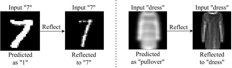
Figure 1. Input reflection examples.

Deep Neural Networks (DNNs) have achieved high performance across many domains, notably in classification tasks, such as object detection (Redmon et al., 2016), image classification (He et al., 2016), medical diagnostics (Ciresan et al., 2012), and semantic segmentation (Long et al., 2015). Today, these DNNs are trained on large amounts of data and then deployed for real-world use.

DNNs require that inputs in deployment come from the same distribution as the training dataset. However, real world inputs that are semantically similar to a human observer may look different from the perspective of the model. For example, the distribution of data observed by an onboard camera of a self-driving car may change due to environmental factors; the images may be brighter or more blurry than those in the training dataset. Even worse, altogether new and unexpected inputs may be presented to a deployed model. When presented with such unexpected inputs, the model may manifest unexpected behaviors. For example, a model trained on MNIST (LeCun et al., 2010) may incorrectly classify a blurry digit.

The academic community and AI industry have proposed a variety of techniques to train an offline robust and trustworthy model, including data augmentation (Gao et al., 2020; Samangouei et al., 2018; Zhong et al., 2020; Dreossi et al., 2018), adversarial training (Ganin et al., 2016; Miyato et al., 2016; Shafahi et al., 2019; Shrivastava et al., 2017), and adversarial sample defense techniques (Samangouei et al., 2018; Ilyas et al., 2019; Wang et al., 2019a; Wang et al., 2019b; Zhang et al., 2020). All of these techniques aim to increase the range of the training dataset so that the trained model can better generalize. However, this generalization is ultimately constrained by the model architecture and the finite training dataset. The challenge is that real-world inputs in deployment can have unexpected variations, and these inputs may be difficult to capture through data augmentation during the training stage. One reason for this is that data enrichment-based techniques rely on a priori knowledge of the transformations that may appear in deployment. Furthermore, such solutions may sacrifice accuracy to improve generalization ability. Recent work considers online retraining/learning approaches (Gao et al., 2021), but these have a high performance cost and may not be appropriate for applications with timing constraints.

For out-of-distribution inputs a variety of techniques exist, including ODIN (Liang et al., 2018), Mahalanobis (LEE et al., 2018), and Generalized ODIN (Hsu et al., 2020). These techniques distinguish out-of-distribution from in-distribution data. But, none of them focuses on identifying deviating data with similar semantics to the training data. That is, they do not distinguish inputs that are further away from the training dataset but closer than out-of-distribution data.

We present a runtime input-reflection approach that (1) recognizes “unseen” semantic-preserving inputs (e.g., bright or blurry images, text written by non-native speakers with grammatical deviations, dialect speech inputs) for a DNN model, and (2) reflects them to samples in the training dataset that conform to a similar distribution. This second step improves model generalization. The key insight of our approach is that an “unseen” input can be potentially mapped into a semantically similar “seen” input on which the model can make a more trustworthy decision.

Figure 1 presents two examples where the input reflection process corrects the classification of a brightened digit “7” and a blurry “dress”. The digit “7” presents a different handwriting style (e.g., with thicker strokes than those in the training data), causing the model to miss-predict it as a “1”. Our reflection approach , without learning any handwriting style, can reflect this input into a digit “7” from the training dataset to mitigate the miss-prediction. Similarly, the right side of Figure 1 shows a blurry “dress” input. The DNN model incorrectly classifies this input as a “pullover”. By contrast, the reflected version is correctly classified as a “dress”. Both examples illustrate how input reflection can help DNNs deal with unexpected inputs in production.

Realizing input reflection requires addressing two technical challenges. First, we need a technique to distinguish normal inputs (e.g., a digit from the MNIST dataset), semantically similar inputs unseen during training (e.g., a blurry or bright digit), and out-of-distribution inputs (e.g., a non-digit image). The second challenge is to design a reflection process to map inputs unseen during training into semantically similar inputs from the training dataset.

There are a variety of DNN models. In this work we make the first attempt to reflect inputs by overcoming the above challenges in the context of computer vision models. We leave other domains for future work. For challenge (1), we invent a measurement based on a Siamese network, which can discriminate the normal input, unseen deviated input, and out-of-distribution input. For challenge (2), we convert the reflection problem into a problem of finding similar inputs in the training dataset based on the learned embeddings by a Quadruplet network, which can capture the similarity of learned embedding from two images.

In summary, we make the following contributions:

• We propose a novel technique to improve DNN generalization by focusing on DNN inputs and treating the DNN as a black-box in production. Our technique contributes (1) a general discriminative measurement to distinguish normal, deviated, and out-of-distribution inputs; and (2) a search method to reflect an unexpected input into one that has similar semantics and is present in the training set.

• We implemented a tool called InputReflector based on the above approach, and evaluate it on three DNN models (ConvNet, VGG-16, and ResNet-20) trained on the CIFAR-10, MNIST, and FMNIST datasets. Our experimental results show that our tool InputReflector can recognize 77.19% of the deviated inputs and fix 77.50% of them. Our implementation is open-source.

2. Background

In this section we review Siamese networks and triplet loss, which are key to our solution.

2.1. Siamese Network

Bromley et al.(Bromley et al., 1993) introduced the idea of a Siamese network to quantify the similarity between two images. Their Siamese network quantifies the similarity between handwriting signatures. Typically, a Siamese network transforms the inputs x into a feature space $\textbf{z}=f(\textbf{x})$, where similar inputs have a shorter distance and dissimilar inputs have larger distance. Given a pair of inputs $\textbf{x}_{1}$ and $\textbf{x}_{2}$, we usually use Cosine similarity or Euclidean distance to compare $f(\textbf{x}_{1})$ and $f(\textbf{x}_{2})$. Siamese networks (Chicco, 2021) have been applied to a wide-range of applications, like object tracking (Zhang and Peng, 2019; Li et al., 2019), face recognition (Taigman et al., 2014), and image recognition (Koch et al., 2015). In this work, we use Siamese networks to evaluate the semantic similarity between an input in deployment and samples in the training dataset.

2.2. Triplet Loss

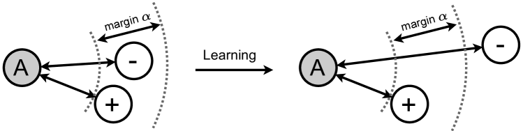
Figure 2. An example of using triplet loss.

Triplet loss was first proposed in FaceNet (Schroff et al., 2015). Given a training dataset where samples are labeled with classes, the triplet loss is designed to project the samples into a feature space where samples under the same class have shorter distance than those under different classes. Figure 2 shows an example of triplet loss. Given a sample as Anchor of class $c_{1}$, taking a positive sample (annotated as “+”) under $c_{1}$ and a negative sample (annotated as “-”) under $c_{2}$, triplet loss is designed to pull the positive sample closer while pushing the negative sample further from the anchor. Technically, the definition of triplet loss is as follows:

(1) $$\mathcal{L}_{\text{triplet}}=max(Dis(Anchor,Pos)-Dis(Anchor,Neg)+\alpha,0)$$

In the above, $\alpha$ is the margin, introduced to keep a distance gap between positive and negative samples. The loss can be optimized if the Siamese network can push $Dis(Anchor,Pos)$ to 0 and $Dis(Anchor,Neg)$ to be larger than $Dis(Anchor,Pos)+\alpha$.

Next, we describe our approach, which uses Siamese networks and triplet loss to realize input reflection.

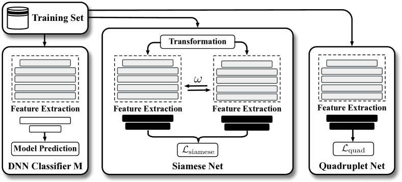
Figure 3. The design of InputReflector in training.

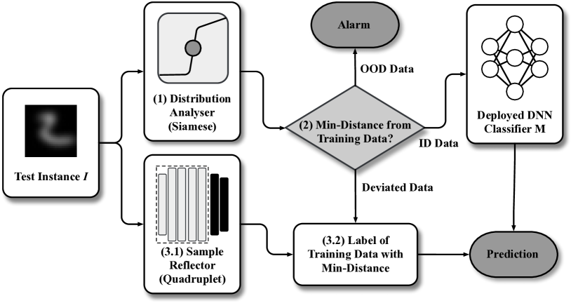
Figure 4. The design of InputReflector in deployment.

3. Design of InputReflector

Figure 3 and Figure 4 reviews the training-time and runtime design of InputReflector. We will refer to these figures in this section.

InputReflector uses information during model training to inform its runtime strategy. We review how InputReflector acquires the required information during training later in this section. At runtime, given an input $I$ and a deployed model $\mathit{M}$, InputReflector follows a three-step approach:

1. Determine if $\mathit{M}$ can correctly predict $I$ by checking how well $I$ conforms to the distribution of training dataset.

2. If $\mathit{M}$ cannot correctly predict $I$, then determine if $I$ shares similar semantics to the training samples.

3. If $I$ is semantically similar to the training samples, then determine which training sample is best used instead of $I$ for the prediction.

The key to the above steps is correct characterization of the semantics of an input. For this, we rely on sample distribution and design a Distribution Analyzer (Section 3.1). This piece of our approach is inspired by prior research (Qian et al., 2019; Kim et al., 2020) that indicates that the distribution of embedding vectors can be used to group semantically similar data (e.g., images of the same class). InputReflector uses the embedding distribution to check the semantic similarity between the test instance and the training data. For inputs that are classified by the Distribution Analyzer as deviating samples, we design the Sample Reflector (Section 3.2) to search for a close training sample to replace the runtime test instance.

We designed the Distribution Analyzer and Sample Reflector as auxiliary DNNs, for their inherent expressiveness. The Distribution Analyzer, implemented as a Siamese network, captures the general landscape of in-distribution, deviated, and out-of-distribution samples. The Sample Reflector, implemented as a Quadruplet network, calculates the detailed distance measurement between the samples.

Next, we detail the Distribution Analyzer and Sample Reflector.

3.1. Distribution Analyzer design

A challenge in building an effective Distribution Analyzer is designing a smooth measure for semantically same, similar, and dissimilar samples. Specifically, we need to design the auxiliary model so that samples can be projected into a space where there is such smoothness between the three categories.

To address this challenge, we require the auxiliary model to learn the smooth measurement from in-distribution, deviated, and out-of-distribution samples. Specifically, let an in-distribution sample be $x$, $K_{in}$ be the distance between $x$ and its most different semantic-preserving sample $x_{s}$, $K_{out}$ be the distance between $x$ and its most similar semantic-different sample $x_{o}$, any of semantic-preserving and deviating sample $x^{\prime}$ should conform to:

(2) $$K_{in}<min_{x_{t}\in\mathcal{X}^{t}}(f(x^{\prime},x^{t}))<K_{out}$$

To train a quality auxiliary model we prepare representative transformed samples that preserve the semantics of the training data. Specifically, our auxiliary models are trained on three types of data: (1) in-distribution samples (i.e., original training data), (2) deviating samples (i.e., representative transformed data), and (3) one kind of out-of-distribution samples (i.e., extremely transformed data, discussed in Section 4.1).

Next we discuss how we design the similarity function $f$ and how we generate $K_{in}$ and $K_{out}$.

3.1.1. Siamese Network Training

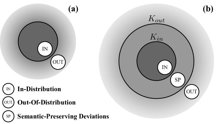
Figure 5. Comparison of problem formulation and thresholds used by (a) previous work, and (b) this paper.

Existing work on detecting out-of-distribution data uses one threshold Figure 5(a). By contrast, the challenge in our work is to find two thresholds, $K_{in}$ and $K_{out}$ in Figure 5(b), so that we can discriminate three types of data. Inspired by the Siamese network with triplet loss, which are used to identify people across cameras (Schroff et al., 2015; Chen et al., 2017), we build a Siamese network to learn two thresholds ($K_{in}$ and $K_{out}$) so that we can discriminate the three kinds of data.

To split the three kinds of data, both training data and their transformed versions are needed. For example, if we consider the blur transformation as an example, then the three kinds of data would be the normal training data $x$, blurry training data $x^{\prime}$, and very blurry training data $x^{\prime\prime}$ (Figure 3).

Our goal is to learn feature embeddings from the training dataset that push the semantic-preserving deviating input away from both the in-distribution data and out-of-distribution data. Specifically, the Siamese network in the distribution analyzer is designed to make the distance between the very blurry training data and the normal data larger than the distance between the blurry training data and the normal data. Formally, the aim of the Siamese network is $f(x_{c_{i}},x_{c_{j}})+K_{in}<f(x_{c_{i}},x^{{}^{\prime}}_{c})<f(x_{c_{i}},x_{c_{j}})+K_{out}<f(x_{c_{i}},x^{{}^{\prime\prime}}_{c})$. The loss function of this network is designed to minimize the objective:

(3) $$L= max(f(x_{c_{i}},x_{c_{j}})-f(x_{c_{i}},x^{{}^{\prime}}_{c})+m_{1},0)+$$

$$max(f(x_{c_{i}},x^{{}^{\prime}}_{c})-f(x_{c_{i}},x_{c_{j}})-m_{2},0)+$$

$$max(f(x_{c_{i}},x_{c_{j}})-f(x_{c_{i}},x^{{}^{\prime\prime}}_{c})+m_{2},0)$$

where $m_{1}$ and $m_{2}$ are the values of margins and $m_{1}<m_{2}$, $x_{c_{i}}$, $x_{c_{j}}$, and $x_{c}$ denote instances with the same label $c$ but $i\neq j$ which means that they are different instances.

This loss function consists of three components. The first and the last max components push both transformed versions of the training data away from the normal data but keep the extremely transformed version further away using a larger margin $m_{2}$. The middle max component is designed to distinguish transformed ($x^{\prime}$) and extremely transformed ones ($x^{\prime\prime}$).

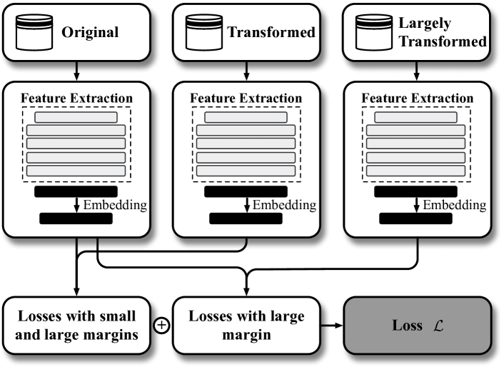
Figure 6. The architecture of the Siamese network used during the training phase.

Figure 6 shows the architecture of our Siamese network. Three kinds of data (original training data, transformed training data, and largely transformed training data) are given to the three models that share weights with each other. During the original classification training, the DNN classifier $M$ learns to extract meaningful and complex features in feature extraction layers before these are fed to the classification layers. To benefit from these rich representations of feature extraction layers, the Siamese network builds on $M$ to pass these features through a succession of dense layers. The outputs of the final dense layer are embeddings that will be used to minimize the loss function in equation 3. The function of the similarity measurement $f$ is the distance between the embeddings of two instances, formally, $f(a,b)=\big{\lVert}ebd(a)-ebd(b)\big{\rVert}_{2}^{2}$.

3.1.2. Distribution Discrimination

We designed the distribution analyzer to distinguish between the three kinds of data. In the training module, the embeddings of the original training data and validation data are generated from the trained Siamese network. For each validation data, its embedding is used to search for the closest one from the training data by the distance measure $f$. $\mathit{K}_{in}$ and $\mathit{K}_{out}$ are selected from the distances of embeddings between validation and training data. In deployment, given a test instance $x$, the minimum distance between its embedding and those of the training data will be a discriminator to determine its data category:

(4) $$\left\{\begin{array}[]{ll}\text{In-distribution data}&{min_{x_{t}\in\mathcal{X}^{t}}(f(x,x^{t}))<\mathit{K}_{in}}\\ \text{Out-of-distribution data}&{min_{x_{t}\in\mathcal{X}^{t}}(f(x,x^{t}))>\mathit{K}_{out}}\\ \text{Deviated data}&{others}\end{array}\right.$$

Note that unlike other enhanced classifier approaches (Wang et al., 2020; Xiao et al., 2021), InputReflector understands potential model prediction risks and can be made to discard runtime test instances that are unsuitable for model prediction (the Out-of-Distribution Alarm in Figure Figure 4).

3.2. Sample Reflector design

When the distribution analyzer recognizes an input instance as a deviation from the in-distribution data, the sample reflector will map this input to the closest sample in the training data. To build the sample reflector we adopt the idea of separation of concern (Pham and Triantaphyllou, 2008). That is, the subject model just needs to fit a limited number of samples in the training dataset, while the auxiliary model tackles the similarity measurement between training samples and their deviations. In other words, we let the subject model focus on fitting, and we task the auxiliary models with generalizability learning.

Next, we discuss the design of the sample reflector.

3.2.1. Quadruplet Network Training

Inspired by the work of Chen et al. (Chen et al., 2017) who built a deep quadruplet network for person re-identification, we construct a quadruplet network using the subject DNN classifier $M$ (similar to our Siamese network) to pull instances with the same label closer and push away instances with different labels. As illustrated in Figure 3, the goal of the Quadruplet network is to learn the feature embeddings so that instances of intra-class will be clustered together but those of inter-class will be further away. As a result, when an unexpected instance is presented, its embedding can be used to search for the closest samples from the training data, and these can be used as a proxy for identifying the input class.

1

2

Input: Target DNN classifier: $M$;

Input instances in $\mathit{D_{train}}$: $\mathcal{X}^{t}$, true labels in $\mathit{D_{train}}$: $\mathcal{Y}^{t}$;

Deviated test instance: $\mathcal{X}^{d}$

Output: Trained Quadruplet network;

Alternative predictions of the transformed test instance

3 # Training

4 $base\_model=M.get\_layer(``cnn").output$;

5 Add several dense layers after $base\_model$ to be embeddings $embed$;

6 $model=Model(base\_model.input,embed)$;

7 $model.compile(optimizer,Quadruplet\_loss)$;

8 $model.fit(\mathcal{X}^{t},\mathcal{Y}^{t})$;

9

10# Inference

11 $embed^{t}=model.predict(\mathcal{X}^{t})$;

12 for $\mathbf{x}$ in $\mathcal{X}^{d}$ do

13       $embed(x)=model.predict(x)$;

14       $idx^{T}=argmin(dist(embed(x),embed^{t}))$;

15       $predction_{new}=\mathcal{Y}^{T}[idx^{T}]$;

16      

17 end for

Algorithm 1 Quadruplet Network Training and Inference

Algorithm 1 lists the details of our Quadruplet network construction and how we use it in deployment. The Quadruplet network consist of the feature extraction layers of the target DNN classifier $M$ (line 2) and a succession of dense layers as shown in lines 2-4, which are trained by the quadruplet loss that is presented in Algorithm 2. This is an improvement over the triplet loss (Schroff et al., 2015) with an online component for mining the triplet online (Hermans et al., 2017).

During the construction of the Quadruplet network, the challenge is how to sample the quadruplet from the training data. Algorithm 2 discusses how to mine quadruplet samples during training. The sample mining process of the Siamese network in Section 3.1 also uses this technique.

1

2

Input: True labels in $\mathit{D_{train}}$: $\mathcal{Y}^{t}$;

Margins: $m_{1}$ and $m_{2}$;

Embeddings: $embed$

Output: loss

3 $pairwise\_dist=dist(embed)$;

4 obtain $mask$ where $mask[a,p]$ is True if $a$ and $p$ are distinct and have same label;

5 $dist_{ap}=mask*pairwise\_dist$;

6 $dist_{hard_{p}}=max(dist_{ap},axis=1)$;

7 obtain $mask$ where $mask[a,n]$ is True if $a$ and $n$ have distinct labels;

8 $max\_dist_{an}=max(pairwise\_dist,axis=1)$;

9 $dist_{an}=pairwise\_dist+max\_dist_{an}*(1.0-mask)$;

10 $dist_{hard_{n}}=min(dist_{an},axis=1)$;

11 $loss_{an}=mean(max(dist_{hard_{p}}-dist_{hard_{n}}+m_{1},0.0))$;

12 obtain $mask$ where $mask[a,p,n]$ is True if the triplet $(a,p,n)$ is valid;

13 $max\_dist_{an}=max(pairwise\_dist)$;

14 $dist_{an}=pairwise\_dist+max\_dist_{an}*(1.0-mask)$;

15 $dist_{hard_{nn}}=min(min(dist_{an},axis=2),axis=1)$;

16 $loss_{nn}=mean(max(dist_{hard_{p}}-dist_{hard_{nn}}+m_{2},0.0))$;

17 $loss=loss_{an}+loss_{nn}$;

18

Algorithm 2 Sampling in Quadruplet_loss

The loss of the Quadruplet network consists of two parts (Line 15 in Algorithm 1). The first part, $loss_{an}$, is the traditional triplet loss that is the main constraint. The second part, $loss_{nn}$, is auxiliary to the first loss and conforms to the structure of traditional triplet loss but has different triplets. We use two different margins ($m_{1}>m_{2}$) to balance the two constraints. We now discuss how to mine triplets for each loss.

First, a 2D matrix of distances between all the embeddings is calculated and stored in $pairwise\_dist$ (line 1). Given an anchor, we define the hardest positive example as having the same label as the anchor and whose distance from the anchor is the largest ($dist_{hard_{p}}$) among all the positive examples (lines 2-4). Similarly, the hardest negative example has a different label than the anchor and has the smallest distance from the anchor ($dist_{hard_{n}}$) among all the negative examples (lines 5-8). These hardest positive example and hardest negative example along with the anchor are formed as a triplet to minimizing $loss_{an}$ in line 9. After convergence, the maximum intra-class distance is required to be smaller than the minimum inter-class distance with respect to the same anchor.

To push away negative pairs from positive pairs, we introduce one more loss, $loss_{nn}$. Its aim is to make the maximum intra-class distance smaller than the minimum inter-class distance regardless of whether pairs contain the same anchor. This loss constrains the distance between positive pairs (i.e., samples with the same label) to be less than any other negative pairs (i.e., samples with different labels that are also different from the label of the corresponding positive samples). With the help of this constraint, the maximum intra-class distance must be less than the minimum inter-class distance regardless of whether pairs contain the same anchor. To mine such triplets, the valid triplet first needs to be filtered out on line 10 where $i,j,k$ are distinct and $(labels[i]\neq labels[j])\ \&\ (labels[i]\neq labels[k])\ \&\ (labels[j]\neq labels[k])$. Then, the hardest negative pairs are sampled whose distance is the minimum among all negative pairs in each batch during training (line 11-13). Finally $loss_{an}$ is minimized to further enlarge the inter-class variations in Line 14.

As discussed in (Chen et al., 2017), $(loss_{an}+loss_{nn})$ leads to a larger inter-class variation and a smaller intra-class variation as compared to the triplet loss. And this loss combination has a better generalization ability as will show in the evaluation (Section 4). The benefit of this arrangement is that the Quadruplet network can be used to help generalize the subject classifier $M$ to the unexpected deviations from in-distribution data.

3.2.2. Input Reflector for unexpected instances

Algorithm 1 lists the procedure for input reflection. Given an unexpected instance $x$ that belongs to the variated in-distribution data in deployment, the algorithm first obtains its feature embedding learned by the Quadruplet network (line 10). Next, the distance between $embed(x)$ and those embeddings of the training data generated in the training module (line 8) will be calculated so that the minimum distance can be found.

Finally, the unexpected test instance $x$ is then reflected to the specific training instance with the minimum distance whose label becomes the alternative prediction for $x$ (lines 11-12).

Now that we have detailed InputReflector’s design, we evaluate its performance on different datasets and DL models.

4. Evaluation

We now present experimental evidence for the effectiveness of InputReflector. Our evaluation goal is to answer the following research questions:

RQ1. Distribution Analyzer: How effective is the distribution analyzer in distinguishing three types of data? To evaluate the distribution analyzer, we compare its area under the receiver operating characteristic curve (AUROC) with related techniques, namely, Generalized ODIN (G-ODIN) (Hsu et al., 2020) and SelfChecker (Xiao et al., 2021). Specifically, we evaluate the performance of the distribution analyzer on detecting out-of-distribution and deviated data. Since the authors of G-ODIN did not release the code nor specific values for the hyperparameters, we implemented G-ODIN ourselves and used grid search to find the best combination of hyperparameters on the validation dataset, from which we obtained close results on the dataset in the G-ODIN paper. As there are two parts to SelfChecker, alarm and advice, to answer this RQ, we compare the distribution analyzer with SelfChecker’s alarm accuracy.

RQ2. Sample Reflector Accuracy: What is the accuracy of the reflection process on unseen deviated data? In cases where InputReflector recognizes the test instance as a deviation from in-distribution data, the reflection process will be used to provide an alternative prediction. To answer this question, we compare the accuracy of sample reflector (Section 3.2) in InputReflector against the accuracy of the subject model $M$ and advice accuracy of SelfChecker on the unseen deviated input.

RQ3. InputReflector Performance: What is the performance of InputReflector on the in-distribution and deviated input in deployment? Since the distribution analyzer is designed to learn $K_{in}$ and $K_{out}$ from transformed versions of training data (blur in this work), we compare the accuracy of InputReflector against the accuracy of original subject model ($M$), subject model with data augmentation ($M+Aug$), and SelfChecker on both pure in-distribution inputs and the deviating inputs.

RQ4. Overhead: What is the time/budget overhead of InputReflector in both training and deployment? To evaluate the efficiency of InputReflector, we calculated its overall time overhead with the ones of $M+Aug$ and SelfChecker. In the training phase, $M+Aug$ needs to conduct data generation and extra training. But, we regard the generation part as having zero cost and only consider the extra training time. Augmentation also does not have extra time cost in deployment. For SelfChecker and InputReflector, we measure their time overheads in training and deployment.

4.1. Experimental Setup

We evaluate the performance of InputReflector on three popular image datasets (MNIST (LeCun et al., 2010), FMNIST (Xiao et al., 2017), and CIFAR-10 (Krizhevsky et al., 2009)) using three DL models (ConvNet (Kim et al., 2019), VGG-16 (Simonyan and Zisserman, 2014), and ResNet-20 (He et al., 2016)). We conducted all experiments on a Linux server with Intel i9-10900X (10-core) CPU @ 3.70GHz, one RTX 2070 SUPER GPU, and 64GB RAM, running Ubuntu 18.04.

Our evaluation focuses on computer vision models. We hope to consider other types of models in future work. To evaluate InputReflector, we prepare three kinds of image datasets as follows:

In-distribution datasets. In-distribution data conform to the distribution of the training data. As in prior studies (Hsu et al., 2020; Liang et al., 2018; LEE et al., 2018), we regard the testing data of each dataset as the in-distribution data.

MNIST is a dataset for handwritten digit image recognition, containing 60,000 training images and 10,000 test images, with a total number of 70,000 images in 10 classes (the digits 0 through 9). Each MNIST image is a single-channel of size 28 * 28 * 1. Similarly, Fashion-MNIST is a dataset consisting of a training set of 60,000 images and a test set of 10,000 images. Each image is 28 * 28 grayscale images associated with a label from 10 classes. CIFAR-10 is a collection of images for general-purpose image classification, including 50,000 training data and 10,000 test data with 10 different classes (airplanes, cars, birds, cats, etc.). Each CIFAR-10 image is three-channel of size 32 * 32 * 3. The classification task of CIFAR-10 is generally harder than that of MNIST due to the size and complexity of the images in CIFAR-10.

Deviations from in-distribution datasets. We selected four kinds of transformations to construct the transformed data of in-distribution testing datasets: blur, bright, contrast, and zoom. These operations transform an image $x$ as follows (Gao et al., 2020):

• $zoom(x,d)$: zoom in $x$ with a zoom degree $d$ in range [1,5).

• $blur(x,d)$: blur $x$ using Gaussian kernel with a degree $d$ in range [0,5).

• $bright(x,d)$: uniformly add a value for each pixel of $x$ with a degree $d$ in range [0, 255) and then clip $x$ within [0, 255].

• $contrast(x,d)$: scale the RGB value of each pixel of $x$ by a degree $d$ in range (0, 1] and then clip $x$ within [0, 255].

We search for crash transformation degrees for each training and testing image on which the original classifier begins to mis-predict. The instances with such degrees then serve as the deviations of in-distribution data.

Out-of-distribution datasets. There are two kind of out-of-distribution data: the first one is the same as the existing work — another dataset which is completely different from the training data. The second one is the extremely transformed training and testing data using extreme degrees of the four transformations.

Specifically, we use FMNIST, MNIST, SVHN (Netzer et al., 2011) as the first totally different dataset for MNIST, FMNIST, CIFAR-10 respectively. The extremely transformed data cannot be recognized by both DL models and humans. We present the performance of the distribution analyzer on both dataset: another dataset and extremely transformed testing data.

DL models. We choose three DL models as our subject models: ConvNet, VGG-16, and ResNet-20. These are commonly-used models whose sizes range from small to large, with the number of layers ranging from 9 to 20.

Configurations. For fair comparison, the subject model $M$ does not use data augmentation. As discussed in Section 3.1 and 3.2, both the Siamese and Quadruplet networks are built on the subject model $M$, along with a succession of dense layers. We set the number of dense layers to be the same as the number of the classification layer in $M$. We use the Euclidean distance as the distance metric $f$ in (2).

Evaluation metrics. We adopt two measures to evaluate the distribution analyzer. AUROC plots the true positive rate (TPR) against the false positive rate (FPR) by varying a threshold, which can be regarded as an averaged score that can be interpreted as the model’s ability to discriminate between positive and negative inputs. TNR@TPR95 is the true negative rate at 95% true positive rate, which simulates an application requirement that the recall should be 95%. Having a high TNR under a high TPR is much more challenging than having a high AUROC score. We use classical model accuracy on testing data to evaluate the performance of both sample selector and InputReflector.

4.2. Results and Analyses

We now present results that answer our four research questions.

RQ1. Distribution Analyzer. Table 1 presents the AUROC and TNR@TPR95 of the distribution analyzer (Siamese) and Generalized ODIN (G-ODIN) to detect out-of-distribution data from in-distribution and deviated data. We exclude SelfChecker here because of its assumption on handling input that share similar semantics with the training dataset. As mentioned in Section 4.1, the out-of-distribution data here consists of totally differently data (same to the existing work) and extremely transformed data (blur, bright, contrast, and zoom), that’s why the results in Table 1 are different from previous work on detecting out-of-distribution from in-distribution data. Intuitively, distinguishing between the three data types is more difficult.

Based on Table 1, Siamese outperforms G-ODIN in most of the cases except for FMNIST on VGG-16. And we can see that both techniques have similar AUROC on FMNIST. The main reason is that Siamese cannot distinguish well between the deviated data and out-of-distribution data (MNIST here). When FMNIST data is contrasted, e.g., trouser, it will be similar to digit ”1”. For other settings, Siamese can not only detect totally different data as G-ODIN but also detect more extremely transformed data on which G-ODIN has bad performance. In average, Siamese achieves 80.52% AUROC against 71.02% of G-ODIN.

Table 1. Performance of two methods on detecting out-of-distribution data.

Out-of-distribution	AUROC			TNR@TPR95
	ConvNet	VGG-16	ResNet-20	ConvNet	VGG-16	ResNet-20
	G-ODIN/Siamese			G-ODIN/Siamese
blur
MNIST	69.50/69.29	60.88/85.15	78.00/78.38	13.67/50.11	02.00/56.23	45.37/48.25
FMNIST	73.99/69.85	71.51/57.58	74.86/75.50	37.16/50.05	38.26/28.40	27.17/44.98
CIFAR-10	77.09/79.97	45.28/85.28	73.70/76.51	52.69/55.70	04.44/36.95	40.96/39.94
bright
MNIST	58.77/73.70	60.23/81.83	89.00/88.11	21.66/49.96	38.30/46.43	57.01/67.57
FMNIST	78.62/84.70	74.14/73.45	73.79/76.82	40.18/59.94	49.54/33.03	33.02/41.62
CIFAR-10	77.04/95.39	44.77/86.90	77.00/82.71	55.20/79.80	04.34/37.69	46.65/60.06
contrast
MNIST	58.71/71.73	73.74/83.43	88.38/84.39	20.37/49.90	31.87/48.71	58.90/69.68
FMNIST	74.82/81.98	71.77/70.30	79.33/75.79	38.70/57.32	41.12/31.23	30.39/41.46
CIFAR-10	72.73/89.78	41.73/82.51	69.22/79.95	50.02/70.45	03.44/32.64	39.19/53.08
zoom
MNIST	67.43/85.15	66.85/77.19	75.24/82.75	03.97/54.38	03.82/43.96	32.92/56.41
FMNIST	81.28/83.77	70.67/70.10	81.56/83.05	44.66/57.68	33.30/31.66	37.57/51.03
CIFAR-10	88.25/94.35	47.60/90.11	88.92/91.11	64.49/74.78	05.87/40.93	53.71/56.82
Mean
MNIST	63.61/74.97	65.43/81.90	82.66/83.41	14.92/51.09	18.99/48.83	48.55/60.48
FMNIST	77.18/80.08	72.02/67.86	77.39/77.79	40.17/56.25	40.56/31.08	32.04/44.77
CIFAR-10	78.78/89.87	44.84/86.20	77.21/82.57	55.60/70.18	04.52/37.05	45.13/52.48

Table 2 compares the performance of G-ODIN, SelfChecker, and our distribution analyzer on detecting deviated data from in-distribution data on three DL models and three datasets with four transformations. Since SelfChecker is designed as a classifier, we omit its TNR@TPR95 here.

Except for CIFAR-10 on ConvNet, the distribution analyzer outperforms G-ODIN. The reason it fails is that ConvNet is too simple a DNN for CIFAR-10 on which Siamese cannot learn informative embeddings. But G-ODIN decomposed the softmax score to distinguish confident inputs from unconfident ones, which is hardly affected by the model architecture (Hsu et al., 2020).

In all other settings, Siamese achieves both high AUROC (averagely 91.84% against 75.01% of G-ODIN) and TNR@TPR95 (averagely 57.20% against 29.76% of G-ODIN) that is harder to reach. That means that Siamese can recognize more in-distribution data with the 95% recall of deviated data, which is important for the downstream reflection process. Given by the threshold search from validation dataset, Siamese can correctly detect on average 77.19% of deviated data. SelfChecker has bad performance since it is constrained by the assumption that the testing instance conform to the distribution of training dataset. But the deviated data here share similar semantics with the training data but are far away.

Table 2. Performance of three methods on detecting deviated data.

Deviated	AUROC			TNR@TPR95
	ConvNet	VGG-16	ResNet-20	ConvNet	VGG-16	ResNet-20
	G-ODIN/SelfChecker/Siamese			G-ODIN/Siamese
blur
MNIST	74.62/64.47/99.96	59.14/60.19/99.73	71.01/70.10/99.81	19.21/99.99	06.61/55.37	24.33/93.92
FMNIST	93.61/62.62/99.39	85.90/63.20/96.16	78.72/61.68/94.56	66.43/99.97	47.43/59.52	29.90/57.89
CIFAR-10	90.28/64.44/90.61	52.47/64.91/86.16	82.20/64.86/88.35	47.37/32.41	06.12/21.97	21.27/37.26
bright
MNIST	99.95/61.03/99.99	50.14/57.40/99.61	58.08/66.37/97.48	100.0/99.96	03.47/66.31	06.29/86.96
FMNIST	89.13/67.31/99.84	83.24/67.31/91.94	72.65/71.95/97.58	48.97/88.84	48.30/19.94	22.10/88.12
CIFAR-10	88.86/60.78/75.23	57.69/51.24/73.00	73.95/66.28/82.13	45.95/18.08	06.55/13.23	15.02/26.65
contrast
MNIST	99.93/60.12/99.99	66.79/69.29/99.62	55.13/64.17/97.12	100.0/100.0	04.58/61.18	05.39/84.30
FMNIST	90.82/54.90/99.90	76.06/45.69/95.51	71.76/63.97/97.77	55.98/90.46	26.93/29.09	24.01/88.41
CIFAR-10	93.37/58.14/75.87	63.95/56.07/87.35	85.32/64.15/89.39	64.07/16.24	11.33/29.13	24.64/35.79
zoom
MNIST	83.33/45.87/99.67	68.41/44.76/98.47	88.42/64.15/97.42	30.39/98.91	04.00/71.80	51.83/86.69
FMNIST	80.63/59.24/95.45	65.76/67.02/86.04	63.94/59.88/88.54	32.10/68.60	07.42/33.36	14.55/49.09
CIFAR-10	80.34/49.88/73.46	42.54/45.82/76.82	62.34/60.67/76.42	31.56/15.05	03.79/17.27	13.55/17.20
Mean
MNIST	89.46/57.87/99.91	61.12/57.91/99.36	68.16/66.20/97.96	62.40/99.72	04.67/63.67	21.96/87.97
FMNIST	88.55/61.02/98.65	77.74/60.81/92.41	71.77/64.37/94.62	50.87/86.97	32.52/35.48	22.64/70.88
CIFAR-10	88.21/58.31/78.79	54.16/54.51/80.83	75.95/63.99/84.07	47.24/20.45	06.95/20.40	18.62/29.23

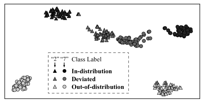
Figure 7. Visualization of the feature embedding learned by the Siamese network.

Figure 7 visualizes the separation between three types of data on MNIST with two labels (”2” and ”7”). This is generated from the learned embeddings from Siamese network and then mapped into hyperspace by t-SNE (Van der Maaten and Hinton, 2008). We can see that the three types of data are distant from each other and that the distance between in-distribution and deviated data is shorter than the distance between in-distribution and out-of-distribution data.

For RQ1, we conclude that the distribution analyzer has high performance in distinguishing three kinds of data. It can effectively detect out-of-distribution and deviated data with high accuracy.

RQ2. Sample Reflector Accuracy. Figure 8 compares the accuracies of the subject model $M$, SelfChecker, and the sample reflector on unseen deviating data. All four kinds of deviated data have not been seen by these models.

We find that the sample reflector achieves higher accuracy than $M$ and SelfChecker. The poor performance of SelfChecker is predictable since the deviating data does not strictly conform to the distribution of the training data.

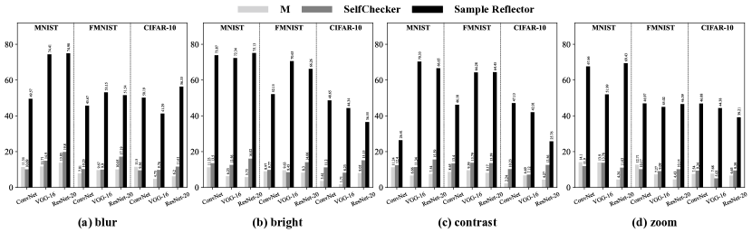
Figure 8. Accuracy of three methods on unseen deviated input.

For RQ2, we showed that the sample reflector prediction can improve the accuracy of the subject models on unseen deviating data.

RQ3. InputReflector Performance. To show the effectiveness of the proposed InputReflector, Table 3 presents the accuracies of the subject model $M$, $M$ with data augmentation ($M+Aug$), SelfChecker, and InputReflector on the in-distribution and deviating testing data. Both $M+Aug$ and InputReflector use the ”blur” version of the training data. $M+Aug$ enhances the original training data with its blurry version to retrain $M$. InputReflector uses blurry training data to train the auxiliary models, i.e., Siamese and Quadruplet network, instead of retraining M.

As we can see, SelfChecker cannot improve the $M$’s accuracy since it has poor performance in giving alternative prediction for deviating data. Both data augmentation (averagely 84.02%) and InputReflector (averagely 84.63%) improve the accuracy of $M$ (averagely 50.08%). The difference in their accuracies is not significant, which shows that InputReflector has similar generalization ability as data augmentation.

Table 3. Accuracy of four methods on the in-distribution and deviating testing data.

Accuracy	ConvNet	VGG-16	ResNet-20
	M/M+Aug/SelfChecker/InputReflector
blur
MNIST	55.16/99.38/57.19/99.36	55.65/99.55/60.45/99.02	56.65/99.44/55.39/99.40
FMNIST	50.04/93.67/54.30/92.48	51.94/94.41/55.14/91.44	51.40/91.60/52.17/91.57
CIFAR-10	45.84/78.43/47.29/76.08	46.85/88.59/44.39/88.42	43.91/79.50/50.78/79.20
bright
MNIST	55.10/93.14/56.09/92.11	52.91/96.49/59.81/95.22	52.59/91.64/60.37/94.43
FMNIST	50.62/75.13/49.82/81.18	51.92/75.32/56.12/77.40	50.53/80.17/60.25/84.65
CIFAR-10	41.89/64.88/47.94/65.23	45.33/70.99/48.45/77.43	44.84/65.73/46.86/65.14
contrast
MNIST	55.11/92.76/57.83/90.77	53.12/95.74/58.56/93.83	53.49/92.67/60.06/94.62
FMNIST	50.46/75.73/59.26/80.09	51.90/76.30/58.30/77.10	50.46/80.69/57.95/86.66
CIFAR-10	41.21/74.87/42.64/75.92	47.82/79.96/49.18/83.14	42.95/72.88/45.83/72.76
zoom
MNIST	56.54/90.52/57.23/85.92	56.74/84.90/56.38/84.87	51.89/83.32/59.43/90.37
FMNIST	52.49/79.56/51.65/78.49	50.74/84.90/50.28/81.66	48.59/80.59/49.54/81.54
CIFAR-10	43.86/76.41/49.25/77.06	48.32/86.39/50.03/84.09	44.13/78.38/53.56/78.26
Mean
MNIST	55.47/93.95/57.09/92.04	54.60/94.17/58.80/93.23	53.65/91.77/58.81/94.70
FMNIST	50.90/81.02/53.76/83.06	51.62/82.73/54.96/81.90	50.24/83.26/54.98/86.10
CIFAR-10	43.20/73.65/46.78/73.57	47.08/81.48/48.01/83.27	43.95/74.12/49.26/73.84

However, not all data used in data augmentation can enhance $M$. For example, the accuracy of $M$ will degrade when using adversarial example for data augmentation.

To show the sensitivity of $M+Aug$ and InputReflector on adversarial/poisonous data, we include both adversarial and blurry training data for both methods. Table 4 shows the mean accuracies of $M+Aug$ and InputReflector on the in-distribution data and the one plus deviating data with the four transformations.

The lowest accuracies of $M+Aug$ on in-distribution data indicate that data augmentation with adversarial examples will harm model performance even on the normal testing data. But, InputReflector is more tolerant and it does not effect the accuracy of in-distribution data. But, the generalization ability of both methods are reduced, as indicated by the lower accuracies on in-distribution and deviating data than when only using blurry training data as augmentation. The tolerance of InputReflector benefits from the sample mining in both Siamese and Quadruplet networks where many adversarial examples are filtered out.

Table 4. Accuracy using adversarial examples as data augmentation.

Accuracy	In-distribution			In-distribution+Deviated
	ConvNet	VGG-16	ResNet-20	ConvNet	VGG-16	ResNet-20
	M/M+Aug/InputReflector			M/M+Aug/InputReflector
MNIST	98.97/97.46/99.57	99.58/97.54/99.65	99.44/98.31/99.48	55.47/88.52/89.20	54.60/90.67/94.38	53.65/93.00/94.81
FMNIST	92.27/92.08/92.27	94.20/92.20/94.57	92.75/91.34/93.58	50.90/79.50/82.03	51.62/80.38/85.99	50.24/80.89/83.05
CIFAR-10	80.17/76.80/80.71	88.95/87.59/89.31	81.62/75.38/82.96	43.20/68.73/66.31	47.08/76.35/79.01	43.95/64.39/67.07

To answer RQ3, InputReflector has similar generalization ability as data augmentation and can detect out-of-distribution data but data augmentation doesn’t have such mechanism. And InputReflector is more tolerant than data augmentation when considering adversarial examples.

RQ4. Overhead. We measured the time consumption of $M+Aug$, SelfChecker, and InputReflector during training and deployment. Table 5 shows that $M+Aug$ and InputReflector cost similar training time where SelfChecker costs the most since it needs to estimate the distribution of each layer. For each test instance in deployment, InputReflector needs more time overhead than $M+Aug$ because of the distance calculation and closet training data search. But its time consumption is much lower than SelfChecker.

Table 5. Time overhead.

Time	M+Aug	Selfchecker	InputReflector
Training	41.97m	¿1h	39.5m
Deployment	0.98s	34.33s	2.86s

5. Related Work

InputReflector contains two elements: a distribution analyzer to detect out-of-distribution and deviated data, and a sample reflector. In this section, we will discuss previous work related to both of these elements.

Detection of out-of-distribution data. Several methods (Liang et al., 2018; LEE et al., 2018; Hsu et al., 2020) have been proposed to detect out-of-distribution data that is completely different from the training data. ODIN (Liang et al., 2018) and Generalized ODIN (Hsu et al., 2020) are based on trained neural network classifiers that must be powerful enough for the specific dataset. In (Liang et al., 2018; Hsu et al., 2020), the authors modified the last softmax layer to statistically distinguish in-distribution and out-of-distribution data. The max class probability of the softmax layer are mapped into a hyperspace by temperature scaling and input pre-processing to create a more effective score that can distinguish the distributions of out-of-distribution and in-distribution data. Hsu et al. (Hsu et al., 2020) introduced a decomposed confidence function to avoid using out-of-distribution data to train the classifier, as was done by Liang et al. (Liang et al., 2018). The decomposed confidence function splits the original softmax function into two parts to avoid issues with overconfidence.

The internal representation of DNN models given an input has also been used to detect out-of-distribution data. Mahalanobis (LEE et al., 2018) takes hidden layers of the DNN model as representation spaces. This work used the distance calculation and input pre-processing to compute the Mahalanobis distance to measure the extent to which an input belongs to the in-distribution in these spaces. But there is a hyperparameter in input pre-processing that need to be tuned for each out-of-distribution dataset.

None of these techniques detect deviated data that is between in-distribution and out-of-distribution data, which is the key feature of our InputReflector. Hsu et al. (Hsu et al., 2020) showed that Generalized ODIN is empirically superior to previous approaches (Hendrycks and Gimpel, 2016; Liang et al., 2018; LEE et al., 2018); we therefore use Generalized ODIN as our baseline to evaluate the performance of the distribution analyzer in InputReflector.

Data augmentation. To improve the DNN model generalization, data augmentation techniques have been proposed (Gao et al., 2020; Samangouei et al., 2018; Zhong et al., 2020; Dreossi et al., 2018). In a recent work in this space, Guo et al. (Gao et al., 2020) augment training data using mutation-based fuzzing. The authors specifically focus on improving the robust generalization of DNNs. A model with robust generalization should not degrade in performance for train/test data with small perturbations such as applying spatial transformations to images). By drawing a parallel between training DNNs and program synthesis, mutation-based fuzzing is used for data augmentation and the computational cost has been further reduced by selecting only a part of data for augmentation. But, our experimental results indicate that DNN model accuracy on normal testing data will quickly degrade if the training data is augmented with data containing large perturbations. The aim of InputReflector is therefore to improve model generalization without sacrificing its accuracy. Another problem with data augmentation is that even an augmented training dataset is ultimately finite, limiting model generalization.

Runtime trustworthiness checking. In the software engineering community, several studies consider checking a DNN’s trustworthiness in deployment. DISSECTOR proposed by Wang et al. (Wang et al., 2020) detects inputs that deviate from normal inputs. It trains several sub-models on top of the pre-trained model to validate samples fed into the model. Xiao et al. (Xiao et al., 2021) propose SelfChecker to monitor DNN outputs using internal layer features. It trigger an alarm if the internal layer features of the model are inconsistent with the final prediction and also provides an alternative prediction. The assumption in these two papers is that the training and validation datasets come from a distribution similar to that of the inputs that the DNN model will face in deployment. For example, SelfChecker cannot detect out-of-distribution data and provides an alarm constrained by this assumption. SelfChecker’s ability of analyze unseen deviating data is also weak, not to mention provide predictions for such input.

6. Conclusion

Deployed DNNs must contend with inputs that may contain noise or distribution shifts. Even the best-performing DNN model in training may make wrong predictions on such inputs. We presented an input reflection approach to deal with this issue. Input reflection first determines that the input is problematic and then reflects it towards a nearby sample in the training dataset. Unlike previous work, this reflection strategy focuses on characteristics of the input and allows for fine-grained control and better understanding of precisely when and how the technique works. We implemented input reflection as part of the InputReflector tool and evaluated it empirically across several datasets and model variants. On the three popular image datasets with four transformations InputReflector is able to distinguish unseen problematic inputs with an average accuracy of 77.19%. Furthermore, by combining InputReflector with the original DNN, we can increase the average model prediction accuracy by 34.55% on the in-distribution and deviated testing dataset. Moreover, InputReflector can detect out-of-distribution data that the original DNN cannot handle. We hope that our work inspires further research into characterizing the deployment-time inputs in the context of the DNN training dataset.

References

- (1)
- Bromley et al. (1993) Jane Bromley, James W Bentz, Léon Bottou, Isabelle Guyon, Yann LeCun, Cliff Moore, Eduard Säckinger, and Roopak Shah. 1993. Signature verification using a “siamese” time delay neural network. International Journal of Pattern Recognition and Artificial Intelligence 7, 04 (1993), 669–688.
- Chen et al. (2017) Weihua Chen, Xiaotang Chen, Jianguo Zhang, and Kaiqi Huang. 2017. Beyond triplet loss: a deep quadruplet network for person re-identification. In Proceedings of the IEEE conference on computer vision and pattern recognition. 403–412.
- Chicco (2021) Davide Chicco. 2021. Siamese neural networks: An overview. Artificial Neural Networks (2021), 73–94.
- Ciresan et al. (2012) Dan Ciresan, Alessandro Giusti, Luca M Gambardella, and Jürgen Schmidhuber. 2012. Deep Neural Networks Segment Neuronal Membranes in Electron Microscopy Images. In Advances in neural information processing systems. 2843–2851.
- Dreossi et al. (2018) Tommaso Dreossi, Shromona Ghosh, Xiangyu Yue, Kurt Keutzer, Alberto Sangiovanni-Vincentelli, and Sanjit A Seshia. 2018. Counterexample-guided data augmentation. arXiv preprint arXiv:1805.06962 (2018).
- Ganin et al. (2016) Yaroslav Ganin, Evgeniya Ustinova, Hana Ajakan, Pascal Germain, Hugo Larochelle, François Laviolette, Mario Marchand, and Victor Lempitsky. 2016. Domain-adversarial training of neural networks. The journal of machine learning research 17, 1 (2016), 2096–2030.
- Gao et al. (2020) Xiang Gao, Ripon K Saha, Mukul R Prasad, and Abhik Roychoudhury. 2020. Fuzz testing based data augmentation to improve robustness of deep neural networks. In 2020 IEEE/ACM 42nd International Conference on Software Engineering (ICSE). IEEE, 1147–1158.
- Gao et al. (2021) Zhan Gao, Alejandro Ribeiro, and Fernando Gama. 2021. Wide and deep graph neural networks with distributed online learning. In ICASSP 2021-2021 IEEE International Conference on Acoustics, Speech and Signal Processing (ICASSP). IEEE, 5270–5274.
- He et al. (2016) Kaiming He, Xiangyu Zhang, Shaoqing Ren, and Jian Sun. 2016. Deep residual learning for image recognition. In Proceedings of the IEEE conference on computer vision and pattern recognition. 770–778.
- Hendrycks and Gimpel (2016) Dan Hendrycks and Kevin Gimpel. 2016. A baseline for detecting misclassified and out-of-distribution examples in neural networks. arXiv preprint arXiv:1610.02136 (2016).
- Hermans et al. (2017) Alexander Hermans, Lucas Beyer, and Bastian Leibe. 2017. In defense of the triplet loss for person re-identification. arXiv preprint arXiv:1703.07737 (2017).
- Hsu et al. (2020) Yen-Chang Hsu, Yilin Shen, Hongxia Jin, and Zsolt Kira. 2020. Generalized odin: Detecting out-of-distribution image without learning from out-of-distribution data. In Proceedings of the IEEE/CVF Conference on Computer Vision and Pattern Recognition. 10951–10960.
- Ilyas et al. (2019) Andrew Ilyas, Shibani Santurkar, Logan Engstrom, Brandon Tran, and Aleksander Madry. 2019. Adversarial Examples Are Not Bugs, They Are Features. Advances in neural information processing systems 32 (2019).
- Kim et al. (2019) Jinhan Kim, Robert Feldt, and Shin Yoo. 2019. Guiding Deep Learning System Testing Using Surprise Adequacy. In 2019 IEEE/ACM 41st International Conference on Software Engineering (ICSE). IEEE, 1039–1049.
- Kim et al. (2020) Sungyeon Kim, Dongwon Kim, Minsu Cho, and Suha Kwak. 2020. Proxy anchor loss for deep metric learning. In Proceedings of the IEEE/CVF Conference on Computer Vision and Pattern Recognition. 3238–3247.
- Koch et al. (2015) Gregory Koch, Richard Zemel, Ruslan Salakhutdinov, et al. 2015. Siamese neural networks for one-shot image recognition. In ICML deep learning workshop, Vol. 2. Lille.
- Krizhevsky et al. (2009) Alex Krizhevsky, Geoffrey Hinton, et al. 2009. Learning Multiple Layers of Features from Tiny Images. (2009). https://www.cs.toronto.edu/~kriz/cifar.html
- LeCun et al. (2010) Yann LeCun, Corinna Cortes, and CJ Burges. 2010. MNIST Handwritten Digit Database. (2010). http://yann.lecun.com/exdb/mnist/
- LEE et al. (2018) KIMIN LEE, Kibok Lee, Honglak Lee, and Jinwoo Shin. 2018. A Simple Unified Framework for Detecting Out-of-Distribution Samples and Adversarial Attacks. In 32nd Conference on Neural Information Processing Systems (NIPS). Neural Information Processing Systems Foundation.
- Li et al. (2019) Bo Li, Wei Wu, Qiang Wang, Fangyi Zhang, Junliang Xing, and Junjie Yan. 2019. Siamrpn++: Evolution of siamese visual tracking with very deep networks. In Proceedings of the IEEE/CVF Conference on Computer Vision and Pattern Recognition. 4282–4291.
- Liang et al. (2018) Shiyu Liang, Yixuan Li, and R Srikant. 2018. Enhancing The Reliability of Out-of-distribution Image Detection in Neural Networks. In International Conference on Learning Representations.
- Long et al. (2015) Jonathan Long, Evan Shelhamer, and Trevor Darrell. 2015. Fully convolutional networks for semantic segmentation. In Proceedings of the IEEE conference on computer vision and pattern recognition. 3431–3440.
- Miyato et al. (2016) Takeru Miyato, Andrew M Dai, and Ian Goodfellow. 2016. Adversarial training methods for semi-supervised text classification. arXiv preprint arXiv:1605.07725 (2016).
- Netzer et al. (2011) Yuval Netzer, Tao Wang, Adam Coates, Alessandro Bissacco, Bo Wu, and Andrew Y Ng. 2011. Reading digits in natural images with unsupervised feature learning. (2011).
- Pham and Triantaphyllou (2008) Huy Nguyen Anh Pham and Evangelos Triantaphyllou. 2008. Prediction of diabetes by employing a new data mining approach which balances fitting and generalization. In Computer and Information Science. Springer, 11–26.
- Qian et al. (2019) Qi Qian, Lei Shang, Baigui Sun, Juhua Hu, Hao Li, and Rong Jin. 2019. Softtriple loss: Deep metric learning without triplet sampling. In Proceedings of the IEEE/CVF International Conference on Computer Vision. 6450–6458.
- Redmon et al. (2016) Joseph Redmon, Santosh Divvala, Ross Girshick, and Ali Farhadi. 2016. You only look once: Unified, real-time object detection. In Proceedings of the IEEE conference on computer vision and pattern recognition. 779–788.
- Samangouei et al. (2018) Pouya Samangouei, Maya Kabkab, and Rama Chellappa. 2018. Defense-gan: Protecting classifiers against adversarial attacks using generative models. arXiv preprint arXiv:1805.06605 (2018).
- Schroff et al. (2015) Florian Schroff, Dmitry Kalenichenko, and James Philbin. 2015. Facenet: A unified embedding for face recognition and clustering. In Proceedings of the IEEE conference on computer vision and pattern recognition. 815–823.
- Shafahi et al. (2019) Ali Shafahi, Mahyar Najibi, Amin Ghiasi, Zheng Xu, John Dickerson, Christoph Studer, Larry S Davis, Gavin Taylor, and Tom Goldstein. 2019. Adversarial training for free! arXiv preprint arXiv:1904.12843 (2019).
- Shrivastava et al. (2017) Ashish Shrivastava, Tomas Pfister, Oncel Tuzel, Joshua Susskind, Wenda Wang, and Russell Webb. 2017. Learning from simulated and unsupervised images through adversarial training. In Proceedings of the IEEE conference on computer vision and pattern recognition. 2107–2116.
- Simonyan and Zisserman (2014) Karen Simonyan and Andrew Zisserman. 2014. Very Deep Convolutional Networks for Large-scale Image Recognition. arXiv:1409.1556 (2014).
- Taigman et al. (2014) Yaniv Taigman, Ming Yang, Marc’Aurelio Ranzato, and Lior Wolf. 2014. Deepface: Closing the gap to human-level performance in face verification. In Proceedings of the IEEE conference on computer vision and pattern recognition. 1701–1708.
- Van der Maaten and Hinton (2008) Laurens Van der Maaten and Geoffrey Hinton. 2008. Visualizing data using t-SNE. Journal of machine learning research 9, 11 (2008).
- Wang et al. (2020) Huiyan Wang, Jingwei Xu, Chang Xu, Xiaoxing Ma, and Jian Lu. 2020. Dissector: Input validation for deep learning applications by crossing-layer dissection. In 2020 IEEE/ACM 42nd International Conference on Software Engineering (ICSE). IEEE, 727–738.
- Wang et al. (2019a) Jingyi Wang, Guoliang Dong, Jun Sun, Xinyu Wang, and Peixin Zhang. 2019a. Adversarial sample detection for deep neural network through model mutation testing. In 2019 IEEE/ACM 41st International Conference on Software Engineering (ICSE). IEEE, 1245–1256.
- Wang et al. (2019b) Run Wang, Felix Juefei-Xu, Lei Ma, Xiaofei Xie, Yihao Huang, Jian Wang, and Yang Liu. 2019b. Fakespotter: A simple yet robust baseline for spotting ai-synthesized fake faces. arXiv preprint arXiv:1909.06122 (2019).
- Xiao et al. (2017) Han Xiao, Kashif Rasul, and Roland Vollgraf. 2017. Fashion-mnist: a novel image dataset for benchmarking machine learning algorithms. arXiv preprint arXiv:1708.07747 (2017).
- Xiao et al. (2021) Yan Xiao, Ivan Beschastnikh, David S Rosenblum, Changsheng Sun, Sebastian Elbaum, Yun Lin, and Jin Song Dong. 2021. Self-Checking Deep Neural Networks in Deployment. In 2021 IEEE/ACM 43rd International Conference on Software Engineering (ICSE). IEEE, 372–384.
- Zhang et al. (2020) Xiyue Zhang, Xiaofei Xie, Lei Ma, Xiaoning Du, Qiang Hu, Yang Liu, Jianjun Zhao, and Meng Sun. 2020. Towards characterizing adversarial defects of deep learning software from the lens of uncertainty. In 2020 IEEE/ACM 42nd International Conference on Software Engineering (ICSE). IEEE, 739–751.
- Zhang and Peng (2019) Zhipeng Zhang and Houwen Peng. 2019. Deeper and wider siamese networks for real-time visual tracking. In Proceedings of the IEEE/CVF Conference on Computer Vision and Pattern Recognition. 4591–4600.
- Zhong et al. (2020) Zhun Zhong, Liang Zheng, Guoliang Kang, Shaozi Li, and Yi Yang. 2020. Random erasing data augmentation. In Proceedings of the AAAI Conference on Artificial Intelligence, Vol. 34. 13001–13008.