Knothe-Rosenblatt transport for Unsupervised Domain Adaptation

Abstract

Unsupervised domain adaptation (UDA) aims at exploiting related but different data sources to tackle a common task in a target domain. UDA remains a central yet challenging problem in machine learning. In this paper, we present an approach tailored to moderate-dimensional tabular problems which are hugely important in industrial applications and less well-served by the plethora of methods designed for image and language data. Knothe-Rosenblatt Domain Adaptation (KRDA) is based on the Knothe-Rosenblatt transport: we exploit autoregressive density estimation algorithms to accurately model the different sources by an autoregressive model using a mixture of Gaussians. KRDA then takes advantage of the triangularity of the autoregressive models to build an explicit mapping of the source samples into the target domain. We show that the transfer map built by KRDA preserves each component quantiles of the observations, hence aligning the representations of the different data sets in the same target domain. Finally, we show that KRDA has state-of-the-art performance on both synthetic and real world UDA problems.

1 Introduction

In classical machine learning, we assume that both the training and test data follow the same distribution and we can thus expect to generalize from the training set to the test set. In practice, this assumption does not always hold. For example, data is often collected in asynchronous manner, at different times and locations, and may be labeled by different people, which can affect the efficiency and quality of the standard supervised learning models (Quionero-Candela et al., 2009; Pan and Yang, 2010). Collecting data from multiple sources may also lead to distribution shift between the collectors. For example, wireless network data would present different properties and patterns depending on time (such as day, night, week-end), or location/ infrastructure (downtown, countryside, or touristic area). Even when the task is common, an efficient approach should take into account the shift. Coping with this problem lead to the development of transfer learning methods that adapt the knowledge from a source domain to a new target domain.

Transfer learning, or domain adaptation, is central in vision (image classification, image segmentation, or activity recognition) (Li et al., 2020b) and natural language processing (translation, language generation) (Malte and Ratadiya, 2019; Ruder et al., 2019) problems. Both of these domains generate very high-dimensional data, and transfer learning usually focuses on fine tuning pre-trained models to specific tasks. In contrast, the principal problem in many industrial applications is not dimensionality, rather class imbalance, probability shift in data collection, and small data (Zhang et al., 2019). For example, wireless network data (5G and beyond), IoT or smart cities are often low dimensional (less than $100$), and highly dependent on the data collection context (Fu et al., 2018; Arjoune and Faruque, 2020; Benzaid and Taleb, 2020). These issues are rarely dealt within the transfer learning literature.

Transfer learning on high-dimensional data usually proceeds by mapping the data into a smaller dimensional space and carrying out the transfer in this latent space. In the lower dimensional domain we are targeting, we can use recently developed powerful density estimation techniques and principled transport-based approaches that rely on these precise estimates.

Our contribution is Knothe-Rosenblatt Domain Adaptation, or KRDA. We tackle Domain Adaptation (DA) which arises when the probability distribution of the source and the target data are different but related. We focus on the more challenging task where we do not have labeled target data. This approach, called Unsupervised Domain Adaptation, is the most difficult case of distribution shift. We estimate the density of both the source and the target data in order to transfer the former to the later. We use RNADE (Uria et al., 2013), an autoregressive technique that decomposes the $d$-dimensional density into $d$ one-dimensional conditional densities, represented by input dependent mixtures of Gaussian (also known as mixture density nets  (Bishop, 1994)). Using these explicit representations, KRDA transfers each sample by preserving the conditional quantiles with Knothe-Rosenblatt transport. Once embedded in the target domain, the source and its labels are learned by a supervised learning algorithm. Although theoretically simple, using autoregressive models in order to perform a transport has not yet been considered in the transfer learning literature.

As it will be illustrated, KRDA is particularly well suited for small data (less than $10000$ samples) in small dimension (less than $100$), where other state-of-the-art methods tend to under-perform, as shown in Section 6. We can also consider KRDA as an embedding algorithm with a great advantage: all the extra-computational cost of KRDA is spent in the computation of the transfer map. Once the source is transferred, training and testing will have no overhead beyond the cost of the supervised learning algorithm used.

The paper is structured as follows. We first introduce KRDA, an algorithm based on density estimation. We review some topics in density estimation in Section 4. We then introduce KRDA, the core of our paper, in Section 5, and expose its properties and limitations. Finally we compare our approach against state-of-the-art transfer learning algorithms on several benchmark. A detailed experimental setting and the results are given in Section 6.

2 Related work

Transfer learning (TL) aims at building algorithms that generalize across different domains with different probability distributions, see for example (Pan and Yang, 2010; Kouw and Loog, 2019; Zhuang et al., 2019) for global surveys of the field. Domain adaptation is the specific case when the task is the same across the different domains. DA approaches may be roughly divided in two categories depending on whether we have access to labels in the target space, or not. The first case is known as semi-supervised DA. The usual approach is to find a global transformation that aligns the different domains by preserving the information coming from a few labels (Saenko et al., 2010). Many papers embed both domains in the same latent space using different tools such as similarity (Donahue et al., 2013), non-linear kernel mapping (Pan et al., 2010; Gong et al., 2016), or entropy (Saito et al., 2019).

In unsupervised domain adaptation, we assume that we have no labels from the target domain. One avenue is to reweight the samples in order to correct the shift between the source and target distributions (Huang et al., 2007; Gretton et al., 2007). This method has the advantage of not requiring distribution estimation or specific embedding. As in semi-supervised DA, other unsupervised approaches rely on a common latent space. Both the source and target data are projected into this space, and a classifier is then learned using the labeled source data in the latent space. Another shallow approach, subspace mapping, aims at learning a linear map that aligns source and target (Gong et al., 2012; Fernando et al., 2013; Sharma et al., 2012).

More recently, deep neural nets became a popular choice in UDA due to the flexibility of these models to learn rich non-linear mappings. Deep Adaptation Network (Long et al., 2015) adds multiple kernel variants of MMD at the top layers to push the target distribution close to the source. Domain-Adversarial Neural Network (Ganin et al., 2016) introduces adversarial training to reduce the distance between the source and target feature distributions. Joint Adaptation Networks (Long et al., 2017) and Conditional Adversarial Domain Adaptation (Long et al., 2018) aim at aligning the joint or conditional distributions. Instead of learning transferable representations, Saito et al. (2018) align the source and target distributions by maximizing the discrepancy between the outputs of two classifiers. Using clustering is another approach (Shu et al., 2018; Liang et al., 2020; Li et al., 2020a).

In this paper we use recently developed powerful density estimators to relate the source and target domains. Density estimation is an important problem in statistics in general and machine learning in particular (Bishop, 1994; Wasserman, 2004). Among the plethora of methods (Salakhutdinov and Hinton, 2009; 458, ; Rezende and Mohamed, 2015; Ho et al., 2019), we use autoregressive models for their triangularity that is crucial for our approach (Larochelle and Murray, 2011; Uria et al., 2013). These algorithms model the joint distribution as product of one-dimensional conditional densities using the probability chain rule. They take advantage of recent developments in recurrent neural networks (Oord et al., 2016). A drawback of this approach is the fixed arbitrary ordering of the components, although it seems not to be crucial in many applications (Kégl et al., 2021), including ours, arguably explained by the flexibility of the mixtures that can model the potentially complex conditional densities.

Optimal transport sees the domain adaptation problem as graph matching (Courty et al., 2017) and embed the source into the target by minimizing a transportation cost. Knothe-Rosenblatt transport has been independently introduced in (Rosenblatt, 1952; Knothe, 1957), the former for multivariate statistics analysis and the latter to study isoperimetric inequality problems. This approach has been applied for histogram equalization for RGB pictures (Pitié et al., 2007). More recently, (Muzellec and Cuturi, 2019) use a generalization of Knothe-Rosenblatt transport as a surrogate to optimal transport in high dimensional spaces: the paper fits a multi-dimensional GMM that is transferred at once.

3 Background and notations

We consider the setting of classical transfer learning. The fundamental objective is to use some knowledge acquired during the learning of a specific predictive task in order to perform a similar but different task. More precisely, the domain $\mathcal{D}$ of a learning task is a couple composed of a feature space $\mathcal{X}$ and a marginal probability distribution $p(X)$. A task is a couple $(\mathcal{Y},f)$ composed of a label space $\mathcal{Y}$ and a prediction function $f:\mathcal{X}\rightarrow\mathcal{Y}$. In transfer learning, we consider two domains and learning tasks named source $(\mathcal{D}_{\mathcal{S}},\mathcal{Y}_{\mathcal{S}})$ and target $(\mathcal{D}_{\mathcal{T}},\mathcal{Y}_{\mathcal{T}})$. In the transfer learning setting $(\mathcal{X}_{\mathcal{S}},p_{\mathcal{S}})\neq(\mathcal{X}_{\mathcal{T}},p_{\mathcal{T}})$ and the goal is to transfer some knowledge from the source to the target. There are several sub-cases such as covariate shift, on which KRDA relies, in which $p_{\mathcal{S}}(x)\neq p_{\mathcal{T}}(x)$ but the conditional probabilities are invariant: $p_{\mathcal{S}}(y|x)=p_{\mathcal{T}}(y|x)$ for every $y\in\mathcal{Y}$.

In the unsupervised setting we have no access to the labels of the target data. We thus aim at building a transfer map $T:\mathcal{X}_{\mathcal{S}}\rightarrow\mathcal{X}_{\mathcal{T}}$ which associates a vector in the target feature space to every source sample before applying a classifier.

Let $D_{\mathcal{S}}=(X_{\mathcal{S}},Y_{\mathcal{S}})$ and $D_{\mathcal{T}}=(X_{\mathcal{T}},Y_{\mathcal{T}})$ be the source and target data sets, respectively. Let $p_{\mathcal{S}}$ and $p_{\mathcal{T}}$ be the probability density functions (PDF) of the source data $X_{\mathcal{S}}$ and target data $X_{\mathcal{T}}$, and let $\hat{p}_{\mathcal{S}}$ and $\hat{p}_{\mathcal{T}}$ be the estimated densities, respectively. We will denote by $F_{p}$ the cumulative density function (CDF) associated with the density $p$. For a vector function $g:\mathbb{R}^{m}\rightarrow\mathbb{R}^{n}$ and $x\in\mathbb{R}^{m}$, let $g^{i}(x)\in\mathbb{R}$ be the $i$-th coefficient of $g(x)$.

4 Autoregressive density estimation

In this work, we will focus on autoregressive models. The probability density function is expressed using the probability chain rule: the PDF of a vector $x=(x^{1},\dots,x^{d})\in\mathbb{R}^{d}$ is the product of one-dimensional conditional densities

$$p(x)=\prod_{i=1}^{d}p^{i}(x^{i}|x^{<i}).$$ (1)

Each conditional factor density will be approximated by a Gaussian mixture distribution. Note that this straightforwardly generalizes to any type of mixture distribution, although we will focus on Gaussian mixtures in this paper for didactic purposes.

RNADE (Uria et al., 2013) is a robust and flexible deep learning method that, following Eq. (1), fits one-dimensional conditional Gaussian mixtures (originally proposed by (Bishop, 1994) under the name of mixture density net (MDN)) for every coefficient of a vector $x=(x^{1},\dots,x^{d})\in\mathbb{R}^{d}$. More precisely we associate to each conditional probability $p^{i}(x^{i}|x^{<i})$ a distribution composed of a mixture of $N$ Gaussians $\sum_{k=1}^{N}w_{k}^{i}\mathcal{N}(\mu_{k}^{i},\sigma_{k}^{i})$. The RNADE algorithm with hidden size $H$ is based on NADE (Larochelle and Murray, 2011) and can be summarized as follows. We first compute from the input $x=(x^{1},\dots,x^{d})$ the sequence $a^{i}\in\mathbb{R}^{H}$, $i=1,\ldots,d$, in an iterative manner:

$$a^{1}=c; a^{i+1}=a^{i}+x^{i}W_{\cdot,i},$$ (2)

where $c\in\mathbb{R}^{H}$ and $W\in\mathbb{R}^{H\times d}$ are learned parameters, and $W_{\cdot,i}$ denotes the $i$th column of the parameter matrix $W$. We then apply a non-linearity after re-scaling

$$h^{i}=\sigma(C^{i}a^{i})$$ (3)

to get the parameters of the conditional Gaussian mixture as output of linear layers:

$$w^{i} =\operatorname{Softmax}(\operatorname{Lin}_{1}(h^{i})),$$ (4)

$$\mu^{i} =\operatorname{Lin}_{2}(h^{i}),$$ (5)

$$\sigma^{i} =\exp(0.5\times\operatorname{Lin}_{3}(h^{i}))\,,$$ (6)

where $\operatorname{Lin}_{1}$, $\operatorname{Lin}_{2}$, $\operatorname{Lin}_{3}$ are three linear layers $\mathbb{R}^{H}\rightarrow\mathbb{R}^{N}$ with bias. In this work, we use $\sigma=\operatorname{RELU}$ as the non-linearity applied in (3). The exact likelihood is thus directly accessible, and the model is trained end-to-end by maximizing the log-likelihood using gradient ascent. Note that this density estimator also makes data generation from the estimated distribution easy (go through the chain Eq. (1) and sample from Gaussian mixtures).

In domain adaptation, we make the assumption of having related distributions for the source and the target data. In order for the density estimation model to use this assumption, we share the parameters $c$ and $W$ in Eq. (2) for all data sets. The last linear layer of Eqs. (4-6) are specific to the source and target and will capture the dissimilarities between the domains. The density estimation network is then trained simultaneously on both the source and the target data.

5 Knothe-Rosenblatt transport

Having two densities $p_{\mu}$ and $p_{\nu}$, there are several ways to built a transport place $T$ such that $T_{\sharp}\mu=\nu$. For example, the change of variable formula $p_{\mu}=p_{\nu}(T(x))\det(Jac_{x}T)$ defines a PDE for which $T$ is solution (assuming existence). However this direct approach is not tractable in general. We propose here to use our autoregressive density estimation model in order to build a Knothe-Rosenblatt transport map. We refer to (Villani, 2008; Santambrogio, 2015) for an extensive presentation and study on Optimal Transport (OT) in general and Knothe-Rosenblatt (KR) transport in particular.

5.1 Knothe-Rosenblatt transport

Let $\mu$ and $\nu$ two absolutely continuous measures of $\mathbb{R}$ with $F(x)=\int_{-\infty}^{x}d\mu$ and $G(x)=\int_{-\infty}^{x}d\nu$ their cumulative distribution function (CDF). We define the pseudo inverse of the CDF $F$ as

$$F^{-1}(x) =\inf\{z\in\mathbb{R}:F(z)>x\}\,.$$

The following theorem gives a transportation map (actually optimal) between $\mu$ and $\nu$.

Theorem 1 ((Santambrogio, 2015, Theorem 2.5)).

The map $T=G^{-1}\circ F$ verifies $T_{\#}\mu=\nu$.

Knothe-Rosenblatt transport (Rosenblatt, 1952; Knothe, 1957) is a simple transportation plan that applies one-dimensional optimal transport to all conditional marginals of one distribution into another. For didactic purposes, we give here a definition involving only density functions defined through the Lebesgue measure, i.e. we write $\mu(A)=\int_{A}fdx$ where $f$ is the density of the probability of $\mu$. Let $p_{\mathcal{S}}$ and $p_{\mathcal{T}}$ be two density functions on $\mathbb{R}^{d}$, hence $p_{\mathcal{S}}=\mu_{\mathcal{S}}\,d\lambda(\mathbb{R}^{d})$ and $p_{\mathcal{T}}=\nu_{\mathcal{T}}\,d\lambda(\mathbb{R}^{d})$.

Consider the first marginals $p_{\mathcal{S}}(x_{1})$ and $p_{\mathcal{T}}(x_{1})$ as one-dimensional random variables. By Theorem 1, we have a transport map $T_{1}:\mathbb{R}^{1}\rightarrow\mathbb{R}$ such that for $x_{1}\sim p_{\mathcal{S}}(x_{1})$, we have $T_{1}(x_{1})\sim p_{\mathcal{T}}(x_{1})$. Now consider the conditional marginal $p_{\mathcal{S}}(x_{2}|x_{1})$ and $p_{\mathcal{T}}(x_{2}|x_{1})$, by Theorem 1 we construct again a map $T_{2}:\mathbb{R}^{2}\rightarrow\mathbb{R}$ such that for $x_{1}\sim p_{\mathcal{S}}(x_{1})$ and $x_{2}\sim p_{\mathcal{S}}(x_{2}|x_{1})$, we have $T_{2}(x_{1},x_{2})\sim p_{\mathcal{T}}(x_{2}|x_{1})$. By iterating the previous process for all components, we construct a collection of $d$ maps $T_{1},\dots,T_{d}$. The Knothe-Rosenblatt transport is the map that sends $x\in\mathbb{R}^{d}$ to $\mathbb{R}^{d}$ by applying this construction to all conditional marginals in the following way:

$$T(x_{1},\dots,x_{d})=(T_{1}(x_{1}),T_{2}(x_{1},x_{2}),\dots,T_{d}(x_{1},\dots,x_{d}))\,.$$ (7)

The following theorem assures the correctness of this approach as the density of the source is perfectly mapped on the target in the following sense.

Proposition 2 ((Santambrogio, 2015, Proposition 2.18)).

The map $T$ satisfies $T_{\#}\mu_{\mathcal{S}}=\nu_{\mathcal{T}}$.

Relationship with Optimal Transport

In one dimension, KR transport and OT coincide. Hence, KR transport optimally couples all conditionals. More generally Carlier et al. (2009) show that KR is a limit of optimal transport with quadratic costs $l_{\lambda}(x,y)=\sum_{i}\lambda_{i}(x_{i}-y_{i})$ when $\lambda_{i}/\lambda_{i+1}\rightarrow 0$. By proceeding coefficient after coefficient instead of globally such as OT, KR transport might offer some interesting regularization for the specific case of transfer learning.

5.2 Knothe-Rosenblatt domain adaptation

In this section, we present the KRDA algorithm (for Knothe-Rosenblatt Domain Adaptation), the main contribution of the paper. We follow the Knothe-Rosenblatt construction of a transportation map based on estimated densities of the source and the target domain. In order to maximally exploit the conditional marginal structure of the map, we are relying on autoregressive density estimation models such as RNADE.

Let $X_{\mathcal{S}}$ the source input data set with associated density $p_{\mathcal{S}}$. Modeling the PDF as a conditional mixture of Gaussians for every component, we obtain $\hat{p}_{\mathcal{S}}$. For $x\in X_{\mathcal{S}}$ we estimate $\hat{p}^{i}_{\mathcal{S}}(x^{i})=\sum_{k}w_{k}^{i}\,\mathcal{N}(\mu_{k}^{i},\sigma_{k}^{i})$. The CDF $F$ is easily obtained by linearity from the PDF as

$$F^{i}(x^{i})=\sum_{k}w_{k}^{i}F_{\mathcal{N}(\mu_{k}^{i},\sigma_{k}^{i})}(x^{i}),$$ (8)

where $F_{\mathcal{N}(\mu^{i},\sigma^{i})}$ is the CDF of the Gaussian $\mathcal{N}(\mu^{i},\sigma^{i})$. KRDA builds a transfer function $T:\mathcal{X}_{\mathcal{S}}\rightarrow\mathcal{X}_{\mathcal{T}}$ such that for every sample $x\in\mathcal{X}_{\mathcal{S}}$, we have $\hat{F}^{i}_{\mathcal{S}}(x^{i})=\hat{F}^{i}_{\mathcal{T}}(T(x^{i}))$, or $T(x^{i})=\hat{F}^{i}_{\mathcal{T}}{}^{-1}\circ\hat{F}^{i}_{\mathcal{S}}(x^{i})$ ($\hat{F}^{i}_{\mathcal{T}}{}^{-1}$ is the generalized inverse distribution function as in Equation 5.1). Theorem 1 assures that taking $T=\hat{F}^{i}_{\mathcal{T}}{}^{-1}\circ\hat{F}^{i}_{\mathcal{S}}$ for every scalar component $x^{i}$ maintains the previous property.

KRDA relies on Proposition 2 in the following sense. With RNADE, we first estimate the densities $\hat{p}_{\mathcal{S}}$ and $\hat{p}_{\mathcal{T}}$ of the source and the target data, before transferring all samples from the data set $X_{\mathcal{S}}$ to the target domain $\mathcal{X}_{\mathcal{T}}$. Let $x_{\mathcal{S}}=(x^{1},\dots,x^{d})\in X_{\mathcal{S}}$. From $\hat{p}^{i}(x_{\mathcal{S}}^{i})$, we compute $\hat{F}^{i}(x_{\mathcal{S}}^{i})$ and using Proposition 2 we compute $T(x^{i})\in\mathcal{X}_{\mathcal{T}}$ such that $\hat{F}^{i}_{\mathcal{S}}(x^{i})=\hat{F}^{i}_{\mathcal{T}}(T(x^{i}))$. Note that autoregressive models are triangular in the sense that $F^{i}(x^{i})$ does only depend on coefficients $x^{<i}=(x^{j})^{j<i}$. After having estimated the density of both the source and the target data, we thus construct $T(x)$ deterministically, component by component.

1. $p^{1}_{\mathcal{T}}(x_{\mathcal{T}}^{1})$ is fully determined by $w^{1}$, $\mu^{1}$ and $\sigma^{1}$ that depend only on the parameter $c$, and hence is independent of $x_{\mathcal{S}}^{1}$. We then assign $x_{\mathcal{T}}^{1}=\hat{F}^{1}_{\mathcal{T}}{}^{-1}\circ\hat{F}^{1}_{\mathcal{S}}(x_{\mathcal{S}}^{1})$ so that we have $\hat{F}^{1}_{\mathcal{T}}(x^{1}_{\mathcal{T}})=\hat{F}^{1}_{\mathcal{S}}(x^{1}_{\mathcal{S}})$.

2. $p^{i}_{\mathcal{T}}(x_{\mathcal{T}}^{i}|x_{\mathcal{T}}^{<i})$ (or the neural net outputs $w^{i}$, $\mu^{i}$ and $\sigma^{i}$) only depends on the components $x_{\mathcal{T}}^{<i}$. We then run RNADE on the partially computed $x_{\mathcal{T}}$ in order to access the Gaussian mixture. As previously, we assign $x_{\mathcal{T}}^{i}=\hat{F}^{i}_{\mathcal{T}}{}^{-1}\circ\hat{F}^{i}_{\mathcal{S}}(x_{\mathcal{S}}^{i})$ and we keep the quantile invariant property by construction.

This procedure terminates once all components of $x_{\mathcal{T}}$ have been computed, hence after $d$ steps in order to obtain $x_{\mathcal{T}}\in\mathcal{X}_{\mathcal{T}}$ such that

$$\forall i\in\{1,\dots,d\},\ \hat{F}^{i}(x_{\mathcal{S}}^{i})=\hat{F}^{i}(x_{\mathcal{T}}^{i})\,.$$ (9)

Note that in the case where the source and target domains are the same, i.e. $p_{\mathcal{S}}=p_{\mathcal{T}}$, we have $T=\operatorname{id}$.

At every step, the computation of the inverse of the CDF is done with a binary search: the CDF is monotonically increasing and $F^{-1}(x)$ is a zero of the function $z\mapsto F(z)-x$. The complete description of the algorithm is given in Algorithm 1, and we provide several visualizations of the transfer map in Section 6.

Once the whole source data $X_{\mathcal{S}}$ is transferred into the target domain $T(X_{\mathcal{S}})\subset\mathcal{X}_{\mathcal{T}}$, a supervised learning algorithm (e.g., an SVM) is trained on the (labelled) data composed of the transferred source samples with their labels $\big{(}T(X_{\mathcal{S}}),Y_{\mathcal{S}}\big{)}$. At test time, samples from the target domain are directly given to the learning algorithms for prediction, hence giving no overhead cost after the transfer phase.

Algorithm 1 KRDA

  Learn $\hat{p}_{\mathcal{S}}$ on $X_{\mathcal{S}}$

  Learn $\hat{p}_{\mathcal{T}}$ on $X_{\mathcal{T}}$ 

  for $x_{\mathcal{S}}\in\mathcal{S}$ do

     Initialize $x_{\mathcal{T}}=0\in\mathbb{R}^{d}$

     for $i\in\{1,\dots,d\}$ do

        Compute $\hat{F}^{i}(x^{i}_{\mathcal{S}})$

        Compute the partial CDF $\hat{F}^{i}_{\mathcal{T}}{}^{-1}$ from $\hat{p}^{i}_{\mathcal{T}}$

        Compute $x_{\mathcal{T}}^{i}=\hat{F}^{i}_{\mathcal{T}}{}^{-1}\circ\hat{F}^{i}_{\mathcal{S}}(x_{\mathcal{S}}^{i})$ 

     end for

     Set $T(x_{\mathcal{S}})\leftarrow x_{\mathcal{T}}$

  end for

  $\triangleright$ run learning algorithm (e.g. SVM) on $\big{(}T(X_{\mathcal{S}}),Y_{\mathcal{S}}\big{)}$

Implementation details

We perform the CDF inversion by exploiting its non-decreasing property. To compute $F^{-1}(x)$ we use a bisection algorithm to find a zero of the function $z\mapsto F(z)-x$. The initial search interval is iteratively determined by the presence of a root in $[-2^{k},2^{k}]$ for growing $k$. For numerical stability, we clip the values of $x$ to $[\epsilon,1-\epsilon]$, with $\epsilon=10^{-8}$. The transfer algorithm is parallelizable since each sample can be treated independently.

$m=2,n=3$	$m=3,n=2$	$m=4,n=8$

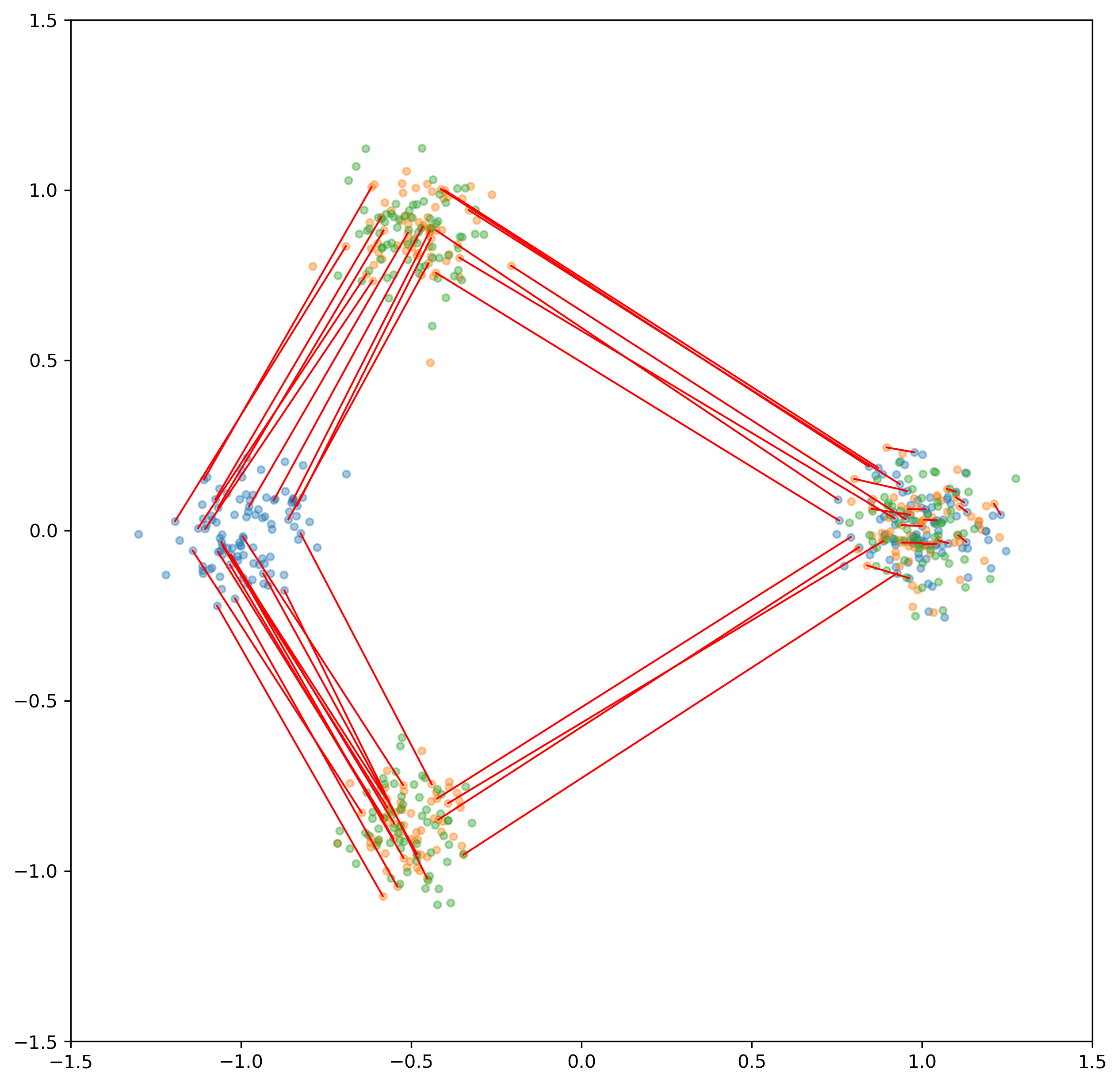
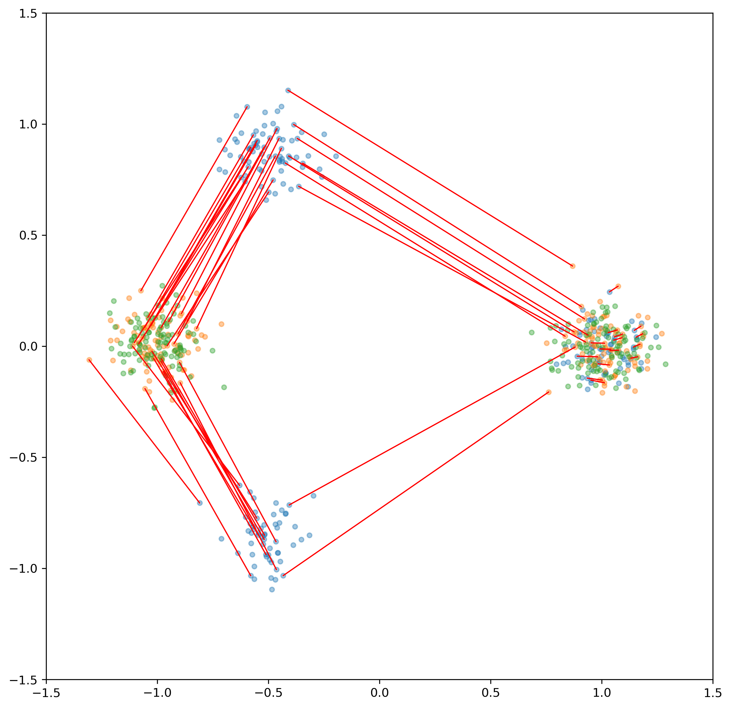
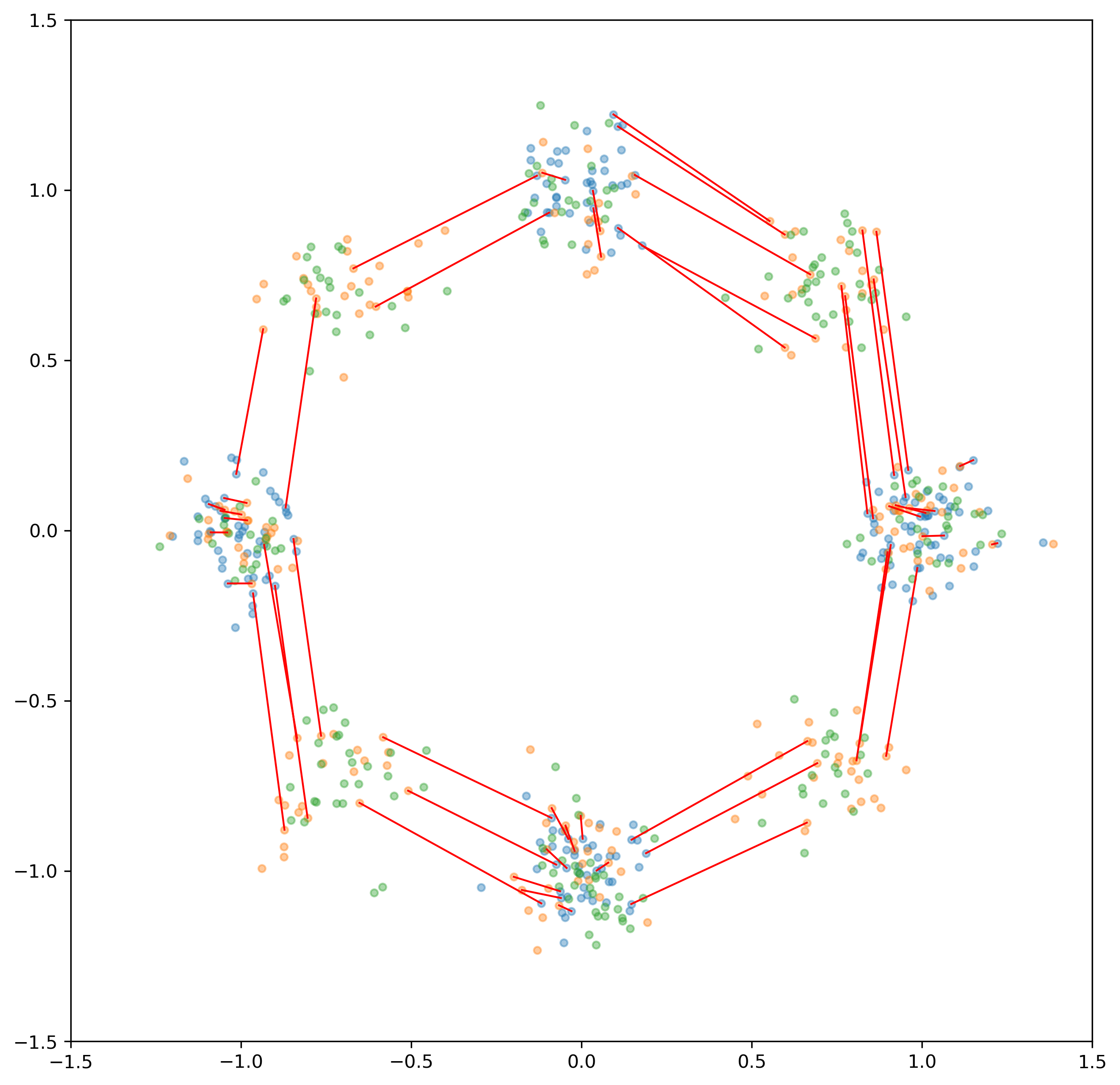
Figure 1: $m$-Gaussian mixture transferred with KRDA to an $n$-Gaussian mixture; we plot the source (blue), target (green), transferred (orange) and some mappings (red).

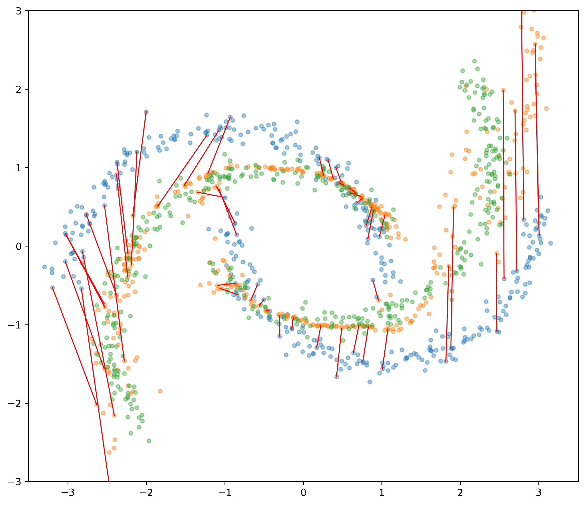
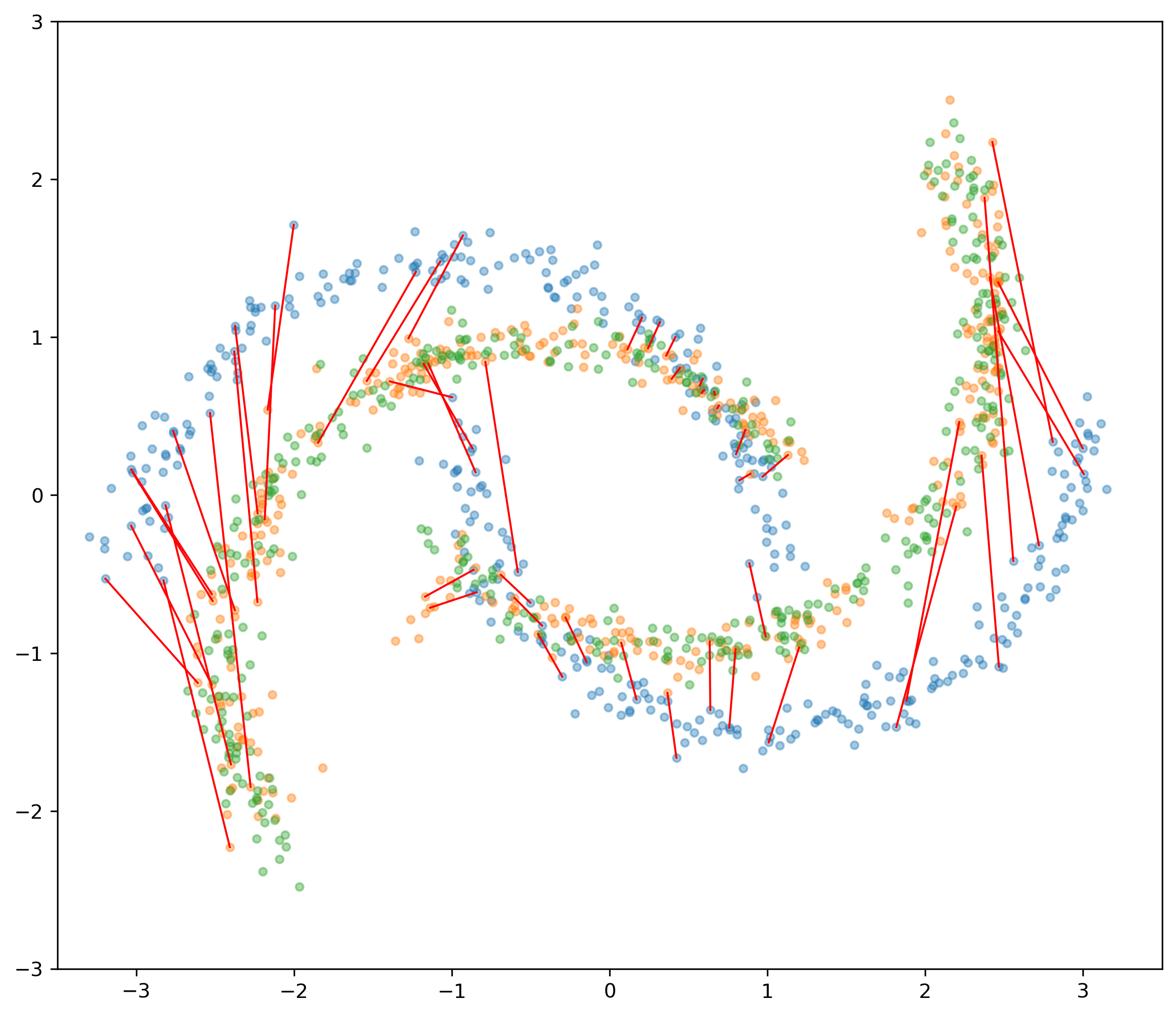
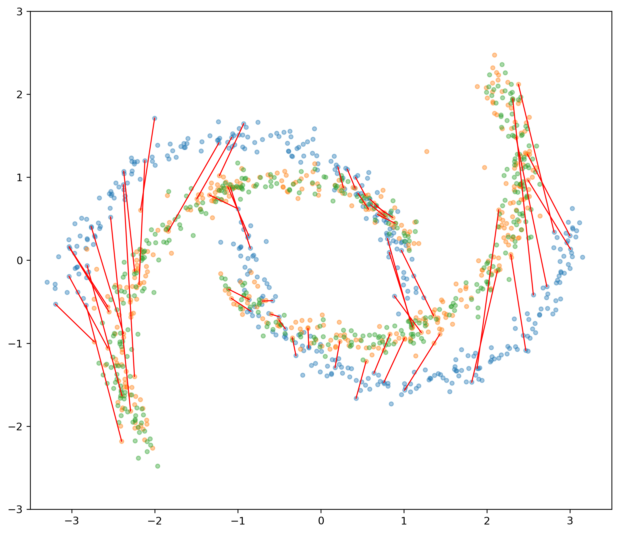
2 components	3 components	5 components

Figure 2: KRDA on the inter-twinning moon dataset with different number of components; we plot the source (blue), target (green), transferred (orange) and some mappings (red).

Limitations

KRDA has two main limitations. The first one is the reliance of KRDA on the estimation made by RNADE. Since RNADE does not generalize well to high-dimensional spaces ($\geq 100$), we cannot expect KRDA to work well in this regime. The second limitation is the computation cost of the transfer: the algorithm iterates on the dataset (parallelizable) and on the components (not parallelizable because of the conditional distributions). Even though KRDA is linear in the number of samples, it may not be suited for very large datasets of millions of samples. As we do not use label information, our approach is suited for the covariate-shift setting.

6 Experiments

6.1 Domain adaptation

In this section, we evaluate KRDA in both synthetic and real data sets. In all KRDA experiments, we model the source and target distributions with mixtures of five Gaussian components. All the following experiments are performed in the unsupervised domain adaptation setting, when no labels of the target domain are accessible. After transformation, we apply an SVM on the transferred source. We compare our method to various techniques which can be classified into three classes:

• Baseline solutions: For a specific ML model, here Support Vector Machine (SVM), Source only learns this model using source data set with its labels; Target only learns the model by using the labeled target data (note that none of the transfer competitors have access the target data set labels, so this is meant as an optimistic baseline);

• Shallow solutions: Subspace Alignment SA, (Fernando et al., 2013) and reweighting methods Transfer Component Analysis TCA (Pan et al., 2011), Kernel Mean Matching KMM(Gretton et al., 2009) , each followed by a SVM;

• Optimal Transport OT (Courty et al., 2017), followed by a SVM;

• Deep learning solutions include DAN (Long et al., 2015), DANN (Ganin et al., 2016), JAN (Long et al., 2017), CDAN (Long et al., 2018) and SHOT (Liang et al., 2020). We implement DAN, DANN, JAN and CDAN using the dalib library (Junguang Jiang, 2020). Instead of using the original image classifier in dalib that would be unsuitable in our benchmark, we use a five-layer MLP for each algorithm. For SHOT, the feature net is a four-layer MLP and the classifier net is a one-layer regression model a total of five layers.

For space reasons, we only show a sub-selection of the benchmark: the complete tables are located in Appendix A.

Hyperparameter Tuning

We fix most hyperparameters in our experiments. In deep learning models (DANN, JAN, and CDAN) $\eta=1$. The number of hidden neurons of MLP is set to 250 which will be equivalent to the number of parameters of the KRDA models. All the deep learning models are trained using the Adam optimizer (Kingma and Ba, 2015) with a learning rate set to $10^{-3}$.

Metric and cross validation

Accuracy is used as the metric to evaluate the performance of different algorithms in the following experiments. All experiments have two classes. We run each experiment five times. In each running, we randomly pick 90% source and 90% target data to train the model. The test is systematically performed on unseen samples from the target data set. In each table, we report the average accuracy of the five experiments as well as 95% confidence intervals. The code used in all our experiments is available on Github.

6.2 Synthetic data experiments

Mixtures of Gaussians

We generate a mixture of Gaussians for the source and target data. We use 1000 samples in both data sets, and we are interested in seeing how the domain adaptation tasks are handled by KRDA. For all tasks, RNADE uses $N=5$ Gaussian components and a hidden layer of dimension $50$. We plot several transfers from mixtures of $m$ Gaussians to mixtures of $n$ Gaussians. The results are presented in Figure 1.

Inter-twinning moons

We perform three experiments on the classical inter-twinning moons dataset. In all these experiments, KRDA uses $N=5$ Gaussian components and a hidden layer of dimension $50$. The inter-twinning moon dataset is composed of two interlacing half-moons with labels $0$ and $1$.

1. We show the KRDA embedding from the source to a target domain with different components of the Gaussian mixture. We highlight the transfer of the same set of source sample in all figures. Both train and target data are of size $1000$, the target distribution is a $40^{\circ}$ rotation of the source distribution. These visualizations are shown in Figure 2.

2. We use the same experimental setup as in (Germain et al., 2013). We sample $300$ samples from the source distribution and $300$ in the target domain with various angles between $10^{\circ}$ and $90^{\circ}$. The difficulty of the problem increases with the angle. The test set is composed of $1000$ samples from the target distribution. We show the performance of KRDA and competitors in Table 4.

3. KRDA is run in six inter-twining moons tasks to investigate its performance in different training sizes. The source and target training data size ranges from $200$ to $1,000$. In each task, the target data distribution is rotated with $40^{\circ}$ from the source. Following previous cross validation setting, in each task we run each algorithm five times with randomly picked 90% source and 90% target data and average the results. Figure 3 shows results and the corresponding 95% confidence interval. We find that although all algorithms tend to converge, KRDA acts excellently in small size cases and it is stabler than other algorithms in the low-data setting.

Table 1: Inter-twinning moons unsupervised

Task	Source	Target	DANN	SA	KMM	OT	SHOT	KRDA
$10^{\circ}$	100$\pm$0.00	100$\pm$0	100$\pm$0.00	85.3$\pm$0.5	50.1$\pm$12.0	100.0$\pm$0.0	82.8$\pm$10.8	100$\pm$0.0
$20^{\circ}$	99.9$\pm$0.1	100$\pm$0	99.3$\pm$0.5	78.5$\pm$0.4	53.0$\pm$8.8	100.0$\pm$0.0	81.4$\pm$3.7	100$\pm$0.0
$30^{\circ}$	96.6$\pm$0.4	100$\pm$0	89.4$\pm$7.2	73.4$\pm$0.3	51.4$\pm$10.9	99.8$\pm$0.2	77.1$\pm$2.1	100$\pm$0.0
$40^{\circ}$	73.1$\pm$2.5	100$\pm$0	73.8$\pm$21.3	69.2$\pm$0.2	53.4$\pm$27.3	89.6$\pm$1.2	24.4$\pm$2.2	98.4$\pm$2.2
$50^{\circ}$	41.5$\pm$2.0	100$\pm$0	48.5$\pm$21.9	61.8$\pm$0.5	56.3$\pm$7.8	83.8$\pm$0.8	22.3$\pm$1.6	98.4$\pm$1.5
$60^{\circ}$	28.7$\pm$0.6	100$\pm$0	44.2$\pm$14.3	54.8$\pm$0.4	47.8$\pm$18.1	78.0$\pm$1.3	19.9$\pm$1.3	90.5$\pm$2.8
$70^{\circ}$	23.3$\pm$0.4	100$\pm$0	24.3$\pm$1.6	49.0$\pm$0.4	52.5$\pm$9.0	71.6$\pm$0.6	17.4$\pm$1.2	84.4$\pm$0.8
$80^{\circ}$	20.4$\pm$1.70	100$\pm$0	20.1$\pm$2.4	43.2$\pm$0.6	48.2$\pm$9.1	65.8$\pm$0.7	15.7$\pm$1.3	81.2$\pm$3.4
$90^{\circ}$	18.1$\pm$0.3	100$\pm$0	17.7$\pm$1.5	38.2$\pm$0.1	54.4$\pm$17.9	59.4$\pm$1.2	14.8$\pm$1.3	71.1$\pm$3.9

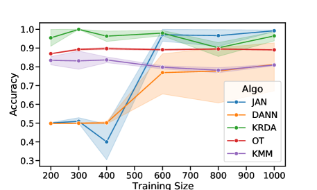
Figure 3: The learning curves of different UDA algorithms under different source and target training sizes. KRDA has excellent performance on small data sets and it shows very stable accuracy over different training sizes.

6.3 Experiments on real data

Hepmass

The HEPMASS data comes from high-energy physics (Baldi et al., 2016). The objective of the task is to learn how to separate exotic particles from background noise using collision data (27 measured features). The data may be split according to the mass of the observed particles ($m\in\{500,750,1000,1250,1500\}$). We create different transfer learning tasks: transferring the domain from one mass to another. We build the source and target data by subsampling $1000$ and $500$ instances from the original data with a given source and target mass, respectively. We also sample $2000$ independent instances from the target domain for the test set. KRDA uses $N=5$ Gaussian components and dimension $100$ for its hidden layer. Each transfer of the source data is followed by a SVM with the hyperparameters shared for all experiments that require it. SA uses $10$ components. The results are summarized in Table 5. As shown, KRDA performs similarly and often better than state-of-the-art competitors.

Table 2: HEPMASS unsupervised domain adaptation

Task	Source	Target	DANN	SA	KMM	OT	SHOT	KRDA
500 $\to$750	68.7$\pm$0.1	82.2$\pm$0.3	56.7$\pm$2.9	67.9$\pm$1.2	60.7$\pm$3.5	67.6$\pm$2.0	74.1$\pm$1.9	75.6$\pm$2.3
500 $\to$1000	67.2$\pm$0.1	89.2$\pm$0.4	56.7$\pm$4.4	71.7$\pm$1.0	50.1$\pm$10.8	72.1$\pm$1.9	85.5$\pm$1.1	80.3$\pm$3.1
500 $\to$1250	62.6$\pm$0.3	93.3$\pm$0.3	54.3$\pm$3.8	71.3$\pm$4.1	40.1$\pm$17.9	74.6$\pm$2.3	89.8$\pm$1.4	82.9$\pm$3.5
500 $\to$1500	58.0$\pm$0.2	95.4$\pm$0.4	55.7$\pm$3.1	72.0$\pm$3.7	61.8$\pm$20.9	73.6$\pm$3.0	90.8$\pm$0.4	80.0$\pm$6.1
750 $\to$500	52.6$\pm$0.1	56.3$\pm$0.5	54.0$\pm$0.2	56.1$\pm$1.1	53.1$\pm$0.5	56.9$\pm$0.7	53.4$\pm$0.8	55.7$\pm$1.1
750 $\to$1000	86.5$\pm$0.1	89.2$\pm$0.4	82.2$\pm$0.8	83.1$\pm$2.6	87.9$\pm$0.2	86.2$\pm$0.6	87.5$\pm$0.6	87.7$\pm$0.7
750 $\to$1250	87.7$\pm$0.0	95.4$\pm$0.4	81.3$\pm$2.9	88.2$\pm$3.1	89.5$\pm$0.5	92.5$\pm$0.9	92.0$\pm$0.4	92.3$\pm$1.3
750 $\to$1500	87.7$\pm$0.0	95.4$\pm$0.4	82.5$\pm$2.8	88.2$\pm$3.1	89.5$\pm$0.5	92.5$\pm$0.9	91.7$\pm$0.4	92.8$\pm$1.6
1000 $\to$500	51.9$\pm$0.0	56.3$\pm$0.5	51.9$\pm$0.4	55.5$\pm$0.9	51.9$\pm$0.2	55.0$\pm$0.5	53.3$\pm$0.4	53.2$\pm$1.7
1000 $\to$750	77.1$\pm$0.1	82.2$\pm$0.3	74.8$\pm$0.6	77.3$\pm$1.1	77.7$\pm$0.4	80.5$\pm$0.6	80.6$\pm$1.1	80.7$\pm$0.9
1000 $\to$1250	92.6$\pm$0.0	93.3$\pm$0.3	90.9$\pm$0.5	88.7$\pm$1.0	91.2$\pm$0.4	92.1$\pm$0.4	91.7$\pm$0.4	92.5$\pm$0.3
1000 $\to$1500	93.0$\pm$0.0	95.4$\pm$0.4	91.0$\pm$0.6	88.3$\pm$2.4	91.2$\pm$0.3	93.5$\pm$0.6	92.0$\pm$0.3	93.9$\pm$0.9
1250 $\to$500	51.3$\pm$0.0	56.3$\pm$0.5	51.5$\pm$0.4	55.7$\pm$0.9	52.1$\pm$0.5	53.8$\pm$0.5	53.5$\pm$0.5	56.5$\pm$1.4
1250 $\to$750	68.9$\pm$0.1	82.2$\pm$0.3	70.2$\pm$1.2	77.0$\pm$1.0	77.0$\pm$0.7	80.1$\pm$0.3	77.8$\pm$0.9	80.2$\pm$0.7
1250 $\to$1000	87.7$\pm$0.1	89.2$\pm$0.4	84.7$\pm$0.5	82.7$\pm$2.4	88.6$\pm$0.5	88.4$\pm$0.7	87.4$\pm$0.7	88.5$\pm$0.5
1250 $\to$1500	94.1$\pm$0.1	95.4$\pm$0.4	93.0$\pm$0.3	89.5$\pm$2.4	92.7$\pm$0.1	94.3$\pm$0.4	94.0$\pm$0.2	94.0$\pm$0.7
1500 $\to$500	50.8$\pm$0.1	56.3$\pm$0.5	50.6$\pm$0.5	56.2$\pm$0.6	51.8$\pm$0.2	53.2$\pm$0.5	51.8$\pm$0.4	54.0$\pm$2.2
1500 $\to$750	63.3$\pm$0.1	82.2$\pm$0.3	64.3$\pm$1.2	78.2$\pm$1.6	75.0$\pm$0.6	80.0$\pm$0.2	76.4$\pm$0.8	80.4$\pm$1.2
1500 $\to$1000	83.9$\pm$0.1	89.2$\pm$0.4	82.8$\pm$0.7	84.7$\pm$1.8	88.4$\pm$0.4	87.4$\pm$0.4	88.9$\pm$0.4	88.5$\pm$0.8
1500 $\to$1250	92.9$\pm$0.1	93.3$\pm$0.3	90.6$\pm$0.5	88.7$\pm$2.3	93.0$\pm$0.3	92.1$\pm$0.5	92.6$\pm$0.2	92.4$\pm$0.8

Amazon dataset

This data (McAuley et al., 2015) is an aggregation of reviews from four different products (dvd (D), books (B), electronics (E), kitchen (K)) and their given grade by customers. Each product or domain has about $2000$ training samples and $4000$ test samples. Each sample is presented by $5000$ features and is associated to a binary class: $0$ for samples ranked less than three stars and $1$ otherwise. The goal is to transfer the review-to-grade classification from one product to another. Thus we created twelve transfer tasks using these products. As KRDA is based on RNADE for the density estimation, and RNADE is not designed for high dimensional data, we used a neural net (NN) to reduce the sample dimensionality from $5000$ to $5$. The NN has two hidden layers of dimensions 10 and 5 (the encoding dimension). For each task, we train the NN as a classifier on the source data with a cross entropy loss. We then cut the output layer and use the trained NN to encode both the source and target data into $5$ dimensions. This dimension reduction is the input data of all the algorithms on the benchmark and we trained all the competitors on this data. The results are shown in Table 6.

Table 3: Amazon dataset, unsupervised. Tasks are B: books, D: Dvd, E: Electronics, K: kitchen

Task	Source	Target	DANN	SA	KMM	OT	SHOT	KRDA
B $\to$ D	79.9$\pm$0.1	79.4$\pm$0.1	79.9$\pm$0.1	79.9 $\pm$ 0.1	79.9$\pm$0.1	79.7$\pm$0.1	79.7$\pm$0.6	80.0$\pm$0.2
B $\to$ E	69.2$\pm$0.2	72.7$\pm$0.0	69.9$\pm$0.4	73.0 $\pm$ 0.1	71.8$\pm$0.1	73.0$\pm$0.1	72.6$\pm$0.7	73.0$\pm$0.1
B $\to$ K	75.7$\pm$0.2	76.2$\pm$0.1	75.8$\pm$0.2	76.1 $\pm$ 0.1	76.3$\pm$0.1	76.2$\pm$0.1	76.2$\pm$0.2	76.2$\pm$0.1
D $\to$ B	75.1$\pm$0.1	75.6$\pm$0.1	75.1$\pm$0.2	75.3 $\pm$ 0.1	75.5$\pm$0.1	75.2$\pm$0.1	75.5$\pm$0.1	75.3$\pm$0.1
D $\to$ E	71.0$\pm$0.3	74.6$\pm$0.1	71.1$\pm$0.7	74.3 $\pm$ 0.1	72.7$\pm$0.2	74.6$\pm$0.1	73.8$\pm$0.9	74.4$\pm$0.2
D $\to$ K	74.9$\pm$0.1	77.3$\pm$0.1	74.8$\pm$0.5	77.5 $\pm$ 0.1	76.2$\pm$0.1	77.5$\pm$0.1	77.0$\pm$0.5	76.3$\pm$0.2
E $\to$ B	70.7$\pm$0.1	71.5$\pm$0.0	70.6$\pm$0.4	71.2 $\pm$ 0.2	70.9$\pm$0.2	71.1$\pm$0.1	71.3$\pm$0.3	70.9$\pm$0.2
E $\to$ D	72.3$\pm$0.1	73.6$\pm$0.0	72.1$\pm$0.4	73.1 $\pm$ 0.2	73.3$\pm$0.4	72.7$\pm$0.1	72.8$\pm$0.3	72.6$\pm$0.5
E $\to$ K	86.1$\pm$0.1	86.2$\pm$0.1	85.5$\pm$0.5	85.8 $\pm$ 0.2	83.5$\pm$0.3	86.0$\pm$0.1	85.6$\pm$0.6	85.2$\pm$1.0
K $\to$ B	71.2$\pm$0.2	71.4$\pm$0.1	71.2$\pm$0.3	71.6 $\pm$ 0.1	71.7$\pm$0.1	71.8$\pm$0.0	71.6$\pm$0.1	69.4$\pm$0.3
K $\to$ D	70.8$\pm$0.1	72.8$\pm$0.0	70.7$\pm$1.1	72.7 $\pm$ 0.3	70.6$\pm$0.0	72.8$\pm$0.2	70.6$\pm$1.0	72.8$\pm$0.7
K $\to$ E	84.0$\pm$0.0	84.4$\pm$0.0	84.0$\pm$0.2	84.3 $\pm$ 0.0	84.2$\pm$0.0	84.3$\pm$0.0	84.2$\pm$0.1	84.1$\pm$0.1

7 Conclusion

In this paper, we presented a novel transfer learning framework that exploits recent advances in density estimation techniques in order to transfer samples from a source domain to a target domain with a distribution shift using Knothe-Rosenblatt transport. The property that is invariant by the transfer performed by KRDA is the one dimensional conditional quantile distributions from the source in the target domain space, using an autoregressive setup. We showed that KRDA is state of the art on small to moderate dimensional tasks, often outperforming competitors especially in the case where there are few data samples.

Future work includes extending KRDA to the semi-supervised domain adaptation where a few labels are present in the target data. Another interesting research direction is to use other modern density estimators such as normalizing flows or variational autoencoders, in place of autoregressive mixture density nets.

 

Knothe-Rosenblatt transport for Unsupervised Domain Adaptation
 

Supplementary material

Appendix A Experiments

A.1 Inter-twinning moons

Table 4: Inter-twinning moons unsupervised

Task	Source	Target	CDAN	DAN	JAN	TCA	KRDA
$10^{\circ}$	100$\pm$0	100$\pm$0	100$\pm$0	50.0$\pm$0.1	100$\pm$0	100.0$\pm$0	100$\pm$0
$20^{\circ}$	99.9$\pm$0.1	100$\pm$0	99.8$\pm$0.2	48.5$\pm$3.4	100$\pm$0	100.0$\pm$0	100$\pm$0
$30^{\circ}$	96.6$\pm$0.40	100$\pm$0	97.8$\pm$2.1	56.1$\pm$13.7	99.7$\pm$0.7	100.0$\pm$0	100$\pm$0
$40^{\circ}$	73.1$\pm$2.50	100$\pm$0	80.4$\pm$14.4	50.0$\pm$0.1	93.2$\pm$7.9	98.0$\pm$0.8	98.4$\pm$2.2
$50^{\circ}$	41.5$\pm$2.0	100$\pm$0	47.4$\pm$24.5	50.0$\pm$0.1	89.8$\pm$4.3	80.1$\pm$2.0	98.4$\pm$1.5
$60^{\circ}$	28.7$\pm$0.6	100$\pm$0	30.1$\pm$5.0	50.0$\pm$0.1	87.4$\pm$4.3	44.8$\pm$4.7	90.5$\pm$2.8
$70^{\circ}$	23.3$\pm$0.4	100$\pm$0	24.9$\pm$1.7	49.9$\pm$0	62.2$\pm$34.9	24.9$\pm$0.6	84.4$\pm$0.8
$80^{\circ}$	20.4$\pm$1.7	100$\pm$0	26.7$\pm$10.4	50.0$\pm$0.1	49.9$\pm$22.6	20.5$\pm$0.2	81.2$\pm$3.4
$90^{\circ}$	18.1$\pm$0.3	100$\pm$0	17.2$\pm$0.7	50.0$\pm$0.1	27.9$\pm$14.1	17.8$\pm$0.4	71.1$\pm$3.9

A.2 Hepmass

Table 5: HEPMASS unsupervised domain adaptation

solution	Source	Target	CDAN	DAN	JAN	TCA	KRDA
500 $\to$750	68.7$\pm$0.1	82.2$\pm$0.3	56.0$\pm$4.0	51.3$\pm$0.7	58.2$\pm$1.9	67.2$\pm$0.4	75.6$\pm$2.3
500 $\to$1000	67.2$\pm$0.1	89.2$\pm$0.4	49.2$\pm$5.6	51.4$\pm$4.1	56.1$\pm$3.8	71.7$\pm$0.4	80.3$\pm$3.1
500 $\to$1250	62.6$\pm$0.3	93.3$\pm$0.3	53.7$\pm$8.8	48.9$\pm$2.7	54.9$\pm$2.3	77.9$\pm$0.3	82.9$\pm$3.5
500 $\to$1500	58.0$\pm$0.2	95.4$\pm$0.4	56.3$\pm$9.1	52.8$\pm$0.3	54.3$\pm$2.6	75.9$\pm$0.5	80.0$\pm$6.1
750 $\to$500	52.6$\pm$0.1	56.3$\pm$0.5	54.2$\pm$0.5	50.4$\pm$0.8	54.9$\pm$0.9	53.7$\pm$0.2	55.7$\pm$1.1
750 $\to$1000	86.5$\pm$0.1	89.2$\pm$0.4	82.6$\pm$0.4	49.0$\pm$0.2	81.8$\pm$1.7	84.5$\pm$0.2	87.7$\pm$0.7
750 $\to$1250	87.7$\pm$0.0	95.4$\pm$0.4	82.5$\pm$3.1	52.1$\pm$7.4	77.8$\pm$3.9	85.7$\pm$0.1	92.3$\pm$1.3
750 $\to$1500	87.7$\pm$0.0	95.4$\pm$0.4	74.8$\pm$7.9	56.1$\pm$11.8	76.6$\pm$2.1	85.7$\pm$0.1	92.8$\pm$1.6
1000 $\to$500	51.9$\pm$0.0	56.3$\pm$0.5	52.0$\pm$0.5	50.0$\pm$0.0	51.2$\pm$0.6	53.1$\pm$0.1	53.2$\pm$1.7
1000 $\to$750	77.1$\pm$0.1	82.2$\pm$0.3	74.8$\pm$1.2	51.5$\pm$0.0	76.2$\pm$1.1	73.6$\pm$0.2	80.7$\pm$0.9
1000 $\to$1250	92.6$\pm$0.0	93.3$\pm$0.3	91.2$\pm$0.5	57.2$\pm$17.3	88.8$\pm$0.4	91.1$\pm$0.1	92.5$\pm$0.3
1000 $\to$1500	93.0$\pm$0.0	95.4$\pm$0.4	90.6$\pm$0.6	61.4$\pm$17.0	88.6$\pm$1.3	91.7$\pm$0.1	93.9$\pm$0.9
1250 $\to$500	51.3$\pm$0.0	56.3$\pm$0.5	51.3$\pm$0.3	50.0$\pm$0.0	52.1$\pm$0.6	51.7$\pm$0.1	56.5$\pm$1.4
1250 $\to$750	68.9$\pm$0.1	82.2$\pm$0.3	69.8$\pm$0.9	54.8$\pm$12.6	76.8$\pm$0.7	69.8$\pm$0.2	80.2$\pm$0.7
1250 $\to$1000	87.7$\pm$0.1	89.2$\pm$0.4	85.2$\pm$0.3	69.9$\pm$19.1	85.3$\pm$0.7	86.5$\pm$0.2	88.5$\pm$0.5
1250 $\to$1500	94.1$\pm$0.1	95.4$\pm$0.4	93.2$\pm$0.4	72.6$\pm$23.8	93.3$\pm$0.7	93.0$\pm$0.1	94.0$\pm$0.7
1500 $\to$500	50.8$\pm$0.1	56.3$\pm$0.5	50.2$\pm$0.4	50.0$\pm$0.2	51.3$\pm$0.6	51.3$\pm$0.1	54.0$\pm$2.2
1500 $\to$750	63.3$\pm$0.1	82.2$\pm$0.3	62.1$\pm$0.9	53.1$\pm$10.3	73.9$\pm$0.6	66.0$\pm$0.2	80.4$\pm$1.2
1500 $\to$1000	83.9$\pm$0.1	89.2$\pm$0.4	82.3$\pm$1.4	75.8$\pm$11.5	85.9$\pm$1.7	83.4$\pm$0.2	88.5$\pm$0.8
1500 $\to$1250	92.9$\pm$0.1	93.3$\pm$0.3	91.0$\pm$0.6	84.1$\pm$18.8	91.3$\pm$0.2	91.9$\pm$0.3	92.4$\pm$0.8

A.3 Amazon

Table 6: Amazon dataset, unsupervised. Tasks are B: books, D: Dvd, E: Electronics, K: kitchen

solution	Source	Target	CDAN	DAN	JAN	TCA	KRDA
B $\to$ D	79.9$\pm$0.1	79.4$\pm$0.1	79.7$\pm$0.6	63.1$\pm$15.5	59.5$\pm$13.5	79.9$\pm$0.1	80.0$\pm$0.2
B $\to$ E	69.2$\pm$0.2	72.7$\pm$0.0	64.5$\pm$8.5	59.6$\pm$10.8	70.9$\pm$0.4	69.9$\pm$0.2	73.0$\pm$0.1
B $\to$ K	75.7$\pm$0.2	76.2$\pm$0.1	75.8$\pm$0.1	55.2$\pm$11.6	70.9$\pm$11.5	75.8$\pm$0.1	76.2$\pm$0.1
D $\to$ B	75.1$\pm$0.1	75.6$\pm$0.1	75.3$\pm$0.2	69.3$\pm$9.1	70.2$\pm$10.9	75.0$\pm$0.0	75.3$\pm$0.1
D $\to$ E	71.0$\pm$0.3	74.6$\pm$0.1	66.9$\pm$9.3	68.0$\pm$9.9	67.0$\pm$9.9	71.2$\pm$0.2	74.4$\pm$0.2
D $\to$ K	74.9$\pm$0.1	77.3$\pm$0.1	75.1$\pm$0.2	60.2$\pm$14.0	62.1$\pm$13.0	75.3$\pm$0.0	76.3$\pm$0.2
E $\to$ B	70.7$\pm$0.1	71.5$\pm$0.0	70.7$\pm$0.4	58.3$\pm$11.7	58.6$\pm$11.5	71.0$\pm$0.1	70.9$\pm$0.2
E $\to$ D	72.3$\pm$0.1	73.6$\pm$0.0	71.4$\pm$1.3	66.5$\pm$9.8	63.8$\pm$12.6	72.1$\pm$0.1	72.6$\pm$0.5
E $\to$ K	86.1$\pm$0.1	86.2$\pm$0.1	85.5$\pm$0.4	83.5$\pm$5.4	64.4$\pm$19.6	86.0$\pm$0.2	85.2$\pm$1.0
K $\to$ B	71.2$\pm$0.2	71.4$\pm$0.1	71.2$\pm$0.2	69.7$\pm$3.6	62.6$\pm$11.6	71.2$\pm$0.1	69.4$\pm$0.3
K $\to$ D	70.8$\pm$0.1	72.8$\pm$0.0	70.5$\pm$0.4	62.4$\pm$11.7	71.0$\pm$0.2	70.7$\pm$0.0	72.8$\pm$0.7
K $\to$ E	84.0$\pm$0.0	84.4$\pm$0.0	84.0$\pm$0.2	84.1$\pm$0.2	77.2$\pm$15.4	83.9$\pm$0.1	84.1$\pm$0.1

References

- (1)
- Arjoune and Faruque (2020) Arjoune, Y. and Faruque, S. (2020). Artificial intelligence for 5g wireless systems: Opportunities, challenges, and future research direction. In 2020 10th Annual Computing and Communication Workshop and Conference (CCWC), pages 1023–1028. IEEE.
- Baldi et al. (2016) Baldi, P., Cranmer, K., Faucett, T., Sadowski, P., and Whiteson, D. (2016). Parameterized neural networks for high-energy physics. The European Physical Journal C, 76.
- Benzaid and Taleb (2020) Benzaid, C. and Taleb, T. (2020). Ai-driven zero touch network and service management in 5g and beyond: Challenges and research directions. IEEE Network, 34(2):186–194.
- Bishop (1994) Bishop, C. M. (1994). Mixture density networks. Technical report, Birmingham.
- Carlier et al. (2009) Carlier, G., Galichon, A., and Santambrogio, F. (2009). From knothe’s transport to brenier’s map and a continuation method for optimal transport. SIAM J. Math. Anal., 41:2554–2576.
- Courty et al. (2017) Courty, N., Flamary, R., Tuia, D., and Rakotomamonjy, A. (2017). Optimal transport for domain adaptation. IEEE Transactions on Pattern Analysis and Machine Intelligence, 39(9):1853–1865.
- Donahue et al. (2013) Donahue, J., Hoffman, J., Rodner, E., Saenko, K., and Darrell, T. (2013). Semi-supervised domain adaptation with instance constraints. In 2013 IEEE Conference on Computer Vision and Pattern Recognition, pages 668–675.
- Fernando et al. (2013) Fernando, B., Habrard, A., Sebban, M., and Tuytelaars, T. (2013). Unsupervised visual domain adaptation using subspace alignment. In Proceedings of the IEEE international conference on computer vision, pages 2960–2967.
- Fu et al. (2018) Fu, Y., Wang, S., Wang, C.-X., Hong, X., and McLaughlin, S. (2018). Artificial intelligence to manage network traffic of 5g wireless networks. IEEE Network, 32(6):58–64.
- Ganin et al. (2016) Ganin, Y., Ustinova, E., Ajakan, H., Germain, P., Larochelle, H., Laviolette, F., March, M., and Lempitsky, V. (2016). Domain-adversarial training of neural networks. Journal of Machine Learning Research, 17(59):1–35.
- Germain et al. (2013) Germain, P., Habrard, A., Laviolette, F., and Morvant, E. (2013). A pac-bayesian approach for domain adaptation with specialization to linear classifiers. In Dasgupta, S. and McAllester, D., editors, Proceedings of the 30th International Conference on Machine Learning, volume 28 of Proceedings of Machine Learning Research, pages 738–746, Atlanta, Georgia, USA. PMLR.
- Gong et al. (2012) Gong, B., Shi, Y., Sha, F., and Grauman, K. (2012). Geodesic flow kernel for unsupervised domain adaptation. In 2012 IEEE Conference on Computer Vision and Pattern Recognition, pages 2066–2073. IEEE.
- Gong et al. (2016) Gong, M., Zhang, K., Liu, T., Tao, D., Glymour, C., and Schölkopf, B. (2016). Domain adaptation with conditional transferable components. In International conference on machine learning, pages 2839–2848.
- Gretton et al. (2007) Gretton, A., Borgwardt, K., Rasch, M., Schölkopf, B., and Smola, A. J. (2007). A kernel method for the two-sample-problem. In Advances in neural information processing systems, pages 513–520.
- Gretton et al. (2009) Gretton, A., Smola, A., Huang, J., Schmittfull, M., Borgwardt, K., and Schölkopf, B. (2009). Covariate shift by kernel mean matching. Dataset shift in machine learning, 3(4):5.
- Ho et al. (2019) Ho, J., Chen, X., Srinivas, A., Duan, Y., and Abbeel, P. (2019). Flow++: Improving flow-based generative models with variational dequantization and architecture design. volume 97 of Proceedings of Machine Learning Research, pages 2722–2730, Long Beach, California, USA. PMLR.
- Huang et al. (2007) Huang, J., Gretton, A., Borgwardt, K., Schölkopf, B., and Smola, A. J. (2007). Correcting sample selection bias by unlabeled data. In Advances in neural information processing systems, pages 601–608.
- Junguang Jiang (2020) Junguang Jiang, Bo Fu, M. L. (2020). Transfer-learning-library. https://github.com/thuml/Transfer-Learning-Library.
- Kégl et al. (2021) Kégl, B., Hurtado, G., and Thomas, A. (2021). Model-based micro-data reinforcement learning: what are the crucial model properties and which model to choose? In International Conference on Learning Representations.
- Kingma and Ba (2015) Kingma, D. P. and Ba, J. (2015). Adam: A method for stochastic optimization. In Bengio, Y. and LeCun, Y., editors, 3rd International Conference on Learning Representations, ICLR 2015, San Diego, CA, USA, May 7-9, 2015, Conference Track Proceedings.
- Knothe (1957) Knothe, H. (1957). Contributions to the theory of convex bodies. Michigan Mathematical Journal, 4(1):39 – 52.
- Kouw and Loog (2019) Kouw, W. M. and Loog, M. (2019). A review of domain adaptation without target labels. IEEE transactions on pattern analysis and machine intelligence.
- Larochelle and Murray (2011) Larochelle, H. and Murray, I. (2011). The neural autoregressive distribution estimator. volume 15 of Proceedings of Machine Learning Research, pages 29–37, Fort Lauderdale, FL, USA. JMLR Workshop and Conference Proceedings.
- Li et al. (2020a) Li, R., Jiao, Q., Cao, W., Wong, H.-S., and Wu, S. (2020a). Model adaptation: Unsupervised domain adaptation without source data. In Proceedings of the IEEE/CVF Conference on Computer Vision and Pattern Recognition, pages 9641–9650.
- Li et al. (2020b) Li, X., Grandvalet, Y., Davoine, F., Cheng, J., Cui, Y., Zhang, H., Belongie, S., Tsai, Y.-H., and Yang, M.-H. (2020b). Transfer learning in computer vision tasks: Remember where you come from. Image and Vision Computing, 93:103853.
- Liang et al. (2020) Liang, J., Hu, D., and Feng, J. (2020). Do we really need to access the source data? source hypothesis transfer for unsupervised domain adaptation. In International Conference on Machine Learning, pages 6028–6039. PMLR.
- Long et al. (2015) Long, M., Cao, Y., Wang, J., and Jordan, M. (2015). Learning transferable features with deep adaptation networks. In International conference on machine learning, pages 97–105. PMLR.
- Long et al. (2018) Long, M., CAO, Z., Wang, J., and Jordan, M. I. (2018). Conditional adversarial domain adaptation. In Bengio, S., Wallach, H., Larochelle, H., Grauman, K., Cesa-Bianchi, N., and Garnett, R., editors, Advances in Neural Information Processing Systems, volume 31, pages 1640–1650. Curran Associates, Inc.
- Long et al. (2017) Long, M., Zhu, H., Wang, J., and Jordan, M. I. (2017). Deep transfer learning with joint adaptation networks. In Precup, D. and Teh, Y. W., editors, Proceedings of the 34th International Conference on Machine Learning, volume 70 of Proceedings of Machine Learning Research, pages 2208–2217, International Convention Centre, Sydney, Australia. PMLR.
- Malte and Ratadiya (2019) Malte, A. and Ratadiya, P. (2019). Evolution of transfer learning in natural language processing.
- McAuley et al. (2015) McAuley, J., Targett, C., Shi, Q., and van den Hengel, A. (2015). Image-based recommendations on styles and substitutes. SIGIR ’15, page 43–52, New York, NY, USA. Association for Computing Machinery.
- Muzellec and Cuturi (2019) Muzellec, B. and Cuturi, M. (2019). Subspace detours: Building transport plans that are optimal on subspace projections. In NeurIPS.
- Oord et al. (2016) Oord, A. V., Kalchbrenner, N., and Kavukcuoglu, K. (2016). Pixel recurrent neural networks. volume 48 of Proceedings of Machine Learning Research, pages 1747–1756, New York, New York, USA. PMLR.
- Pan et al. (2010) Pan, S. J., Tsang, I. W., Kwok, J. T., and Yang, Q. (2010). Domain adaptation via transfer component analysis. IEEE Transactions on Neural Networks, 22(2):199–210.
- Pan et al. (2011) Pan, S. J., Tsang, I. W., Kwok, J. T., and Yang, Q. (2011). Domain adaptation via transfer component analysis. IEEE Transactions on Neural Networks, 22(2):199–210.
- Pan and Yang (2010) Pan, S. J. and Yang, Q. (2010). A survey on transfer learning. IEEE Transactions on Knowledge and Data Engineering, 22(10):1345–1359.
- Pitié et al. (2007) Pitié, F., Kokaram, A. C., and Dahyot, R. (2007). Automated colour grading using colour distribution transfer. Computer Vision and Image Understanding, 107(1):123–137. Special issue on color image processing.
- Quionero-Candela et al. (2009) Quionero-Candela, J., Sugiyama, M., Schwaighofer, A., and Lawrence, N. D. (2009). Dataset Shift in Machine Learning. The MIT Press.
- Rezende and Mohamed (2015) Rezende, D. and Mohamed, S. (2015). Variational inference with normalizing flows. volume 37 of Proceedings of Machine Learning Research, pages 1530–1538, Lille, France. PMLR.
- Rosenblatt (1952) Rosenblatt, M. (1952). Remarks on a Multivariate Transformation. The Annals of Mathematical Statistics, 23(3):470 – 472.
- Ruder et al. (2019) Ruder, S., Peters, M. E., Swayamdipta, S., and Wolf, T. (2019). Transfer learning in natural language processing. In Proceedings of the 2019 Conference of the North American Chapter of the Association for Computational Linguistics: Tutorials, pages 15–18.
- Saenko et al. (2010) Saenko, K., Kulis, B., Fritz, M., and Darrell, T. (2010). Adapting visual category models to new domains. In Proceedings of the 11th European Conference on Computer Vision: Part IV, ECCV’10, page 213–226, Berlin, Heidelberg. Springer-Verlag.
- Saito et al. (2019) Saito, K., Kim, D., Sclaroff, S., Darrell, T., and Saenko, K. (2019). Semi-supervised domain adaptation via minimax entropy. In Proceedings of the IEEE/CVF International Conference on Computer Vision (ICCV).
- Saito et al. (2018) Saito, K., Watanabe, K., Ushiku, Y., and Harada, T. (2018). Maximum classifier discrepancy for unsupervised domain adaptation. In Proceedings of the IEEE conference on computer vision and pattern recognition, pages 3723–3732.
- Salakhutdinov and Hinton (2009) Salakhutdinov, R. and Hinton, G. (2009). Deep boltzmann machines. In van Dyk, D. and Welling, M., editors, Proceedings of the Twelth International Conference on Artificial Intelligence and Statistics, volume 5 of Proceedings of Machine Learning Research, pages 448–455, Hilton Clearwater Beach Resort, Clearwater Beach, Florida USA. PMLR.
- Santambrogio (2015) Santambrogio, F. (2015). Optimal transport for applied mathematicians. Birkäuser, NY, 55(58-63):94.
- Sharma et al. (2012) Sharma, A., Kumar, A., Daume, H., and Jacobs, D. W. (2012). Generalized multiview analysis: A discriminative latent space. In 2012 IEEE Conference on Computer Vision and Pattern Recognition, pages 2160–2167.
- Shu et al. (2018) Shu, R., Bui, H. H., Narui, H., and Ermon, S. (2018). A dirt-t approach to unsupervised domain adaptation. arXiv preprint arXiv:1802.08735.
- Uria et al. (2013) Uria, B., Murray, I., and Larochelle, H. (2013). Rnade: The real-valued neural autoregressive density-estimator. In NIPS.
- Villani (2008) Villani, C. (2008). Optimal transport – Old and new, volume 338, pages xxii+973.
- Wasserman (2004) Wasserman, L. (2004). All of Statistics: A Concise Course in Statistical Inference. Springer Texts in Statistics. Springer New York.
- Zhang et al. (2019) Zhang, C., Zhang, H., Qiao, J., Yuan, D., and Zhang, M. (2019). Deep transfer learning for intelligent cellular traffic prediction based on cross-domain big data. IEEE Journal on Selected Areas in Communications, 37(6):1389–1401.
- Zhuang et al. (2019) Zhuang, F., Qi, Z., Duan, K., Xi, D., Zhu, Y., Zhu, H., Xiong, H., and He, Q. (2019). A comprehensive survey on transfer learning. arXiv preprint arXiv:1911.02685.