Model Learning and Contextual Controller Tuning
for Autonomous Racing

Abstract

Model predictive control has been widely used in the field of autonomous racing and many data-driven approaches have been proposed to improve the closed-loop performance and to minimize lap time. However, it is often overlooked that a change in the environmental conditions, e.g., when it starts raining, it is not only required to adapt the predictive model but also the controller parameters need to be adjusted. In this paper, we address this challenge with the goal of requiring only few data. The key novelty of the proposed approach is that we leverage the learned dynamics model to encode the environmental condition as context. This insight allows us to employ contextual Bayesian optimization, thus accelerating the controller tuning problem when the environment changes and to transfer knowledge across different cars. The proposed framework is validated on an experimental platform with 1:28 scale RC race cars. We perform an extensive evaluation with more than 2’000 driven laps demonstrating that our approach successfully optimizes the lap time across different contexts faster compared to standard Bayesian optimization.

I Introduction

In recent years, learning-based methods have become increasingly popular to address challenges in autonomous racing due to advances in the field of machine learning and growing computational capabilities of modern hardware. Model predictive control (MPC) is of particular interest for learning-based approaches as it can deal with state and input constraints and offers several ways to improve the closed-loop performance from data [1]. A common method of using data to improve MPC is by learning a predictive model of the open-loop plant from pre-recorded state transitions. However, as environmental conditions can change, it is imperative to adapt the learned model during operation instead of keeping it fixed [2].

In addition to the predictive model, the effective behaviour of MPC is governed by several parameters. While for simple control schemes such as PID controllers, there exist heuristics to tune the parameters [3], this is generally not the case for MPC, such that practitioners oftentimes resort to hand-tuning, which is potentially inefficient and sub-optimal. In contrast, an alternative approach to controller tuning is to treat it as black-box optimization problem and use zeroth order optimizers such as CMA-ES [4], DIRECT [5] or Bayesian optimization (BO) [6] to find the optimal parameters. Due to its superior sample efficiency and ability to cope with noise-corrupted objective functions, BO has become especially popular [7] and therefore is also employed in our proposed approach.

In this paper, we argue that it is not sufficient to find the controller configuration leading to the best lap time only once and then keep it constant during operation – akin to the need for adaptive model learning schemes. Consider the following example for autonomous race cars: Under good weather conditions, the tires exhibit sufficient traction such that the controller can maneuver the car aggressively. If it starts raining, the traction reduces such that the driving behaviour needs to be adapted accordingly, rendering the previous controller sub-optimal.

There are several options to deal with the issue in the aforementioned example. One choice for example is to assume that the optimal controller parameters change over time [8]. This approach ‘forgets’ old parameters over time and continue to explore the full parameter space over and over as time progresses. However, simply forgetting old data is inefficient if previously observed scenarios re-occur. Alternatively, one can try to find a ‘robust’ controller parameterization that is suited for several different environmental conditions [9, 10]. However, the drawback of this approach is that the robust controller configuration performs well on average but is not necessarily optimal for any of the specific conditions. In contrast, we aim at finding the optimal controller for each context to obtain the optimal lap time in all conditions.

Contributions The contributions of this paper are fourfold: First, we propose to jointly learn a dynamics model and optimize the controller parameters in order to fully leverage the available data and efficiently adapt to new conditions. In particular, we encode the environmental conditions via the dynamics model as context variables, which in turn are leveraged via contextual BO for highly efficient controller tuning. Second, we derive a novel parametric model that is tailored to account for model inaccuracies imposed by lateral tire forces, which are critical for high-performance autonomous racing. Third, we demonstrate the effectiveness of our proposed framework with an extensive experimental evaluation, i.e., more than 2’000 driven laps, on a custom platform with 1:28 scale RC race cars. To the best of our knowledge, this paper provides the first demonstration of contextual BO for a robotic application on hardware. Last, we open-source an implementation of (contextual) BO for the robot operating system (ROS) [11] framework at www.github.com/IntelligentControlSystems/bayesopt4ros – the first of its kind in the official ROS package distribution list.

II Related Work

II-A Combining Model Learning and Controller Tuning

In recent years, BO has found widespread applications in control, robotics and reinforcement learning, owing its success to superior sample efficiency [7]. In this section, we focus on approaches that combine model learning with BO. The algorithm proposed in [12] computes a prior mean function for the objective’s surrogate model by simulating trajectories with a learned model. They account for a potential bias introduced due to model inaccuracies by means of an additional parameter governing the relative importance of the simulated prior mean function, which can be inferred through evidence maximization. The work in [13] builds on the idea of ‘identification for control’ [14] and uses BO to learn dynamics models not from observed state transitions but in order to directly maximize the closed-loop performance of MPC controllers. Alternatively, the work in [15] utilizes a learned dynamics model to find an optimal subspace for linear feedback policies, enabling the application to high-dimensional controller parameterizations. Recently, two general frameworks have been proposed to jointly learn a dynamics model and tune the controller parameters in an end-to-end fashion [16, 17]. Both frameworks have only been validated in simulation and neither considers varying environmental conditions to adapt the controller parameters.

II-B Contextual Bayesian Optimization for Robotics

The foundation for the work on contextual BO was first explored in the multi-armed bandit setting [18]. Therein, a variant of the upper confidence bound (UCB) acquisition function was proposed and a multi-task Gaussian process (GP) [19] was employed to model the objective as a function of both the decision variables and the context. The idea of using context information to share knowledge between similar tasks or environmental conditions has found widespread applications in the field of robotics. The authors in [20] applied contextual BO to control a robotic arm with the aim of throwing a ball to a desired target location. In particular, they optimize the controller parameters with BO and consider the target’s coordinates as context variables. Another promising application of contextual BO is locomotion for robots wherein the context is typically describing the surface properties, such as inclination or terrain shape [21, 22]. In [23], a contextual variant of the SafeOpt algorithm [24] is applied to tune a PID controller for temperature control where the outside temperature is considered as context variable. Related to contextual BO is also the ‘active’ or ‘offline’ contextual setting [25], wherein the context can be actively selected, e.g., in simulations or controlled environments. In this paper, we assume that the context information is given by the environment and either needs to be measured or inferred. To the best of our knowledge, this paper is the first in the field of contextual BO for control/robotics with an extensive study on hardware instead of pure simulation-based results.

II-C Model Predictive Control for Autonomous Racing

MPC is theoretically well understood and allows for incorporating state and input constraints to safely race on a track, making it a prime candidate approach for controlling autonomous cars. Two common approaches to the racing problem are time-optimal control [26] and contouring control [27], i.e., where the progress is maximized along the track. Both approaches have been implemented successfully on hardware platforms akin to ours [28, 29]. In order to account for modeling errors, several learning approaches have been proposed in the context of race cars. The authors in [30] use GP regression to learn a residual dynamics model and employ an adaptive selection scheme of data points to achieve real-time computation. A similar approach has been applied to a full-scale race car [31]. Alternatively, the algorithm proposed in [32] uses time-varying locally linear models around previous trajectories without relying on a nominal model. In this paper, we use the contouring MPC approach based on [29] and learn a residual term based on a nominal dynamics model similar to [30].

II-D Other related work

We want to additionally mention the following ideas that are related to this paper, but do not directly fit into any of the three previous categories. The authors in [33] employ a safe variant of BO [24] to increase the controller’s performance without violating pre-specified handling limits of the car. The approach proposed in [34] uses BO to optimize the ideal racing line instead of relying on an optimal control formulation. Lastly, the authors in [35] propose to learn the discrepancy between the predicted and observed MPC cost in order to account for modeling errors of an autonomous vehicle in different contexts.

III Preliminaries

In this section, we describe the vehicle’s dynamics model for which the tire forces are the prime source of modelling errors. Subsequently, we review the MPC scheme and discuss its relevant tuning parameters. Lastly, we formalize the controller tuning problem as black-box optimization and how BO can be employed to address it.

III-A Vehicle Model

In this work, we model the race car’s dynamics with the bicycle model [36] (see Fig. 1). The state of the model is given by $\mathbf{x}=\left[p_{x},p_{y},\psi,v_{x},v_{y},\omega\right]$, where $p_{x}$, $p_{y}$, $\psi$ denote the car’s position and heading angle in the global coordinate frame, respectively. The velocities and yaw rate in the vehicle’s body frame are denoted by $v_{x}$, $v_{y}$, and $\omega$. The car is controlled via the steering angle $\delta$ and the drive train command $\tau$, summarized as input $\mathbf{u}=[\delta,\tau]$. The states evolve according to the discrete-time dynamics

$$\mathbf{x}_{k+1}=f(\mathbf{x}_{k},\mathbf{u}_{k})+\mathbf{B}g(\mathbf{x}_{k},\mathbf{u}_{k}),$$ (1)

where $f$ denotes the nominal model and $g$ the residual model accounting for un-modelled effects, which is learned from data. The matrix $\mathbf{B}$ determines the state’s subspace influenced by the residual dynamics. The dynamic bicycle model is governed by the set of ordinary differential equations

$$\begin{bmatrix}\dot{v}_{x}\\ \dot{v}_{y}\\ \dot{\omega}\end{bmatrix}=\begin{bmatrix}\frac{1}{m}\left(F_{x}-F_{\mathrm{f}}\sin(\delta)+mv_{y}\omega\right)\\ \frac{1}{m}\left(F_{\mathrm{r}}+F_{\mathrm{f}}\cos(\delta)-mv_{x}\omega\right)\\ \frac{1}{I_{z}}\left(F_{\mathrm{f}}l_{\mathrm{f}}\cos(\delta)-F_{\mathrm{r}}l_{\mathrm{r}}\right)\end{bmatrix}$$ (2)

with $m$ as the car’s mass, $I_{z}$ being the moment of inertia, and $l_{\mathrm{f}/\mathrm{r}}$ define the distance between the center of gravity and the front and rear axles, respectively.

One of the most critical components in the bicycle model for the use in high-performance racing are the lateral forces acting on the tires. To this end, we employ the simplified Pacejka model [37]

$$F_{\mathrm{f}/\mathrm{r}}=D_{\mathrm{f}/\mathrm{r}}\sin(C_{\mathrm{f}/\mathrm{r}}\arctan(B_{\mathrm{f}/\mathrm{r}}\alpha_{\mathrm{f}/\mathrm{r}}))$$ (3)

for the front (f) and rear (r), respectively. The parameters $B,C$ and $D$ are typically found via system identification and depend on the car itself as well as on the friction coefficient between the tires and road surface. The so-called slip angles $\alpha_{\mathrm{f}/\mathrm{r}}$ are defined as

$$\alpha_{\mathrm{f}}=\arctan\left(\frac{v_{y}+l_{\mathrm{f}}\omega}{v_{x}}\right)-\delta,\hskip 5.0pt\alpha_{\mathrm{r}}=\arctan\left(\frac{v_{y}-l_{\mathrm{r}}\omega}{v_{x}}\right).$$

For driving maneuvers at the edge of the car’s handling limits, it is paramount to estimate the lateral tire forces as accurately as possible. To this end, we derive a learnable parametric model tailored to account for inaccuracies of the tire model 3 in Section IV-A.

Figure 1: The dynamic bicycle model with corresponding velocities (blue) and forces (red). The inputs are given by the longitudinal drive train command $\tau$ acting on $F_{x}$ and the steering angle $\delta$. The tire forces $F_{\mathrm{f}/\mathrm{r}}$ are computed with the simplified Pacejka model based on the slip angles $\alpha_{\mathrm{f}/\mathrm{r}}$.

III-B Model Predictive Contouring Control (MPCC)

In this section, we briefly review the model predictive contouring control (MPCC) formulation for race cars introduced in [29]. As opposed to tracking control, in which a pre-defined trajectory, e.g., the ideal racing line including the velocity profile, is tracked, the contouring control approach allows for simultaneous path planning and path tracking in real-time. In particular, the goal in MPCC is to maximize the progress along the track while satisfying the constraints imposed by the boundaries of the track as well as the car’s dynamics. The control problem is formalized by the following non-linear program

$$\begin{split}\mathbf{u}^{*}&=\operatorname*{argmin}_{[\tilde{\mathbf{u}}_{0},\dots,\tilde{\mathbf{u}}_{H}]}\sum_{i=0}^{H}\bm{\varepsilon}_{i}^{\top}\mathbf{Q}\bm{\varepsilon}_{i}-Q_{\mathrm{adv}}\gamma_{i}\\ \text{s.t. }&\tilde{\mathbf{x}}_{0}=\mathbf{x}_{k},\;\tilde{\mathbf{x}}_{i+1}=f(\tilde{\mathbf{x}}_{i},\tilde{\mathbf{u}}_{i})+\mathbf{B}g(\tilde{\mathbf{x}}_{i},\tilde{\mathbf{u}}_{i})\\ &\tilde{\mathbf{x}}_{i}\in\mathcal{X},\;\tilde{\mathbf{u}}_{i}\in\mathcal{U},\;\gamma_{i}>0,\end{split}$$ (4)

where $\bm{\varepsilon}$ denotes the lag and contouring error, respectively, and $\gamma$ is the advancing parameter. We solve an approximation to the above optimization problem using the state-of-the-art solver ForcesPRO [38, 39] in a receding horizon fashion such that the action $\mathbf{u}_{k}$ for a given state $\mathbf{x}_{k}$ at time step $k$ is given by the first element of the optimal action sequence $\mathbf{u}^{*}$. The parameters $\mathbf{Q}=\operatorname{diag}[Q_{\mathrm{lag}},Q_{\mathrm{cont}}]$ and $Q_{\mathrm{adv}}$ weigh the relative contribution of the cost terms and determine the effective driving behaviour of the car.

Remark: Note that the objective in 4 does not directly encode the closed-loop performance of interest, i.e., the lap time. Notably, it is not known a-priori, what values of the cost parameters lead to the best performance and thus require careful tuning. While a time-optimal formulation would not necessarily require a similar tuning effort, the optimization problem itself is significantly more complex and real-time feasibility becomes an issue.

III-C Controller Tuning via Bayesian Optimization

To formalize the controller tuning problem, we assume that a controller is parameterized by a vector $\bm{\theta}\in\bm{\Theta}\subseteq\mathbb{R}^{n_{\bm{\theta}}}$, which influences the controller’s performance with respect to some metric $J:\bm{\Theta}\rightarrow\mathbb{R}$. In the case of race cars, the metric of interest is typically the lap time. As such, the controller tuning problem can be cast as

$$\bm{\theta}^{*}=\operatorname*{argmin}_{\bm{\theta}\in\bm{\Theta}}J(\bm{\theta}).$$ (5)

The optimization problem 5 has three caveats, which make it difficult to solve: 1) Generally, no analytical form of $J$ exists but we can only evaluate it pointwise. 2) Each observed function value is typically corrupted by noise and 3) each function evaluation corresponds to a full experiment that has to be run on hardware. Therefore, we can only spend a limited amount of evaluations to find $\bm{\theta}^{*}$. These challenges render standard numerical optimization methods impractical and we resort to Bayesian optimization (BO), a sample-efficient optimization algorithm designed to deal with stochastic black-box functions such as described above.

BO works in an iterative manner and has two key ingredients: 1) a probabilistic surrogate model approximating the objective function and 2) a so-called acquisition function $\bm{\alpha}(\bm{\theta})$ to choose new evaluation points, trading off exploration and exploitation [6]. A common choice for the surrogate model are GPs [40], which allow for closed-form inference of the posterior mean $\mu(\bm{\theta})$ and variance $\sigma^{2}(\bm{\theta})$ based on a set of noisy observed function values $\mathcal{D}_{n}=\{\bm{\theta}_{i},J(\bm{\theta}_{i})+\epsilon_{i}\}_{i=1}^{n}$. The next evaluation point $\bm{\theta}_{n+1}$ is then chosen by maximizing the acquisition function $\alpha(\bm{\theta})$. In this paper, we are employing the UCB acquisition function given by $\alpha_{\mathrm{UCB}}(\bm{\theta})=\mu(\bm{\theta})+\beta\sigma(\bm{\theta})$, with $\beta$ as so-called exploration parameter. This process is iterated until the evaluation budget is exhausted or a sufficiently good solution has been found, see also Algorithm 1.

IV Proposed Learning Architecture

In the following, we describe the two components that form the core contribution of this paper: learning the dynamics model of the cars using custom feature functions in Section IV-A and the contextual controller tuning based on BO in Section IV-B.

IV-A Learning the Dynamics Model

The goal of learning the residual dynamics is to account for any effects that are not captured by the nominal model $f(\mathbf{x},\mathbf{u})$ in order to improve the predictive performance of the full model 1. Especially for controllers that rely on propagation of the model, such as MPC, the predictive accuracy strongly impacts the control performance. However, there is a trade-off to be struck between the learned model’s accuracy and complexity as the full control loop has to run in real time. To this end, we use a linear model with non-linear feature functions $\bm{\phi}(\mathbf{x},\mathbf{u})=[\phi_{1}(\mathbf{x},\mathbf{u}),\dots,\phi_{n_{\phi}}(\mathbf{x},\mathbf{u})]^{\top}:\mathbb{R}^{n_{x}}\times\mathbb{R}^{n_{u}}\rightarrow\mathbb{R}^{n_{\phi}}$ to regress the residual prediction errors via

$$g(\mathbf{x},\mathbf{u})=\mathbf{C}\bm{\phi}(\mathbf{x},\mathbf{u}):\mathbb{R}^{n_{x}}\times\mathbb{R}^{n_{u}}\rightarrow\mathbb{R}^{n_{g}},$$

where the regression coefficients $\mathbf{C}=[\mathbf{c}_{1},\dots,\mathbf{c}_{n_{g}}]^{\top}\in\mathbb{R}^{n_{g}\times n_{\phi}}$ encode the environmental condition as context. The two main benefits of the linear model are its computational efficiency as well as the explicit representation of the context. While the expressiveness of a linear model is limited by its feature functions, as opposed to a non-parametric model such as a GP, it does not require a complex management of data points to retain the real-time capability of the controller [31].

To infer the regression coefficients $\mathbf{C}$, we opt for a probabilistic approach by means of Bayesian linear regression (BLR) [41, Ch. 3.3]. Utilizing a Bayesian treatment instead of ordinary linear regression has two advantages. On the one hand it leads to more robust estimates due to regularization via a prior belief over the coefficients and on the other hand it includes uncertainty quantification. As such, it allows the controller to account for uncertainty in the model prediction akin to [30] without considerable computational overhead.

For the considered application of autonomous racing, we only learn the residual dynamics of a subset of the states. Notably, the change in position and orientation can readily be computed via integration of the respective time derivatives. Further, we do not account for modeling errors of the longitudinal velocity $v_{x}$ as we found empirically that the nominal model was already sufficient for good predictive performance. Consequently, the learned model accounts for the lateral velocity $v_{y}$ and the yaw rate $\omega$, such that

$$g(\mathbf{x},\mathbf{u})=\begin{bmatrix}g_{vy}(\mathbf{x},\mathbf{u})\\ g_{\omega}(\mathbf{x},\mathbf{u})\end{bmatrix}=\begin{bmatrix}\mathbf{c}_{vy}^{\top}\\ \mathbf{c}_{\omega}^{\top}\end{bmatrix}\bm{\phi}(\mathbf{x},\mathbf{u}).$$ (6)

There is a wide variety of general-purpose feature functions $\bm{\phi}$, such as polynomials, radial basis functions, or trigonometric functions. In this paper, we construct feature functions that are specific to the dynamic bicycle model. In particular, we assume that the discrepancy in the predictive model is due to misidentified physical parameters $\mathbf{p}$ such as mass, inertia and the parameters of the Pacejka tire model, i.e., $\mathbf{p}_{\mathrm{true}}=\mathbf{p}_{\mathrm{nom.}}+\Delta\mathbf{p}$. Computing the first order Taylor expansion of the model $f(\mathbf{x},\mathbf{u};\mathbf{p})$ around the nominal parameters $\mathbf{p}_{\mathrm{nom.}}$ naturally gives rise to a set of feature functions $\bm{\phi}_{\mathrm{Taylor}}=\nabla_{\mathbf{p}}f$ such that $f(\mathbf{x},\mathbf{u};\mathbf{p}_{\mathrm{true}})\approx f(\mathbf{x},\mathbf{u};\mathbf{p}_{\mathrm{nom.}})+\bm{\phi}_{\mathrm{Taylor}}(\mathbf{x},\mathbf{u})^{\top}\Delta\mathbf{p}$. Empirically, we found that the inertia $I_{z}$ and the parameters $D_{\mathrm{f}/\mathrm{r}}$ in the Pacejka tire model 3 have the largest influence on the model’s prediction error. Consequently, we compute the Taylor expansion around those parameters such that the resulting feature functions used in 6 are given by

$$\bm{\phi}_{\mathrm{Taylor}}(\mathbf{x},\mathbf{u})=\begin{bmatrix}\sin(C_{\mathrm{f}}\arctan(B_{\mathrm{f}}\alpha_{\mathrm{f}}))\cos(\delta)\\ \sin(C_{\mathrm{r}}\arctan(B_{\mathrm{r}}\alpha_{\mathrm{r}}))\end{bmatrix}.$$ (7)

Note that by design the feature functions share close resemblance with the tire model 3. Using the features 7 to characterize the residual model 6 then leads to the context vector $\mathbf{c}=[\mathbf{c}_{vy}^{\top},\mathbf{c}_{\omega}^{\top}]^{\top}\in\mathbb{R}^{4}$, which we obtain by concatenation of the respective regression coefficients.

Practical Considerations

Given a data set with state and input trajectories $\mathcal{D}=\{\mathbf{x}_{k},\mathbf{u}_{k}\}_{k=0}^{K}$, the state prediction error is computed as $\mathbf{e}_{k}=\mathbf{x}_{k+1}-f(\mathbf{x}_{k},\mathbf{u}_{k})$. Since we cannot measure the full state vector directly, we employ an extended Kalman filter (EKF) to infer the state from position and orientation measurements. However, the estimated state $\mathbf{x}_{\mathrm{EKF}}$ does not suffice as ground truth because the EKF itself depends on the nominal model. We therefore construct the prediction errors in a ‘semi-offline’ manner. In regular time intervals, such as after every lap, we take the raw position and orientation measurements $\mathbf{y}$ and compute the respective time derivatives numerically. Since this step is done in hindsight, we can use non-causal filtering techniques to get a reliable ground truth for the velocity states. While this approach leads to accurate state estimates, the downside is that the data for model learning exhibits a time delay of a few seconds, which did not pose any problems in practice.

IV-B Contextual Controller Tuning

1:$\mathcal{D}^{\mathrm{BO}}_{0}\leftarrow$ Initialize BO (Sobol, random, etc.)

2:$\mathcal{D}^{\mathrm{tel}}_{0}\leftarrow$ Collect initial telemetry data

3:for $n=1\leq N$ do

4:     $\mathbf{c}_{n}\leftarrow$ Context from BLR using $\mathcal{D}^{\mathrm{tel}}_{n-1}$

5:     $\bm{\theta}_{n}\leftarrow$ Optimize acquisition function $\alpha(\mathcal{D}^{\mathrm{BO}}_{0:n-1},{\color[rgb]{0,0,1}\mathbf{c}_{n}})$

6:     Update residual dynamics model 6 with $\mathbf{c}_{n}$

7:     Update MPCC 4 with parameters $\bm{\theta}_{n}$

8:     Drive extra round to mitigate transient effects

9:     $J_{n},{\color[rgb]{0,0,1}\mathcal{D}^{\mathrm{tel}}_{n-1}}\leftarrow$ Observe cost and telemetry data

10:     $\mathcal{D}^{\mathrm{BO}}_{0:n}\leftarrow\mathcal{D}^{\mathrm{BO}}_{0:n-1}\cup(\bm{\theta}_{n},{\color[rgb]{0,0,1}\mathbf{c}_{n}},J_{n})$ Extend BO data

11:end for

Algorithm 1 Contextual BO for controller tuning. Steps different from standard BO are highlighted in blue.

In Section III-C, we have discussed how standard BO can be employed to address the controller tuning problem by posing it as a black-box optimization. This section focuses on the extension of standard BO to enable the sharing of knowledge between different environmental conditions, to which end we employ contextual BO [18].

In order to account for the environmental conditions encoded in the context variable $\mathbf{c}\in\mathbb{R}^{{n_{\mathbf{c}}}}$, we extend the parameter space of the objective function such that it additionally depends on the context, i.e., $J:\bm{\Theta}\times\mathbb{R}^{{n_{\mathbf{c}}}}\rightarrow\mathbb{R}$. Consequently, the GP model approximating the objective $J$ accounts for the context variable as well. We follow [18] and split the kernel for the joint parameter space into a product of two separate kernels such that

$$k([\bm{\theta},\mathbf{c}],[\bm{\theta}^{\prime},\mathbf{c}^{\prime}])=k_{\bm{\theta}}(\bm{\theta},\bm{\theta}^{\prime})k_{\mathbf{c}}(\mathbf{c},\mathbf{c}^{\prime}).$$

In this way, we can leverage kernel-based methods by encoding prior knowledge in the choice of the respective kernels. With this extended GP model, we can now generate a joint model from all previous observations across different contexts $\mathcal{D}_{n}=\{\bm{\theta}_{i},J(\bm{\theta}_{i};\mathbf{c}_{i})+\epsilon_{i}\}_{i=1}^{n}$.

Algorithm 1 summarizes the required steps for contextual BO with instructions that differ from the standard BO setting highlighted in blue. In Line 4, the context $\mathbf{c}_{n}$ is computed from the telemetry data collected during the previous lap as the regression coefficients of the residual model. Since the context is governed by the environment itself we do not have influence over the respective values. Accordingly, the acquisition function is only optimized with respect to $\bm{\theta}$ in Line 5, while $\mathbf{c}_{n}$ is kept constant. That way, BO continues to explore the parameter space when new contexts are observed due to the increased predictive uncertainty of the GP. In contrast, for contexts that are similar to the ones encountered in previous laps, BO readily transfers the experience and thus accelerates optimization. Continuously updating the residual dynamics model and utilizing it as context variable allows us to account for either slowly changing environmental conditions, e.g., an emptying fuel tank or tires wearing off, quickly varying conditions, e.g., different surface traction due to rain, or deliberate changes of the car’s condition, such as new tires.

V Experiments

Figure 2: Schematic overview of the control and learning architecture with their respective communication channels. The subsystems are explained in greater detail in Sections III and IV.

We begin the experimental section by giving a short overview about the hardware platform and how the different components of the control architecture interact with each other. Subsequently, we evaluate the non-linear feature functions from Section IV-A and demonstrate that both model learning as well as controller tuning are required for high-performance racing. Further, we confirm the main hypothesis of this paper, i.e., different environmental conditions and cars require different controller parameters for optimal performance. Last, we show that the regression coefficients of the residual model are capable of capturing different contexts and demonstrate that utilizing the contextual information for controller tuning leads to a significant speed up of finding the optimal controller parameters.

V-A The Racing Platform

A schematic overview of the components and their respective communication channels is depicted in Fig. 2. At the heart of the control loop is the MPCC that computes the new input $\mathbf{u}_{k}$ for a given state $\mathbf{x}_{k}$ at 35 Hz; the respective input is sent via remote control to the race cars. The cars are equipped with reflective markers enabling high-accuracy position and orientation measurements $\mathbf{y}_{k}$ via a motion capture system, from which the full state $\mathbf{x}_{k}$ is estimated via an EKF. Interacting with the MPCC are the components for model learning and contextual BO that provide the context information $\mathbf{c}$ and the controller parameters $\bm{\theta}$, respectively.

V-B Dynamics Learning

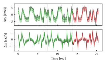
Figure 3: Error prediction (mean $\pm$ one standard deviation) from the learned residual model with $\bm{\phi}_{\mathrm{Taylor}}$ 7 on training (green) and testing (red) data for lateral velocity (top) and yaw rate (bottom), respectively.

TABLE I: State prediction errors for different learning models

Prediction error		No model learning	Gaussian Process	BLR with $\bm{\phi}_{\text{Taylor}}$
$v_{y}$ [cm/s]	train	$3.81\pm 0.21$	$\mathbf{0.82\pm 0.04}$	$1.66\pm 0.09$
	test	$3.85\pm 0.26$	$\mathbf{1.07\pm 0.14}$	$1.77\pm 0.05$
$\omega$ [rad/s]	train	$0.46\pm 0.03$	$0.21\pm 0.02$	$\mathbf{0.18\pm 0.02}$
	test	$0.44\pm 0.02$	$0.22\pm 0.01$	$\mathbf{0.18\pm 0.01}$

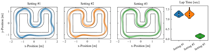
Figure 4: Three plots on the left: Density of the car’s position across 20 laps for three different settings. Setting #1: Nominal model and sub-optimal controller weights. Setting #2: Residual dynamics learning and same controller weights as previous setting. Setting #3: Residual dynamics learning with tuned controller weights. Right plot: corresponding lap times for the three settings.

Although the linear model in 6 that is used to learn the residual dynamics has only two parameters per dimension, it is able to approximate the residual dynamics to high accuracy. Fig. 3 shows the predicted error (solid line) and the corresponding uncertainty estimates (shaded region) for the lateral velocity (top) and yaw rate (bottom), respectively. The training data corresponds to two complete laps around the track (predicted values in green) and the testing data to one lap (predicted values in red). Qualitatively, the model is capable of predicting the true error signal (gray) without overfitting. For a more quantitative analysis, we compare our model with a GP in terms of the RMSE in Table I. Uncertainty estimates for the prediction error correspond to the standard deviation from 50 models trained on independently sampled training (2 laps) and testing data (1 lap). We note that learning with either model helps to drastically improve the predictive capabilities over the nominal dynamics model. Notably, BLR with $\bm{\phi}_{\text{Taylor}}$ even outperforms the GP for the yaw rate indicating that our model strikes a good balance between complexity and expressiveness.

V-C Joint Optimization: Key to High-Performance Racing

Next, we want to demonstrate the importance of both model learning as well as controller tuning for high-performance racing. To this end, we drive 20 laps with three different settings and record the respective lap times: Setting #1 serves as the benchmark, for which the controller weights are not tuned and we solely use the nominal model $f(\mathbf{x},\mathbf{u})$ in the MPCC. From Fig. 4 we can see that the car reliably makes it around the track albeit resulting in a clearly sub-optimal trajectory. Especially after turns with high velocity (bottom left and right), the car repeatedly bumped into the track’s boundaries. For setting #2, we use the same controller weights, but account for errors in the dynamics by learning a residual model $g(\mathbf{x},\mathbf{u})$. The car’s trajectory is slightly improved and does not bounce against the boundaries anymore. Interestingly, while model learning leads to a change in the car’s trajectory, it does not directly translate to a reduction of the lap time as depicted on the right in Fig. 4. In setting #3, we changed the controller weights such that the driving behaviour is more aggressive. Consequently, the car’s trajectory is greatly improved and the lap time is reduced by well over a second. Note that the combination of aggressive controller weights without model learning repeatedly lead to the car crashing into the track’s boundary from which it could not recover. We conclude that both accurate dynamics as well as a well-tuned controller are required for high-performance racing, justifying the joint optimization approach.

V-D Optimal Controllers Depend on Context

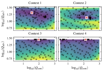
Figure 5: Response surfaces of the regularized objective function 8 for different contexts. We vary the contouring cost $Q_{\mathrm{cont}}$ as well as the advancing parameter $Q_{\mathrm{adv}}$ from the MPCC formulation 4. Note that the overall shape of the response surfaces are similar across all contexts, i.e., a decrease in $Q_{\mathrm{adv}}$ leads to an increase in the objective. However, the locations of the estimated optima, i.e., minimum of the GP posterior mean function (red cross), are different for the contexts. Note that we had to decrease the parameter space for car 2 (contexts 3 and 4) in order to avoid that the car either crashes into the track boundary (too high $Q_{\mathrm{adv}}$) or did not make sufficient progress and regularly stopped (too low $Q_{\mathrm{adv}}$).

The main hypothesis of this paper is that the MPCC’s parameters require adaptation under different environmental conditions. In order to confirm this hypothesis, the goal of the next experiment is to approximately find the response surface of the following objective for different contexts

$$J(\bm{\theta})=T_{\mathrm{lap}}+\lambda\cdot\bar{\Delta}_{\mathrm{centerline}}$$ (8)

with $T_{\mathrm{lap}}$ denoting the lap time, $\bar{\Delta}_{\mathrm{centerline}}$ is the average distance of the car to the centerline in centimeters and $\lambda$ is a parameter governing the trade-off between the two cost terms. The regularizing term penalizes too aggressive behaviour of the controller resulting in the car crashing due to cutting the track’s corners. To emulate the different driving conditions, we use two different cars each with and without an additional mass of 40 grams (corresponding to about 30% of the cars’ total weight) attached to the chassis, leading to a total of four different contexts. Note that the additional mass influences the inertia, traction and steering behaviour of the cars. For each context, we record 200 laps, where after every second lap we change the controller’s weights and evaluate the objective on the lap thereafter, thus accounting for transient effects due to the change of the weights. For the first 70 iterations, the controller weights are sampled from a low-discrepancy sequence to sufficiently explore the full parameter space and the remaining 30 parameter vectors are chosen according to the UCB acquisition function to exploit the objective around the vicinity of the estimated optimum. We show the respective GP mean estimates of the objective function as well as its minimum (red cross) in Fig. 5. The response surfaces vary considerable across the contexts and so do the optimal controller weights. However, there are also some common features, e.g., a low advancing parameter $Q_{\text{adv}}$ in 4 generally leads to a cautious driving behaviour and therefore an increased lap time.

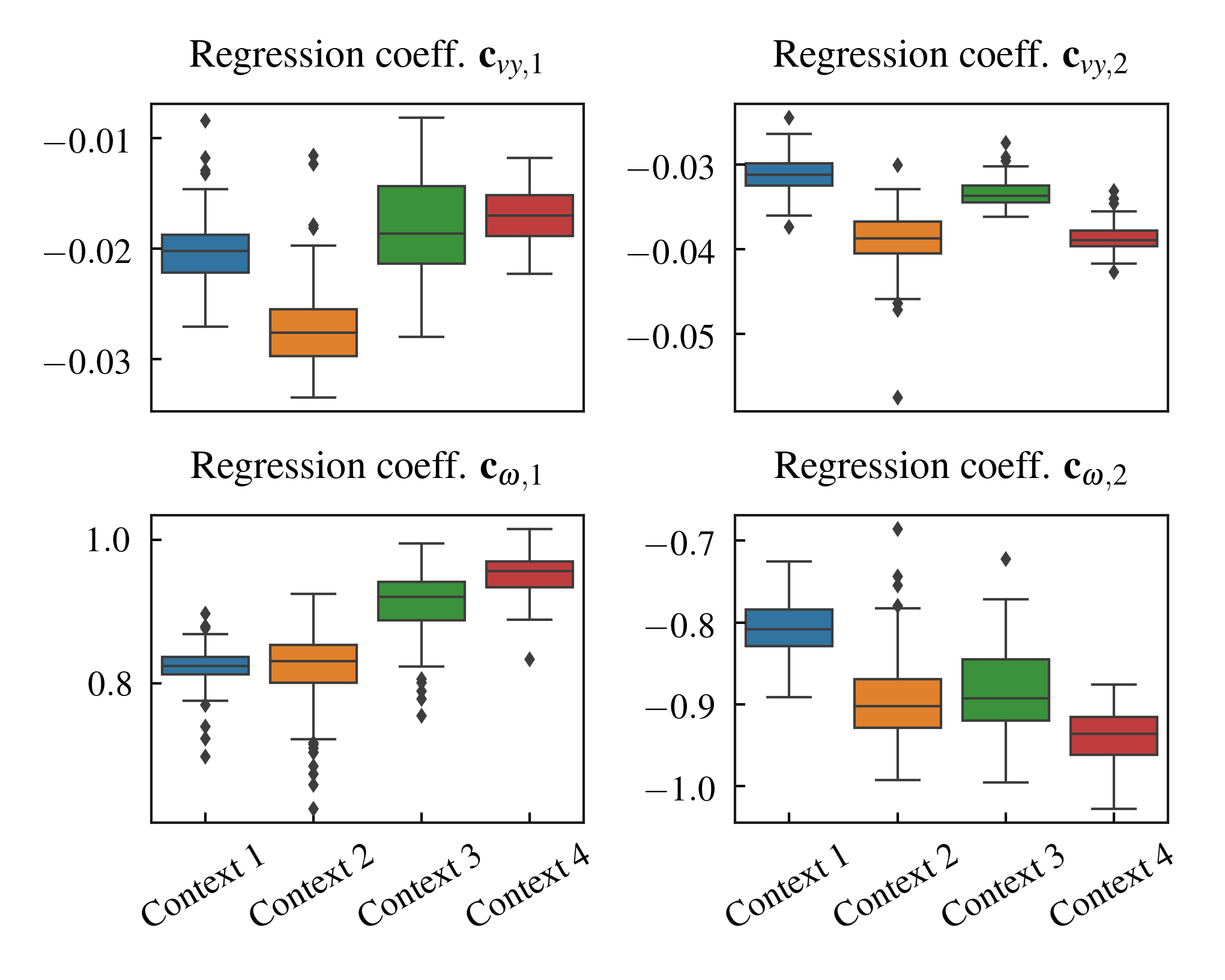
Figure 6: Distributions of the regression coefficients $\mathbf{c}_{vy}$ and $\mathbf{c}_{\omega}$ from 6 for four different contexts. The regression coefficients are re-estimated every lap and the data was obtained from the same experiment depicted in Fig. 5. In total, each sample distribution is based on 140 laps per context.

The goal of this paper is to utilize the knowledge collected from previous experiments to accelerate the search for optimal controller parameters in new contexts. As such, the residual model must be able to encode different environmental conditions via the regression coefficients $\mathbf{C}$ in 6 as context and adapt accordingly if the conditions change. To this end, we re-estimate the regression coefficients after every lap based on the telemetry data from the previous lap. Due to the ever changing data, we expect the regression coefficients to fluctuate slightly, even for the same context. We therefore investigate if a change in the car’s true dynamics leads to distinguishably different context variables despite the stochasticity mentioned above. Based on the data from the previous experiment (200 laps per context), we show the respective distributions of the four regression coefficients in Fig. 6. While the respective distributions exhibit outliers, the different contexts lead to regression coefficients that are clearly distinguishable from each other and as such can serve as suitable descriptors for the respective changes in the dynamics. We hypothesize that the outliers originate from situations where the cars shortly loose traction and start to drift, which is not well captured by either the nominal or residual linear model based on the custom features.

V-E Contextual Controller Tuning

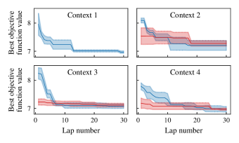
Figure 7: Learning progress of standard BO (blue), i.e., without using contextual information, compared to contextual BO (red). The figure shows mean $\pm$ standard deviation as solid line and shaded region, respectively. Utilizing the contextual information from different cars significantly improves the initial phase of the controller tuning problem.

In the final experiment, we show that utilizing the contextual information from previous runs accelerates the search for the optimal controller parameters. We again consider the four different contexts from the previous experiments. For each context, we first use standard BO to minimize the regularized lap time 8 by adapting the weights $Q_{\text{adv}}$ and $Q_{\text{cont}}$ in the MPCC formulation. The results for standard BO (blue) are shown in Fig. 7, where the solid lines represent the mean across three independent experiments and the shaded region corresponds to the standard deviation. For each context, we see that BO reliably finds the controller weights that lead to the objective’s minimum. However, note that each time the optimization is started from scratch such that the initial lap times are relatively high because the algorithm has to explore the full parameter space. For contextual BO (red), we now utilize the collected data from the other experiments to pre-train the objective’s surrogate GP model. In particular, we accumulate the collected data in order, meaning that for context 2 the GP is initialized with the 30 iterations from context 1. For the last context, we utilize all 90 data points from the previous three contexts. The results clearly show that by transferring the knowledge between the contexts, the optimization is accelerated drastically and even the first iterate already leads to a good behaviour.

VI Conclusion

We have presented a framework to combine model learning and controller tuning with application to high-performance autonomous racing. In particular, we proposed to encode the environmental condition via a residual dynamics model such that knowledge between different contexts can be shared to reduce the effort for controller tuning. The benefits of the proposed approach have been demonstrated on a custom hardware platform with an extensive experimental evaluation. Key for the method’s success was the low-dimensional representation of the environment by means of the custom parametric model. For more complex learning models such as neural networks, one could for example obtain a low-dimensional context via (variational) auto-encoders, which we leave for future research.

References

- [1] L. Hewing, K. P. Wabersich, M. Menner, and M. N. Zeilinger, “Learning-based model predictive control: Toward safe learning in control,” Annu. Rev. Control Robot. Auton. Syst., vol. 3, pp. 269–296, 2020.
- [2] C. D. McKinnon and A. P. Schoellig, “Learn fast, forget slow: Safe predictive learning control for systems with unknown and changing dynamics performing repetitive tasks,” IEEE Robot. Autom. Lett., vol. 4, no. 2, pp. 2180–2187, 2019.
- [3] J. G. Ziegler and N. B. Nichols, “Optimum settings for automatic controllers,” J. Dyn. Syst. Meas. and Control, vol. 115, 1942.
- [4] N. Hansen and A. Ostermeier, “Completely derandomized self-adaptation in evolution strategies,” Evolutionary computation, vol. 9, no. 2, pp. 159–195, 2001.
- [5] D. R. Jones, C. D. Perttunen, and B. E. Stuckman, “Lipschitzian optimization without the lipschitz constant,” J. Optim. Theory and Appl., vol. 79, no. 1, pp. 157–181, 1993.
- [6] P. I. Frazier, “A tutorial on Bayesian optimization,” arXiv:1807.02811, 2018.
- [7] K. Chatzilygeroudis, V. Vassiliades, F. Stulp, S. Calinon, and J.-B. Mouret, “A survey on policy search algorithms for learning robot controllers in a handful of trials,” IEEE Trans. Robot., 2019.
- [8] I. Bogunovic, J. Scarlett, and V. Cevher, “Time-varying gaussian process bandit optimization,” in Proc. Int. Conf. on Artif. Intell. and Stat. (AISTATS), 2016.
- [9] M. Tesch, J. Schneider, and H. Choset, “Adapting control policies for expensive systems to changing environments,” in Proc. IEEE/RSJ Int. Conf. Intell. Robots and Syst. (IROS), 2011.
- [10] L. P. Fröhlich, E. D. Klenske, J. Vinogradska, C. G. Daniel, and M. N. Zeilinger, “Noisy-input entropy search for efficient robust Bayesian optimization,” in Proc. Int. Conf. on Artif. Intell. and Stat. (AISTATS), 2020.
- [11] M. Quigley, B. Gerkey, K. Conley, J. Faust, T. Foote, J. Leibs, E. Berger, R. Wheeler, and A. Ng, “ROS: an open-source robot operating system,” in Proc. IEEE Intl. Conf. on Robot. and Autom. (ICRA) Workshop on Open Source Robot., 2009.
- [12] A. Wilson, A. Fern, and P. Tadepalli, “Using trajectory data to improve Bayesian optimization for reinforcement learning,” J. Mach. Learn. Res., vol. 15, no. 1, pp. 253–282, 2014.
- [13] S. Bansal, R. Calandra, T. Xiao, S. Levine, and C. J. Tomlin, “Goal-driven dynamics learning via Bayesian optimization,” in Proc. IEEE Conf. Dec. and Control, 2017.
- [14] M. Gevers, “Identification for control: From the early achievements to the revival of experiment design,” Europ. J. Control, vol. 11, no. 4, pp. 335–352, 2005.
- [15] L. P. Fröhlich, E. D. Klenske, C. G. Daniel, and M. N. Zeilinger, “High-dimensional Bayesian optimization for policy search via automatic domain selection,” in Proc. IEEE/RSJ Int. Conf. Intell. Robots and Syst. (IROS), 2019.
- [16] M. O’Kelly, H. Zheng, A. Jain, J. Auckley, K. Luong, and R. Mangharam, “Tunercar: A superoptimization toolchain for autonomous racing,” in Proc. IEEE Int. Conf. Robot. Autom. (ICRA), 2020.
- [17] W. Edwards, G. Tang, G. Mamakoukas, T. Murphey, and K. Hauser, “Automatic tuning for data-driven model predictive control,” in Proc. IEEE Int. Conf. Robot. Autom. (ICRA), 2021.
- [18] A. Krause and C. S. Ong, “Contextual gaussian process bandit optimization.” in Adv. Neural Inform. Proces. Syst. (NeurIPS), 2011.
- [19] E. V. Bonilla, K. M. A. Chai, and C. K. I. Williams, “Multi-task gaussian process prediction,” in Adv. Neural Inform. Proces. Syst. (NeurIPS), 2008.
- [20] J. H. Metzen, A. Fabisch, and J. Hansen, “Bayesian optimization for contextual policy search,” in Proc. 2nd Mach. Learning Planning Control Robot Motion Workshop, 2015.
- [21] B. Yang, G. Wang, R. Calandra, D. Contreras, S. Levine, and K. Pister, “Learning flexible and reusable locomotion primitives for a microrobot,” IEEE Robot. Autom. Lett., vol. 3, no. 3, pp. 1904–1911, 2018.
- [22] T. Seyde, J. Carius, R. Grandia, F. Farshidian, and M. Hutter, “Locomotion planning through a hybrid bayesian trajectory optimization,” in Proc. IEEE Int. Conf. Robot. Autom. (ICRA), 2019.
- [23] M. Fiducioso, S. Curi, B. Schumacher, M. Gwerder, and A. Krause, “Safe contextual bayesian optimization for sustainable room temperature PID control tuning,” in Proc. Int. Joint Conf. Artif. Intell. (IJCAI), 2019.
- [24] F. Berkenkamp, A. P. Schoellig, and A. Krause, “Safe controller optimization for quadrotors with Gaussian processes,” in Proc. IEEE Int. Conf. Robot. Autom. (ICRA), 2016.
- [25] A. Fabisch and J. H. Metzen, “Active contextual policy search,” J. Mach. Learn. Res., vol. 15, no. 1, pp. 3371–3399, 2014.
- [26] D. Metz and D. Williams, “Near time-optimal control of racing vehicles,” Automatica, vol. 25, no. 6, pp. 841–857, 1989.
- [27] D. Lam, C. Manzie, and M. Good, “Model predictive contouring control,” in Proc. IEEE Conf. Dec. and Control, 2010.
- [28] R. Verschueren, S. De Bruyne, M. Zanon, J. V. Frasch, and M. Diehl, “Towards time-optimal race car driving using nonlinear mpc in real-time,” in Proc. IEEE Conf. Dec. and Control, 2014.
- [29] A. Liniger, A. Domahidi, and M. Morari, “Optimization-based autonomous racing of 1: 43 scale rc cars,” Optim. Control Applicat. Methods, vol. 36, no. 5, pp. 628–647, 2015.
- [30] L. Hewing, J. Kabzan, and M. N. Zeilinger, “Cautious model predictive control using gaussian process regression,” IEEE Trans. Control Syst. Techn., vol. 28, no. 6, pp. 2736–2743, 2019.
- [31] J. Kabzan, L. Hewing, A. Liniger, and M. N. Zeilinger, “Learning-based model predictive control for autonomous racing,” IEEE Robot. Autom. Lett., vol. 4, no. 4, pp. 3363–3370, 2019.
- [32] U. Rosolia and F. Borrelli, “Learning how to autonomously race a car: A predictive control approach,” IEEE Trans. Control Syst. Techn., vol. 28, no. 6, pp. 2713–2719, 2020.
- [33] A. Wischnewski, J. Betz, and B. Lohmann, “A model-free algorithm to safely approach the handling limit of an autonomous racecar,” in Proc. IEEE Int. Conf. Conn. Veh. Expo (ICCVE), 2019.
- [34] A. Jain and M. Morari, “Computing the racing line using bayesian optimization,” in Proc. IEEE Conf. Dec. and Control, 2020.
- [35] C. D. McKinnon and A. P. Schoellig, “Context-aware cost shaping to reduce the impact of model error in receding horizon control,” in Proc. IEEE Int. Conf. Robot. Autom. (ICRA), 2020.
- [36] R. Rajamani, Vehicle Dynamics and Control, ser. Mechanical Engineering Series. Springer Science & Business Media, 2011.
- [37] H. Pacejka, Tyre and Vehicle Dynamics, ser. Automotive Engineering Series. Elsevier, 2002.
- [38] A. Domahidi and J. Jerez, “Forces professional,” embotech GmbH (http://embotech. com/FORCES-Pro), 2014.
- [39] A. Zanelli, A. Domahidi, J. Jerez, and M. Morari, “FORCES NLP: an efficient implementation of interior-point methods for multistage nonlinear nonconvex programs,” Int. J. Control, vol. 93, no. 1, pp. 13–29, 2017.
- [40] C. E. Rasmussen and C. K. I. Williams, Gaussian Processes for Machine Learning. MIT Press, 2006.
- [41] C. M. Bishop, Pattern Recognition and Machine Learning. Springer, 2006.