Dispersion properties of plasmonic sub-wavelength elliptical wires wrapped with graphene

Abstract

One fundamental motivation to know the dispersive, or frequency dependent characteristics of localized surface plasmos (LSPs) supported by elliptical shaped particles wrapped with graphene sheet, as well as their scattering characteristics when these elliptical LSPs are excited, is related with the design of plasmonic structures capable to manipulate light at sub-wavelength scale. The anisotropy imposed by the ellipse eccentricity can be used as a geometrical tool for controlling plasmonic resonances. Unlike metallic case, where the multipolar eigenmodes are independent of each others, we find that the induced current on graphene boundary couples multipolar eigenmodes with the same parity. In the long wavelength limit, a recursive relation equation for LSPs in term of the ellipse eccentricity parameter is derived and explicit solutions at lowest order are presented. In this approximation, we obtain analytical expressions for both the anisotropic polarizability tensor elements and the scattered power when LSPs are excited by plane wave incidence.

1 Introduction

Light scattering properties on metallic wire particles with non-circular cross section have been extensively studied [1, 2]. The two-dimensional geometrical anisotropy leads to a splitting in two or more plasmon branches corresponding to the lowest energy states, instead of one as occur in the circular case, which are evidenced on the angular optical response of the wire [3]. This fact together with other outstanding properties have found applications in some optical topics requiring field hot spots, such as surface enhanced Raman and optical nano-antennas development [4, 5, 6, 7].

Sub-wavelength structures coated with a graphene sheet provide a suitable alternative to metallic elements because they exhibit relative low loss and highly tunable, via electrostatic gating or chemical doping [8], surface plasmons in the frequency region from microwaves to infrared [9]. The small plasmon wavelength, which usually reaches values smaller than one tenth of the wavelength of the photon of the same frequency, deals with the possibility to build smaller plasmonic constituent elements, a feature positioning the graphene as a promising platform to the development of controllable plasmon devices, in particular of a new generation of sensors and modulators from microwaves to the mid-infrared regimes [10, 11, 12, 13] constituting an intersection between optics and electronic.

Graphene layers structures has attracted wide attention in many applications due to a strong adsorption capacity for contaminants [14, 15], electrical properties [16, 17, 18] and improved light harvesting [19, 20, 21].

In the framework of electromagnetic scattering by sub-wavelength graphene particles, an extensive wealth of theoretical analysis have been developed, allowing possible a wide range of applications based on the interaction between graphene and electromagnetic radiation via LSP mechanisms, including sensing [22, 23], superscattering [24, 25], low energy spasers [26, 27, 28, 30], PT-symmetric structures tailoring lasing modes [29, 30], and micro and nano antennas [31, 32, 33, 34].

This work deals with the plasmon properties of an elliptical dielectric wire wrapped with graphene. The LSP branches corresponding to lower eigenmodes are obtained by solving the homogeneous problem, i.e., the scattering problem without external excitation. Unlike the metallic case, where LSP eigenmodes are uncoupled between them, the current density on graphene coating couples all multipolar LSPs with the same parity given rise to an infinite set of coupled equations for the field amplitude. Moreover, the tangential direction of charge oscillation on graphene covered leads to a counterintuitive splitting: the low dipolar frequency mode corresponds to polarizability oscillations along minor ellipse axis while the high dipolar frequency mode corresponds to polarizability oscillations along the major ellipse axis. In this framework, analytical expressions of the anysotropic polarizability is found. We also provided analytical expressions for the scattered power when the graphene elliptical wire is excited by a plane wave. All scattering curves are compared with those obtained by applying a rigorous formalism based in the Green surface integral method [35, 36] valid for arbitrary shaped cross sections.

This paper is organized as follows. Firstly, in Section 2 we develop an analytical method based on the separation of variables in elliptical coordinates and obtain an approximated solution for the electromagnetic field scattered by an elliptical wire cover with graphene. This approach allows us to express each of the amplitudes in the multipolar expansion of the fields as a series of power of the ellipse eccentricity. In Section 3 we present the results related with the dispersive characteristics and the scattering calculations for a dielectric wire wrapped with graphene. Finally, concluding remarks are provided in Section 4. The Gaussian system of units is used and an $\mbox{exp}(-i\omega t)$ time-dependence is implicit throughout the paper, with $\omega$ as the angular frequency, $t$ as the time, and $i=\sqrt{-1}$. The symbols Re and Im are respectively used for denoting the real and imaginary parts of a complex quantity.

2 Theory

2.1 Scattered field equations

We consider an elliptical dielectric cylinder wrapped with graphene sheet. The elliptical profile has the major semi-axis $a$ along $x$ axis and the minor semi-axis $b$ along the $y$ axis. We use elliptical coordinates, which are related with the Cartesian coordinates by following relations

$$\begin{array}[]{ll}x=l\cosh(\rho)\cos(\phi),\\ y=l\sinh{}(\rho)\sin(\phi),\\ z=z\end{array}$$ (1)

$\rho$ and $\phi$ are the radial and angular elliptical coordinates. The unit vectors $\hat{\rho}$ and $\hat{\phi}$ are normal and tangent along elliptical shape, respectively (see Figure 1). In this way, the boundary curve of the ellipse is given by $\rho=\rho_{0}$, $\tanh(\rho_{0})=b/a$, with the major semi-axis $a=l\cosh(\rho_{0})$ along the $x$ axis and the minor semi-axis $b=l\sinh(\rho_{0})$ along the $y$ axis. The scale parameter $l$ is related with $a$ and $b$ by the following $l=\sqrt{a^{2}-b^{2}}$.

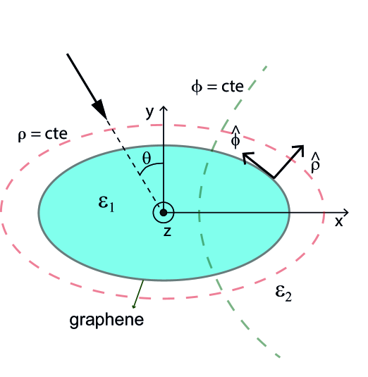
Figure 1: Schematic illustration of the elliptical wire wrapped with graphene. The wire ($\varepsilon_{1}$ and surface conductivity $\sigma$) is embedded in a transparent medium with permittivity $\varepsilon_{2}$. Both media are non magnetic, $\mu_{1}=\mu_{2}=1$.

The magnetic field inside the elliptic cylinder $\rho<\rho_{0}$ can be expressed as follows:

$$H^{(1)}(\rho,\phi)=\sum_{m=1}^{+\infty}a_{m}\sinh(m\rho)\sin(m\phi)+c_{m}\cosh(m\rho)\cos(m\phi),$$ (2)

and the field outside the ellipse $\rho>\rho_{0}$ is expressed as,

$$H^{(2)}(\rho,\phi)=\sum_{m=1}^{+\infty}b_{m}e^{-m\rho}\sin(m\phi)+d_{m}e^{-m\rho}\cos(m\phi)+H^{(inc)}.$$ (3)

where the last term corresponds to the incident magnetic field. Firstly, we suppose a plane wave incidence with the electric field along the $x$ axis and amplitude $E_{0}$. In this case, the incident magnetic field in the long wavelength limit is written as

$$H^{(inc)}(\rho,\phi)=-ik_{0}E_{0}\varepsilon_{2}l\sinh(\rho)\sin(\phi).$$ (4)

The symmetry imposed by the incident field direction imposes the amplitudes $c_{m}$ and $d_{m}$ in the field expressions (2) and (3) to be zero. By using the Ampere-Maxwell equation, we can relate the components of the electric field and the $z$-component of the magnetic field as follows,

$$\mathbf{E}^{(j)}=-\frac{1}{ik_{0}\varepsilon_{j}}\mathbf{\nabla}_{t}\times\hat{z}H^{(j)}$$ (5)

$j=1,\,2$,

$$\mathbf{\nabla}_{t}=\frac{1}{f(\rho_{0},\phi)}\left[\hat{\rho}\frac{\partial}{\partial\rho}+\hat{\phi}\frac{\partial}{\partial\phi}\right]$$ (6)

is the transverse part of the $\mathbf{\nabla}$ operator and $f(\rho_{0},\phi)=l\sqrt{\cosh^{2}(\rho)-\cos^{2}(\phi)}$. The boundary condition along the contour of the ellipse $\rho=\rho_{0}$ is written as [37],

$$\begin{array}[]{ll}\frac{1}{\varepsilon_{1}}\frac{\partial H^{(1)}}{\partial\rho}|_{\rho_{0}}=\frac{1}{\varepsilon_{2}}\frac{\partial H^{(2)}}{\partial\rho}|_{\rho_{0}}\\ \left[H^{(2)}+H^{(inc)}-H^{(1)}\right]|_{\rho_{0}}=\frac{4\pi\sigma}{c}[E^{(2)}_{\phi}+E^{(inc)}_{\phi}]|_{\rho_{0}}.\end{array}$$ (7)

Using field expressions (2) and (3) with $c_{m}=d_{m}=0$ into the boundary condition (7) and projecting into the Fourier basis, two system of equations for amplitudes $a_{m}$ and $b_{m}$ are obtained. Then, we can eliminate amplitudes $a_{m}$ to obtain one set of equations for amplitudes $B_{m}=b_{m}e^{-m\rho_{0}}$ (see appendix B),

$$B_{k}t_{k}+\sum_{m\not=k}^{+\infty}M_{km}B_{m}=Q_{k},$$ (8)

with

$$M_{km}=\frac{4\pi\sigma}{ck_{0}\varepsilon_{2}}ims_{km},$$ (9)

$$t_{k}=1+\frac{\varepsilon_{1}}{\varepsilon_{2}}\tanh(k\rho_{0})+M_{kk},$$ (10)

$$Q_{k}=ik_{0}E_{0}(\varepsilon_{2}-\varepsilon_{1})l\sinh(\rho_{0})\delta_{k1}+\frac{4\pi\sigma}{c}E_{0}\coth(\rho_{0})s_{k1}.$$ (11)

2.2 Lowest order eccentricity

Before studying the scattering problem given by Eq. (8), we first study the homogeneous problem (or eigenmodes problem), i.e., the scattering problem without an external source ($E_{0}=0$ in Eq. (8)). To do this, we consider the homogeneous part in Eq. (8) which can be rewritten as

$$B_{k}t_{k}+\sum_{m\not=k}^{+\infty}M_{km}B_{m}=0,$$ (12)

Since in the limit of null eccentricity $\tanh(k\rho_{0})=1$ for $\rho=\infty$, the first term in Eq. (12) reduces to the dispersion relation of a cylinder with circular cross section for the $k$ multipolar order, while the second term reduce to zero. For small values of eccentricity, $e=l/b=\sqrt{(a/b)^{2}-1}<<1$, we can expand Eq. (12) in powers of $e$ as follows. Taking into account that the matrix element is of order $O(2)$ for $k\not=m$ (see appendix C), $s_{km}\approx e^{2}$, from Eq. (9) we deduce that $M_{1m}$ is at last of order $O(2)$ and thus we can expand the homogeneous equation (12) in powers of $e$. The form that Eq. (12) takes for $k=1$ is,

$$B_{1}t_{1}+\sum_{m\not=1}^{+\infty}M_{1m}B_{m}=0,$$ (13)

and the form that Eq. (12) takes for $m\not=1$ is,

$$B_{m}=-\frac{M_{m1}}{t_{m}}B_{1}-\sum_{n\not=1,m}^{+\infty}\frac{M_{mn}}{t_{m}}B_{n}.$$ (14)

Replacing Eq. (14) into Eq. (13), we obtain

$$B_{1}t_{1}-\sum_{m\not=1}^{+\infty}M_{1m}\frac{M_{m1}}{t_{m}}B_{1}-\sum_{m\not=1}^{+\infty}\sum_{n\not=1,m}^{+\infty}M_{1m}\frac{M_{mn}}{t_{m}}B_{n}=0.$$ (15)

Following the same steps as described above, we solve Eq. (12) by iteration,

$$t_{1}-\sum_{m\not=1}^{+\infty}M_{1m}\frac{M_{m1}}{t_{m}}-\sum_{m\not=1}^{+\infty}\sum_{n\not=1,m}^{+\infty}M_{1m}\frac{M_{mn}}{t_{m}}\frac{M_{n1}}{t_{n}}+...=0.$$ (16)

This equation is the dispersion relation of elliptical LSPs on graphene. To find the LSP characteristics, we consider the lowest order, $e^{4}$, in the dispersion relation (16),

$$t_{1}-M_{13}\frac{M_{31}}{t_{3}}=0,$$ (17)

which can be made explicit using Eqs. (9) and (10) as follows

$$\left(1+\frac{\varepsilon_{1}}{\varepsilon_{2}}\tanh(\rho_{0})+\frac{4\pi\sigma}{ck_{0}\varepsilon_{2}}is_{11}\right)$$

$$\times\left(1+\frac{\varepsilon_{1}}{\varepsilon_{2}}\tanh(3\rho_{0})+3\frac{4\pi\sigma}{ck_{0}\varepsilon_{2}}is_{33}\right)+3\left(\frac{4\pi\sigma}{ck_{0}\varepsilon_{2}}\right)^{2}(s_{13})^{2}=0,$$ (18)

where we have used $s_{13}=s_{31}$ and the fact that $s_{12}=s_{21}=0$. The expressions for $s_{1m}$ and $s_{33}$ until order $e^{2}$ can be obtained from Eq. (C) (see appendix C),

$$s_{11}=\frac{1}{b}\left[1-\frac{3}{8}e^{2}\right],$$

$$s_{13}=\frac{1}{b}\frac{1}{8}e^{2},$$

$$s_{33}=\frac{1}{b}\left[1-\frac{1}{4}e^{2}\right].$$ (19)

We note that for null eccentricity, the matrix element $s_{13}=0$ and $\tanh(\rho_{0})=\tanh(3\rho_{0})=1$, as a consequence the dispersion relation (2.2) reduces to a product between two factors, both corresponding to a circular cylinder. One of these factors corresponds to the dispersion relation of the dipolar order ($m=1$) and the other corresponds to the hexapolar order ($m=3$). For small values of eccentricity, the matrix element $s_{13}\not=0$ and consequently the last term in Eq. (2.2) is not null, with which Eq. (2.2) represents the elliptical LSP dispersion relation. Note that the coupling mechanism between the dipolar and the hexapolar orders is evidenced by the presence of the last term in the dispersion equation (2.2).

It is worth nothing that Eq. (2.2) is the lowest order of the elliptical LSP dispersion relation. This is true because the truncation of Eq. (15) at order $O(4)$ in eccentricity admit only modes $m\leq 4$. In addition, for higher orders, $O(2N)$ for example, Eq. (15) couples $m=1,\,3,\,5,...,2N-1$ multipolar orders.

At the same order in eccentricity as we have written Eq. (17), from Eq. (8) we can obtain the dipolar coefficient $b_{1}$ for the scattering of a plane wave (non homogeneous problem) polarized along $x$ axis,

$$b_{1}=E_{0}e^{\rho_{0}}\widetilde{b_{1}},$$ (20)

where

$$\widetilde{b_{1}}=\frac{A_{x}}{t_{1}t_{3}-M_{13}M_{31}},$$ (21)

and

$$A_{x}=\left(ik_{0}b[\varepsilon_{2}-\varepsilon_{1}]+\frac{4\pi\sigma s_{11}}{c\tanh(\rho_{0})}\right)$$

$$\times\left(1+\frac{\varepsilon_{1}}{\varepsilon_{2}}\tanh(3\rho_{0})+\frac{4\pi\sigma i3s_{33}}{ck_{0}\varepsilon_{2}l\sinh(\rho_{0})}\right)$$

$$-\left(\frac{4\pi\sigma}{c}\right)^{2}\frac{\cosh(\rho_{0})is_{13}s_{31}}{k_{0}\varepsilon_{2}l\sinh^{2}(\rho_{0})}$$ (22)

Once the scattering amplitude $b_{1}$ is found, the polarizability $\alpha_{x}$ is given by (see appendix D)

$$\alpha_{x}=\frac{i(a+b)}{4k_{0}}\widetilde{b_{1}}.$$ (23)

Following the same steps that allow us to obtain Eq. (17) but taking the electric field along the $y$ axis, we obtain the lowest order dispersion equation for $y$ polarization,

$$\left(1+\frac{\varepsilon_{1}}{\varepsilon_{2}}\coth(\rho_{0})+\frac{4\pi\sigma}{ck_{0}\varepsilon_{2}}iv_{11}\right)\left(1+\frac{\varepsilon_{1}}{\varepsilon_{2}}\coth(3\rho_{0})+3\frac{4\pi\sigma}{ck_{0}\varepsilon_{2}}iv_{33}\right)$$

$$+3\left(\frac{4\pi\sigma}{ck_{0}\varepsilon_{2}}\right)^{2}(v_{13})^{2}=0,$$ (24)

$$v_{11}=\frac{1}{a}\left[1+\frac{3}{8}e^{2}\right],$$

$$v_{13}=v_{31}=\frac{1}{a}\frac{1}{8}e^{2},$$

$$v_{33}=\frac{1}{a}\left[1+\frac{1}{4}e^{2}\right].$$ (25)

At the same order in eccentricity as we have written Eq. (2.2), the dipolar coefficient $d_{1}$ for the scattering of a plane wave polarized along $y$ axis,

$$d_{1}=E_{0}e^{\rho_{0}}\widetilde{d_{1}},$$ (26)

where $d_{1}$ is the dipolar amplitude of the scattered field in medium 2 for $y$ polarization and

$$\widetilde{d_{1}}=\frac{A_{y}}{q_{1}q_{3}-N_{13}N_{31}},$$ (27)

where

$$A_{y}=\left(ik_{0}b[\varepsilon_{2}-\varepsilon_{1}]+\frac{4\pi\sigma v_{11}}{c\coth(\rho_{0})}\right)$$

$$\times\left(1+\frac{\varepsilon_{1}}{\varepsilon_{2}}\coth(3\rho_{0})+\frac{4\pi\sigma i3v_{33}}{ck_{0}\varepsilon_{2}l\cosh(\rho_{0})}\right)$$ (28)

$$-\left(\frac{4\pi\sigma}{c}\right)^{2}\frac{\sinh(\rho_{0})iv_{13}v_{31}}{k_{0}\varepsilon_{2}l\cosh^{2}(\rho_{0})},$$ (29)

and

$$q_{k}=1+\frac{\varepsilon_{1}}{\varepsilon_{2}}\coth(k\rho_{0})+N_{kk},$$ (30)

$$N_{mk}=\frac{4\pi\sigma}{ck_{0}\varepsilon_{2}}imv_{km}.$$ (31)

The corresponding polarizability $\alpha_{y}$ is given by (see appendix D)

$$\alpha_{y}=\frac{i(a+b)}{4k_{0}}\widetilde{d_{1}}.$$ (32)

It is interesting to note that in the limit of $\rho_{0}\rightarrow\infty$, the polarizabilities (23) and (32) tend to the value corresponding to the circular case,

$$\alpha_{c}=\varepsilon_{2}\frac{b^{2}}{2}\left[\frac{\varepsilon_{1}-\varepsilon_{2}+\frac{4\pi\sigma i}{ck_{0}b}}{\varepsilon_{1}+\varepsilon_{2}+\frac{4\pi\sigma i}{ck_{0}b}}\right].$$ (33)

Polarizabilities (23) and (32) constitutes the central object for optical interactions where the quasistatic regime is applicable [38], such as enhanced and confined optical near–fields [39], metasurface and metagrating applications [40] and nanoparticles bonding [41, 42, 43]. In the present work, we use these expressions to calculate the power scattered by the particle in the quasistatic limit as follows. Taking into account that the radiated power by a point dipole $\mathbf{p}$ is [44],

$$P=\frac{\pi\omega^{3}}{4c^{2}}|\mathbf{p}|^{2},$$ (34)

and neglecting third order contributions, we can replace the induced dipole moment components $p_{j}=\alpha_{j}\,E_{0}$ ($j=x,\,y$) to calculate the power scattered by the elliptical particle in the dipolar limit. Considering that the incident power is $P_{0}=\frac{c}{8\pi}E_{0}^{2}2L_{i}$, $L_{i}=a,\,b$ for $x$ and $y$ polarization, respectively, the normalized power scattered by the particles is written as

$$\frac{P_{i}}{P_{0}}=\frac{\pi^{2}\omega^{3}}{L_{i}c^{3}}|\alpha_{i}|^{2}.$$ (35)

3 Results

In this section we use the formalism developed in the above section to calculate the eigenfrequencies and the scattering cross section curves. In all the examples the wire is immersed in vacuum ($\varepsilon_{2}=\mu_{2}=1$), the dielectric core has a permittivity $\varepsilon_{1}=3.9$ and permeability $\mu_{1}=1$. The graphene parameters are $T=300$K and $\gamma_{g}=0.1$ meV.

In order to explore the effects that the departure from the circular geometry has on the dispersive characteristics of LSPs, we compare the results obtained for all elliptical shapes with those obtained in the circular case with the same perimeter. We assume that the perimeter is sufficiently large to describe the optical properties of the wires as characterized by the same local surface conductivity as planar graphene (see appendix A). Moreover, since the aroused interest on graphene due to plasmonic properties in THz and IR frequency regions, graphene–coated wires with a micro-sized cross section have become an attractive platform for optical applications (see [45, 46, 47] and Refs. therein). In this way, we have chosen a perimeter equal to $\pi\,\mu$m for all examples, excepting those presented in Fig. 5a where we have selected $\pi/2\,\mbox{and}\,\pi/4\,\mu$m. Even though nonlocal effects could appear in our system for frequencies lower than characteristic resonance frequencies, this is not interesting for our purposes (see appendix E).

Firstly, we evaluate the coupling mechanism between multipolar orders provided by the graphene current. To do this, by solving Eq. (8) we calculate the amplitude modulus $|b_{m}|$ for $m=1$ and $3$ (both non-null lowest order) as a function of $\omega/c$ frequency and for three values of eccentricity, $a/b=1.05,\,1.2$ and $1.4$. Without loss of generality we made the calculation for horizontal (or $x$) polarization (electric field parallel to $x$ axis). For the lowest eccentricity value of $a/b=1.05$ we observe that the amplitude $b_{1}$ reaches it maximum value ($\approx 10$) at $\hbar\omega=31.52$meV corresponding to the dipolar excitation. At the same frequency, the amplitude $b_{3}$ reaches a local maximum ($\approx 0.1$), evidencing the coupling between third and first order modes. This means that the amplitude $b_{3}$ not only contributes to the scattered field at the resonance frequency of the $m=1$ order (where the $|b_{1}|$ amplitude reaches the absolute maximum value), a fact that also occur on metallic nanoparticles [1, 48, 49, 50] for which the field amplitudes are decoupled, but also reaches a local maximum at this frequency.

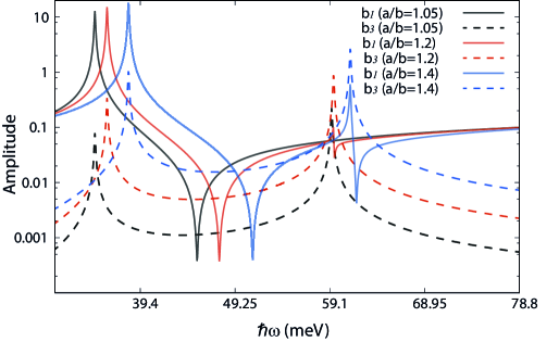
Figure 2: Amplitudes $b_{m}$ modulus ($m=1$ and $3$) as a function of $\omega/c$ frequency for $a/b=1.05,\,1.2,\,1.4$ and for $x$ polarization. The perimeter of the ellipse is $\pi\,\mu$m and chemical potential $\mu_{g}=0.5eV$.

On the other hand, the amplitude $b_{3}$ reaches the absolute maximum value at $\hbar\omega\approx 59$meV corresponding to the hexapolar order excitation, while the first order amplitude $b_{1}$ shows a local maximum and minimum at this frequency value. As eccentricity values are increasing, two effects are observed: on the one hand, dipolar and hexapolar order frequencies moves to higher values and, on the other hand, the coupling mechanism between different orders appear more visible, as can be seen in Figure 2 where the local maximum value of $b_{3}$ curve at the resonant dipolar frequency (where the $b_{1}$ amplitude reaches the absolute maximum value) increases with the value of $a/b$. The same behavior is observed near $\hbar\omega\approx 59$meV, where the local variation of the $b_{1}$ amplitude at the hexapolar resonant frequency is more visible with the $a/b$ increment. These results show how a non–zero surface conductivity on graphene couples different orders of the same parity (see second term in Eq. (8)) causing all these modes to reach a local maximum at the resonant frequency of one of them.

In the vertical (or $y$) polarization (electric field parallel to $y$ axis) case (not shown in Figure 2), we obtain similar results with the only exception that the resonant frequency is a decreasing function of the eccentricity $a/b$, instead of being increasing as occur in the $x$ polarization case.

In order to gain insight about the resonant frequency dependence with the eccentricity of the wire, we solve the homogeneous problem at lowest order in eccentricity to obtain the dispersion equation for lower modes. Figure 3 shows the dispersion relation as a function of $a/b$ ($a/b\leq 1.4$) and the scattering curves for both horizontal and vertical polarization for $a/b=1.2$ ($e=0.66$). From Figure 3a we see two branches, the upper branch, calculated with Eq. (17), corresponds to $x$ polarization and the lower branch, calculated with Eq. (2.2), corresponds to $y$ polarization. For null eccentricity, $a=b$, these two branches converge to the value $\hbar\omega=34.28$meV corresponding to the case of circular cross section. As the value of eccentricity increases, the gap between two branches increases leading to an increment in the splitting between resonance frequencies when the structure is illuminated with a plane wave. In Figure 3b we plotted the scattering curves for plane wave incidence by using Eq. (35) with $i=x$ and $i=y$ for $x$ and $y$ polarization, respectively, (continuous line). The calculation also was made by using a rigorous method based on the Green surface integral method (GSIM) (dashed line) [35]. Two peaks are observed. The lower frequency peak, angle of incidence $\theta=90^{\circ}$, corresponds to excitation of $y$-polarized LSPs, i.e., surface plasmons whose polarizability $\alpha_{y}$ is along the $y$ axis. The upper frequency peak, angle of incidence $\theta=0$, correspond to excitation of $x$-polarized LSPs, i.e., surface plasmons whose polarizability $\alpha_{x}$ is along the $x$ axis. Both resonance frequencies agree well with the values calculated from the dispersion equation. We also observe a small red shifting of the resonance peaks calculated using GSIM with respect to those calculated using Eq. (35).

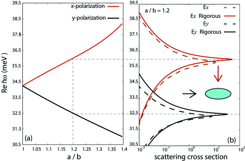
Figure 3: (a) Real part of the eigenfrequencies as a function of $\frac{a}{b}$ ($\frac{a}{b}=\sqrt{e^{2}+1}$). (b) Scattering cross section for incidence direction parallel to $y$ axis (electric field along $x$ axis) and parallel to y axis (electric field along the $y$ axis). Continuous lines correspond to the calculus using Eq. (35) and dashed line curves correspond to calculation using GSIM. The arrows indicate the incident direction. The perimeter of the ellipse is $\pi\,\mu$m and chemical potential $\mu_{g}=0.5$eV.

It is worth noting that unlike metallic structures, where the lower modal frequency is associated to oscillations along the major axis (the $x$ axis in the present case) and the upper modal frequency is along the minor axis (the $y$ axis in the present case), from Figure 3 we see that the situation is completely other way around for graphene wrapped wires. This fact is due to the geometrical difference between the charge oscillations on each of the systems. While in the metallic case the displacement of charge is along the induced electric field, in the graphene particles case, the movement of charge is along the boundary elliptical curvature.

In order to study the behavior with graphene parameters, we calculate the eigenfrequency dependence on chemical potential. Figure 4 shows the eigenfrequency branches, one for $x$ polarization and the other for $y$ polarization, for various values of the chemical potential, $\mu_{g}=0.6,\,0.7,\,0.8,\,0.9,\,1$eV. We observe that eigenfrequencies of the upper and lower branches increase with the chemical potential increment. This is consistent with the fact that frequency plasmonic resonances for circular cross section cylinders are proportional to $\sqrt{\mu_{g}}$ [52].

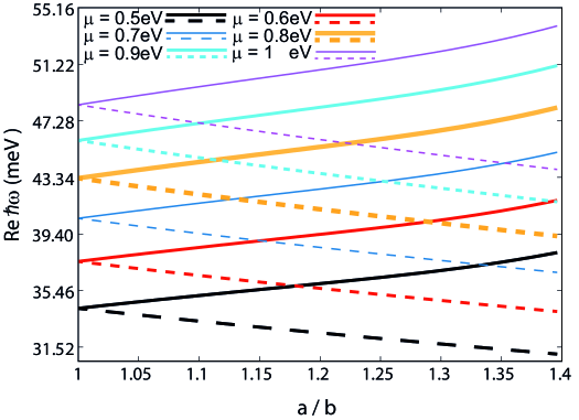
Figure 4: Real part of the eigenfrequencies as a function of $\frac{a}{b}$ ($\frac{a}{b}=\sqrt{e^{2}+1}$) for $\mu_{g}=0.6,\,0.7,\,0.8,\,0.9,\,1$eV. Solid lines correspond to $x$ polarization and dashed lines corresponds to $y$ polarization. Other parameters are the same as in Figure 3

Finally, we calculate the dependence of the eigenfrequencies with the size and the contrast between external and internal constitutive parameters. In Figure 5a we observe that both branches, corresponding to $x$ and $y$ polarizations, increase their frequencies as the ellipse perimeter is decreased from $\pi$ to $\pi/4\,\mu$m. This fact can be understood from the circular case studied in [52], where we have demonstrated that the eigenfrequency depends on the radius as $\omega\approx R^{-1/2}$. In Figure 5b we have plotted the eigenfrequency branches for three values of the permittivity of the internal medium, $\varepsilon_{1}=3.9,\,3,\,2.13$. We observe that Re$\,\hbar\omega$ increases with the decreasing of the permittivity value. This behavior is consistent with the fact that the eigenfrequency depends on permittivities as $\omega\approx(1+\varepsilon_{1})^{-1/2}$ for circular graphene wires [52].

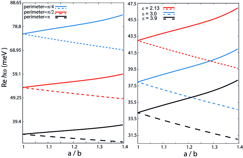
Figure 5: Real part of the eigenfrequencies as a function of $\frac{a}{b}$ ($\frac{a}{b}=\sqrt{e^{2}+1}$). (a) $\varepsilon_{1}=3.9$ and various values of perimeters: $\pi,\,\pi/2,\,\pi/4\,\mu$m, (b) for perimeter equal to $\pi\mu$m and various values of permittivities, $\varepsilon_{1}=3.9,\,3,\,2.13$. The chemical potential is $\mu_{g}=0.5$eV. Solid lines correspond to $x$ polarization and dashed lines corresponds to $y$ polarization.

4 Conclusion

In conclusion, we have analytically studied the dispersive characteristics for an ellipical dielectric wire wrapped with graphene. We have found two branches corresponding to the lowest frequency band, one of them corresponds to eigenmodes with a dipole moment along the major axis and the other with a dipole moment along the minor axis of the wire elliptical cross section. Interestingly, we found that contrary to what happens in the metallic plasmonic case, the low dipolar frequency branch corresponds to polarizability oscillations along minor ellipse axis and the high dipolar frequency eigenmode corresponds to polarizability oscillations along the major ellipse axis. We have found analytical expressions for the polarizability elements along the ellipse axis which reduces to that of the circular shaped wire as the eccentricity parameter tends to zero.

We think that the results provided in this work can be employed for a deeper interpretation of the dispersive characteristics of elliptical graphene plasmons, which opens up possibilities for practical applications using structures capable to manipulate light at sub-wavelength scale.

Appendix A Graphene conductivity

The graphene layer is considered as an infinitesimally thin layer with a frequency-dependent surface conductivity $\sigma(\omega)$ given by the Kubo formula [51], $\sigma=\sigma^{intra}+\sigma^{inter}$, with the intraband and interband contributions given by

$$\sigma^{intra}(\omega)=\frac{2ie^{2}k_{B}T}{\pi\hbar^{2}(\omega+i\gamma_{g})}\mbox{ln}\left[2\mbox{cosh}(\mu_{g}/2k_{B}T)\right],$$ (A1)

$$\sigma^{inter}(\omega)=\frac{e^{2}}{\hbar}\Bigg{\{}\frac{1}{2}+\frac{1}{\pi}\mbox{arctan}\left[(\hbar\omega-2\mu_{g})/2k_{B}T\right]-$$

$$\frac{i}{2\pi}\mbox{ln}\left[\frac{(\hbar\omega+2\mu_{g})^{2}}{(\hbar\omega-2\mu_{g})^{2}+(2k_{B}T)^{2}}\right]\Bigg{\}},$$ (A2)

where $\mu_{g}$ is the chemical potential (controlled with the help of a gate voltage), $\gamma_{g}$ the carriers scattering rate, $e$ the electron charge, $k_{B}$ the Boltzmann constant and $\hbar$ the reduced Planck constant.

Appendix B Boundary conditions

By replacing Eqs. (2) and (3) into Eq. (7) we obtain a set of two coupled equations for amplitudes $a_{m}$ and $b_{m}$,

$$\sum_{m=1}^{+\infty}\left(\frac{a_{m}}{\varepsilon_{1}}\cosh(m\rho_{0})m+m\frac{b_{m}}{\varepsilon_{2}}e^{-m\rho_{0}}\right)\sin(\phi)=\frac{1}{\varepsilon_{2}}\frac{\partial H^{(inc)}}{\partial\rho}$$ (B1)

$$\sum_{m=1}^{+\infty}\left(b_{m}e^{-m\rho_{0}}-a_{m}\sinh(m\rho_{0})+\frac{4\pi\sigma}{ck_{0}\varepsilon_{2}}imb_{m}e^{-m\rho_{0}}\frac{1}{f(\rho_{0},\phi)}\right)$$

$$\times\sin(m\phi)=$$

$$-H^{(inc)}|_{\rho_{0}}+\frac{4\pi\sigma}{ck_{0}\varepsilon_{2}}i\frac{1}{f(\rho_{0},\phi)}\frac{\partial H^{(inc)}}{\partial\rho}|_{\rho_{0}}.$$ (B2)

Note that the left hand side of Eq. (B1) is written as a sine Fourier series, then we can expand the right hand side as a sine series and find, performing Fourier integral, a lineal equation between amplitudes $a_{m}$ and $b_{m}$,

$$\frac{a_{k}}{\varepsilon_{1}}\cosh(k\rho_{0})k+\frac{b_{k}}{\varepsilon_{2}}ke^{-k\rho_{0}}=-ik_{0}E_{0}l\cosh(\rho_{0})\delta_{k1}.$$ (B3)

Contrary, Eq. (B) presents a difficulty related with the graphene current factor $f^{-1}(\rho_{0},\phi)$. Multiplying Eq. (3) by $\sin(k\phi)$ ($k\geq 1$) and integrating in $[-\pi,\,\pi]$, we obtain,

$$b_{k}e^{-k\rho_{0}}-a_{k}\sinh(k\rho_{0})+\sum_{m=1}^{+\infty}\frac{4\pi\sigma}{ck_{0}\varepsilon_{2}}imb_{m}e^{-m\rho_{0}}s_{km}=$$

$$-h_{k}+\frac{4\pi\sigma}{ck_{0}\varepsilon_{2}}idh_{k},$$ (B4)

where

$$s_{km}=\frac{1}{\pi}\int_{-\pi}^{\pi}\frac{1}{f(\rho_{0},\phi)}\sin(m\phi)\sin(k\phi)d\phi$$ (B5)

$$h_{k}=\frac{1}{\pi}\int_{-\pi}^{\pi}H^{(inc)}|_{\rho}\sin(k\phi)d\phi$$ (B6)

$$dh_{k}=\frac{1}{\pi}\int_{-\pi}^{\pi}\frac{1}{f(\rho_{0},\phi)}\frac{\partial H^{(inc)}}{\partial\rho}|_{\rho_{0}}\sin(k\phi)d\phi.$$ (B7)

Note that both functions $H^{(inc)}|_{\rho_{0}}$ and $\frac{\partial H^{(inc)}}{\partial\rho}|_{\rho_{0}}$ have an angular dependence $\approx\sin(\phi)$ and thus $h_{k}\approx\delta_{k1}$ and $dh_{k}\approx s_{km}\delta_{m1}$. Therefore, Eq. (B) can be written as,

$$b_{k}e^{-k\rho_{0}}-a_{k}\sinh(k\rho_{0})+\sum_{m=1}^{+\infty}\frac{4\pi\sigma}{ck_{0}\varepsilon_{2}}imb_{m}e^{-m\rho_{0}}s_{km}=$$

$$ik_{0}E_{0}\varepsilon_{2}l\sinh(\rho_{0})\delta_{k1}+\frac{4\pi\sigma}{c}E_{0}\coth(\rho_{0})s_{k1}.$$ (B8)

Note that in absence of graphene, i.e. $\sigma=0$, the system of Eqs. (B3) and (B) are uncoupled for field amplitudes. Contrary, in presence of graphene, the graphene current term in the left hand side of Eq. (B) couples orders with the same parity. This is true because the matrix elements $s_{km}\not=0$ provided that $m+k$ be even (Eq. (B5)).

By eliminatig the amplitudes $a_{m}$ from Eqs. (B3) and (B), we obtain an equation for amplitudes $b_{m}$,

$$b_{k}e^{-k\rho_{0}}\left(1+\frac{\varepsilon_{1}}{\varepsilon_{2}}\tanh(k\rho_{0})+\frac{4\pi\sigma}{ck_{0}\varepsilon_{2}}iks_{kk}b_{k}e^{-k\rho_{0}}\right)+$$

$$\sum_{m\not=k}^{+\infty}\frac{4\pi\sigma}{ck_{0}\varepsilon_{2}}imb_{m}e^{-m\rho_{0}}s_{km}=$$

$$ik_{0}E_{0}(\varepsilon_{2}-\varepsilon_{1})l\sinh(\rho_{0})\delta_{k1}+\frac{4\pi\sigma}{c}E_{0}\coth(\rho_{0})s_{k1}.$$ (B9)

Appendix C Explicit form of $s_{km}$ matrix elements

We expand the current factor as power of $\sin(\phi)$,

$$\frac{1}{h(\rho_{0},\phi)}=\frac{1}{\sinh(\rho_{0})\sqrt{1+\sin^{2}(\phi)e^{2}}}=$$

$$\frac{1}{\sinh(\rho_{0})}[1-\sin^{2}(\phi)\frac{1}{2}e^{2}+\frac{3}{8}\sin^{4}(\phi)e^{4}-\frac{5}{16}\sin^{6}(\phi)e^{6}$$

$$+\frac{35}{128}\sin^{8}(\phi)e^{8}-\frac{63}{226}\sin^{10}(\phi)e^{10}$$

$$+\frac{231}{1024}\sin^{12}(\phi)e^{12}-\frac{429}{2048}\sin^{14}(\phi)e^{14}+...].$$ (C1)

Note that the expansion (C) is valid for $a/b<\sqrt{2}$. By replacing Eq. (C) into Eq. (B5), we obtain

$$s_{km}=\frac{1}{b\pi}\int_{-\pi}^{\pi}[1-\sin^{2}(\phi)\frac{1}{2}e^{2}+\frac{3}{8}\sin^{4}(\phi)e^{4}$$

$$-\frac{5}{16}\sin^{6}(\phi)e^{6}+\frac{35}{128}\sin^{8}(\phi)e^{8}-\frac{63}{226}\sin^{10}(\phi)e^{10}$$

$$+\frac{231}{1024}\sin^{12}(\phi)e^{12}-\frac{429}{2048}\sin^{14}(\phi)e^{14}+...]$$

$$\times\sin(m\phi)\sin(k\phi)d\phi.$$ (C2)

From this equation, we can see that $s_{km}\approx e^{2}$ ($s_{km}$ is of order $O(2)$) for $k\not=m$. For example, if we consider $k=1$, it is straightforward verify,

$$s_{1m}=\frac{1}{b}[\delta_{m1}-\frac{e^{2}}{2}\left(\frac{3}{4}\delta_{m1}-\frac{1}{4}\delta_{m3}\right)$$

$$+\frac{3}{8}e^{4}\left(\frac{5}{8}\delta_{m1}-\frac{5}{16}\delta_{m3}+\frac{11}{16}\delta_{m5}\right)+...].$$ (C3)

We can see that $s_{11}$ is of order $O(0)$, $s_{13}$ is of order $O(2)$, $s_{15}$ is order $O(4)$, …, $s_{1m}$ is order $O(m-1)$.

Appendix D Field of a dipole moment placed at the origin

We consider a line dipole source (whose axis lies along the $z$ axis) with a dipole moment $\mathbf{p}$ is placed at the origin. The magnetic field is along the $z$ axis ($\mathbf{H}(\mathbf{r})=\phi(\mathbf{r})\hat{r}$). The wave equation for $\phi(\mathbf{r})$ when the retardation is negligible reads

$$\nabla^{2}\phi(\mathbf{r})=-4\pi ik_{0}\mathbf{p}\times\nabla\delta(\mathbf{r}).$$ (D1)

The solution $\phi(\mathbf{r})$ of Eq. (D1) can be written as

$$\phi(\mathbf{r})=ik_{0}\mathbf{p}\times\nabla f(\mathbf{r}),$$ (D2)

where $f(\mathbf{r})$ satisfies

$$\nabla^{2}\phi(\mathbf{r})=-4\pi\delta(\mathbf{r}).$$ (D3)

By solving Eq. (D3) we obtain $\phi(\mathbf{r})=-2\log(\mathbf{r})$. Then, the magnetic field $\phi(\mathbf{r})$ of a point dipole calculated using Eq. (D2) in elliptical coordinates (1) is given by

$$\phi(\mathbf{r})=-2ik_{0}\frac{p_{x}\sinh{\rho}\sin\phi-p_{y}\cosh{\rho}\cos\phi}{l(\cosh^{2}{\rho}-\sin^{2}{\phi})},$$ (D4)

where $p_{x}$ and $p_{y}$ are the Cartesian components of the dipole moment $\mathbf{p}$. For $\rho$ values large enough, this expression can be rewritten as

$$\phi(\mathbf{r})=-4ik_{0}\frac{p_{x}\sin\phi-p_{y}\cos\phi}{l}e^{-\rho}.$$ (D5)

By comparing this equation (with $p_{y}=0$) with the first term in the scattered field given in Eq. (3) we obtain the induced electrical dipole as a function of the $b_{1}$ scattering amplitude

$$p_{x}=\frac{il}{4k_{0}}b_{1}=\frac{il}{4k_{0}}E_{0}e^{\rho_{0}}\widetilde{b_{1}}=\frac{i(a+b)}{4k_{0}}E_{0}\widetilde{b_{1}},$$ (D6)

where the sub-index stand for the direction of the dipole moment. In the last equality in Eq. (D6) we have used $le^{\rho_{0}}=a+b$. Finally, dividing Eq. (D6) by $E_{0}$, the corresponding polarizability $\alpha_{x}$ is obtained.

In the similar way, by comparing Eq. (D5) (with $p_{x}=0$) with the second term in Eq. (3) we obtain the induced electrical dipole

$$p_{y}=\frac{il}{4k_{0}}d_{1}=\frac{il}{4k_{0}}E_{0}e^{\rho_{0}}\widetilde{d_{1}}=\frac{i(a+b)}{4k_{0}}E_{0}\widetilde{d_{1}}.$$ (D7)

By dividing Eq. (D7) by the incident field amplitude $E_{0}$, we obtain the $\alpha_{y}$ polarizability (32).

Appendix E Nonlocal response in graphene conductivity

The objective of this section is to provide information about the relation between the local graphene conductivity response considered in this work and the dimensions of the proposed structure. The local approximation begins to break down as a reduction of the structure takes place. The nonlocality or spatial dispersion in graphene conductivity arises when the plasmon phase velocity $v_{SP}$ is slow and comparable with the electron Fermi velocity $v_{F}\approx 10^{12}\,\mu m/s$. Since, we focused on cylindrical structures whose cross section is a slight deviation from the circular cross section, an estimation of their size can be made by considering a cylinder with circular cross section and radius $R$ ($a<R<b$). Taking into account the small size of the cylinder, $R/\lambda<<1$ ( $\lambda=2\pi/\omega$ the wavelength), the phase velocity of plasmons $v_{SP}=k_{SP}/\omega$ can be estimated by using the quasistatic approximation. In this way, the surface plasmon effective momentum $k_{SP}$, which is along the azimutal angle ($\phi$ axis), can be written as [52],

$$k_{SP}=\frac{m}{R},$$ (E1)

where $m$ is the eigenmode order. If we consider $m=1$ (dipolar order), the factor

$$\frac{v_{F}}{v_{SP}}=\frac{v_{F}}{R\,\omega}\approx\frac{10^{12}\mu\mbox{m}/s}{R\,\frac{\omega}{c}\,3\times 10^{14}\mu m/s}=\frac{1}{R\,\frac{\omega}{c}\,300}.$$ (E2)

The smaller $\frac{v_{F}}{v_{SP}}$ in Eq. (E2), the better the local conductivity approximation. For example, if we consider a value $\frac{v_{F}}{v_{SP}}<1/10$, graphene local conductivity differs less than 1$\%$ from that considering non local effects [38]. As a consequence, our method is acceptable provided that

$$R\,\frac{\omega}{c}>\frac{1}{30}.$$ (E3)

Equation (E3) establishes a reasonable limit for the applicability of our model. Figure 6 shows a map with two regions. In one of them the nonlocal effects can be neglected (upper region), whereas in the other (lower region) these effects become important. The curve separating these regions corresponds to $R$ values, named $R_{c}$, for which the equality in Eq. (E3) is fulfilled.

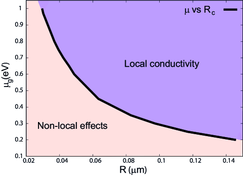
Figure 6: Regions of the plane $\mbox{R}-\mu_{g}$ (radius and chemical potential) where, according to Eq. (E3), local and non local effects take place. The curve separating these two regions corresponds to critical values of the radius, $R_{c}$, that verify the equality in Eq. (E3) for varying $\mu_{g}$ values.

References

- [1] C. F. Bohren and D. R. Huffman, Absorption and scattering of light by small particles (New York: Wiley, 1983).
- [2] S. A. Maier, Plasmonics: Fundamentals and Applications, (Springer, New York, 2007)
- [3] Klimov, V. Nanoplasmonics, (PanStanford Publishing: Singapore, 2012).
- [4] O.J.F. Martin, Plasmon Resonances in Nanowires with a Non-regular Cross-Section, In: Tominaga J., Tsai D.P. (eds) Optical Nanotechnologies. Topics in Applied Physics, vol 88. Springer, Berlin, Heidelberg.
- [5] Kneipp, K., Moskovits, M., Kneipp, H., eds. (2006) Surface-Enhanced Raman Scattering (Springer, Berlin).
- [6] Kuhn S, Hakanson U, Rogobete L, Sandoghdar V, Enhancement of single-molecule fluorescence using a gold nanoparticle as an optical nanoantenna. Phys. Rev. Lett., (2006) 97, 017402.
- [7] Faggiani R, Yang J and Lalanne P, ACS Photonics 2, (2015) 1739-1744
- [8] Xia F . NatPhotonics 7, (2013) 420
- [9] Jablan J , Soljacic M , Buljan H . Proc IEEE 101, 1689-704 (2013)
- [10] E. Piccinini, S. Alberti, G. S. Longo, T. Berninger, J. Breu, J. Dostalek, O. Azzaroni, and W. Knoll, Pushing the Boundaries of Interfacial Sensitivity in Graphene FET Sensors: Polyelectrolyte Multilayers Strongly Increase the Debye Screening Length, J. Phys. Chem. C 122, (2018) 10181-10188
- [11] D Stefanatos, V Karanikolas, N Iliopoulos, E Paspalakis, Fast spin initialization of a quantum dot in the Voigt configuration coupled to a graphene layer, Physica E: Low-dimensional Systems and Nanostructures 117, (2020) 113810
- [12] D Cano, A Ferrier, K Soundarapandian, A Reserbat-Plantey, M Scarafagio, A Tallaire, A Seyeux, P Marcus, H de Riedmatten, P Goldner, F H. L. Koppens, and K J Tielrooij, Fast electrical modulation of strong near-field interactions between erbium emitters and graphene, Nat Commun 11, 4094 (2020)
- [13] Raad, S.H., Atlasbaf, Z. and Zapata-RodrÃguez, C.J. Broadband absorption using all-graphene grating-coupled nanoparticles on a reflector. Sci Rep 10, 19060 (2020).
- [14] R. Chen, Y. Cheng, P. Wang, Q. Wang, S. Wan, S. Huang, R. Su, Y. Song, Y. Wang, Enhanced removal of Co(II) and Ni(II) from high-salinity aqueous solution using reductive self-assembly of three–dimensional magnetic fungal hyphal/graphene oxide nanofibers, Science of The Total Environment 756, (2021), 143871.
- [15] M. Zhang, L. Zhang, S. Tian, X. Zhang, J. Guo, X. Guan, P. Xu, Effects of graphite particles/Fe3 on the properties of anoxic activated sludge, Chemosphere 253 (2020) 126638.
- [16] M. Zhang, X. Song, X. Ou, Y. Tang, Rechargeable batteries based on anion intercalation graphite cathodes, Energy Storage Materials 16, (2019) 65–84
- [17] H. Yin, C. Han, Q. Liu, F. Wu, F. Zhang, Y. Tang, Recent Advances and Perspectives on the Polymer Electrolytes for Sodium/Potassium–Ion Batteries, Small 17, (2021) 2006627.
- [18] X. Zhang ,Y. Tang ,F. Zhang and C. Lee, A Novel Aluminum–Graphite Dual-Ion Battery, Adv. Energy Mater 6, ( 2016) 1502588.
- [19] X. Miao, S. Tongay, M. K. Petterson, K. Berke, A. G. Rinzler, B. R. Appleton, and A. F. Hebard, High Efficiency Graphene Solar Cells by Chemical Doping, Nano Lett. 12, (2012) 2745-2750.
- [20] X. Du, J. Li, G. Niu, J. Yuan, K. Xue, M. Xia, W. Pan, X. Yang, B. Zhu, and J. Tang, Lead halide perovskite for efficient optoacoustic conversion and application toward high-resolution ultrasound imaging, Nat. Commun. 12, (2021) 3348
- [21] Z. Ni, X. Cao, X. Wang, S. Zhou, C. Zhang, B. Xu, and Y. Ni , Facile Synthesis of Copper(I) Oxide Nanochains and the Photo-Thermal Conversion Performance of Its Nanofluids, Coatings 11, (2021) 749
- [22] E. A. Velichko, Evaluation of a graphene-covered dielectric microtube as a refractive-index sensor in the terahertz range, J. Opt. 18, 035008 (2016).
- [23] H Farmani, A Farmani, Z Biglari, A label-free graphene-based nanosensor using surface plasmon resonance for biomaterials detection, Physica E: Low-dimensional Systems and Nanostructures 116, 113730 (2020)
- [24] SH Raad, CJ Zapata-RodrÃguez, Z Atlasbaf, Graphene-coated resonators with frequency-selective super-scattering and super-cloaking, Journal of Physics D: Applied Physics 52 (49), 495101
- [25] M Gingins, M Cuevas, and R A Depine, Surface plasmon dispersion engineering for optimizing scattering, emission, and radiation properties on a graphene spherical device, Applied Optics 59, (2020) 4254-4262
- [26] O. L. Berman, R. Y. Kezerashvili, and Y. E. Lozovik, Graphene nanoribbon based spaser, PHYSICAL REVIEW B 88, 235424 (2013)
- [27] S. B. Ardakani and R. Faez, Tunable spherical graphene surface plasmon amplification by stimulated emission of radiation, Journal of Nanophotonics 13, 026009 (2019).
- [28] L Prelat, M Cuevas, N Passarelli, RB Marún, R Depine, Spaser and optical amplification conditions in graphene-coated active wires, Journal of the Optical Society of America B 38, 2118–2126 (2021)
- [29] W Zhang, T Wu, and X Zhang, Tailoring Eigenmodes at Spectral Singularities in Graphene-based PT Systems, Scientific Reports 7, (2017) 11407
- [30] M Cuevas, MK Habil, CJ Zapata-Rodríguez, Lasing condition for trapped modes in subwavelength-wired PT-symmetric resonators, Optics Express 29, (2021) 10192-10208
- [31] J. M. Jornet and I. F. Akyildiz, Graphene-based Plasmonic Nano-Antenna for Terahertz Band Communication in Nanonetworks,” in IEEE Journal on Selected Areas in Communications, vol. 31, no. 12, pp. 685-694
- [32] D. Correas-Serrano, J. S. Gomez-Diaz, A. Alu, and A. Alvarez-Melcon, Electrically and magnetically biased graphene-based cylindrical waveguides: Analysis and applications as reconfigurable antennas, IEEE Trans. Terahertz Sci. Technol. 5, 951 (2015)
- [33] M Cuevas, Theoretical investigation of the spontaneous emission on graphene plasmonic antenna in THz regime, Superlattices and Microstructures 122, (2020) 216-227
- [34] Z Ullah,G Witjaksono, I Nawi, N Tansu, M I Khattak, and M Junaid, A Review on the Development of Tunable Graphene Nanoantennas for Terahertz Optoelectronic and Plasmonic Applications, Sensors 20, ( 2020) 1401.
- [35] C Valencia, M A Riso, M Cuevas, R A Depine, J. Opt. Soc. Am. B 34, (2017) 1075-1083
- [36] M Cuevas, Spontaneous emission in plasmonic graphene subwavelength wires of arbitrary sections, Journal of Quantitative Spectroscopy and Radiative Transfer 206, (2018) 157-162
- [37] Riso M, Cuevas M and Depine R A, Tunable plasmonic enhancement of light scattering and absorption in graphenecoated subwavelength wires, Journal of Optics 17, (2015) 075001
- [38] Christensen, T., Jauho, A., Wubs, M. and Mortensen, N. A., Localized plasmons in graphene-coated nanospheres, Phys. Rev. B 91, (2015) 125414.
- [39] S. Bidault, M. Mivelle, and N. Bonod, Dielectric nanoantennas to manipulate solid-state light emission, J. Appl. Phys. 126, 094104 (2019).
- [40] D. R. Abujetas, J. Olmos-Trigo, J. J. Sáenz, and J. A. Sánchez-Gil, Coupled electric and magnetic dipole formulation for planar arrays of particles: Resonances and bound states in the continuum for all-dielectric metasurfaces, Phys. Rev. B 102, (2020) 125411.
- [41] PC Chaumet,and M Nieto-Vesperinas, “Optical binding of particles with or without the presence of a flat dielectric surface,” Phys. Rev. B 64, 035422 (2001).
- [42] N Kostina, M Petrov, A Ivinskaya, S Sukhov, A Bogdanov, I Toftul, M Nieto-Vesperinas, P Ginzburg, and A Shalin, “Optical binding via surface plasmon polariton interference,” Phys. Rev. B 99, 125416 (2019).
- [43] NA Kostina, DA Kislov, AN Ivinskaya, A Proskurin, DN Redka, A Novitsky, P Ginzburg, and AS Shalin, “Nanoscale Tunable Optical Binding Mediated by Hyperbolic Metamaterials,” ACS Photonics 7, (2020), 425–433.
- [44] M Cuevas, Graphene coated subwavelength wires: a theoretical investigation of emission and radiation properties, Journal of Quantitative Spectroscopy and Radiative Transfer 200, (2017) 190-197
- [45] R A Depine Graphene Optics: Electromagnetic solution of canonical problems (IOP Concise Physics. San Raefel, CA, USA: Morgan and Claypool Publishers 2017)
- [46] D Teng, K Wang, Z Li, Graphene-coated nanowire waveguides and their applications, Nanomaterials 10, (2020) 229
- [47] D. O. Herasymova, S. Dukhopelnykov, A. Nosich, Infrared diffraction radiation from twin circular dielectric rods covered with graphene: plasmon resonances and beam position sensing, J Opt. Soc.of Am. B 38, (2021)
- [48] H. Mertens, A. F. Koenderink, and A. Polman, “Plasmon-enhanced luminescence near noble-metal nanospheres: Comparison of exact theory and an improved Gersten and Nitzan model,” Phys. Rev. B 76, 115123 (2007).
- [49] V. Karanikolas, C. A. Marocico, and A. L. Bradley, Spontaneous emission and energy transfer rates near a coated metallic cylinder, Phys. Rev. A 89, 063817 (2014)
- [50] J. Barthes, A. Bouhelier, A. Dereux and G Colas des Francs, Coupling of a dipolar emitter into one-dimensional surface plasmon, Sci. Rep. 3, 2734 (2013)
- [51] Falkovsky FA, Optical properties of graphene and IV-VI semiconductors, Phys. Usp. 51 887-897
- [52] M. Cuevas, M. A. Riso, and R. A. Depine, Complex frequencies and field distributions of localized surface plasmon modes in graphene-coated subwavelength wires, J. Quant. Spectrosc. Radiat. Transfer 173, 26-33 (2016).