Parameterised population models of transient non-Gaussian noise in the LIGO gravitational-wave detectors

Abstract

The two interferometric LIGO gravitational-wave observatories provide the most sensitive data to date to study the gravitational-wave Universe. As part of a global network, they have just completed their third observing run in which they observed many tens of signals from merging compact binary systems. It has long been known that a limiting factor in identifying transient gravitational-wave signals is the presence of transient non-Gaussian noise, which reduce the ability of astrophysical searches to detect signals confidently. Significant efforts are taken to identify and mitigate this noise at the source, but its presence persists, leading to the need for software solutions. Taking a set of transient noise artefacts categorised by the GravitySpy software during the O3a observing era, we produce parameterised population models of the noise projected into the space of astrophysical model parameters of merging binary systems. We compare the inferred population properties of transient noise artefacts with observed astrophysical systems from the GWTC2.1 catalogue. We find that while the population of astrophysical systems tend to have near equal masses and moderate spins, transient noise artefacts are typically characterised by extreme mass ratios and large spins. This work provides a new method to calculate the consistency of an observed candidate with a given class of noise artefacts. This approach could be used in assessing the consistency of candidates found by astrophysical searches (i.e. determining if they are consistent with a known glitch class). Furthermore, the approach could be incorporated into astrophysical searches directly, potentially improving the reach of the detectors, though only a detailed study would verify this.

I Introduction

The LIGO, Virgo, and KAGRA gravitational-wave detectors [1, 2, 3] have opened the door to the Gravitational-Wave Universe and provided our first insights into the mergers of black holes and neutron stars. These kilometer-scale interferometers, sensitive to signals in the tens of Hz to kHz band, survey the sky nearly isotropically during observing runs [4]. Between each observing run, the detectors are improved, reducing the level of noise and yielding improvements in the sensitivity. Therefore, each new observing run probes deeper than before, yielding an increase in the rate of detections.

The LIGO detectors contain noise which is often assumed to be stationary and Gaussian for analysis, but often exhibits non-stationarity and frequent non-Gaussian transient noise artefacts termed glitches [5, 6, 7, 8, 9]. All glitches are believed to be instrumental or environmental in origin. In some cases, the cause of a glitch class can be identified and improvements made to the detector to reduce or eradicate the class. In other cases, so-called witness channels can identify when such glitches occurred and veto coincident candidate events (see, e.g. Davis et al. [9]). Finally, glitches in classes without a known origin or witness channel remain a feature of the science-mode data from interferometric gravitational-wave observatories.

Glitches are detrimental to achieving the scientific goals of gravitational-wave observatories. Suppose glitches occur in coincidence with an actual astrophysical signal. In that case, this may result in the signal being missed by searches, reducing the number of detectable signals, or biasing our astrophysical inferences about the signal itself. However, glitches that do not occur in coincidence with real signals also reduce the sensitivity of the astrophysical searches. To identify signals, search pipelines use information about waveform morphology and coincidences between detectors (see, e.g. [10, 11, 12, 13, 14]) to calculate a detection statistic. The presence of glitches in the detector data produces values of the detection statistic larger than the expectation from Gaussian noise alone. To estimate the non-astrophysical background of the detection statistic due to glitches, most search pipelines use a bootstrap approach, for example, by time-shifting the data from independent detectors. These approaches enable a significance to be attached to a candidate (for example, by the false alarm rate or FAR). Therefore, a candidate’s significance is affected both by how alike it is to predictions for astrophysical signals and the level of background noise created by glitches. Vetoing glitches or utilising detection statistics that better identify transient noise outliers (see, e.g. [15]) reduce the level of background noise from glitches and hence improve the number of sources that can be identified at a given confidence level. But, in either case, the presence of glitches makes it more challenging to identify astrophysical signals.

Significant effort has been made to classify glitches into separate classes based on their morphology [16, 17, 18, 19, 20, 21, 7]. Glitch classification can potentially identify the cause of glitches enabling detector improvements to reduce their impact. Classification can also help mitigate the impact of glitches on a search, for example, by building a glitch-robust detection statistic [22] or help qualitatively interpret putative astrophysical signals by placing them in the context of known glitch classes.

Davis et al. [23] investigated the impact of four glitch classes, Blips, Koi Fish, Scattered Light, and Scratchy glitches on the PyCBC search pipeline [12]. Calculating a rate at which the glitches pass a given detection threshold over the physical parameter space of sources, they demonstrate a method to calculate the significance of a possible signal that coincides with a glitch. An alternative approach explored in Ashton et al. [24] builds information about the distribution of glitches into a Bayesian odds, eschewing a bootstrapped estimation of the background. However it is done, detection approaches which reduce the impact of glitches are critical to improving the search sensitivity and hence identifying more astrophysical candidates.

In this work, we take a modelled approach to glitch classification. We aim to deliver simple probabilistic models for the glitch classes most harmful to astrophysical analyses. To do this, we analyse single-detector glitch triggers pre-classified by the GravitySpy citizen science project [16] from the LIGO Hanford and Livingston detectors [1]. We analyse each glitch using a model of a precessing binary black hole merger (see Merritt et al. [25] for an alternative approach developing parametric glitch models). Using an astrophysical black hole merger model enables us to project the properties of the glitch into the physical parameter space of astrophysical signals. Taking these projections, we then build simple parameterised population models for each glitch class and study this population with respect to known astrophysical signals.

The rest of this paper is structured as follows. In Sec. II, we introduce the methodology based on the principles of population inference. In Sec. III, we describe our results fitting population models to 4 different glitch classes. In Sec. IV, we compare the glitch population with the population of binary black-hole mergers described in the GWTC2.1 transient gravitational-wave catalogue. Finally, we conclude in Sec. V.

II Methodology

The methodology used herein follows the principles of hierarchical population inference for compact binary coalescence (CBC) signals (see Refs. [26, 27, 28] and Thrane and Talbot [29] for a review). We aim to identify the population properties of 4 glitch classes Blip, Tomte, Fast Scattering, and Scattered Light which are known to most adversely impact search sensitivity [23, 9]. In Fig. 1, we provides time-frequency spectrograms demonstrating typical examples of each glitch class. These classes were the most numerous during the O1 to O3 observing runs and will likely persist for future observing runs. We perform the population inference separately on glitches in the LIGO Hanford (H1) and LIGO Livingston (L1) detectors. This produces two sets of population properties that we can use to understand the consistency of glitch classes between the detectors.

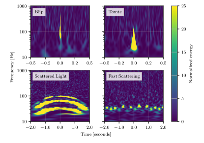
Figure 1: Time-frequency spectrograms of the four glitch classes which we analyse in this work.

To infer the properties of glitches in a given class, we first identify a list of glitch times pre-categorised by GravitySpy with a confidence threshold of 95%. We check that these glitches would typically contribute to the noise backgrounds estimated by search pipelines, i.e. they would not be vetoed by the single-detector signal-to-noise ratio (SNR) cuts; the details of this are given in the subsections of Sec. III. Each glitch is individually vetted by eye using a time-frequency visualisation to ensure it is consistent with the corresponding glitch class. We then analyse the data $\mathbf{d}_{i}$ surrounding the $i^{\rm th}$ glitch in our list using a stochastic sampling algorithm (specifically, the nested sampling dynesty [30] algorithm through the Bilby [31] package) and a model $M$. In this work, we use the IMRPhenomPv2 [32, 33] model which includes the inspiral, merger and ringdown of merging binary black holes and has been a standard benchmark waveform for several observing runs [34, 35]. IMRPhenomPv2, however, only models the dominant $(\ell,m)=(2,2)$ modes in the gravitational-wave radiation. Recent advances in waveform modelling have produced improved models, including the effect of higher-order modes [36, 37, 38, 39, 40, 41]. Nevertheless, we use IMRPhenomPv2 as it is well standardised and fast to evaluate, enabling us to analyse hundreds of glitches without a high computational cost. However, this implies that we infer the properties of glitches given the IMRPhenomPv2 waveform model. It is well known that systematic uncertainty exists between waveform models and that models including higher-order modes produce quite different posterior distributions, especially when the system has asymmetric masses [42, 43, 44]. We, therefore, caution when comparing the glitch population obtained herein with candidate triggers that are analysed using waveforms other than IMRPhenomPv2, especially if those waveforms include the effect of higher-order modes.

The IMRPhenomPv2 model has an associated set of model parameters $\theta$, which describe the mass, spins, location, and orientation of the source. For each glitch class, we produce an estimate of the posterior distribution $p(\theta|\mathbf{d}_{i},M)$ (in the form of a set of posterior samples) and the Bayesian evidence $\mathcal{Z}(\mathbf{d}_{i}|M)$. During the analysis of individual glitches, we use a Bayesian prior $\pi(\theta)$ appropriate for analysing astrophysical binary black holes. Specifically, the prior is uniform in the detector-frame chirp mass $\mathcal{M}^{\rm det}$ [45] between 8 and 200 $M_{\odot}$ and uniform in mass ratio $q$ between $1/20$ and 1 and assumes an isotropic distribution on the black holes spins. For all other parameters, we use the standard non-informative astrophysical prior distributions defined in Veitch et al. [46].

To infer the population properties of glitches in a given class, we take the set of posterior samples and Bayesian evidence from each individual analysis and perform a hierarchical population inference. Specifically, for a parameter $\theta_{i}\in\theta$, we define a population hyper-model $H$ with associated model hyperparameters $\Lambda$ such that we can evaluate $\pi(\theta_{i}|\Lambda,H)$. Once defined, we then utilise a variation on importance sampling to construct the likelihood $\mathcal{L}(\{\mathbf{d}_{i}|\Lambda,H)$. (We describe the population hypermodels and specifics of the likelihood used in this work below). Given this likelihood and a suitable hyperprior $\pi(\Lambda|H)$, we then use stochastic sampling to infer $p(\Lambda|\{\mathbf{d}\},H)$, the population hyperparameters conditioned on all glitches in the given class. For this analysis, we use the Bilby-MCMC [47] Markov-Chain Monte-Carlo sampling algorithm; we verify that both the dynesty and Bilby-MCMC samplers produce equivalent results, but that Bilby-MCMC is more efficient in this instance where only the posterior distribution and not the Bayesian evidence is of interest.

In principle, a hyper-model can predict the population behaviour for the full 15-dimensional parameter space $\theta$, including correlations between parameters. However, for a sub-set of parameters, we do not observe any population trends (e.g., the sky localisation of a population of glitch events tends to be isotropically distributed). We find that three parameters, the chirp mass $\mathcal{M}^{\rm det}$, mass ratio $q$, and the dimensionless spin-magnitude of the primary (heavier-mass) object $a_{1}$ are the primary indicators for the glitch classes considered in this work. We will build population models for each of these parameters independently. There is a weak correlation between these parameters, but we choose to infer their properties separately. This discards information about the correlation but greatly simplifies the population models. In future work, we will investigate whether including such correlations can produce a more accurate probabilistic model.

For other parameters, we do not observe strong trends in the population, except for the detector-frame luminosity distance, for which we observe a piling up of events at the lower bound (100 Mpc). The glitches selected for this analysis are, by design, loud glitches which pass a confidence threshold for categorisation by the GravitySpy (see Zevin et al. [16] for details). Hence, our set of glitches has an intrinsic selection bias in the loudness and hence luminosity distance. It is no surprise then that we observe a trend that all glitches tend to have small luminosity distances, as this is the dominant term in the signal amplitude and hence determines how “loud” a glitch is. We choose not to model the luminosity distance as we would need to properly calibrate the model for the intrinsic selection bias of our set of glitches. Other parameters, such as the system mass, may also be affected by the selection bias, but we model them nonetheless.

In this work, we will use three hypermodels to capture the broad-scale population properties of each glitch class for each parameter. These are three hypermodels from an infinite set of possible models. We arrived at these by studying the performance of a larger superset of hypermodels using posterior-predictive checks (described below). Where more complicated models failed to improve the posterior-predictive checks, we used simpler models. These hyper-models are designed to capture the broad features in a simple parameterised form. The three hypermodels are:

1. A power law distribution, it has a single hyperparameter $\Lambda=\{\alpha\}$ and density

   $$\pi(\theta_{i}|\alpha,H_{1})\propto\theta_{i}^{\alpha}\,,$$ (1)

   with bounds given by the physical bounds on $\theta_{i}$. This distribution is useful for modelling populations which tend to rail against the physical bounds (for example, the primary spin). For $\alpha$, we use a normally distributed prior with zero mean and a standard deviation of 5. This removes the requirement for an arbitrary upper bound on the magnitude while exponentially suppressing very large values.

2. A truncated skew-normal distribution [48, 49], it has three hyperparameters $\Lambda=\{\mu,\sigma,\kappa\}$ and density

   $$\pi(\theta_{i}|\mu,\sigma,\kappa,H_{2})=\frac{2}{\sigma}\phi\left(\frac{\theta_{i}-\mu}{\sigma}\right)\Phi\left(\kappa\frac{\theta_{i}-\mu}{\sigma}\right)$$ (2)

   where $\phi(x)$ is the standard normal probability density function and $\Phi(x)$ is the error function. We truncate the distribution again to the physical bounds on $\theta_{i}$. This distribution is useful for modelling unimodal populations with a distinct peak. We use a uniform prior for $\mu$ over the prior support on $\theta_{i}$, a normal prior for $\kappa$ with zero mean and a standard deviation of 10 and a truncated normal prior for $\sigma$ with standard deviation given by the maximum support on $\theta_{i}$.

3. A mixture-model of two normal distributions with five hyperparameters $\Lambda=\{\xi,\mu_{0},\sigma_{0},\mu_{1},\sigma_{1}\}$ and density

   $$\pi(\theta_{i}|\Lambda)=\frac{\xi}{\sigma_{0}}\phi\left(\frac{\theta_{i}-\mu_{0}}{\sigma_{0}}\right)+\frac{1-\xi}{\sigma_{1}}\phi\left(\frac{\theta_{i}-\mu_{1}}{\sigma_{1}}\right)\,.$$ (3)

   This is effective in modelling multi-modal distributions; we do not include a skew as this was found to be poorly constrained in the cases where the M3 model was required. As is done for the M2 model, we use a uniform prior for $\mu_{0}$ and $\mu_{1}$ and a truncated normal distribution for $\sigma_{0}$ and $\sigma_{1}$. For $\xi$, we apply a uniform prior on [0, 0.5].

For each model, the likelihood is constructed from Equation (32) of Thrane and Talbot [29] using “recycling”. This enables a two-step approach (first analysing individual events, then the population properties), which is critical to reducing the wall-time of the analysis. For each hyper-model, we report the median values of $p(\Lambda|\{\mathbf{d}_{i}\},H)$. These, together with the model descriptions above, constitute the core product of this work: simple parameterised models of glitches in the LIGO detectors.

To verify that the hyper-model captures the broad-scale features of the population, we use predictive posterior checking. First, to plot the “Measured” population, we bin each individual glitch-posterior in a histogram, then plot the mean and the $90\%$ credible interval (between 5% and 95%). This provides a summary of the population properties, which includes the variation in the individual posteriors. An example of this population visualisation can be seen in the right-hand column of Table 2: the “Measured” curve shows the mean (solid grey line) and 90% credible interval (filled grey region) for the population of Blip glitches across separate parameters. Second, to plot the “Predicted” population, we repeat the process above but simulate the individual posteriors from the population model. Specifically, we draw $\theta_{i}$ from $p(\theta_{i}|\Lambda^{\prime})$ (where $\Lambda^{\prime}$ is the median) then simulate a posterior and repeat the steps above. The simulated posterior is derived by randomly sampling a posterior from the “Measured” population and aligning its mean with a random draw from the posterior population distribution. This is a non-optimal method, but the alternative (simulating the signal predicted by the posterior population distribution in real detector noise unaffected by other transient noise and performing Bayesian inference) is too computationally demanding to be feasible. Examples of the resulting posterior predictive checks can be found in the right-hand column of Table 2: the “Predicted” curve shows the mean (solid orange line) and 90% credible (filled orange region) predicted by the hyper model across separate parameters. Here we see that the models capture the broad features (e.g. the number and location of modes and their width) but do not always capture the details (e.g. the Measured and Predicted curves do not overlap perfectly).

III Results

We now describe the results for each glitch class in the sections below. For each glitch class, we provide a table with a summary (the glitch model and median inferred population parameters) and the results of the posterior predictive checks. We also provide this information in a machine-readable table A [50]. For each model, we report the results of a single hypermodel. However, we fitted various models during development and used the posterior predictive checks as a qualitative guide to select the best fitting model.

III.1 Tomte glitches

In Table 1, we report the hypermodel, median, and posterior predictive checks for the population properties in $\mathcal{M}^{\rm det}$, $q$, and $a_{1}$ for Tomte glitches in the H1 and L1 detectors. For each detector, we analyse a set of 1000 Tomte glitches identified with GravitySpy.. The SNR of these glitches ranges from 7.7 to 74; the distribution is peaked with a median SNR of 21, but 90% of the Tomte glitches have an SNR less than 36. We also verify that we find similar conclusions about the properties when we downsample to 100 glitches; we use this, later on, to justify analysing smaller sets of the Fast Scattering and Scattered Light glitches.

For the chirp mass, the measured glitch population is unimodal with a peak at $\sim$75\text{\,}\mathrm{M}_{\odot}$$ and some positive skew. We fit the population using the M2 Skew-Normal distribution and find a qualitatively acceptable fit for both detector populations. However, the model under-predicts the rate of glitches with $\mathcal{M}^{\rm det}\sim[125,175]$ in the H1 detector. While the broad features are consistent between H1 and L1, the amount of skew is noticeably different, and Tomte glitches in the H1 detectors have chirp mass values up to $\sim 150$, while Tomte glitches in the L1 detector, $\mathcal{M}^{\rm det}\lesssim 125$.

For the mass ratio, the population is unimodal with some skew and the bulk of support on $q\lesssim 1/2$. We fit the mass ratio distribution using the M2 Skew Normal model and find a good qualitative fit in H1 and L1. As with the chirp mass, we note some qualitative differences between the H1 and L1 detectors with greater support in the H1 detectors for mass ratio’s up to 0.5, which is not seen in the L1 glitch population.

The primary spin, $a_{1}$ piles up at the extreme spin case $a_{1}=1$; we fit this using the M1 power-law model and find a reasonable agreement. However, we note a lack of events at the $a_{1}=1$ bound. Our fitted model does not capture this feature; however, it is sufficiently narrow that overall the model remains a reasonable fit. The power-law index $\alpha\sim 5-6$ provides a rough guide to the extent to which the spin “piles up”; this value is less extreme than in the Blip glitch population discussed shortly. For the spin, we do not observe significant differences between the H1 and L1 detector populations.

III.2 Blip glitches

In Table 2, we report the hypermodel, median, and posterior predictive checks for the population properties in $\mathcal{M}^{\rm det}$, $q$, and $a_{1}$ for Blip glitches in the H1 and L1 detectors. We analyse a set of 1000 Blip glitches in both H1 and L1 identified with GravitySpy. . The SNR of these glitches ranges from 7.5 to 47. The distribution peaks at the minimum bound, and 90% of the glitches have an SNR less than 20. We also verify that our results are robust when using only a subset of 100 randomly selected glitches.

The measured glitch population is unimodal for the chirp mass, with a peak at $\sim 25M_{\odot}$ and some positive skew. We find that the M1 Skew-Normal model provides a good qualitative fit. Comparing the measured and predicted posterior checks, the distribution means are well aligned, though the Skew-Normal under-predicts the density in the $40-60~{}M_{\odot}$ region.

For the mass ratio, the population is bimodal, with identical features found in both detectors. The bimodality originates from bimodal features observed in the posterior distributions of individual events. Though we see significant scatter in the shape of individual posteriors, averaging over multiple glitches, we observe similar distributions in both the H1 and L1 detectors indicating a common origin. The bulk of the support for both modes is found in the region $q\lesssim 1/2$, with some support up to the equal-mass bound. We apply the M3 normal mixture model, which provides a reasonable fit to the data, though it tends to underpredict the number of nearly equal-mass glitches in the L1 detector.

Finally, for $a_{1}$, the magnitude of the primary spin, we find that the measured glitch values pile up onto the extreme spin case $a_{1}\sim 1$. We also found this feature in the Tomte population, but here it is more extreme. We find the simplistic M1 power-law model provides a suitable fit to this data; the extreme power-law index $\alpha\sim 37$ demonstrates the strength of the pile-up.

Across all three parameters, we find remarkably consistent glitch behaviour between the H1 and L1 detectors. This, of course, may be simply due to the robust classification of events by GravitySpy. However, we note that the Tomte glitches did not show such consistency.

III.3 Fast Scattering glitches

In Table 3, we report the hypermodel, median, and posterior predictive checks for the population properties in $\mathcal{M}^{\rm det}$, $q$, and $a_{1}$ for Fast Scattering glitches in the H1 and L1 detectors. We use a set of 100 Fast Scattering glitches identified with GravitySpy. We limit ourselves to 100 glitches based on our analysis of the Blip and Tomte glitches, which indicated 100 glitches is sufficient to represent the population properties. This ten-fold reduction in events correspondingly reduces the computational burden of the analysis. The SNR distribution of these glitches is strongly peaked at the minimum bound of 7.5, with 90% of the glitches have an SNR less than 13. However, the distribution has a long tail with a maximum value of 121.

For the chirp mass, we find that the population has support from up to the artificial prior bound of . This indicates that the actual population likely have support at larger masses still. Such extreme heavy systems are beyond the space of likely astrophysical signals that ground-based detectors will observe in the advanced era. As such, extending our prior beyond this artificial bound is unlikely to help distinguish glitches from signals in the near term, so we choose not to do so. The observed distribution is “lumpy” with multiple components. We choose to fit the distribution with a Skew Normal distribution. This does not capture the “lumpy” behaviour but does broadly capture the typical support.

For the mass ratio, the Fast Scattering population have extreme mass ratios with a median of $\sim 1/10$ with some support up to $q\sim 0.8$. We fit this distribution using the M2 Skew Normal model and find a reasonable agreement between the predicted and measured distribution.

The primary spin, as with previously studied glitches, peaks at the extremal $a_{1}=1$ bound. However, the measured population has significant support for systems with $a_{1}$ right down to zero. We fit this distribution using the M1 power-law model and find a good fit.

III.4 Scattered light glitches

In Table 4, we report the hypermodel, median, and posterior predictive checks for the population properties in $\mathcal{M}^{\rm det}$, $q$, and $a_{1}$ for Scattered Light glitches in the H1 and L1 detectors. We use a set of 100 Scattered Light glitches identified with GravitySpy. The choice to use just 100 glitches mirrors the motivation in Sec. III.3. The SNR of these glitches ranges from 7.5 to 370; as with the Fast Scattering glitch type, the distribution peaks at the lower bound with a long tail. 90% of the glitches have an SNR less than 47.

For the chirp mass, we find that the population has support from up to the artificial prior bound of with significant “lumpiness”. The behaviour in the chirp mass distribution is similar in form between the Fast Scattering and Scattered Light glitches. For the L1 detector, there is a significant overabundance at the equal-mass bound. We choose to fit the distribution with a Skew Normal distribution. This does not capture the “lumpy” behaviour but does broadly capture the typical support.

For the mass ratio, the Scatter Light population have extreme mass ratios with a median of $\sim 1/10$. But, unlike the Scattered Light glitches, $q\lesssim 0.2$. We fit this distribution using the M2 Skew Normal model and find a reasonable agreement between the predicted and measured distribution.

As with previously studied glitches, the primary spin peaks at the extremal $a_{1}=1$ bound but with little support for smaller spins. We fit this distribution using the M1 power-law model and find a good fit. The power-law index $\alpha\sim 28$ is nearly as large as that of the Blip glitches.

IV Comparison with the GWTC2.1 catalogue

So far, 57 gravitational-wave signals have been reported and analysed by the LIGO, Virgo and KAGRA collaborations [34, 35, 52, 53]. Predominantly, these have been binary black hole systems (BBH) except for two binary neutron star (BNS) and two neutron star black hole (NSBH) binaries. Here we compare our glitch population with the 47 events with $p_{\rm astro}>0.5$ reported in either the GWTC2 [35] or GWTC2.1 [52] catalogues during the O3a observing run.

We provide two-dimensional plots comparing our glitch population with the observed signal in $\mathcal{M}^{\rm det}$-$q$ (Fig. 2), $\mathcal{M}^{\rm det}$-$a_{1}$ (Fig. 3), and $q$-$a_{1}$ (Fig. 4). In each plot, we give the 90% credible interval of the four glitch classes (for both H1 and L1) along with the combined equal-weighted glitch population in black. Projections of the overall glitch population are given for each one-dimensional plane. Overlaid on this, we then plot the symmetric 90% credible interval for all events with $p_{\rm astro}>0.5$ reported in either the GWTC2 or GWTC2.1 catalogues.

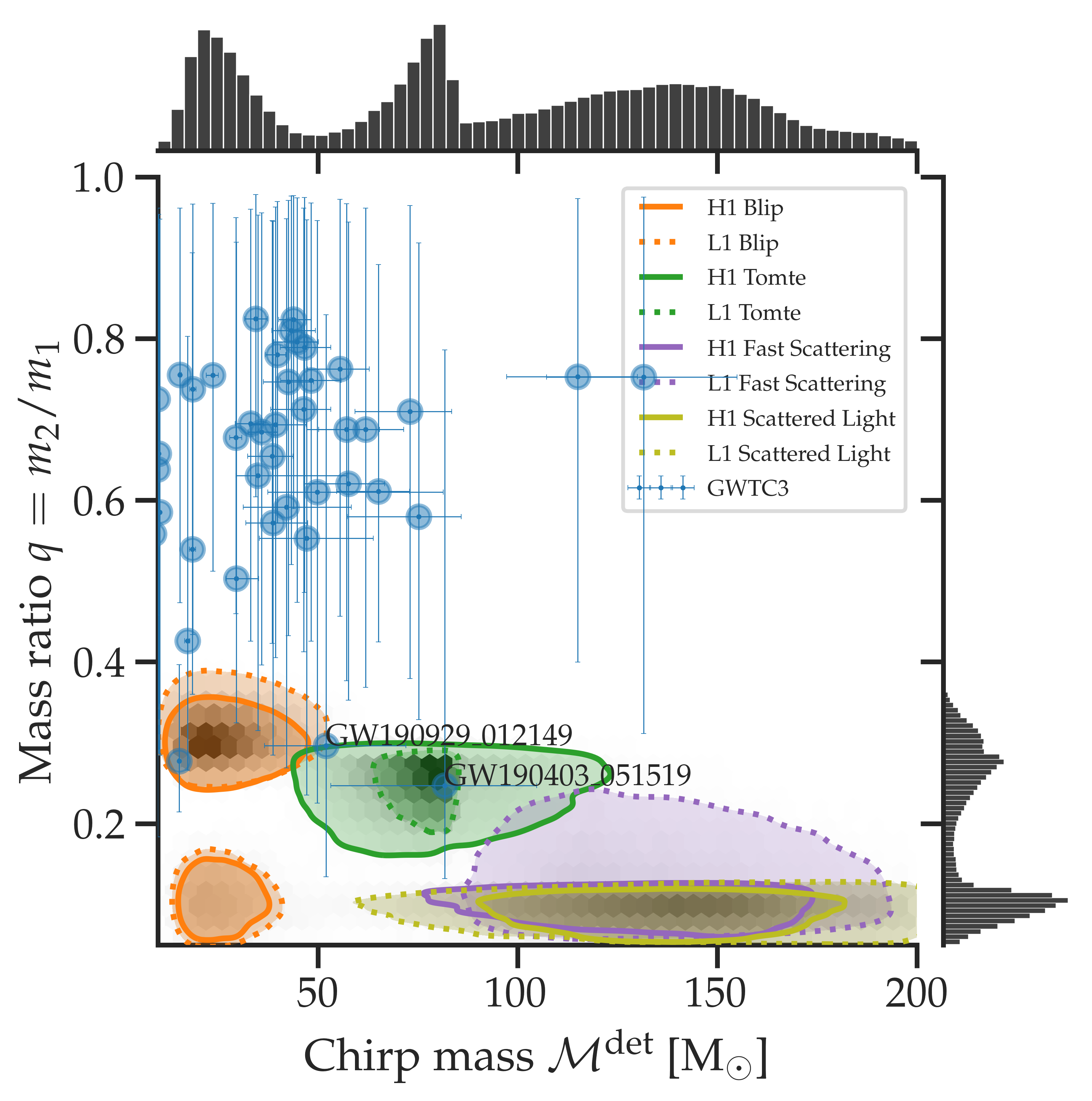
Figure 2: Visualisations of the parameterised glitch models developed in this work with the set of all events observed in the GWTC2 and GWTC2.1 catalogues [35, 52] for the chirp mass and mass ratio. A solid (dashed) line marks the 90% credible interval for the predicted distribution in the H1 (L1) detector, coloured by the glitch classification. A black density plot (and 1D marginal histograms) indicate the distribution of all glitches. Blue markers indicate all confident detections from the GWTC2 and GWTC2.1 catalogues. We remind the reader that the chirp mass reported here is measured in the red-shifted detector frame, not the source frame.

Figure 3: Visualisations of the parameterised glitch models developed in this work for the chirp mass and primary spin magnitude. See Fig. 2 for a complete description.

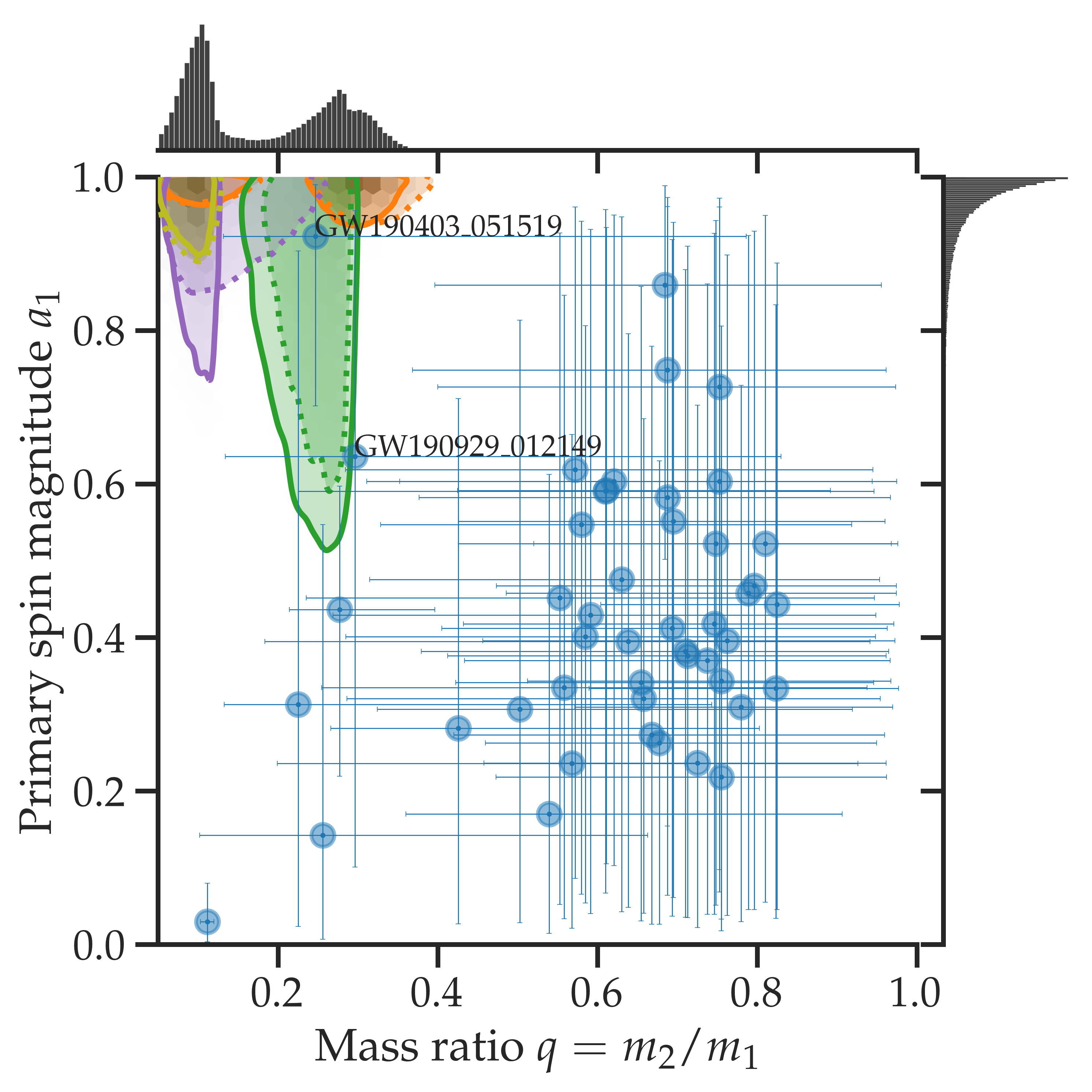
Figure 4: Visualisations of the parameterised glitch models developed in this work for the mass ratio and primary spin magnitude. See Fig. 2 for a complete description.

Comparing the glitch population with the astrophysical BBH distribution, three features stand out: $i)$ glitches have large spin magnitudes while astrophysical signals have median spin magnitudes $\lesssim 0.9$; $ii)$ glitches have extreme mass ratios while astrophysical signals tend to have more equal-mass; and finally, $iii)$, the combined glitch population spans the entire chirp mass range considered in this work, though individual glitch classes tend to cluster.

Glitches have extreme mass ratios and spin because the CBC signals models are a poor fit to the glitch morphology (see, e.g. Merritt et al. [25]). In the equal-mass zero-spin limit, the CBC waveform is sinusoidal with a characteristic monotonically increasing frequency evolution. Non-equal mass ratios and spins modify this behaviour introducing “twisting-up” effects which produce irregular waveform morphology’s. Glitches are caused by terrestrial disturbances, which are not expected to characteristically chirp up in frequency. So, when fitting the CBC signal model, it is unsurprising that the best fits happen in the non-equal mass and large spin limits.

Of the BBH systems reported so far in O3a, just one, GW190403_051519, falls firmly inside the 90% credible interval for the Tomte population in chirp mass, mass ratio, and primary spin magnitude. Additionally, GW190929_012149 sits at the edge of the Tomte distribution, but no signals are consistent with the other 3 glitch classes. Several other signals fall within the interval for the chirp mass and primary spin magnitude but are clearly distinguished when looking at the mass ratio and primary spin magnitude. However, it should be noted that both GW190403_051519 and GW190929_012149 have lower signal to noise ratios than any of the glitches included in our population analysis since we select only high-confidence glitches. However, Merritt et al. [25] argue that both quiet and loud glitches (of the same class) exhibit similar morphology.

In Fig. 5, we plot the time-frequency spectrogram of GW190403_051519 and a characteristic signal track. This illustrates that the event is primarily identified in the L1 detector, with no clear signal found in the H1 detector.

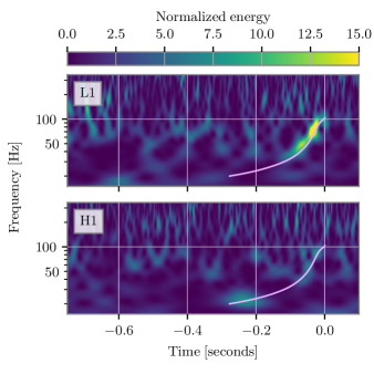
Figure 5: Time-frequency spectrograms of the GW190403_051519 event. We overlay the predicted signal using the SEOBNRv4_ROM waveform approximant [54] and the median-estimated signal properties from our IMRPhenomPv2 re-analysis of the event. (We note a mismatch between the waveform used for analysis and the waveform used to plot the signal track. However, the signal track here is intended only to guide the eye and not a quantitative test.)

GW190403_051519 was first identified in the GWTC2.1 catalogue by the GWTC2.1 PyCBC-BBH search alone [52] with a probability of astrophysical origin ($p_{\rm astro}$) of 0.61. No other pipelines identified GW190403_051519 as a candidate. Meanwhile, GW190929_012149 was identified in the GWTC2 catalogue by the GstLAL search alone [35] with $p_{\rm astro}$ =1. However, in the GWTC2.1 catalogue, GW190929_012149 was subsequently identified by all four pipelines used with $p_{\rm astro}$ values ranging from 0.14 to 0.87. GW190403_051519 is notable because the mass of the primary (heavier) object has more than 50% support for a mass greater than and is either inside or above the “mass gap” predicted by pair-instability supernova theory [55].

That GW190403_051519 and GW190929_012149 are consistent with the Tomte glitch population does not, of course, mean that the events are Tomte glitches. However, they have $p_{\rm astro}$ values, which allow for a terrestrial cause (i.e. $1-p_{\rm astro}\gtrsim 0.1$). Tomte glitches were numerous during O3a and are known to impact search sensitivity adversely. Therefore, it seems reasonable to conclude that if GW190403_051519 or GW190929_012149 are not of astrophysical origin, of the four glitch classes considered here, they are most consistent with Tomte glitches. However, we add that this assumes the signal morphology of the glitch classes studied herein extends to the low signal to noise ratio regime of GW190403_051519 and GW190929_012149.

This work does not change the estimated $p_{\rm astro}$ values for GW190403_051519 or GW190929_012149. The search pipelines that identify signals are robust to all relevant glitch classes, use information about the consistency between separate detectors, and apply glitch discriminators [15]. Using bootstrap approaches (e.g. time-shifting the data from independent detectors), the search pipelines estimate the background noise from all glitch classes, and this is intrinsically part of the $p_{\rm astro}$ calculation. Nevertheless, Fig. 4 does demonstrate that to identifying signals which have large spins and unequal mass ratios, astrophysical searches must contend with an elevated background of glitches compared to other areas of the parameter space. Search pipelines account for the distribution of noise triggers (including glitches) over the searched parameter space in their detection statistics and the resulting significance estimates (both the False Alarm Rate, FAR, and $p_{\rm astro}$), though this is done in a variety of ways [56, 14, 57, 13]. Therefore, the variation in glitch rate across the parameter space indicates that search pipelines are likely not uniformly sensitive across the parameter space [23, 58].

V Discussion and Conclusion

We present population models for the behaviour of non-Gaussian transient noise (glitches) in the Hanford and Livingston LIGO detectors during the O3a observing run. We first identify lists of Blip, Tomte, Fast Scattering, and Scattered light glitches pre-categorised by the GravitySpy citizen-science project and then vetted for class consistency using time-frequency visualisations. These glitch classes are known to most adversely search sensitivity. Using Bayesian inference, we then analyse each glitch class using a precessing binary black hole model. In effect, this allows us to project the properties of the glitch onto the parameter space of astrophysical signals. Finally, we use hierarchical population inference methods to fit simple parameterised models to the glitch populations. We do this separately for the chirp mass, mass ratio, and primary spin magnitude parameters; all other parameters we find to be only weakly informative at the population level. We verify the performance of the models using posterior predictive checks and confirm that they reproduce the bulk features of the population.

Finally, we compare the population of glitches with events observed with $p_{\rm astro}>0.5$ during the O3a observing run. We find two events, GW190403_051519 and GW190929_012149, which have a chirp mass, mass ratio, and primary spin magnitude consistent with the Tomte glitch class. GW190403_051519 is a fascinating case as it has a mass that may be inconsistent with the predictions of pair-instability supernova theory.

The parameterised models developed in this work could be used by search pipelines to potentially better distinguish astrophysical signals from terrestrial glitches . This could be implemented either additively in the detection statistic used by matched-filtering pipelines or as part of the astrophysical odds [24] (see [59] for the use of a simplistic glitch model). Already, many search pipelines use a version of this in which the detection statistics and background distributions are calculated over the template banks. This enables a lowering of the background rate in regions of parameter space less contaminated by glitches. Including the probabilistic models here into the detection statistic itself could refine this approach, providing more fine-grained modelled information. Ultimately, this may lead to a greater number of astrophysical signals being detected. However, the impact of this will depend on how much additional information is provided by these glitch models relative to the approaches already taken. To determine if such an approach can improve the detection efficiency, a large scale simulation study is needed, which is beyond the scope of the current work.

We also identify multimodality in the mass ratio of Blip glitches which may be used to identify this glitch class. We do not yet understand why this multimodality is exhibited, but it seems likely the waveform fits two separate parts of the glitch morphology in different regions of parameter space. This information may help formulate an improved glitch model (e.g., breaking the astrophysical waveform in a non-physical way that fits the glitch). Such a model could then be used to identify glitches and improve astrophysical searches.

At the same time, In the future, we hope to improve these models by including correlations between parameters, using higher-order mode waveform models and extending the study to sub-dominant parameters. These improvements will provide a more refined glitch consistency test and may reveal new glitch population features.

VI Acknowledgements

We a grateful to Derek Davis for help with the script used to produce Fig. 1 and Fig. 5, to Andrew Williamson for insightful comments about the nature of the bimodality seen in the Blip glitch mass ratio, to Tom Dent for helpful feedback on the manuscript, and to the CBC and detector characterisation groups of the LIGO and Virgo Collaborations for helpful feedback on this work. We also think Richard O’Shaughnessy, Jason Hathaway, Ben Henderson, Brian Cowburn for useful discussions related to this work. GA and LKN thank the UKRI Future Leaders Fellowship for support through the grant MR/T01881X/1. This research has made use of data, software and/or web tools obtained from the Gravitational Wave Open Science Center (https://www.gw-openscience.org), a service of LIGO Laboratory, the LIGO Scientific Collaboration and the Virgo Collaboration. LIGO is funded by the U.S. National Science Foundation. Virgo is funded by the French Centre National de Recherche Scientifique (CNRS), the Italian Istituto Nazionale della Fisica Nucleare (INFN) and the Dutch Nikhef, with contributions by Polish and Hungarian institutes. We are also grateful to computing resources provided by the LIGO Laboratory computing clusters at California Institute of Technology and LIGO Hanford Observatory supported by National Science Foundation Grants PHY-0757058 and PHY-0823459. The majority of analysis performed for this research was done using resources provided by the Open Science Grid [60, 61], which is supported by the National Science Foundation award #2030508. This work makes use of the scipy [62], numpy [63, 64, 65], gwpy [66], and PyCBC [12] software for data analysis and visualisation.

Detector	Type	Parameter	Model	Median	Posterior Predictive
H1	Tomte	$\mathcal{M}^{\rm det}$	M2: Skew-Normal	$\mu=56_{-1}^{+1}$ $\sigma=29_{-2}^{+2}$ $\kappa=3.6_{-0.6}^{+0.7}$
L1	Tomte	$\mathcal{M}^{\rm det}$	M2: Skew-Normal	$\mu=83.5_{-0.6}^{+0.6}$ $\sigma=8.8_{-0.6}^{+0.7}$ $\kappa=-10_{-10}^{+6}$
H1	Tomte	$q$	M2: Skew-Normal	$\mu=0.289_{-0.003}^{+0.003}$ $\sigma=0.057_{-0.003}^{+0.004}$ $\kappa=-14_{-10}^{+6}$
L1	Tomte	$q$	M2: Skew-Normal	$\mu=0.283_{-0.003}^{+0.003}$ $\sigma=0.043_{-0.003}^{+0.003}$ $\kappa=-16_{-10}^{+7}$
H1	Tomte	$a_{1}$	M1: Powerlaw	$\alpha=5.3_{-0.4}^{+0.4}$
L1	Tomte	$a_{1}$	M1: Powerlaw	$\alpha=6.9_{-0.6}^{+0.6}$

Table 1: Table of parameterised models for Tomte glitches in the H1 and L1 interferometers during the O3a era. Uncertainties on the median denote the symmetric 90% credible interval. See Sec. II for a description of the posterior predictive plots.

Detector	Type	Parameter	Model	Median	Posterior Predictive
H1	Blip	$\mathcal{M}^{\rm det}$	M2: Skew-Normal	$\mu=17.2_{-0.4}^{+0.5}$ $\sigma=11.8_{-0.6}^{+0.6}$ $\kappa=4.1_{-0.6}^{+0.7}$
L1	Blip	$\mathcal{M}^{\rm det}$	M2: Skew-Normal	$\mu=16.1_{-0.6}^{+0.6}$ $\sigma=14.7_{-0.8}^{+0.9}$ $\kappa=4.3_{-0.7}^{+0.8}$
H1	Blip	$q$	M3: Normal+Normal	$\mu_{0}=0.104_{-0.005}^{+0.005}$ $\sigma_{0}=0.030_{-0.003}^{+0.005}$ $\mu_{1}=0.299_{-0.002}^{+0.002}$ $\sigma_{1}=0.018_{-0.001}^{+0.002}$ $\xi=0.20_{-0.02}^{+0.03}$
L1	Blip	$q$	M3: Normal+Normal	$\mu_{0}=0.101_{-0.01}^{+0.006}$ $\sigma_{0}=0.038_{-0.005}^{+0.008}$ $\mu_{1}=0.317_{-0.002}^{+0.003}$ $\sigma_{1}=0.025_{-0.002}^{+0.002}$ $\xi=0.21_{-0.03}^{+0.03}$
H1	Blip	$a_{1}$	M1: Powerlaw	$\alpha=58_{-5}^{+4}$
L1	Blip	$a_{1}$	M1: Powerlaw	$\alpha=60_{-4}^{+5}$

Table 2: Table of parameterised models for Blip glitches in the H1 and L1 interferometers during the O3a era. Uncertainties on the median denote the symmetric 90% credible interval. See Sec. II for a description of the posterior predictive plots. See Sec. II for a description of the posterior predictive plots.

Detector	Type	Parameter	Model	Median	Posterior Predictive
H1	Fast Scattering	$\mathcal{M}^{\rm det}$	M2: Skew-Normal	$\mu=164_{-8}^{+7}$ $\sigma=39_{-6}^{+8}$ $\kappa=-7_{-10}^{+5}$
L1	Fast Scattering	$\mathcal{M}^{\rm det}$	M2: Skew-Normal	$\mu=102_{-8}^{+30}$ $\sigma=43_{-20}^{+10}$ $\kappa=4_{-4}^{+6}$
H1	Fast Scattering	$q$	M2: Skew-Normal	$\mu=0.120_{-0.009}^{+0.005}$ $\sigma=0.027_{-0.006}^{+0.006}$ $\kappa=-7_{-10}^{+6}$
L1	Fast Scattering	$q$	M2: Skew-Normal	$\mu=0.072_{-0.006}^{+0.006}$ $\sigma=0.077_{-0.02}^{+0.02}$ $\kappa=11_{-5}^{+10}$
H1	Fast Scattering	$a_{1}$	M3: Powerlaw	$\alpha=11_{-2}^{+3}$
L1	Fast Scattering	$a_{1}$	M3: Powerlaw	$\alpha=21_{-4}^{+6}$

Table 3: Table of parameterised models for Fast Scattering glitches in the H1 and L1 interferometers during the O3a era. Uncertainties on the median denote the symmetric 90% credible interval. See Sec. II for a description of the posterior predictive plots.

Detector	Type	Parameter	Model	Median	Posterior Predictive
H1	Scattered Light	$\mathcal{M}^{\rm det}$	M2: Skew-Normal	$\mu=151_{-30}^{+10}$ $\sigma=26_{-7}^{+9}$ $\kappa=-1_{-2}^{+2}$
L1	Scattered Light	$\mathcal{M}^{\rm det}$	M2: Skew-Normal	$\mu=199_{-10}^{+1}$ $\sigma=67_{-9}^{+9}$ $\kappa=-11_{-10}^{+8}$
H1	Scattered Light	$q$	M2: Skew-Normal	$\mu=0.113_{-0.006}^{+0.005}$ $\sigma=0.029_{-0.005}^{+0.005}$ $\kappa=-8_{-10}^{+5}$
L1	Scattered Light	$q$	M2: Skew-Normal	$\mu=0.116_{-0.05}^{+0.007}$ $\sigma=0.035_{-0.01}^{+0.008}$ $\kappa=-4_{-10}^{+6}$
H1	Scattered Light	$a_{1}$	M1: Powerlaw	$\alpha=29_{-5}^{+5}$
L1	Scattered Light	$a_{1}$	M1: Powerlaw	$\alpha=27_{-5}^{+6}$

Table 4: Table of parameterised models for scattered light glitches in the H1 and L1 interferometers during the O3a era. Uncertainties on the median denote the symmetric 90% credible interval.

References

- Aasi et al. [2015] J. Aasi et al., Advanced LIGO, Classical and Quantum Gravity 32, 074001 (2015), arXiv:1411.4547 [gr-qc] .
- Acernese et al. [2015] F. Acernese et al., Advanced Virgo: a second-generation interferometric gravitational wave detector, Classical and Quantum Gravity 32, 024001 (2015), arXiv:1408.3978 [gr-qc] .
- Aso et al. [2013] Y. Aso et al., Interferometer design of the KAGRA gravitational wave detector, Phys. Rev. D 88, 043007 (2013).
- Abbott et al. [2020a] B. P. Abbott et al., Prospects for observing and localizing gravitational-wave transients with Advanced LIGO, Advanced Virgo and KAGRA, Living Reviews in Relativity 23, 3 (2020a).
- Blackburn et al. [2008] L. Blackburn et al., The LSC glitch group: monitoring noise transients during the fifth LIGO science run, Classical and Quantum Gravity 25, 184004 (2008), arXiv:0804.0800 [gr-qc] .
- Abbott et al. [2016] B. P. Abbott et al., Characterization of transient noise in Advanced LIGO relevant to gravitational wave signal GW150914, Classical and Quantum Gravity 33, 134001 (2016), arXiv:1602.03844 [gr-qc] .
- Cabero et al. [2019] M. Cabero, A. Lundgren, A. H. Nitz, T. Dent, D. Barker, E. Goetz, J. S. Kissel, L. K. Nuttall, P. Schale, R. Schofield, et al., Blip glitches in Advanced LIGO data, Classical and Quantum Gravity 36, 155010 (2019), arXiv:1901.05093 [physics.ins-det] .
- Abbott et al. [2020b] B. P. Abbott et al., A guide to LIGO-Virgo detector noise and extraction of transient gravitational-wave signals, Classical and Quantum Gravity 37, 055002 (2020b), arXiv:1908.11170 [gr-qc] .
- Davis et al. [2021] D. Davis et al., LIGO detector characterization in the second and third observing runs, Classical and Quantum Gravity 38, 135014 (2021), arXiv:2101.11673 [astro-ph.IM] .
- Allen et al. [2012] B. Allen, W. G. Anderson, P. R. Brady, D. A. Brown, and J. D. E. Creighton, FINDCHIRP: An algorithm for detection of gravitational waves from inspiraling compact binaries, Phys. Rev. D 85, 122006 (2012), arXiv:gr-qc/0509116 [gr-qc] .
- Cannon et al. [2013] K. Cannon, C. Hanna, and D. Keppel, Method to estimate the significance of coincident gravitational-wave observations from compact binary coalescence, Phys. Rev. D 88, 024025 (2013), arXiv:1209.0718 [gr-qc] .
- Nitz et al. [2017] A. H. Nitz, T. Dent, T. Dal Canton, S. Fairhurst, and D. A. Brown, Detecting Binary Compact-object Mergers with Gravitational Waves: Understanding and Improving the Sensitivity of the PyCBC Search, Astrophys. J. 849, 118 (2017), arXiv:1705.01513 [gr-qc] .
- Aubin et al. [2021] F. Aubin, F. Brighenti, R. Chierici, D. Estevez, G. Greco, G. M. Guidi, V. Juste, F. Marion, B. Mours, E. Nitoglia, et al., The MBTA pipeline for detecting compact binary coalescences in the third LIGO-Virgo observing run, Classical and Quantum Gravity 38, 095004 (2021), arXiv:2012.11512 [gr-qc] .
- Sachdev et al. [2019] S. Sachdev et al., The GstLAL Search Analysis Methods for Compact Binary Mergers in Advanced LIGO’s Second and Advanced Virgo’s First Observing Runs, arXiv e-prints , arXiv:1901.08580 (2019), arXiv:1901.08580 [gr-qc] .
- Allen [2005] B. Allen, 2 time-frequency discriminator for gravitational wave detection, Phys. Rev. D 71, 062001 (2005), arXiv:gr-qc/0405045 [gr-qc] .
- Zevin et al. [2017] M. Zevin et al., Gravity Spy: integrating advanced LIGO detector characterization, machine learning, and citizen science, Classical and Quantum Gravity 34, 064003 (2017), arXiv:1611.04596 [gr-qc] .
- Mukherjee et al. [2010] S. Mukherjee, R. Obaid, and B. Matkarimov, Classification of glitch waveforms in gravitational wave detector characterization, in Journal of Physics Conference Series, Journal of Physics Conference Series, Vol. 243 (2010) p. 012006.
- Rampone et al. [2013] S. Rampone, V. Pierro, L. Troiano, and I. M. Pinto, Neural Network Aided Glitch-Burst Discrimination and Glitch Classification, International Journal of Modern Physics C 24, 1350084 (2013), arXiv:1401.5941 [astro-ph.IM] .
- Powell et al. [2015] J. Powell, D. Trifirò, E. Cuoco, I. S. Heng, and M. Cavaglià, Classification methods for noise transients in advanced gravitational-wave detectors, Classical and Quantum Gravity 32, 215012 (2015), arXiv:1505.01299 [astro-ph.IM] .
- Powell et al. [2017] J. Powell, A. Torres-Forné, R. Lynch, D. Trifirò, E. Cuoco, M. Cavaglià, I. S. Heng, and J. A. Font, Classification methods for noise transients in advanced gravitational-wave detectors II: performance tests on Advanced LIGO data, Classical and Quantum Gravity 34, 034002 (2017), arXiv:1609.06262 [astro-ph.IM] .
- Mukund et al. [2017] N. Mukund, S. Abraham, S. Kandhasamy, S. Mitra, and N. S. Philip, Transient classification in LIGO data using difference boosting neural network, Phys. Rev. D 95, 104059 (2017), arXiv:1609.07259 [astro-ph.IM] .
- Jadhav et al. [2020] S. Jadhav, N. Mukund, B. Gadre, S. Mitra, and S. Abraham, Improving significance of binary black hole mergers in Advanced LIGO data using deep learning : Confirmation of GW151216, arXiv e-prints , arXiv:2010.08584 (2020), arXiv:2010.08584 [gr-qc] .
- Davis et al. [2020] D. Davis, L. V. White, and P. R. Saulson, Utilizing aLIGO glitch classifications to validate gravitational-wave candidates, Classical and Quantum Gravity 37, 145001 (2020), arXiv:2002.09429 [gr-qc] .
- Ashton et al. [2019a] G. Ashton, E. Thrane, and R. J. E. Smith, Gravitational wave detection without boot straps: A Bayesian approach, Phys. Rev. D 100, 123018 (2019a), arXiv:1909.11872 [gr-qc] .
- Merritt et al. [2021] J. Merritt, B. Farr, R. Hur, B. Edelman, and Z. Doctor, Transient glitch mitigation in Advanced LIGO data with glitschen, arXiv e-prints , arXiv:2108.12044 (2021), arXiv:2108.12044 [gr-qc] .
- Mandel [2010] I. Mandel, Parameter estimation on gravitational waves from multiple coalescing binaries, Phys. Rev. D 81, 084029 (2010), arXiv:0912.5531 [astro-ph.HE] .
- Mandel and O’Shaughnessy [2010] I. Mandel and R. O’Shaughnessy, Compact binary coalescences in the band of ground-based gravitational-wave detectors, Classical and Quantum Gravity 27, 114007 (2010), arXiv:0912.1074 [astro-ph.HE] .
- Adams et al. [2012] M. R. Adams, N. J. Cornish, and T. B. Littenberg, Astrophysical model selection in gravitational wave astronomy, Phys. Rev. D 86, 124032 (2012), arXiv:1209.6286 [gr-qc] .
- Thrane and Talbot [2019] E. Thrane and C. Talbot, An introduction to Bayesian inference in gravitational-wave astronomy: Parameter estimation, model selection, and hierarchical models, Publications of the Astronomical Society of Australia 36, e010 (2019), arXiv:1809.02293 [astro-ph.IM] .
- Speagle [2020] J. S. Speagle, DYNESTY: a dynamic nested sampling package for estimating Bayesian posteriors and evidences, Monthly Notices of the Royal Astronomical Society 493, 3132 (2020), arXiv:1904.02180 [astro-ph.IM] .
- Ashton et al. [2019b] G. Ashton et al., BILBY: A User-friendly Bayesian Inference Library for Gravitational-wave Astronomy, APJS 241, 27 (2019b), arXiv:1811.02042 [astro-ph.IM] .
- Hannam et al. [2014] M. Hannam, P. Schmidt, A. Bohé, L. Haegel, S. Husa, F. Ohme, G. Pratten, and M. Pürrer, Simple Model of Complete Precessing Black-Hole-Binary Gravitational Waveforms, Phys. Rev. Lett. 113, 151101 (2014), arXiv:1308.3271 [gr-qc] .
- Schmidt et al. [2012] P. Schmidt, M. Hannam, and S. Husa, Towards models of gravitational waveforms from generic binaries: A simple approximate mapping between precessing and nonprecessing inspiral signals, Phys. Rev. D 86, 104063 (2012).
- Abbott et al. [2019] B. P. Abbott et al., GWTC-1: A Gravitational-Wave Transient Catalog of Compact Binary Mergers Observed by LIGO and Virgo during the First and Second Observing Runs, Physical Review X 9, 031040 (2019), arXiv:1811.12907 [astro-ph.HE] .
- Abbott et al. [2021a] R. Abbott et al., GWTC-2: Compact Binary Coalescences Observed by LIGO and Virgo during the First Half of the Third Observing Run, Physical Review X 11, 021053 (2021a), arXiv:2010.14527 [gr-qc] .
- London et al. [2018] L. London, S. Khan, E. Fauchon-Jones, C. García, M. Hannam, S. Husa, X. Jiménez-Forteza, C. Kalaghatgi, F. Ohme, and F. Pannarale, First Higher-Multipole Model of Gravitational Waves from Spinning and Coalescing Black-Hole Binaries, Phys. Rev. Lett. 120, 161102 (2018), arXiv:1708.00404 [gr-qc] .
- Cotesta et al. [2018] R. Cotesta, A. Buonanno, A. Bohé, A. Taracchini, I. Hinder, and S. Ossokine, Enriching the symphony of gravitational waves from binary black holes by tuning higher harmonics, Phys. Rev. D 98, 084028 (2018), arXiv:1803.10701 [gr-qc] .
- Nagar et al. [2018] A. Nagar et al., Time-domain effective-one-body gravitational waveforms for coalescing compact binaries with nonprecessing spins, tides, and self-spin effects, Phys. Rev. D 98, 104052 (2018), arXiv:1806.01772 [gr-qc] .
- Varma et al. [2019] V. Varma, S. E. Field, M. A. Scheel, J. Blackman, L. E. Kidder, and H. P. Pfeiffer, Surrogate model of hybridized numerical relativity binary black hole waveforms, Phys. Rev. D 99, 064045 (2019), arXiv:1812.07865 [gr-qc] .
- Pratten et al. [2021] G. Pratten, C. García-Quirós, M. Colleoni, A. Ramos-Buades, H. Estellés, M. Mateu-Lucena, R. Jaume, M. Haney, D. Keitel, J. E. Thompson, et al., Computationally efficient models for the dominant and subdominant harmonic modes of precessing binary black holes, Phys. Rev. D 103, 104056 (2021), arXiv:2004.06503 [gr-qc] .
- Estellés et al. [2020] H. Estellés, S. Husa, M. Colleoni, D. Keitel, M. Mateu-Lucena, C. García-Quirós, A. Ramos-Buades, and A. Borchers, Time domain phenomenological model of gravitational wave subdominant harmonics for quasi-circular non-precessing binary black hole coalescences, arXiv e-prints , arXiv:2012.11923 (2020), arXiv:2012.11923 [gr-qc] .
- Abbott [2020] R. o. Abbott, GW190412: Observation of a binary-black-hole coalescence with asymmetric masses, Phys. Rev. D 102, 043015 (2020).
- Abbott et al. [2020c] R. Abbott et al., GW190521: A Binary Black Hole Merger with a Total Mass of 150 M⊙, Phys. Rev. Lett. 125, 101102 (2020c), arXiv:2009.01075 [gr-qc] .
- Abbott et al. [2020d] R. Abbott et al., GW190814: Gravitational Waves from the Coalescence of a 23 Solar Mass Black Hole with a 2.6 Solar Mass Compact Object, APJL 896, L44 (2020d), arXiv:2006.12611 [astro-ph.HE] .
- Cutler and Flanagan [1994] C. Cutler and E. E. Flanagan, Gravitational waves from merging compact binaries: How accurately can one extract the binary’s parameters from the inspiral waveform?, Phys. Rev. D 49, 2658 (1994).
- Veitch et al. [2015] J. Veitch et al., Parameter estimation for compact binaries with ground-based gravitational-wave observations using the LALInference software library, Phys. Rev. D 91, 042003 (2015), arXiv:1409.7215 [gr-qc] .
- Ashton and Talbot [2021] G. Ashton and C. Talbot, BILBY-MCMC: an MCMC sampler for gravitational-wave inference, Monthly Notices of the Royal Astronomical Society 507, 2037 (2021), arXiv:2106.08730 [gr-qc] .
- O’hagan and Leonard [1976] A. O’hagan and T. Leonard, Bayes estimation subject to uncertainty about parameter constraints, Biometrika 63, 201 (1976).
- Azzalini and Capitanio [1999] A. Azzalini and A. Capitanio, Statistical applications of the multivariate skew normal distribution, Journal of the Royal Statistical Society: Series B (Statistical Methodology) 61, 579 (1999).
- Ashton [2021] G. Ashton, Data release: Parameterised population models of transient non-Gaussian noise in the LIGO gravitational-wave detectors, 10.5281/zenodo.5550510 (2021).
- Robinet et al. [2020] F. Robinet, N. Arnaud, N. Leroy, A. Lundgren, D. Macleod, and J. McIver, Omicron: A tool to characterize transient noise in gravitational-wave detectors, SoftwareX 12, 100620 (2020), arXiv:2007.11374 [astro-ph.IM] .
- The LIGO Scientific Collaboration et al. [2021] The LIGO Scientific Collaboration, the Virgo Collaboration, et al., GWTC-2.1: Deep Extended Catalog of Compact Binary Coalescences Observed by LIGO and Virgo During the First Half of the Third Observing Run, arXiv e-prints , arXiv:2108.01045 (2021), arXiv:2108.01045 [gr-qc] .
- Abbott et al. [2021b] R. Abbott et al., Observation of Gravitational Waves from Two Neutron Star-Black Hole Coalescences, APJL 915, L5 (2021b), arXiv:2106.15163 [astro-ph.HE] .
- Bohé et al. [2017] A. Bohé, L. Shao, A. Taracchini, A. Buonanno, S. Babak, I. W. Harry, I. Hinder, S. Ossokine, M. Pürrer, V. Raymond, et al., Improved effective-one-body model of spinning, nonprecessing binary black holes for the era of gravitational-wave astrophysics with advanced detectors, Phys. Rev. D 95, 044028 (2017), arXiv:1611.03703 [gr-qc] .
- Woosley [2017] S. E. Woosley, Pulsational Pair-instability Supernovae, Astrophys. J. 836, 244 (2017), arXiv:1608.08939 [astro-ph.HE] .
- Nitz et al. [2019] A. H. Nitz, C. Capano, A. B. Nielsen, S. Reyes, R. White, D. A. Brown, and B. Krishnan, 1-OGC: The first open gravitational-wave catalog of binary mergers from analysis of public advanced LIGO data, The Astrophysical Journal 872, 195 (2019).
- Nitz et al. [2020] A. H. Nitz, T. Dent, G. S. Davies, S. Kumar, C. D. Capano, I. Harry, S. Mozzon, L. Nuttall, A. Lundgren, and M. Tápai, 2-OGC: Open gravitational-wave catalog of binary mergers from analysis of public advanced LIGO and virgo data, The Astrophysical Journal 891, 123 (2020).
- Abbott et al. [2018] B. P. Abbott et al., Effects of data quality vetoes on a search for compact binary coalescences in Advanced LIGO’s first observing run, Classical and Quantum Gravity 35, 065010 (2018), arXiv:1710.02185 [gr-qc] .
- Ashton and Thrane [2020] G. Ashton and E. Thrane, The astrophysical odds of GW151216, Monthly Notices of the Royal Astronomical Society 498, 1905 (2020), arXiv:2006.05039 [astro-ph.HE] .
- Pordes et al. [2007] R. Pordes, D. Petravick, B. Kramer, D. Olson, M. Livny, A. Roy, P. Avery, K. Blackburn, T. Wenaus, F. Würthwein, et al., The open science grid, in J. Phys. Conf. Ser., 78, Vol. 78 (2007) p. 012057.
- Sfiligoi et al. [2009] I. Sfiligoi, D. C. Bradley, B. Holzman, P. Mhashilkar, S. Padhi, and F. Wurthwein, The pilot way to grid resources using glideinwms, in 2009 WRI World Congress on Computer Science and Information Engineering, 2, Vol. 2 (2009) pp. 428–432.
- Virtanen et al. [2020] P. Virtanen, R. Gommers, T. E. Oliphant, M. Haberland, T. Reddy, D. Cournapeau, E. Burovski, P. Peterson, W. Weckesser, J. Bright, et al., SciPy 1.0: Fundamental Algorithms for Scientific Computing in Python, Nature Methods 17, 261 (2020).
- Oliphant [2006] T. E. Oliphant, A guide to NumPy, Vol. 1 (Trelgol Publishing USA, 2006).
- Van Der Walt et al. [2011] S. Van Der Walt, S. C. Colbert, and G. Varoquaux, The numpy array: a structure for efficient numerical computation, Computing in Science & Engineering 13, 22 (2011).
- Harris et al. [2020] C. R. Harris, K. J. Millman, S. J. van der Walt, R. Gommers, P. Virtanen, D. Cournapeau, E. Wieser, J. Taylor, S. Berg, N. J. Smith, et al., Array programming with numpy, Nature 585, 357 (2020).
- Macleod et al. [2021] D. Macleod, A. L. Urban, S. Coughlin, T. Massinger, M. Pitkin, and rngeorge, gwpy/gwpy: 2.0.3 (2021).