Nematic quantum criticality in Dirac systems

Abstract

We investigate nematic quantum phase transitions in two different Dirac fermion models. The models feature twofold and fourfold, respectively, lattice rotational symmetries that are spontaneously broken in the ordered phase. Using negative-sign-free quantum Monte Carlo simulations and an $\epsilon$-expansion renormalization group analysis, we show that both models exhibit continuous phase transitions. In contrast to generic Gross-Neveu dynamical mass generation, the quantum critical regime is characterized by large velocity anisotropies, with fixed-point values being approached very slowly. Both experimental and numerical investigations will not be representative of the infrared fixed point, but of a quasiuniversal regime where the drift of the exponents tracks the velocity anisotropy.

In a strongly correlated electron system, global symmetries, such as spin rotation, point group, or translational symmetries, can be spontaneously broken as a function of some external tuning parameter. This challenging problem has been studied extensively numerically and experimentally over the last years and impacts our understanding of quantum criticality [1] in cuprates [2] and heavy fermions [3]. The problem greatly simplifies when the Fermi surface reduces to isolated Fermi points in $2+1$ dimensions and the critical point features emergent Lorentz symmetry. In this context, spin, time reversal, and translational symmetry breaking generically correspond to the dynamical generation of mass terms [4], and the semimetal-to-insulator transition belongs to one of the various Gross-Neveu universality classes [5, 6, 7, 8, 9, 10, 11].

Across nematic transitions, rotational symmetry is spontaneously broken [12, 13]. For continuum Dirac fermions with Hamiltonian $H(\bm{k})=v\left(k_{x}\sigma_{x}+k_{y}\sigma_{y}\right)$ in momentum space, where $\bm{\sigma}$ are Pauli spin matrices and $v$ is the Fermi velocity, nematic transitions correspond to the dynamical generation of nonmass terms, such as $m\sigma_{x}$. They shift the position of the Dirac cone and as such break rotational, and therewith also Lorentz, symmetries. Such nematic transitions have been studied theoretically in the past in the context of $d$-wave superconductors [14, 15, 16, 17, 18] and bilayer graphene [19]. Fundamental questions pertaining to the very nature of the transition remain open: While initial renormalization group (RG) calculations based on the $\epsilon$ expansion suggested a first-order transition [14, 15], a continuous transition has been found in large-$N$ analyses [17, 16]. In this Letter, we use quantum Monte Carlo (QMC) simulations and a revised $\epsilon$-expansion analysis to study these transitions. We introduce two different models of Dirac fermions with twofold and fourfold, respectively, lattice rotational symmetries and demonstrate numerically and analytically that both models feature a continuous nematic transition, realizing a new family of quantum universality classes in Dirac systems without emergent Lorentz invariance.

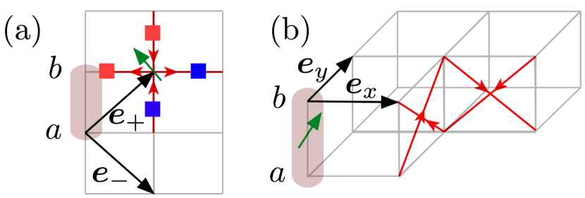
Figure 1: Sketch of (a) $C_{2v}$ and (b) $C_{4v}$ models, defined on $\pi$-flux single-layer and bilayer square lattices, with lattice vectors $\bm{e}_{\nicefrac{{+}}{{-}}}$ and $\bm{e}_{\nicefrac{{x}}{{y}}}$, respectively. Dark pink regions indicate unit cells, containing two orbitals ($a$ and $b$) and one Ising spin (green arrow) in both cases. Fermions hop along the red lines and acquire a phase factor $e^{i\pi/4}$ when following the direction of the arrow. Red and blue squares in (a) indicate the sign structure in the Yukawa coupling of the $C_{2v}$ model.

Models.

Inspired from Refs. [13, 20, 21], we design two models of (2+1)-dimensional Dirac fermions, $\mathcal{H}_{0}$, coupled to a transverse-field Ising model (TFIM),

$$\mathcal{H}_{\text{Ising}}=-J\sum_{\langle\bm{R},\bm{R}^{\prime}\rangle}\hat{s}_{\bm{R}}^{z}\hat{s}_{\bm{R}^{\prime}}^{z}-h\sum_{\bm{R}}\hat{s}_{\bm{R}}^{x},$$ (1)

where $\bm{R}$ denotes a unit cell and $\langle\bm{R},\bm{R}^{\prime}\rangle$ runs over adjacent unit cells. A Yukawa coupling, $\mathcal{H}_{\text{Yuk}}$, between the Ising field and nematic fermion bilinear yields the desired models, $\mathcal{H}=\mathcal{H}_{0}+\mathcal{H}_{\text{Ising}}+\mathcal{H}_{\text{Yuk}}$, that correspond to one of many possible lattice regularizations of continuum field theories of Eqs. (4) and (Continuum field theory.).

In the $C_{2v}$ model, depicted in Fig. 1(a), we employ a $\pi$-flux Hamiltonian on the square lattice as

$$\mathcal{H}_{0}^{C_{2v}} =-t\sum_{\bm{R}}\sum_{\sigma=1}^{N_{\sigma}}\hat{a}_{\bm{R},\sigma}^{\dagger}\Big{(}\hat{b}_{\bm{R},\sigma}\mathrm{e}^{-i\tfrac{\pi}{4}}+\hat{b}_{\bm{R}+\bm{e}_{-},\sigma}\mathrm{e}^{i\tfrac{\pi}{4}}$$

$$\quad+\hat{b}_{\bm{R}+\bm{e}_{-}-\bm{e}_{+},\sigma}\mathrm{e}^{-i\tfrac{\pi}{4}}+\hat{b}_{\bm{R}-\bm{e}_{+},\sigma}\mathrm{e}^{i\tfrac{\pi}{4}}\Big{)}+\mathrm{H.c.},$$ (2a)

where $$\hat{a} \hat{b} \sigma t N_{\sigma}=2 \mathcal{H}_{0} \hat{s}_{\bm{R}}$$ and with spin index are fermion annihilation operators on the two sublattices, is the hopping parameter, and is the number of spin degrees of freedom. features two inequivalent Dirac points per spin component in the Brillouin zone (BZ). The Ising spins couple, with the sign structure indicated in Fig. 1(a), to the nearest-neighbor fermion hopping terms,

$$\mathcal{H}_{\text{Yuk}}^{C_{2v}} =-\xi\sum_{\bm{R}}\sum_{\sigma=1}^{N_{\sigma}}\hat{s}_{\bm{R}}^{z}\hat{a}^{\dagger}_{\bm{R},\sigma}\Big{(}\hat{b}_{\bm{R},\sigma}\mathrm{e}^{-i\tfrac{\pi}{4}}-\hat{b}_{\bm{R}+\bm{e}_{-},\sigma}\mathrm{e}^{i\tfrac{\pi}{4}}$$

$$\quad-\hat{b}_{\bm{R}+\bm{e}_{-}-\bm{e}_{+},\sigma}\mathrm{e}^{-i\tfrac{\pi}{4}}+\hat{b}_{\bm{R}-\bm{e}_{+},\sigma}\mathrm{e}^{i\tfrac{\pi}{4}}\Big{)}+\mathrm{H.c.},$$ (2b)

where $\xi$ denotes the coupling strength. The model has a $C_{2v}$ point group symmetry, composed of reflections, $\hat{T}_{\pm}$ on the $\bm{e}_{\pm}=\bm{e}_{x}\pm\bm{e}_{y}$ axis. $\hat{T}_{\pm}$ pins the Dirac cones to the $\bm{K}_{\pm}=(\pi/2,\pm\pi/2)$ points in the BZ. Aside from the above reflections, $\pi$ rotations about the $z$ axis are obtained as $\hat{T}_{+}\hat{T}_{-}$. Further, the model exhibits an explicit $\text{SU}(N_{\sigma})$ spin symmetry that is enlarged to $O(2N_{\sigma})$ [22].

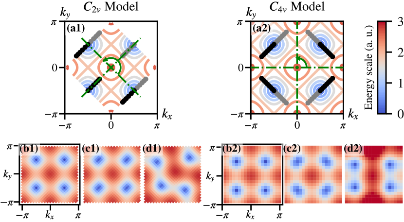
Figure 2: (a) Contour plot of the fermion dispersion in the disordered phase from mean-field theory. The green lines and arrows indicate the point group symmetries. Black (gray) dots sketch the meandering of the Dirac cones in the nematic phase for $\langle\hat{s}_{\bm{R}}^{z}\rangle>0$ ($<0$). (b)-(d) Fermion dispersion from QMC at $L=20$ for (b) $h=5.0>h_{c}$ featuring isotropic Fermi velocities (c) $h\simeq h_{c}$, $h\approx 3.27$ (left) and $h\approx 3.65$ (right), and (d) at $h=1.0<h_{c}$ featuring broken point-group symmetries. Color scale applies to all plots.

The $C_{4v}$ model corresponds to a bilayer $\pi$-flux model, in which the Ising spins are located on the rungs, Fig. 1(b). The fermion hopping Hamiltonian is

$$\mathcal{H}_{0}^{C_{4v}} =-t\sum_{\bm{R}}\sum_{\sigma=1}^{N_{\sigma}}\hat{a}_{\bm{R},\sigma}^{\dagger}\Big{(}\hat{b}_{\bm{R}+\bm{e}_{x},\sigma}\mathrm{e}^{i\tfrac{\pi}{4}}+\hat{b}_{\bm{R}-\bm{e}_{x},\sigma}\mathrm{e}^{i\tfrac{\pi}{4}}$$

$$\quad+\hat{b}_{\bm{R}+\bm{e}_{y},\sigma}\mathrm{e}^{-i\tfrac{\pi}{4}}+\hat{b}_{\bm{R}-\bm{e}_{y},\sigma}\mathrm{e}^{-i\tfrac{\pi}{4}}\Big{)}+\mathrm{H.c.},$$ (3a)

featuring four Dirac cones per spin component. The Yukawa coupling reads

$$\mathcal{H}_{\text{Yuk}}^{C_{4v}} =-\xi\sum_{\bm{R}}\sum_{\sigma=1}^{N_{\sigma}}i\hat{s}_{\bm{R}}^{z}\hat{a}^{\dagger}_{\bm{R},\sigma}\hat{b}_{\bm{R},\sigma}+\mathrm{H.c.},$$ (3b)

amounting to a coupling of the Ising spins to the interlayer fermion current. The $C_{4v}$ Hamiltonian commutes with $\hat{T}_{\pi/2}$, corresponding to $\pi/2$ rotation about the $z$ axis. The model is invariant under reflections $\hat{T}_{x}$ and $\hat{T}_{y}$ along the $x$ and $y$ axes, respectively. Reflections along $\bm{e}_{\pm}=\bm{e}_{x}\pm\bm{e}_{y}$, denoted by $\hat{T}_{\pm}$, can be derived from $\hat{T}_{\pi/2}$, $\hat{T}_{x}$, and $\hat{T}_{y}$, and therefore also leave the model invariant. The model hence has a $C_{4v}$ symmetry. Particle-hole symmetry, imposes $A(\bm{k},\omega)=A(-\bm{k}+\bm{Q},-\omega)$, where $\bm{Q}=(\pi,\pi)$ such that alongside with the $C_{4v}$ symmetry the Dirac cones are pinned to the $\pm\bm{K}_{\pm}$ points in the BZ [22].

Lattice mean-field theory.

The key point of both models is that the point group and particle-hole symmetries are tied to the flipping of the Ising spin degree of freedom. In the large-$h$ limit, the ground state has the full symmetry of the model Hamiltonian and at the mean-field level we can set $\langle\hat{s}_{\bm{R}}^{z}\rangle=0$. In this limit, the Dirac cones are pinned by symmetry. In the opposite small-$h$ limit, the Ising spins order, $\langle\hat{s}_{\bm{R}}^{z}\rangle\neq 0$. Thereby, the $C_{2v}$ ($C_{4v}$) symmetry is reduced to $\hat{T}_{+}$ ($C_{2v}$). At the mean-field level, this induces a meandering of the Dirac points in the BZ, see Fig. 2(a), and an anisotropy in the Fermi velocities. A detailed account of the mean-field calculations is presented in the Supplemental Material (SM) [22], and at this level of approximation the transition turns out to be continuous, in agreement with the large-$N$ analysis [17].

Continuum field theory.

In order to investigate whether the above remains true upon the inclusion of order-parameter fluctuations, we derive corresponding continuum field theories, which are amenable to RG analyses. To leading order in the gradient expansion around the nodal points, we obtain the Euclidean action $S=\int\mathrm{d}^{2}x\mathrm{d}\tau(\mathcal{L}_{\Psi}+\mathcal{L}_{\phi})$ with

$$\mathcal{L}_{\Psi}^{C_{2v}} =\Psi_{\sigma}^{\dagger}\left(\partial_{\tau}+\gamma_{0}\gamma_{1}v_{\parallel}\partial_{+}+\gamma_{0}\gamma_{2}v_{\perp}\partial_{-}+g\phi\gamma_{2}\right)\Psi_{\sigma}$$ (4)

for the four-component Dirac spinors $\Psi_{\sigma}\equiv(\hat{a}_{\sigma}^{+},\hat{b}_{\sigma}^{+},\hat{a}_{\sigma}^{-},\hat{b}_{\sigma}^{-})^{\top}$ in the $C_{2v}$ model, where $\hat{a}_{\sigma}^{\pm}$ and $\hat{b}_{\sigma}^{\pm}$ corresponds to hole excitations near $\bm{K}_{\pm}$ on the $A$ and $B$ sublattices, respectively, and

$$\mathcal{L}_{\Psi}^{C_{4v}} =\Psi_{\sigma}^{\dagger}\bigl{[}\partial_{\tau}+\tilde{\gamma}_{0}(\tilde{\gamma}_{1}v_{\parallel}\oplus\tilde{\gamma}_{2}v_{\perp})\partial_{+}$$

$$\quad+\tilde{\gamma}_{0}(\tilde{\gamma}_{2}v_{\perp}\oplus\tilde{\gamma}_{1}v_{\parallel})\partial_{-}+g\phi(\tilde{\gamma}_{2}\oplus\tilde{\gamma}_{2})\bigr{]}\Psi_{\sigma}$$ (5)

for the eight-component Dirac spinors $\Psi_{\sigma}\equiv(\hat{a}_{\sigma}^{++},\hat{b}_{\sigma}^{++},\hat{a}_{\sigma}^{-+},\hat{b}_{\sigma}^{-+},\hat{a}_{\sigma}^{+-},\hat{b}_{\sigma}^{+-},\hat{a}_{\sigma}^{--},\hat{b}_{\sigma}^{--})^{\top}$ in the $C_{4v}$ model, where $\hat{a}_{\sigma}^{+\pm}$ and $\hat{b}_{\sigma}^{+\pm}$ ($\hat{a}_{\sigma}^{-\pm}$ and $\hat{b}_{\sigma}^{-\pm}$) correspond to hole excitations near $\bm{K}_{\pm}$ ($-\bm{K}_{\pm}$). In the above Lagrangians, we have assumed the summation convention over repeated indices, and $\oplus$ denotes the matrix direct sum. The Fermi velocities $v_{\parallel}$ and $v_{\perp}$ correspond to the directions parallel and perpendicular to the shift of the Dirac cones in the ordered phase, with $v_{\parallel}=v_{\perp}\sim t$ at the UV cutoff scale $\Lambda$. $\partial_{\pm}$ denotes the spatial derivative in the direction along $\bm{K}_{\pm}$. The two sets of Dirac matrices $\gamma_{\mu},\tilde{\gamma}_{\mu}$ realize four-dimensional representations of the Clifford algebra $\{\gamma_{\mu},\gamma_{\nu}\}=\{\tilde{\gamma}_{\mu},\tilde{\gamma}_{\nu}\}=2\delta_{\mu\nu}$, $\mu,\nu=0,1,2$. The fermions couple via $g\sim\xi$ to the Ising order-parameter field $\phi$, the dynamics of which is governed by the usual $\phi^{4}$ Lagrangian, $\mathcal{L}_{\phi}=\frac{1}{2}\phi(r-\partial_{\tau}^{2}-c_{+}^{2}\partial_{+}^{2}-c_{-}^{2}\partial_{-}^{2})\phi+\lambda\phi^{4}$, with the tuning parameter $r$, the boson velocities $c_{\pm}$, and the bosonic self-interaction $\lambda$.

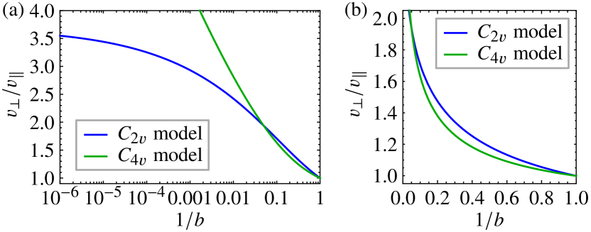
Figure 3: Ratio of Fermi velocities $v_{\perp}/v_{\parallel}$ as function of RG scale $1/b$ for both models. We assume ultraviolet initial values of $v_{\parallel}(b=1)=v_{\perp}(b=1)=0.25$, and set $g^{2}/(v_{\parallel}v_{\perp})(b=1)$ to the value at the respective stable fixed point. (a) Semilogarithmic, (b) linear plots. Starting at a temperature scale representative of the ultraviolet initial parameters, one has to cool the system by 2 orders of magnitude to start observing the differences between both models.

$\epsilon$ expansion.

The presence of a unique upper critical spatial dimension of three allows an $\epsilon=3-d$ expansion, with $\epsilon=1$ corresponding to the physical case. Because of the lack of Lorentz and continuous spatial rotational symmetries in the low-energy models, it is useful to employ a regularization in the frequency only, which allows us to rescale the different momentum components independently, and evaluate the loop integrals analytically [22]. Two central properties of nematic quantum phase transitions in Dirac systems are revealed by the one-loop RG analysis: First, both models admit a stable fixed point featuring anisotropic power laws of the fermion and order parameter correlation functions. In the $C_{2v}$ model, both components of the Fermi velocity remain finite at the stable fixed point with $0<v_{\parallel}^{*}<v_{\perp}^{*}$. At the critical point, a unique timescale $\tau$ emerges for both fields $\Psi$ and $\phi$ [23, 24], which scales with the two characteristic length scales $\ell_{+}$ and $\ell_{-}$ as $\tau\sim\ell_{+}^{z_{+}}\sim\ell_{-}^{z_{-}}$, with associated dynamical critical exponents $z_{\pm}=[1-\frac{1}{2}\eta_{\phi}+\frac{1}{2}\eta_{\pm}]^{-1}$ as $(z_{+},z_{-})=(1+0.3695\epsilon,1+0.1086\epsilon)+\mathcal{O}(\epsilon^{2})$, reflecting the absence of Lorentz and rotational symmetries at criticality. By contrast, in the $C_{4v}$ model, the fixed point is characterized by a maximal velocity anisotropy with $(v_{\parallel}^{*},v_{\perp}^{*})=(0,1)$ in units of fixed boson velocities $c\equiv c_{+}=c_{-}=1$. This result is consistent with the large-$N$ RG analysis in fixed $d=2$ [16]. The fact that $v_{\parallel}^{*}$ vanishes leads to the interesting behavior that the fixed-point couplings $g^{2}_{*}$ and $\lambda_{*}$ are bound to vanish in this case as well. This happens in a way that the ratio $(g^{2}/v_{\parallel})_{*}$ remains finite, such that the boson anomalous dimensions become $\eta_{\phi}=\eta_{+}=\eta_{-}=\epsilon$. Importantly, as the fixed-point couplings $g^{2}_{*}$ and $\lambda^{*}$ vanish, we expect the one-loop result for the critical exponents to hold at all loop orders in the $C_{4v}$ model. For the correlation-length exponent, we find $1/\nu=2-\epsilon$. The remaining exponents can then be computed by assuming the usual hyperscaling relations [25]. The susceptibility exponent, for instance, becomes $\gamma=1$, independent of $\epsilon$. This result is again consistent with the large-$N$ calculation and has previously already been argued to hold exactly [16]. We note that the values of the exponents in the $C_{4v}$ model are independent of the number of spinor components, in contrast to the situation in the $C_{2v}$ model, as well as to the usual Gross-Neveu universality classes [7, 8, 9, 10, 21, 26]. The unique dynamical critical exponent in the $C_{4v}$ model becomes $z=1$. We emphasize, however, that the critical point still does not feature emergent Lorentz symmetry [27] due to the anisotropic fermion spectral function. The second important property revealed by the RG analysis is that the stable fixed points in both models are approached only extremely slowly as function of RG scale, Fig. 3. This is universally true for the $C_{4v}$ model, in which case $v_{\parallel}$ corresponds to a marginally irrelevant parameter, hence scaling only logarithmically to zero while other irrelevant operators rapidly die out. This defines a quasiuniversal flow [28, 29] in which only the velocity anisotropy and not the initial ultraviolet values of other parameters determine the slow drift of the exponents. The RG suggests that this regime emerges at scales $1/b\lesssim 0.05$ (see Ref. [22]), such that it will dominate numerical as well as experimental realizations of this critical phenomena. For a reasonable set of ultraviolet starting values and $\epsilon=1$, we find that the effective correlation-length exponent $1/\nu_{\text{eff}}$ (anomalous dimension $\eta_{\phi}^{\text{eff}}$) approaches one from above (below), with sizable deviations at intermediate RG scales, see Ref. [22] for details. Moreover, we also observe that the initial flows at high energy in the two models resemble each other, despite the fact that they substantially deviate from each other at low energy. This suggests that the flow is generically slow in the $C_{2v}$ model as well.

QMC setup.

For the numerical simulations, we used the ALF program package [30] that provides a general implementation of the finite-temperature auxiliary field QMC algorithm [31, 32, 33]. To formulate the path integral, we use a Trotter decomposition with time step $\Delta_{\tau}t=0.1$ and choose a basis where $\hat{s}_{\bm{R}}^{z}|s_{\bm{R}}\rangle=s_{\bm{R}}|s_{\bm{R}}\rangle$. The configuration space is that of a $(2+1)$-dimensional Ising model and we use a single-spin-flip update to sample it. As shown in the Supplemental Material [22] both models are negative-sign-problem free for all values of $N_{\sigma}$ [34]. For our simulations, we have used an inverse temperature $\beta=4L$ for $L\times L$ lattices, and have checked that this choice of $\beta$ reflects ground-state properties. For the results shown in the main text, we have fixed the parameters as $J=t=1$ and $N_{\sigma}=2$. In the $C_{2v}$ model, we choose $\xi=0.25$, as larger values of $\xi$ lead to spurious size effects that could falsely be interpreted as first-order transitions, see Ref. [21] and the Supplemental Material [22] for a detailed discussion. In the $C_{4v}$ model, we set $\xi=1$. As shown in the Supplemental Material [22], other values of $\xi$ and $N_{\sigma}$ do not alter the continuous nature of the transition.

QMC results.

We compute the spin structure factor, $S({\bf k})=\sum_{\bf R}e^{i{\bf k\cdot R}}\Braket{\hat{s}^{z}_{\bf 0}\hat{s}^{z}_{\bf R}}$, the spin susceptibility, $\chi({\bf k})=\sum_{\bf r}e^{i{\bf k\cdot R}}\int_{0}^{\beta}\!{\rm d}\tau\,\Braket{\hat{s}^{z}_{\bf R}(\tau)\hat{s}^{z}_{{\bf 0}}(0)}$ and moments of the total spin $\hat{s}^{z}=\sum_{\bf R}\hat{s}^{z}_{\bf R}$ to derive RG-invariant quantities such as the correlation ratio [35],

$$R_{O}=1-\frac{O(\bm{k}_{\text{min}})}{O(\bm{k}=\bm{0})}\quad\text{with}\quad O=S,\chi,$$ (6)

and the Binder ratio, $B=\left(3-\frac{\langle(\hat{s}^{z})^{4}\rangle}{\langle(\hat{s}^{z})^{2}\rangle^{2}}\right)/2$. Here, $\bm{k}_{\text{min}}$ corresponds to the longest wavelength on a given finite-size lattice. From the single-particle Green’s function, we can extract quantities such as the fermion dispersion relation and Fermi velocities.

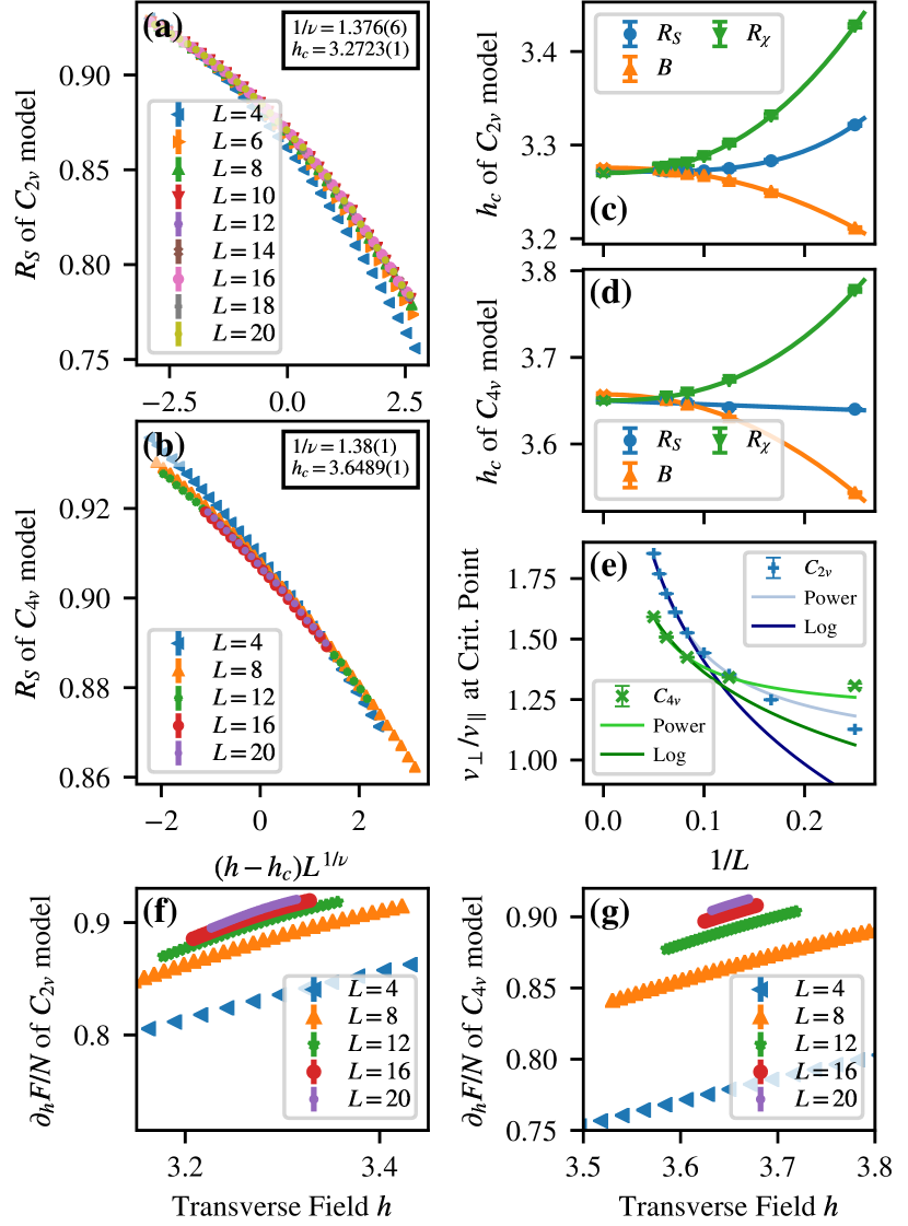
Figure 4: (a) $R_{S}$ as function of $(h-h_{\mathrm{c}})L^{1/\nu}$ for the $C_{2v}$ model, revealing data collapse for $L\gtrsim 12$, assuming $1/\nu=1.376$. (b) Same as (a), but for $C_{4v}$ model, assuming $1/\nu=1.38$. (c) Crossing points of different RG-invariant quantities as function of $1/L$ with $\Delta L=2$ in $C_{2v}$ model, indicating a unique critical point $h_{\mathrm{c}}=3.27$ for $L\to\infty$. (d) Same as (c), but for $C_{4v}$ model and $\Delta L=4$, extrapolating to $h_{\mathrm{c}}=3.65$ (e) Ratio of Fermi velocities $v_{\perp}/v_{\parallel}$ as function of $1/L$ at $h_{\mathrm{c}}$, revealing that the velocity anisotropy increases with increasing system size. The solid lines show power law fits for $L\geq 8$ and logarithmic fits for $L\geq 12$. (f),(g) Derivative of free energy as function of $h$, exhibiting no discontinuities.

At a quantum critical point, RG-invariant quantities follow the form $f[L^{z}/\beta,(h-h_{c})L^{1/\nu},L^{-\Delta z},L^{-\omega}]$ [22]. Here we have taken into account the possibility of two characteristic length scales: $\Delta z=1-z_{-}/z_{+}$. Since our temperature is representative of the ground state, we can neglect the dependence on $L^{z}/\beta$. Up to corrections to scaling, $\omega$, and the possibility of $z_{-}\neq z_{+}$, which would result in another correction to scaling term, the data for different lattice sizes cross at the critical field $h_{\mathrm{c}}$. Figs. 4(c,d) show the crossing points between $L$ and $L+\Delta L$ lattices, with $\Delta L=2$ $(4)$ for the $C_{2v}$ ($C_{4v}$) model. As apparent, we obtain consistent results for $h_{\mathrm{c}}$ when considering different RG-invariant quantities. We estimate the correlation-length exponents $1/\nu$ by data collapse for the two models in Figs. 4(a,b). Considering values of $L\geq L_{\text{min}}=12$ we obtain $1/\nu=1.376(6)$ [$1/\nu=1.38(1)$] for the $C_{2v}$ ($C_{4v}$) model. These values are in the ballpark of the $\epsilon$-expansion results in the quasiuniversal regime [22]. The data for various values of $L_{\text{min}}$ are given in the Supplemental Material [22], and stand in agreement with the above values. Although seemingly converged, the fact that the velocity anisotropy is expected to flow extremely slowly suggest that the exponents are subject to considerable size effects, see below. Figures 4(f,g) show the derivative of the free energy with respect to the tuning parameter, $\partial F/\partial h$, confirming the absence of any discontinuity at $h_{\mathrm{c}}$. The impact of critical fluctuations on the fermion spectrum is displayed in Figs. 2(b,c). In the disordered phase, Fig. 2(b), the dispersion relation exhibits rotational symmetry around the Dirac points. On the other hand, at criticality, Fig. 2(c), the dispersion relation suggests a velocity anisotropy, $v_{\parallel}<v_{\perp}$ at the Dirac point. Figure 4(e) demonstrates that this anisotropy grows as a function of system size, in qualitative agreement with the RG predictions. Although our system sizes are too small to detect convergence or divergence of the velocity ratio, we find it reassuring that its dependence on system size qualitatively resembles the scale dependence predicted from the integrated RG flow, cf. Fig. 4(e) with Fig. 3.

Summary.

Both the $\epsilon$-expansion analysis and the QMC simulations show that our two symmetry distinct models of Dirac fermions support continuous nematic transitions. In both cases, the key feature of the quantum critical point is a velocity anisotropy that is best seen in the QMC data of Fig. 2(c). For the $C_{4v}$ model, the $\epsilon$-expansion shows that it diverges logarithmically with system size, in agreement with previous large-$N$ results [16]. This law is supported by finite-size analysis based on QMC data up to linear system size $L=20$, which is close to the upper bound allowed by current computational approaches. Since the effective exponents flow with the velocity anisotropy, we foresee that lattice sizes beyond the reach of our numerical approach and experiments at ultralow temperatures will be required to obtain converged values. The QMC data captures a quasiuniversal regime [28, 29], in which irrelevant operators aside from the velocity anisotropy die out. In fact, the RG prediction for exponents in this intermediate-energy regime is roughly consistent with the finite-size QMC measurements, Fig. 13(c) of Ref. [22]. Furthermore, for a reasonable set of starting values, the integrated RG flows of the two models are initially very similar and deviate from each other only at very low energy scales. A similar behavior of the two models is also observed in the QMC data.

An advantage of our models is that the Dirac points are pinned by symmetry, such that QMC approaches that take momentum-space patches around these points into account [36] represent an attractive direction for future work. Our models equally allow for large-$N$ generalizations, such that QMC and analytical large-$N$ calculations can be compared as a function of increasing $N$. Finally, we can make contact to nematic transitions in $(2+1)$-dimensional Fermi liquids [12, 13], since our models do not suffer from the negative-sign problem under doping.

Acknowledgements.

This research has been funded by the Deutsche Forschungsgemeinschaft (DFG) through the Würzburg-Dresden Cluster of Excellence on Complexity and Topology in Quantum Matter ct.qmat – Project No. 390858490 (L. J., M. V., F. F. A.), the SFB 1170 on Topological and Correlated Electronics at Surfaces and Interfaces – Project No. 258499086 (J. S., F. F. A.), the SFB 1143 on Correlated Magnetism – Project No. 247310070 (L. J., M. V.), the Emmy Noether program – Project No. 411750675 (L. J.), the National Science and Engineering Council (NSERC) of Canada (I. F. H.), and Grant No. AS 120/14-1 (F. F. A.). Z. Y. M. acknowledges the Research Grants Council of Hong Kong China (Grants No. 17303019, No. 17301420, No. 17301721 and No. AoE/P-701/20) and the Strategic Priority Research Program of the Chinese Academy of Sciences (Grant No. XDB33000000), the K. C. Wong Education Foundation (Grant No. GJTD-2020-01) and the Seed Funding Quantum-Inspired explainable-AI at the HKU-TCL Joint Research Centre for Artificial Intelligence. We are grateful to the Gauss Centre for Supercomputing e.V. (www.gauss-centre.eu) for providing computing time on the GCS Supercomputer SUPERMUC-NG at Leibniz Supercomputing Centre (www.lrz.de).

Supplemental Material: Nematic quantum criticality in Dirac systems

I Absence of negative sign problem

Here we use the Majorana representation to demonstrate, using the results of Ref. [34], the absence of negative sign problem for all values of $N_{\sigma}$. Both models have $SU(N_{\sigma})$ symmetry. Since the Ising spins couple symmetrically to the fermion spins, $SU(N_{\sigma})$ symmetry is present for all Ising spin configurations. Thereby, the fermion determinant of the $SU(N_{\sigma})$ model corresponds to that of the $U(1)$ model ($N_{\sigma}=1$) elevated to the power $N_{\sigma}$. It hence suffices to demonstrate the absence of negative sign problem at $N_{\sigma}=1$. In this section, we will hence omit the spin index. Additionally we include a chemical potential term $\mathcal{H}_{\mu}$, to show that there is also no sign problem under doping for even values of $N_{\sigma}$.

I.1 The $C_{2v}$ model

Consider the canonical transformation,

$$\begin{pmatrix}\hat{a}_{\bm{k}}\\ \hat{b}_{\bm{k}}\end{pmatrix}\rightarrow\begin{pmatrix}1&0\\ 0&e^{-i3\pi/4}\end{pmatrix}\begin{pmatrix}\hat{a}_{\bm{k}-\Delta\bm{K}}\\ \hat{b}_{\bm{k}-\Delta\bm{K}}\end{pmatrix}$$ (7)

with

$$\hat{b}_{\bm{R}}=\frac{1}{\sqrt{N}}\sum_{\bm{k}\in BZ}e^{i\bm{k}\cdot\bm{R}}\hat{b}_{\bm{k}}$$ (8)

and $\Delta\bm{K}=\frac{1}{4}\left(\bm{b}_{-}-\bm{b}_{+}\right)$. Here , $\bm{e}_{i}\cdot\bm{b}_{j}=2\pi\delta_{i,j}$. This canonical transformation renders the Hamiltonian real: the $\pi$-flux, is realized by changing the sign of the intra unit-cell hopping with respect to the other hoppings. More precisely after the transformation, the Fermionic part of the Hamiltonian takes the form:

$$\mathcal{H}_{0}^{C_{2v}}=-t\sum_{\bm{R}}\hat{a}_{\bm{R}}^{\dagger}\Big{(}-\hat{b}_{\bm{R}}+\hat{b}_{\bm{R}+\bm{e}_{-}}+\hat{b}_{\bm{R}+\bm{e}_{-}-\bm{e}_{+}}s+\hat{b}_{\bm{R}-\bm{e}_{+}}\Big{)}+h.c.$$ (9a)

$$\mathcal{H}_{\text{Yuk}}^{C_{2v}}=-\xi\sum_{\bm{R}}s_{\bm{R}}\hat{a}^{\dagger}_{\bm{R}}\Big{(}-\hat{b}_{\bm{R}}-\hat{b}_{\bm{R}+\bm{e}_{-}}-\hat{b}_{\bm{R}+\bm{e}_{-}-\bm{e}_{+}}+\hat{b}_{\bm{R}-\bm{e}_{+}}\Big{)}+h.c.$$ (9b)

$$\mathcal{H}_{\mu}^{C_{2v}}=\mu\sum_{\bm{R}}\Big{(}\hat{a}^{\dagger}_{\bm{R}}\hat{a}_{\bm{R}}+\hat{b}^{\dagger}_{\bm{R}}\hat{b}_{\bm{R}}\Big{)}$$ (9c)

In the above, we have considered an arbitrary set of Ising spins $s_{\bm{R}}=\pm 1$.

Since equation (9) is real, the corresponding fermion determinant for $N_{\sigma}=1$ is also real and therefore positive for even $N_{\sigma}$.

For the sign to remain positive with odd $N_{\sigma}$, we have to dismiss $H_{\mu}$ and introduce Majorana fermions:

$$\hat{a}^{\dagger}_{\bm{R}} =\tfrac{1}{2}\left(\hat{\gamma}_{\bm{R},1}-i\hat{\bm{\gamma}}_{\bm{R},2}\right) \hat{b}^{\dagger}_{\bm{R}}=\tfrac{1}{2}\left(i\hat{\eta}_{\bm{R},1}+\hat{\eta}_{\bm{R},2}\right).$$ (10)

In the Majorana basis, the Fermionic part of the Hamiltonian reads:

$$\begin{split}&\mathcal{H}_{0}^{C_{2v}}=\frac{it}{2}\sum_{\bm{R}}\hat{\bm{\gamma}}^{\rm T}_{\bm{R}}\Big{(}-\hat{\bm{\eta}}_{\bm{R}}+\hat{\bm{\eta}}_{\bm{R}+\bm{e}_{-}}+\hat{\bm{\eta}}_{\bm{R}+\bm{e}_{-}-\bm{e}_{+}}+\hat{\bm{\eta}}_{\bm{R}-\bm{e}_{+}}\Big{)}\end{split}$$ (11a)

$$\begin{split}&\mathcal{H}_{\text{Yuk}}^{C_{2v}}=\frac{i\xi}{2}\sum_{\bm{R}}s_{\bm{R}}\hat{\bm{\gamma}}^{\rm T}_{\bm{R}}\Big{(}-\hat{\bm{\eta}}_{\bm{R},}-\hat{\bm{\eta}}_{\bm{R}+\bm{e}_{-}}-\hat{\bm{\eta}}_{\bm{R}+\bm{e}_{-}-\bm{e}_{+}}+\hat{\bm{\eta}}_{\bm{R}-\bm{e}_{+}}\Big{)}\end{split}$$ (11b)

In the above, $\bm{\hat{\gamma}}^{T}_{\bm{R}}=(\hat{\gamma}_{\bm{R},1},\hat{\gamma}_{\bm{R},2})$ and a similar form holds for $\bm{\hat{\eta}}_{\bm{R}}$. The fact that the Hamiltonian is diagonal in the Majorana index shows that it has a higher $O(2N_{\sigma})$ as opposed to the apparent $SU(N_{\sigma})$ one in the fermion representation. It also has for consequence that for the $N_{\sigma}=1$ case, the fermion determinant is nothing but the square of a Pfaffian that takes real values. Hence the negative sign problem is absent [37, 38]. We close this subsection by making contact with the work of Ref. [34]. Let $\bm{\mu}$ be a vector of Pauli matrices acting on the Majorana index. Adopting the notation of Ref. [34], we can define:

$$\hat{T}^{-}_{1}\alpha\bm{\hat{\gamma}}_{\bm{R}}\left(\hat{T}^{-}_{1}\right)^{-1}=\overline{\alpha}i\bm{\mu}_{y}\bm{\hat{\gamma}}_{\bm{R}}$$

$$\hat{T}^{-}_{1}\alpha\bm{\hat{\eta}}_{\bm{R}}\left(\hat{T}^{-}_{1}\right)^{-1}=-\overline{\alpha}i\bm{\mu}_{y}\bm{\hat{\eta}}_{\bm{R}}$$ (12)

and

$$\hat{T}^{+}_{2}\alpha\bm{\hat{\gamma}}_{\bm{R}}\left(\hat{T}^{+}_{2}\right)^{-1}=\overline{\alpha}\bm{\mu}_{x}\bm{\hat{\gamma}}_{\bm{R}}$$

$$\hat{T}^{+}_{2}\alpha\bm{\hat{\eta}}_{\bm{R}}\left(\hat{T}^{+}_{2}\right)^{-1}=-\overline{\alpha}\bm{\mu}_{x}\bm{\hat{\eta}}_{\bm{R}}.$$ (13)

Since $\left[\hat{T}^{+}_{2},\mathcal{H}^{C_{2v}}\right]=\left[\hat{T}^{-}_{1},\mathcal{H}^{C_{2v}}\right]=0$ and $\hat{T}^{-}_{1}$ and $\hat{T}^{+}_{2}$ anti-commute, our Hamiltonian belongs to the so-called Majorana class, and is hence free of the negative sign problem.

I.2 The $C_{4v}$ model

Consider the spinor $\hat{\bm{c}}^{\dagger}_{\bm{R}}=\left(\hat{a}^{\dagger}_{\bm{R}},\hat{b}^{\dagger}_{\bm{R}}\right)$. With this notation, the fermionic part of the $C_{4v}$ model takes the form:

$$\mathcal{H}_{0}^{C_{4v}} = -t\sum_{\bm{R}\in A,\delta=\pm}\left(\hat{\bm{c}}_{\bm{R}}^{\dagger}\,\bm{e}_{+}\cdot{\bm{\tau}}\,\hat{\bm{c}}_{\bm{R}+\delta\bm{e}_{x}}+\hat{\bm{c}}_{\bm{R}}^{\dagger}\,\bm{e}_{-}\cdot{\bm{\tau}}\,\hat{\bm{c}}_{\bm{R}+\delta\bm{e}_{y}}+h.c.\right)$$ (14a)

$$\mathcal{H}_{\text{Yuk}}^{C_{4v}} = \xi\sum_{\bm{R}}s_{\bm{R}}\hat{\bm{c}}^{\dagger}_{\bm{R}}\bm{e}_{y}\cdot\bm{\tau}\hat{\bm{c}}_{\bm{R}}$$ (14b)

$$\mathcal{H}_{\mu}^{C_{4v}} = \mu\sum_{\bm{R}}\hat{\bm{c}}^{\dagger}_{\bm{R}}\hat{\bm{c}}_{\bm{R}}$$ (14c)

In the above, $\bm{\tau}$ denotes a vector of Pauli matrices that act on the orbital space, $\bm{e}_{\pm}=\frac{1}{\sqrt{2}}\left(\bm{e}_{x}\pm\bm{e}_{y}\right)$, and $\bm{R}\in A$ denotes the sum of the A sub-lattice, $(-1)^{R_{x}+R_{y}}=1$. We have also considered an arbitrary set of Ising spins $s_{\bm{R}}=\pm 1$. Consider the relation,

$$U^{\dagger}(\bm{e},\theta)\bm{\tau}U(\bm{e},\theta)=R(\bm{e},\theta)\bm{\tau}$$ (15)

with $U(\bm{e},\theta)\bm{\tau}=e^{-i\theta\bm{e}\cdot\bm{\tau}/2}$ an SU(2) rotation of angle $\theta$ around axis $\bm{e}$ ($|\bm{e}|=1$ ) and $R(\bm{e},\theta)$ an SO(3) with same angle and axis. We can hence carry out a canonical transformation,

$$\hat{d}_{\bm{R}}=U\hat{c}_{\bm{R}},$$ (16)

that rotates $\bm{e}_{+}\rightarrow\bm{e}_{z}$, $\bm{e}_{-}\rightarrow\bm{e}_{x}$, and $\bm{e}_{y}\rightarrow-\frac{1}{\sqrt{2}}\left(\bm{e}_{x}-\bm{e}_{z}\right)$ by combing a $\pi/4$ rotation around the z-axis and subsequently a $\pi/2$ rotation around the x-axis. After this canonical transformation, the Hamiltonian is real, and takes the form:

$$\mathcal{H}_{0}^{C_{4v}} = -t\sum_{\bm{R}\in A,\delta=\pm}\left(\hat{\bm{d}}_{\bm{R}}^{\dagger}\,{\tau}_{z}\,\hat{\bm{d}}_{\bm{R}+\delta\bm{e}_{x}}+\hat{\bm{d}}_{\bm{R}}^{\dagger}\,{\tau}_{x}\,\hat{\bm{d}}_{\bm{R}+\delta\bm{e}_{y}}+h.c.\right)$$ (17a)

$$\mathcal{H}_{\text{Yuk}}^{C_{4v}} = -\frac{\xi}{\sqrt{2}}\sum_{\bm{R}}s_{\bm{R}}\hat{\bm{d}}^{\dagger}_{\bm{R}}\left(\tau_{x}-\tau_{z}\right)\hat{\bm{d}}_{\bm{R}}$$ (17b)

$$\mathcal{H}_{\mu}^{C_{4v}} = \mu\sum_{\bm{R}}\hat{\bm{d}}^{\dagger}_{\bm{R}}\hat{\bm{d}}_{\bm{R}}$$ (17c)

We can now express the model in terms of Majorana fermions and choose the following representation for $(-1)^{R_{x}+R_{y}}=1$,

$$\hat{\bm{d}}^{\dagger}_{\bm{R}}=\frac{1}{2}\left(\hat{\bm{\gamma}}_{\bm{R},1}-i\hat{\bm{\gamma}}_{\bm{R},2}\right)$$ (18)

and for $(-1)^{R_{x}+R_{y}}=-1$,

$$\hat{\bm{d}}^{\dagger}_{\bm{R}}=\frac{1}{2}\left(i\hat{\bm{\gamma}}_{\bm{R},1}+\hat{\bm{\gamma}}_{\bm{R},2}\right).$$ (19)

Let $\bm{\mu}$ be a vector of Pauli spin matrices that acts on the Majorana index. With this choice, the Hamiltonian then takes the form:

$$\mathcal{H}_{0}^{C_{4v}} = \frac{it}{2}\sum_{\bm{R}\in A,\delta=\pm}\left(\hat{\bm{\gamma}}_{\bm{R}}^{\rm T}\,{\bm{\tau}_{z}}\,\hat{\bm{\gamma}}_{\bm{R}+\delta\bm{e}_{x}}+\hat{\bm{\gamma}}_{\bm{R}}^{T}\,{\bm{\tau}}_{x}\,\hat{\bm{\gamma}}_{\bm{R}+\delta\bm{e}_{y}}\right)$$

$$\mathcal{H}_{\text{Yuk}}^{C_{4v}} = \frac{\xi}{4\sqrt{2}}\sum_{\bm{R}}s_{\bm{R}}\hat{\bm{\gamma}}^{\rm T}_{\bm{R}}\left(\bm{\tau}_{x}\bm{\mu}_{y}-\bm{\tau}_{z}\bm{\mu}_{y}\right)\hat{\bm{\gamma}}_{\bm{R}}$$ (20)

$$\mathcal{H}_{\mu}^{C_{4v}} = \mu\sum_{\bm{R}}\left(2-\hat{\bm{\gamma}}^{\rm T}_{\bm{R}}\mu_{y}\hat{\bm{\gamma}}_{\bm{R}}\right)$$ (21)

Using the notation of Ref. [34] we define:

$$\hat{T}^{-}_{1}\alpha\hat{\bm{\gamma}}_{\bm{R}}\left(\hat{T}^{-}_{1}\right)^{-1}=\overline{\alpha}i\bm{\tau}_{y}\bm{\mu}_{x}\hat{\bm{\gamma}}_{\bm{R}}$$ (22)

and

$$\hat{T}^{-}_{2}\alpha\hat{\bm{\gamma}}_{\bm{R}}\left(\hat{T}^{-}_{2}\right)^{-1}=\overline{\alpha}i\bm{\tau}_{y}\bm{\mu}_{z}\hat{\bm{\gamma}}_{\bm{R}}$$ (23)

that satisfy

$$\left[\mathcal{H}^{C_{4v}},\hat{T}^{-}_{1}\right]=\left[\mathcal{H}^{C_{4v}},\hat{T}^{-}_{2}\right]=0.$$ (24)

Both above symmetries square to (-1) and anti-commute with each other. This hence places us in the Kramers class, see Ref. [34, 39], and no negative sign problem occurs.

II Fourier transformed models

We define the Fourier transformation as:

$$\begin{pmatrix}\hat{a}_{\bm{R},\sigma}^{\dagger}\\ \hat{b}_{\bm{R},\sigma}^{\dagger}\end{pmatrix} =\frac{1}{\sqrt{N}}\sum_{\bm{k}}\mathrm{e}^{-i\bm{k}\bm{R}}\begin{pmatrix}\hat{a}_{\bm{k},\sigma}^{\dagger}\\ \hat{b}_{\bm{k},\sigma}^{\dagger}\end{pmatrix}$$ (25a)

$$s^{z}_{\bm{R}} =\frac{1}{N}\sum_{\bm{q}}s^{z}_{\bm{q}}\mathrm{e}^{i\bm{q}\bm{R}}$$ (25b)

with this definition, both models take the form

$$\mathcal{H} =-\sum_{\sigma=1}^{N_{\sigma}}\sum_{\bm{k}}\hat{a}_{\bm{k},\sigma}^{\dagger}\Bigg{(}\hat{b}_{\bm{k},\sigma}Z_{0}(\bm{k})+\frac{\xi}{N}\sum_{\bm{q}}\hat{b}_{\bm{k}-\bm{q},\sigma}s^{z}_{\bm{q}}Z_{\text{Yuk}}(\bm{k})\Bigg{)}+h.c.+H_{\text{Ising}}$$ (26a)

with

$$Z_{0}(\bm{k}) =\left\{\begin{array}[]{ll}2t\left(\mathrm{e}^{i\frac{\pi}{4}}\cos k_{x}+\mathrm{e}^{-i\frac{\pi}{4}}\cos k_{y}\right)\mathrm{e}^{-i\bm{k}_{y}}&C_{2v}\text{ model}\\ 2t\left(\mathrm{e}^{i\frac{\pi}{4}}\cos k_{x}+\mathrm{e}^{-i\frac{\pi}{4}}\cos k_{y}\right)&C_{4v}\text{ model}\end{array}\right.$$ (26d)

$$Z_{\text{Yuk}}(\bm{k}) =\left\{\begin{array}[]{ll}i2\left(-\mathrm{e}^{i\frac{\pi}{4}}\sin k_{x}+\mathrm{e}^{-i\frac{\pi}{4}}\sin k_{y}\right)\mathrm{e}^{-i\bm{k}_{y}}&C_{2v}\text{ model}\\ i&C_{4v}\text{ model.}\end{array}\right.$$ (26g)

III Symmetries

III.1 The $C_{2v}$ model

The First model has a $C_{2v}$ symmetry, consisting of two reflections: $T_{+}$ and $T_{-}$ on $\bm{e}_{\pm}=\bm{e}_{x}\pm\bm{e}_{y}$, the $\pi$ rotation needed by the point group can be obtained as $T_{\pi}=T_{+}\cdot T_{-}$. $T_{-}$ invariance hinges on the Z₂ Ising symmetry, $s^{z}\rightarrow-s^{z}$, and is therefore broken in the ordered phase.

The $C_{2v}$ symmetry pins the Dirac points (up to a gauge choice) to $(\pi/2,\pm\pi/2)$, while in the ordered phase, meandering parallel to $\bm{e}_{+}$ is possible.

To show this symmetry, we expand the momentum- and real-space vectors as: $\bm{k}=k_{+}\bm{e}_{+}+k_{-}\bm{e}_{-}$ and $\bm{R}=R_{+}\bm{e}_{+}+R_{-}\bm{e}_{-}$.

The first reflection $T_{+}$ reads:

$$\hat{T}_{+}^{-1}\begin{pmatrix}\hat{a}^{\dagger}_{\bm{k},\sigma}\\ \hat{b}^{\dagger}_{\bm{k},\sigma}\end{pmatrix}\hat{T}_{+} =\begin{pmatrix}\hat{b}^{\dagger}_{(k_{+},-k_{-}),\sigma}\phantom{\mathrm{e}^{-ik_{+}}}\\ \hat{a}^{\dagger}_{(k_{+},-k_{-}),\sigma}\mathrm{e}^{-ik_{+}}\end{pmatrix}$$ (27)

$$\hat{T}_{+}^{-1}s^{z}_{\bm{q}}\hat{T}_{+} =s^{z}_{(q_{+},-q_{-})}$$ (28)

Inserting the above in Eq. (26), we obtain:

$$\hat{T}_{+}^{-1}\mathcal{H}^{C_{2v}}\hat{T}_{+}=$$

$$=-\sum_{\bm{k}}\mathrm{e}^{ik_{+}}\hat{b}_{(k_{+},-k_{-}),\sigma}^{\dagger}\Bigg{(}\hat{a}_{(k_{+},-k_{-}),\sigma}Z_{0}^{C_{2v}}(\bm{k})+\xi\sum_{\bm{q}}\hat{a}_{(k_{+}-q_{+},-k_{-}+q_{-}),\sigma}\hat{s}^{z}_{(q_{+},-q_{-})}Z_{\text{Yuk}}^{C_{2v}}(\bm{k})\Bigg{)}+h.c.+H_{\text{Ising}}$$

$$=-\sum_{\bm{k}}\mathrm{e}^{-ik_{+}}\hat{a}_{(k_{+},k_{-}),\sigma}^{\dagger}\Bigg{(}\hat{b}_{(k_{+},k_{-}),\sigma}\bar{Z}_{0}^{C_{2v}}(k_{+},-k_{-})+\xi\sum_{\bm{q}}\hat{b}_{(k_{+}-q_{+},k_{-}-q_{-}),\sigma}\hat{s}^{z}_{(q_{+},q_{-})}\bar{Z}_{\text{Yuk}}^{C_{2v}}(k_{+},-k_{-})\Bigg{)}+h.c.+H_{\text{Ising}}$$

$$\qquad\left[\begin{array}[]{rl}\bar{Z}_{0}^{C_{2v}}(k_{+},-k_{-})&=Z_{0}^{C_{2v}}(\bm{k})\mathrm{e}^{ik_{+}}\\ \bar{Z}_{\text{Yuk}}^{C_{2v}}(k_{+},-k_{-})&=Z_{\text{Yuk}}^{C_{2v}}(\bm{k})\mathrm{e}^{ik_{+}}\end{array}\right]$$

$$=-\sum_{\bm{k}}\hat{a}_{(k_{+},k_{-}),\sigma}^{\dagger}\Bigg{(}\hat{b}_{(k_{+},k_{-}),\sigma}Z_{0}^{C_{2v}}(\bm{k})+\xi\sum_{\bm{q}}\hat{b}_{\bm{k}-\bm{q},\sigma}\hat{s}^{z}_{\bm{q}}Z_{\text{Yuk}}^{C_{2v}}(\bm{k})\Bigg{)}+h.c.+H_{\text{Ising}}$$

$$=\mathcal{H}^{C_{2v}}$$

In real space, $\hat{T}_{+}$ translates to:

$$\hat{T}_{+}^{-1}\begin{pmatrix}\hat{a}^{\dagger}_{\bm{R},\sigma}\\ \hat{b}^{\dagger}_{\bm{R},\sigma}\end{pmatrix}\hat{T}_{+} =\begin{pmatrix}\hat{b}^{\dagger}_{(R_{+},-R_{-}),\sigma}\\ \hat{a}^{\dagger}_{(R_{+}+1,-R_{-}),\sigma}\end{pmatrix}$$ (29)

$$\hat{T}_{+}^{-1}s^{z}_{\bm{R}}\hat{T}_{+} =s^{z}_{(R_{+},-R_{-})}$$ (30)

The second reflection $T_{-}$ can be expressed as:

$$\hat{T}_{-}^{-1}\begin{pmatrix}\hat{a}^{\dagger}_{\bm{k},\sigma}\\ \hat{b}^{\dagger}_{\bm{k},\sigma}\end{pmatrix}\hat{T}_{-} =\begin{pmatrix}\hat{b}^{\dagger}_{(-k_{+},k_{-}),\sigma}\phantom{\mathrm{e}^{ik_{-}}}\\ \hat{a}^{\dagger}_{(-k_{+},k_{-}),\sigma}\mathrm{e}^{ik_{-}}\end{pmatrix}$$ (31)

$$\hat{T}_{-}^{-1}s^{z}_{\bm{q}}\hat{T}_{-} =-s^{z}_{(-q_{+},q_{-})}$$ (32)

Inserting into Eq. (26), we obtain:

$$\hat{T}_{-}^{-1}\mathcal{H}^{C_{2v}}\hat{T}_{-}=$$

$$=-\sum_{\bm{k}}\mathrm{e}^{-ik_{-}}\hat{b}_{(-k_{+},k_{-}),\sigma}^{\dagger}\Bigg{(}\hat{a}_{(-k_{+},k_{-}),\sigma}Z_{0}(\bm{k})+\xi\sum_{\bm{q}}\hat{a}_{(-k_{+}+q_{+},k_{-}-q_{-}),\sigma}(-\hat{s}^{z}_{(-q_{+},q_{-})})Z_{\text{I}}(\bm{k})\Bigg{)}+h.c.+H_{\text{Ising}}$$

$$=-\sum_{\bm{k}}\mathrm{e}^{ik_{-}}\hat{a}_{(k_{+},k_{-}),\sigma}^{\dagger}\Bigg{(}\hat{b}_{(k_{+},k_{-}),\sigma}\bar{Z}_{0}(-k_{+},k_{-})+\xi\sum_{\bm{q}}\hat{b}_{(k_{+}-q_{+},k_{-}-q_{-}),\sigma}(-\hat{s}^{z}_{(q_{+},q_{-})})\bar{Z}_{\text{I}}(-k_{+},k_{-})\Bigg{)}+h.c.+H_{\text{Ising}}$$

$$\qquad\left[\begin{array}[]{rl}\bar{Z}_{0}(-k_{+},k_{-})&=Z_{0}^{C_{2v}}(\bm{k})\mathrm{e}^{-ik_{-}}\\ \bar{Z}_{\text{I}}(-k_{+},k_{-})&=-Z_{\text{Yuk}}^{C_{2v}}(\bm{k})\mathrm{e}^{-ik_{-}}\end{array}\right]$$

$$=-\sum_{\bm{k}}\hat{a}_{\bm{k},\sigma}^{\dagger}\Bigg{(}\hat{b}_{\bm{k},\sigma}Z_{0}^{C_{2v}}(\bm{k})+\xi\sum_{\bm{q}}\hat{b}_{\bm{k}-\bm{q}}\hat{s}^{z}_{\bm{q}}Z_{\text{Yuk}}^{C_{2v}}(\bm{k})\Bigg{)}+h.c.+H_{\text{Ising}}$$

$$=\mathcal{H}^{C_{2v}}$$

In real space, $\hat{T}_{-}$ translates to:

$$\hat{T}_{-}^{-1}\begin{pmatrix}\hat{a}^{\dagger}_{\bm{R},\sigma}\\ \hat{b}^{\dagger}_{\bm{R},\sigma}\end{pmatrix}\hat{T}_{-} =\begin{pmatrix}\hat{b}^{\dagger}_{(-R_{+},R_{-}),\sigma}\\ \hat{a}^{\dagger}_{(-R_{+},R_{-}-1),\sigma}\end{pmatrix}$$ (33)

$$\hat{T}_{-}^{-1}s^{z}_{\bm{R}}\hat{T}_{-} =s^{z}_{(-R_{+},R_{-})}$$ (34)

III.2 The $C_{4v}$ model

The Second model has a $C_{4V}$ symmetry, consisting of a rotation by $\tfrac{\pi}{2}$ and reflections on the x and y axis.

The corresponding operators are in momentum space:

$$\hat{T}_{\pi/2}^{-1}\begin{pmatrix}\hat{a}_{\bm{k},\sigma}^{{\dagger}}\\ \hat{b}_{\bm{k},\sigma}^{{\dagger}}\end{pmatrix}\hat{T}_{\pi/2} =\begin{pmatrix}\hat{b}_{(-k_{y},k_{x}),\sigma}^{{\dagger}}\\ \hat{a}_{(-k_{y},k_{x}),\sigma}^{{\dagger}}\end{pmatrix} \hat{T}_{x}^{-1}\begin{pmatrix}\hat{a}_{\bm{k},\sigma}^{{\dagger}}\\ \hat{b}_{\bm{k},\sigma}^{{\dagger}}\end{pmatrix}\hat{T}_{x} =\begin{pmatrix}\hat{a}_{(k_{x},-k_{y}),\sigma}^{{\dagger}}\\ \hat{b}_{(k_{x},-k_{y}),\sigma}^{{\dagger}}\end{pmatrix} \hat{T}_{y}^{-1}\begin{pmatrix}\hat{a}_{\bm{k},\sigma}^{{\dagger}}\\ \hat{b}_{\bm{k},\sigma}^{{\dagger}}\end{pmatrix}\hat{T}_{y} =\begin{pmatrix}\hat{a}_{(-k_{x},k_{y}),\sigma}^{{\dagger}}\\ \hat{b}_{(-k_{x},k_{y}),\sigma}^{{\dagger}}\end{pmatrix}$$ (35)

$$\hat{T}_{\pi/2}^{-1}\hat{s}^{z}_{\bm{q}}\hat{T}_{\pi/2} =-\hat{s}^{z}_{(-q_{y},q_{x})} \hat{T}_{x}^{-1}\hat{s}^{z}_{\bm{q}}\hat{T}_{x} =\hat{s}^{z}_{(q_{x},-q_{y})} \hat{T}_{y}^{-1}\hat{s}^{z}_{\bm{q}}\hat{T}_{y} =\hat{s}^{z}_{(-q_{x},q_{y})}$$ (36)

And in real space:

$$\hat{T}_{\pi/2}^{-1}\begin{pmatrix}\hat{a}_{\bm{R},\sigma}^{{\dagger}}\\ \hat{b}_{\bm{R},\sigma}^{{\dagger}}\end{pmatrix}\hat{T}_{\pi/2} =\begin{pmatrix}\hat{b}_{(-R_{y},R_{x}),\sigma}^{{\dagger}}\\ \hat{a}_{(-R_{y},R_{x}),\sigma}^{{\dagger}}\end{pmatrix} \hat{T}_{x}^{-1}\begin{pmatrix}\hat{a}_{\bm{R},\sigma}^{{\dagger}}\\ \hat{b}_{\bm{R},\sigma}^{{\dagger}}\end{pmatrix}\hat{T}_{x} =\begin{pmatrix}\hat{a}_{(R_{x},-R_{y}),\sigma}^{{\dagger}}\\ \hat{b}_{(R_{x},-R_{y}),\sigma}^{{\dagger}}\end{pmatrix} \hat{T}_{y}^{-1}\begin{pmatrix}\hat{a}_{\bm{R},\sigma}^{{\dagger}}\\ \hat{b}_{\bm{R},\sigma}^{{\dagger}}\end{pmatrix}\hat{T}_{y} =\begin{pmatrix}\hat{a}_{(-R_{x},R_{y}),\sigma}^{{\dagger}}\\ \hat{b}_{(-R_{x},R_{y}),\sigma}^{{\dagger}}\end{pmatrix}$$ (37)

$$\hat{T}_{\pi/2}^{-1}\hat{s}^{z}_{\bm{R}}\hat{T}_{\pi/2} =-\hat{s}^{z}_{(-R_{y},R_{x})} \hat{T}_{x}^{-1}\hat{s}^{z}_{\bm{R}}\hat{T}_{x} =\hat{s}^{z}_{(R_{x},-R_{y})} \hat{T}_{y}^{-1}\hat{s}^{z}_{\bm{R}}\hat{T}_{y} =\hat{s}^{z}_{(-R_{x},R_{y})}$$ (38)

In the Ising ordered phase, the Ising symmetry $\hat{s}^{z}_{\bm{R}}\rightarrow-\hat{s}^{z}_{\bm{R}}$ is broken, which reduces $\hat{T}_{\pi/2}$ to $\hat{T}_{\pi}$, such that the $C_{4v}$ symmetry is reduced to $C_{2v}$. This reduced symmetry allows the cones to meander.

Particle-hole symmetry:

$\hat{T}_{\text{ph}}$ This particle-hole symmetry implies that energy eigenstates satisfy $E(\bm{k})=-E(-\bm{k}+\bm{Q})$, $\bm{Q}=(\pi,\pi)$.

$$\hat{T}_{\text{ph}}^{-1}\alpha\begin{pmatrix}\hat{a}_{\bm{R},\sigma}^{\dagger}\\ \hat{b}_{\bm{R},\sigma}^{\dagger}\end{pmatrix}\hat{T}_{\text{ph}} =\overline{\alpha}(-1)^{R_{x}+R_{y}}\begin{pmatrix}\hat{a}_{\bm{R},\sigma}\\ \hat{b}_{\bm{R},\sigma}\end{pmatrix}$$ (39)

$$\hat{T}_{\text{ph}}^{-1}\alpha s^{z}_{\bm{R}}\hat{T}_{\text{ph}} =-\overline{\alpha}s^{z}_{\bm{R}}$$ (40)

$$\hat{T}_{\text{ph}}^{-1}\alpha\begin{pmatrix}\hat{a}^{\dagger}_{\bm{k},\sigma}\\ \hat{b}^{\dagger}_{\bm{k},\sigma}\end{pmatrix}\hat{T}_{\text{ph}} =\overline{\alpha}\begin{pmatrix}\hat{a}_{\bm{Q}-\bm{k},\sigma}\\ \hat{b}_{\bm{Q}-\bm{k},\sigma}\end{pmatrix}\quad\bm{Q}=\begin{pmatrix}\pi\\ \pi\end{pmatrix}$$ (41)

$$\hat{T}_{\text{ph}}^{-1}\alpha s^{z}_{\bm{q}}\hat{T}_{\text{ph}} =-\overline{\alpha}s^{z}_{-\bm{q}}$$ (42)

Inserting in Eq. (26), we obtain:

$$\hat{T}_{\text{ph}}^{-1}\mathcal{H}^{C_{4v}}\hat{T}_{\text{ph}} =-\sum_{\bm{k}}\hat{a}_{\bm{Q}-\bm{k}}\Bigg{(}\hat{b}^{\dagger}_{\bm{Q}-\bm{k}}\bar{Z}_{0}^{C_{4v}}(\bm{k})+\frac{\xi}{N}\sum_{\bm{q}}\hat{b}^{\dagger}_{\bm{Q}-\bm{k}+\bm{q}}\left(-s^{z}_{-\bm{q}}\right)\bar{Z}_{\text{Yuk}}^{C_{4v}}(\bm{k})\Bigg{)}+h.c.+H_{\text{Ising}}$$

$$=\phantom{-}\sum_{\bm{k}}\hat{a}^{\dagger}_{\bm{Q}-\bm{k}}\Bigg{(}\hat{b}_{\bm{Q}-\bm{k}}Z_{0}^{C_{4v}}(\bm{k})+\frac{\xi}{N}\sum_{\bm{q}}\hat{b}_{\bm{Q}-\bm{k}+\bm{q}}\left(-s^{z}_{-\bm{q}}\right)Z_{\text{Yuk}}^{C_{4v}}(\bm{k})\Bigg{)}+h.c.+H_{\text{Ising}}$$

$$=\phantom{-}\sum_{\bm{k}}\hat{a}^{\dagger}_{\bm{k}}\Bigg{(}\hat{b}_{\bm{k}}Z_{0}^{C_{4v}}(\bm{Q}-\bm{k})+\frac{\xi}{N}\sum_{\bm{q}}\hat{b}_{\bm{k}-\bm{q}}\left(-s^{z}_{\bm{q}}\right)Z_{\text{Yuk}}^{C_{4v}}(\bm{Q}-\bm{k})\Bigg{)}+h.c.+H_{\text{Ising}}$$

$$\qquad\left[\begin{array}[]{rl}Z_{0}^{C_{4v}}(\bm{Q}-\bm{k})&=-Z_{0}^{C_{4v}}(\bm{k})\\ Z_{\text{Yuk}}^{C_{4v}}(\bm{Q}-\bm{k})&=Z_{\text{Yuk}}^{C_{4v}}(\bm{k})\end{array}\right]$$

$$=-\sum_{\bm{k}}\hat{a}^{\dagger}_{\bm{k}}\Bigg{(}\hat{b}_{\bm{k}}Z_{0}^{C_{4v}}(\bm{k})+\frac{1}{N}\sum_{\bm{q}}\hat{b}_{\bm{k}-\bm{q}}\left(s^{z}_{\bm{q}}\right)Z_{\text{Yuk}}^{C_{4v}}(\bm{k})\Bigg{)}+h.c.+H_{\text{Ising}}$$

$$=\mathcal{H}^{C_{4v}}$$

As a result of this symmetry, the single particle spectral function satisfies $A(\bm{k},\omega)=A(-\bm{k}+\bm{Q},-\omega)$, with $\bm{Q}=(\pi,\pi)$.

IV Mean-field approximation

In the Mean-field approximation, we expand Eq. (26) around $\langle\hat{s}^{z}_{\bm{R}}\rangle\equiv\phi$. The resulting Mean-field Hamiltonian reads:

$$\mathcal{H}_{\text{MF}} =\sum_{\sigma=1}^{N_{\sigma}}\sum_{\bm{k}}\hat{K}_{\bm{k},\sigma}(\phi\xi)+\sum_{\bm{R}}\hat{I}_{\bm{R}}(\phi)$$ (43)

With:

$$\hat{K}_{\bm{k},\sigma}(\phi\xi) =-\hat{a}_{\bm{k},\sigma}^{\dagger}\hat{b}_{\bm{k},\sigma}Z(\bm{k},\phi\xi) Z(\bm{k},\phi\xi) =Z_{0}(\bm{k})+\phi\xi Z_{\text{Yuk}}(\bm{k}) \hat{I}_{\bm{R}}(\phi) =-4J\left(\phi\hat{s}^{z}_{\bm{R}}-\tfrac{1}{2}\phi^{2}\right)-h\hat{s}^{x}_{\bm{R}}$$

The fermionic dispersion is

$$\pm\left|Z(\bm{k},\phi\xi)\right|.$$ (44)

To determine the nature of the zero-temperature phase transition, we determine the order parameter $\phi$ for a given transverse field $h$ by minimizing the ground state energy $E_{0,\text{MF}}=\lim_{\beta\rightarrow\infty}E_{\text{MF}}=\lim_{\beta\rightarrow\infty}\Braket{\mathcal{H}_{\text{MF}}}_{\text{MF}}$.

$$E_{\text{MF}} =\Braket{\mathcal{H}_{\text{MF}}}_{\text{MF}}=\frac{{\rm Tr}\big{(}\exp(-\beta\mathcal{H}_{\text{MF}})\mathcal{H}_{\text{MF}}\big{)}}{{\rm Tr}\big{(}\exp(-\beta\mathcal{H}_{\text{MF}})\big{)}}$$

$$=N_{\sigma}\sum_{\bm{k}}|Z(\bm{k},\phi\xi)|\frac{1-\exp\left(\beta|Z(\bm{k},\phi\xi)|\right)}{1+\exp\left(\beta|Z(\bm{k},\phi\xi)|\right)}+L^{2}\left(2\phi^{2}-\sqrt{h^{2}+16\phi^{2}}\tanh\left(\beta\sqrt{h^{2}+16\phi^{2}}\right)\right)$$

$$\lim_{\beta\rightarrow\infty}\frac{E_{\text{MF}}}{L^{2}} =\underbrace{-\frac{N_{\sigma}}{L^{2}}\sum_{\bm{k}}|Z(\bm{k},\phi\xi)|}_{\epsilon_{\text{F}}(L,\phi\xi)}+\underbrace{\left(2\phi^{2}-\sqrt{h^{2}+16\phi^{2}}\right)}_{\epsilon_{\text{I}}(\phi,h)}$$ (45)

$$\partial_{\phi}\epsilon_{\text{F}}(L,\phi)=-\frac{N_{\sigma}}{L^{2}}\sum_{\bm{k}}\frac{1}{|Z(\bm{k},\phi)|}\Big{(}\Re\left(Z_{0}(\bm{k})\bar{Z}_{\text{Yuk}}(\bm{k})\right)+\phi|Z_{\text{Yuk}}(\bm{k})|^{2}\Big{)}$$ (46)

$$\partial^{2}_{\phi}\epsilon_{\text{F}}(L,\phi)=-\frac{N_{\sigma}}{L^{2}}\sum_{\bm{k}}\left(\frac{|Z_{\text{Yuk}}(\bm{k})|^{2}}{|Z(\bm{k},\phi)|}-\frac{\Re\left(Z_{0}(\bm{k})\bar{Z}_{\text{Yuk}}(\bm{k})\right)}{|Z(\bm{k},\phi)|^{3}}\Big{(}\Re\left(Z_{0}(\bm{k})\bar{Z}_{\text{Yuk}}(\bm{k})\right)+\phi|Z_{\text{Yuk}}(\bm{k})|\Big{)}\right)$$ (47)

Equation (45) separates into a fermionic and an Ising part, $\epsilon_{\text{F}}$ and $\epsilon_{\text{I}}$. While $\epsilon_{\text{I}}$ has a well-behaved, closed form, $\epsilon_{\text{F}}$ has some non-analytic points on finite lattices (see Fig. 6). Namely $\partial^{2}_{\phi}\epsilon_{\text{F}}$ diverges, if $Z(\bm{k},\phi\xi)$ vanishes.

This corresponds to a finite size artifact which can be qualitatively understood with the help of Fig. 5. Essentially, $\phi$, shifts the single particle energy and produces level crossing reminiscent of those produced when twisting boundary conditions [40, 41]. Fig.  5 shows the valence band of a one-dimensional Dirac cone on a lattice of size 5 $\bm{k}$ points at two different twists. As a function of the twist the $\bm{k}$-point will cross the Fermi surface and at this crossing point a singularity in the kinetic energy – corresponding to a level crossing – will appear. This is explicitly shown in Fig. 8. This observation means that the thermodynamic limit and the derivative $\partial_{\phi}$ do not commute: one should first take the thermodynamic limit prior to carrying out the derivative.

To avoid this artifact, we consider two different approaches:

1. Chose a weaker coupling $\xi$, such that the Dirac points do not cross the Fermi surface in proximity to the critical point. However, choosing a small $\xi$ may result in a slow flow from the 3d Ising fixed point of the unperturbed Ising model to nematic criticality.

2. Chose antiperiodic boundary conditions in space for the fermions, so to shift the $\bm{k}$-points away from the Fermi surface: Fig. 9. However, this choice results in large size effects presumably due to the boundary-condition induced finite size gap.

It turns out the first option is the best choice and that $\xi$ can be chosen large enough so as to minimize the aforementioned crossover effects.

The $C_{4v}$ model (Fig. 10) shows different behaviors between systems with linear size $L=2+4\mathbb{N}$ and $L=4\mathbb{N}$. At $L=4\mathbb{N}$ and periodic boundary conditions, the Dirac points in the disordered phase are located at $\bm{k}$-points resolved by the finite lattice. This is not the case at $L=2+4\mathbb{N}$ (cf. Fig. 11). As a result, the $L=4\mathbb{N}$ sizes have a smoothed out phase transition. Nevertheless, both $L=4\mathbb{N}$ and $L=2+4\mathbb{N}$ converge to the same result in the thermodynamic limit. The Monte-Carlo simulations also have odd-even effects, as elaborated in Section IX of this supplemental. It turns out that even system sizes produce nicer numerical results for the phase transition.

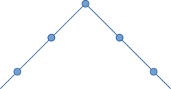
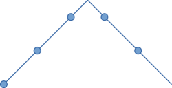
Figure 5: Sketch for understanding finite-size artifacts of Dirac systems as a function of $\bm{k}$-quantization. Shown is the valence band of a one-dimensional Dirac cone on a lattice of size $L=5$. We can see that the choice of the momenta quantization (i.e. boundary conditions) affects the energy. Left: Dirac cone belongs to the set of finite size $\bm{k}$-points. Right: Dirac cone is between two finite-size $\bm{k}$-points. Left has a higher ground state energy, and a level crossing occurs when a $\bm{k}$-point crosses the Fermi surface. In nematic transitions translation symmetry is not broken such that momenta is well defined and the $\bm{k}$ quantization for a given lattice size remains unchanged. However the position of the Dirac cone meanders. The energy level crossing that originates is reminiscent from that obtained when twisting boundary conditions [40, 41].

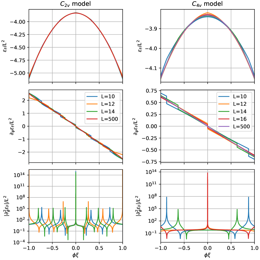
Figure 6: Fermionic part of Mean-field ground state energy.

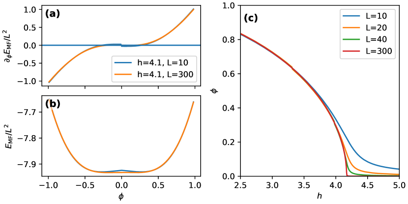
Figure 7: Mean-field results for the $C_{2v}$ model with $\xi=0.25$.

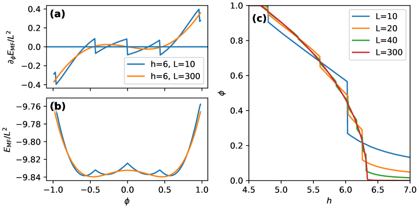
Figure 8: Mean-field results for the $C_{2v}$ model with coupling strength $\xi=0.75$.

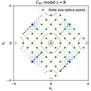
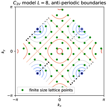
Figure 9: Brillouin zone of $C_{2v}$ model with $\bm{k}$ points of a $8*8$ lattice. Left: With periodic boundary conditions. Right: With antiperiodic boundary conditions for movement parallel to $(1,-1)$. Also sketched: Dispersion in disordered phase and trajectory of Dirac cones.

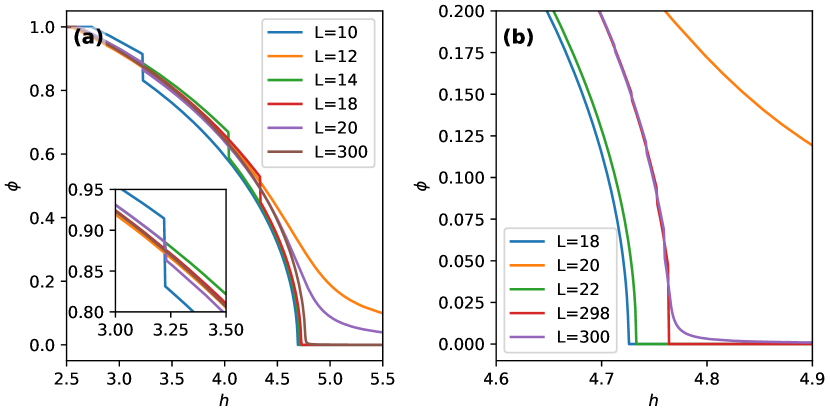
Figure 10: Mean-field results for the $C_{4v}$ model.

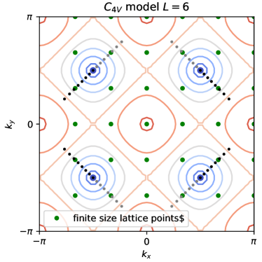
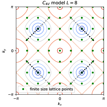
Figure 11: Brillouin zone of $C_{4v}$ model with $\bm{k}$ points of $6*6$ and $8*8$ lattice. Also sketched: Dispersion in disordered phase and trajectory of Dirac cones. Left: $6*6$ lattice, the Dirac cones in the disordered phase are each centered between four $\bm{k}$ points. Right: $8*8$ lattice, the Dirac cones in the disordered phase are directly resolved by the $\bm{k}$ points.

V Low energy models

We derive the low energy model from Eq. (26) by expansion in $\bm{k}$ around the nodal points $\bm{K}_{i}$ and for a scalar Ising field $\phi(\bm{q})$:

$$\mathcal{H} =-\sum_{\sigma=1}^{N_{\sigma}}\sum_{i}\int\!\text{d}\bm{\kappa}\;\hat{a}_{\bm{K}_{i}+\bm{\kappa},\sigma}^{\dagger}\Bigg{(}\hat{b}_{\bm{K}_{i}+\bm{\kappa},\sigma}Z_{0}(\bm{K}_{i}+\bm{\kappa})$$

$$+\frac{1}{2\pi}\int\!\text{d}\bm{q}\;\hat{b}_{\bm{K}_{i}+\bm{\kappa}-\bm{q},\sigma}\phi({\bm{q}})Z_{\text{Yuk}}(\bm{K}_{i}+\bm{\kappa})\Bigg{)}+h.c.+H_{\text{Ising}}\{\phi\}$$ (48)

In leading order in $\bm{\kappa}$ we obtain:

$$\mathcal{H} =-\sum_{\sigma=1}^{N_{\sigma}}\sum_{i}\int\!\text{d}\bm{\kappa}\;\hat{a}_{\bm{K}_{i}+\bm{\kappa},\sigma}^{\dagger}\Bigg{(}\hat{b}_{\bm{K}_{i}+\bm{\kappa},\sigma}\bm{\kappa}\nabla Z_{0}(\bm{K}_{i})$$

$$+\frac{1}{2\pi}\int\!\text{d}\bm{q}\;\hat{b}_{\bm{K}_{i}+\bm{\kappa}-\bm{q},\sigma}\phi({\bm{q}})Z_{\text{Yuk}}(\bm{K}_{i})\Bigg{)}+h.c.+H_{\text{Ising}}\{\phi\}.$$ (49)

Introducing the Fourier transformations:

$$\begin{pmatrix}\hat{a}^{i}_{\sigma}(\bm{r})\\ \hat{b}^{i}_{\sigma}(\bm{r})\end{pmatrix} =\frac{1}{2\pi}\int\!\text{d}\bm{\kappa}\;\mathrm{e}^{i\bm{\kappa}\bm{r}}\begin{pmatrix}\hat{a}_{\bm{K}_{i}+\bm{\kappa},\sigma}\\ \hat{b}_{\bm{K}_{i}+\bm{\kappa},\sigma}\end{pmatrix}$$

$$\phi(\bm{r}) =\frac{1}{2\pi}\int\!\text{d}\bm{\kappa}\;\mathrm{e}^{i\bm{q}\bm{r}}\phi(\bm{q}).$$

and defining:

$$\bm{v}_{i} \equiv\nabla Z_{0}(\bm{K}_{i}) I_{i} \equiv Z_{\text{Yuk}}(\bm{K}_{i})$$

The Hamiltonian takes the form:

$$\mathcal{H} =-\sum_{\sigma=1}^{N_{\sigma}}\sum_{i}\int\!\text{d}\bm{r}\;{\hat{a}^{i}_{\sigma}}{}(\bm{r})^{\dagger}\Big{(}i\bm{v}_{i}\cdot\nabla_{\bm{r}}+\phi(\bm{r})I_{i}\Big{)}\hat{b}^{i}_{\sigma}(\bm{r})+h.c.+H_{\text{Ising}}\{\phi\}$$ (50)

V.1 The $C_{2v}$ model

The $C_{2v}$ model has the nodal points $\bm{K}_{\pm}=\begin{pmatrix}\pi/2\\ \pm\pi/2\end{pmatrix}$. By defining the four-component Dirac spinor

$$\Psi_{\sigma}(\bm{r}) =\begin{pmatrix}\hat{a}^{+}_{\sigma}(\bm{r})&\hat{b}^{+}_{\sigma}(\bm{r})&\hat{a}^{-}_{\sigma}(\bm{r})&\hat{b}^{-}_{\sigma}(\bm{r})\end{pmatrix}^{\rm T}$$

and

$$\tau_{1} =\begin{pmatrix}0&1\\ 1&0\end{pmatrix} \tau_{2} =\begin{pmatrix}0&-i\\ i&0\end{pmatrix} \tau_{3} =\begin{pmatrix}1&0\\ 0&-1\end{pmatrix}.$$

Eq. (50) can be written as

$$\mathcal{H}^{C_{2v}} =\sum_{\sigma=1}^{N_{\sigma}}\int\!\text{d}\bm{r}\;\Psi_{\sigma}^{\dagger}(\bm{r})\Bigg{[}2it\begin{pmatrix}\tau_{2}&0\\ 0&-\tau_{1}\end{pmatrix}\partial_{r_{+}}+2it\begin{pmatrix}\tau_{1}&0\\ 0&-\tau_{2}\end{pmatrix}\partial_{r_{-}}+2\sqrt{2}\xi\phi(\bm{r})\begin{pmatrix}-\tau_{2}&0\\ 0&-\tau_{1}\end{pmatrix}\Bigg{]}\Psi_{\sigma}(\bm{r})+H_{\text{Ising}}\{\phi\}.$$

Introducing the gamma matrices

$$\gamma_{0} =\begin{pmatrix}-\tau_{3}&0\\ 0&-\tau_{3}\end{pmatrix} \gamma_{1} =\begin{pmatrix}\tau_{1}&0\\ 0&\tau_{2}\end{pmatrix} \gamma_{2} =\begin{pmatrix}-\tau_{2}&0\\ 0&-\tau_{1}\end{pmatrix} \{\gamma_{\alpha},\gamma_{\beta}\} =2\delta_{\alpha\beta},$$

we can write the action in the form

$$S^{C_{2v}}= \int\!\text{d}^{D}x\,\sum_{\sigma=1}^{N_{\sigma}}\Big{[}\Psi_{\sigma}^{\dagger}(x)\big{[}\openone\partial_{\tau}+v\gamma_{0}\gamma_{1}\partial_{+}+v\gamma_{0}\gamma_{2}\partial_{-}+g\phi(x)\gamma_{2}\big{]}\Psi_{\sigma}(x)\Big{]}+S_{\text{Ising}}(\{\phi\})$$ (51)

V.2 The $C_{4v}$ model

The $C_{4v}$ model has the nodal points $\bm{K}_{+\pm}=\begin{pmatrix}\pi/2\\ \pm\pi/2\end{pmatrix}$ and $\bm{K}_{-\pm}=-\bm{K}_{\pm}$. By defining the eight-component Dirac spinor

$$\Psi_{\sigma}(\bm{r}) =\begin{pmatrix}\hat{a}^{++}_{\sigma}(\bm{r})&\hat{b}^{++}_{\sigma}(\bm{r})&\hat{a}^{-+}_{\sigma}(\bm{r})&\hat{b}^{-+}_{\sigma}(\bm{r})&\hat{a}^{+-}_{\sigma}(\bm{r})&\hat{b}^{+-}_{\sigma}(\bm{r})&\hat{a}^{--}_{\sigma}(\bm{r})&\hat{b}^{--}_{\sigma}(\bm{r})\end{pmatrix}^{\rm T}$$

Eq. (50) can be written as

$$\mathcal{H}^{C_{4v}} =\sum_{\sigma=1}^{N_{\sigma}}\int\!\text{d}\bm{r}\;\Psi_{\sigma}^{\dagger}(\bm{r})\Bigg{[}$$

$$2it\Bigg{(}\begin{pmatrix}\tau_{1}&0\\ 0&-\tau_{1}\end{pmatrix}\oplus\begin{pmatrix}-\tau_{2}&0\\ 0&\tau_{2}\end{pmatrix}\Bigg{)}\partial_{r_{+}}+2it\Bigg{(}\begin{pmatrix}-\tau_{2}&0\\ 0&\tau_{2}\end{pmatrix}\oplus\begin{pmatrix}\tau_{1}&0\\ 0&-\tau_{1}\end{pmatrix}\Bigg{)}\partial_{r_{-}}+2\sqrt{2}\xi\phi(\bm{r})\Bigg{(}\begin{pmatrix}\tau_{2}&0\\ 0&\tau_{2}\end{pmatrix}\oplus\begin{pmatrix}\tau_{2}&0\\ 0&\tau_{2}\end{pmatrix}\Bigg{)}$$

$$\qquad\Bigg{]}\Psi_{\sigma}(\bm{r})+H_{\text{Ising}}\{\phi\}$$

Introducing the gamma matrices

$$\tilde{\gamma}_{0} =\begin{pmatrix}\tau_{3}&0\\ 0&-\tau_{3}\end{pmatrix} \tilde{\gamma}_{1} =\begin{pmatrix}\tau_{1}&0\\ 0&\tau_{1}\end{pmatrix} \tilde{\gamma}_{2} =\begin{pmatrix}\tau_{2}&0\\ 0&\tau_{2}\end{pmatrix} \{\tilde{\gamma}_{\alpha},\tilde{\gamma}_{\beta}\} =2\delta_{\alpha\beta}$$

We can write the action in the compact form

$$S^{C_{4v}}= \int\!\text{d}^{D}x\,\sum_{\sigma=1}^{N_{\sigma}}\Psi_{\sigma}^{\dagger}(x)\Big{[}\openone\partial_{\tau}+v\left(\tilde{\gamma}_{0}\tilde{\gamma}_{1}\oplus\tilde{\gamma}_{0}\tilde{\gamma}_{2}\right)\partial_{+}+v\left(\tilde{\gamma}_{0}\tilde{\gamma}_{2}\oplus\tilde{\gamma}_{0}\tilde{\gamma}_{1}\right)\partial_{-}+g\phi(x)\left(\tilde{\gamma}_{2}\oplus\tilde{\gamma}_{2}\right)\Big{]}\Psi_{\sigma}(x)+S_{\text{Ising}}(\{\phi\})$$ (52)

VI Renormalization group flow

In this section, we present details of the renormalization group (RG) analysis of the continuum field theories. Due to the lack of Lorentz and continuous spatial rotational symmetries in the low-energy models, the Fermi and bosonic velocities, as well as their anisotropies, will in general receive different loop corrections. In order to appropriately take this multiple dynamics [23, 24] into account, it is useful to employ a regularization in the frequency only, which preserves the property that the different momentum components can be rescaled independently. This allows us to keep the boson velocities $c\equiv c_{+}=c_{-}$ fixed, i.e., we measure the Fermi velocities in units of $c=1$. Integrating over the “frequency shell” $\Lambda/b\leq|\omega|\leq\Lambda$ with $b>1$ and all momenta causes the velocities and couplings to flow at criticality $r=0$ as

$$\frac{\mathrm{d}v_{\parallel}}{\mathrm{d}\ln b} =\frac{1}{2}(\eta_{\phi}-\eta_{+}-2\eta_{\psi})v_{\parallel}-F(v_{\parallel},v_{\perp})g^{2},$$ (53)

$$\frac{\mathrm{d}v_{\perp}}{\mathrm{d}\ln b} =\frac{1}{2}(\eta_{\phi}-\eta_{-}-2\eta_{\psi})v_{\perp}+F(v_{\perp},v_{\parallel})g^{2},$$ (54)

$$\frac{\mathrm{d}g^{2}}{\mathrm{d}\ln b} =\left(\epsilon-\frac{\eta_{+}+\eta_{-}}{2}-2\eta_{\psi}\right)g^{2}-2G(v_{\parallel},v_{\perp})g^{4},$$ (55)

$$\frac{\mathrm{d}\lambda}{\mathrm{d}\ln b} =\left(\epsilon-\frac{\eta_{+}+\eta_{-}}{2}-\eta_{\phi}\right)\lambda-18\lambda^{2}+\frac{N^{\prime}g^{4}}{16v_{\parallel}v_{\perp}},$$ (56)

with the anomalous dimensions $\eta_{\psi}=g^{2}H(v_{\parallel},v_{\perp})$, $\eta_{\phi}=N^{\prime}g^{2}/(12v_{\parallel}v_{\perp})$, and $\eta_{\pm}=a_{\pm}N^{\prime}g^{2}v_{\perp}/(12v_{\parallel})$, to the one-loop order. Here, the angular integrals are performed in $d=2$, while the dimensions of the couplings are counted in general $d$ [15, 42]. At the present order, the flows of the two models differ only in the definition of the coefficients $a_{\pm}$, with $a_{+}=0$, $a_{-}=2$ ($a_{+}=a_{-}=1$) in the $C_{2v}$ ($C_{4v}$) model, and the number of spinor components $N^{\prime}=4N_{\sigma}$ ($N^{\prime}=8N_{\sigma}$). Our regularization scheme allows the evaluation of the one-loop integrals in closed form, leading to the functions

$$F(v_{1},v_{2}) =\frac{1}{\pi}\int_{-\infty}^{\infty}\int_{-\infty}^{\infty}\frac{v_{1}q_{1}^{2}\mathrm{d}q_{1}\mathrm{d}q_{2}}{\left(1+q_{1}^{2}+q_{2}^{2}\right)^{2}\left(1+v_{1}^{2}q_{1}^{2}+v_{2}^{2}q_{2}^{2}\right)}$$

$$=\frac{v_{1}\left[v_{1}\left(v_{2}^{2}-1\right)\sqrt{\frac{1-v_{1}^{2}}{v_{2}^{2}-1}}+(v_{1}+v_{2})\sin^{-1}\left({v_{1}}{\sqrt{\frac{v_{2}^{2}-1}{v_{2}^{2}-v_{1}^{2}}}}\right)-(v_{1}+v_{2})\csc^{-1}\left(\sqrt{\frac{v_{2}^{2}-v_{1}^{2}}{v_{2}^{2}-1}}\right)\right]}{\left(v_{1}^{2}-1\right)\left(v_{2}^{2}-1\right)(v_{1}+v_{2})\sqrt{\frac{1-v_{1}^{2}}{v_{2}^{2}-1}}}\,,$$ (57)

$$G(v_{1},v_{2}) =\frac{1}{2\pi}\int_{-\infty}^{\infty}\int_{-\infty}^{\infty}\frac{1-v_{1}^{2}q_{1}^{2}+v_{2}^{2}q_{2}^{2}}{\left(1+q_{1}^{2}+q_{2}^{2}\right)\left(1+v_{1}^{2}q_{1}^{2}+v_{2}^{2}q_{2}^{2}\right)^{2}}\mathrm{d}q_{1}\mathrm{d}q_{2}$$

$$=\frac{\left(v_{2}^{2}-1\right)(v_{1}v_{2}-1)\sqrt{\frac{1-v_{1}^{2}}{v_{2}^{2}-1}}+\left(v_{1}^{2}+v_{2}^{2}-2\right)\csc^{-1}\left(\frac{1}{v_{1}}\sqrt{\frac{v_{2}^{2}-v_{1}^{2}}{v_{2}^{2}-1}}\right)-\left(v_{1}^{2}+v_{2}^{2}-2\right)\csc^{-1}\left(\sqrt{\frac{v_{2}^{2}-v_{1}^{2}}{v_{2}^{2}-1}}\right)}{2\left(v_{1}^{2}-1\right)\left(v_{2}^{2}-1\right)^{2}\sqrt{\frac{1-v_{1}^{2}}{v_{2}^{2}-1}}}$$

$$\quad+\frac{v_{1}\left[\left(v_{2}^{2}-1\right)\sqrt{\frac{1-v_{1}^{2}}{v_{2}^{2}-1}}-v_{1}(v_{1}+v_{2})\sin^{-1}\left({\sqrt{\frac{v_{2}^{2}-1}{v_{2}^{2}-v_{1}^{2}}}}\right)+v_{1}(v_{1}+v_{2})\csc^{-1}\left(\frac{1}{v_{1}}\sqrt{\frac{v_{2}^{2}-v_{1}^{2}}{v_{2}^{2}-1}}\right)\right]}{2\left(v_{1}^{2}-1\right)\left(v_{2}^{2}-1\right)(v_{1}+v_{2})\sqrt{\frac{1-v_{1}^{2}}{v_{2}^{2}-1}}}$$

$$\quad+\frac{v_{2}^{4}(v_{1}+v_{2})\sin^{-1}\left({\sqrt{\frac{v_{2}^{2}-1}{v_{2}^{2}-v_{1}^{2}}}}\right)}{2v_{2}^{2}\left(v_{2}^{2}-1\right)^{2}(v_{1}+v_{2})\sqrt{\frac{1-v_{1}^{2}}{v_{2}^{2}-1}}}+\frac{\left(v_{1}^{3}+v_{1}^{2}v_{2}+v_{1}v_{2}^{2}+v_{2}^{3}\right)\sin^{-1}\left({v_{1}}{\sqrt{\frac{v_{2}^{2}-1}{v_{2}^{2}-v_{1}^{2}}}}\right)-2\left(v_{1}^{2}-1\right)v_{2}^{3}\sqrt{\frac{1-v_{1}^{2}}{v_{2}^{2}-1}}}{4\left(v_{1}^{2}-1\right)v_{2}^{2}\left(v_{2}^{2}-1\right)(v_{1}+v_{2})\sqrt{\frac{1-v_{1}^{2}}{v_{2}^{2}-1}}}$$

$$\quad-\frac{\left(v_{2}^{2}+1\right)\left[v_{1}^{3}\left(2v_{2}^{2}-1\right)+v_{1}^{2}v_{2}\left(2v_{2}^{2}-1\right)-v_{1}v_{2}^{2}-v_{2}^{3}\right]\csc^{-1}\left(\frac{1}{v_{1}}\sqrt{\frac{v_{2}^{2}-v_{1}^{2}}{v_{2}^{2}-1}}\right)}{4\left(v_{1}^{2}-1\right)v_{2}^{2}\left(v_{2}^{2}-1\right)^{2}(v_{1}+v_{2})\sqrt{\frac{1-v_{1}^{2}}{v_{2}^{2}-1}}}\,,$$

$$H(v_{1},v_{2}) =\frac{1}{\pi}\int_{-\infty}^{\infty}\int_{-\infty}^{\infty}\frac{\mathrm{d}q_{1}\mathrm{d}q_{2}}{\left(1+q_{1}^{2}+q_{2}^{2}\right)^{2}\left(1+v_{1}^{2}q_{1}^{2}+v_{2}^{2}q_{2}^{2}\right)}$$

$$=\frac{\left(v_{1}^{2}+v_{2}^{2}-2v_{1}^{2}v_{2}^{2}\right)\left[\csc^{-1}\left(\sqrt{\frac{v_{2}^{2}-v_{1}^{2}}{v_{2}^{2}-1}}\right)-\csc^{-1}\left(\frac{1}{v_{1}}\sqrt{\frac{v_{2}^{2}-v_{1}^{2}}{v_{2}^{2}-1}}\right)\right]}{\left(v_{1}^{2}-1\right)\left(v_{2}^{2}-1\right)^{2}\sqrt{\frac{1-v_{1}^{2}}{v_{2}^{2}-1}}}-\frac{(v_{1}v_{2}-1)\sqrt{\frac{1-v_{1}^{2}}{v_{2}^{2}-1}}}{\left(v_{1}^{2}-1\right)\left(v_{2}^{2}-1\right)\sqrt{\frac{1-v_{1}^{2}}{v_{2}^{2}-1}}}\,.$$ (58)

The above one-loop flow equations admit a nontrivial fixed point that is characterized by anisotropic Fermi velocities $v_{\parallel}^{*}=0$ and $v_{\perp}^{*}=1/\sqrt{a_{-}}>0$, and vanishing $g^{2}_{*}$ and $\lambda^{*}$, but finite ratio $(g^{2}/v_{\parallel})_{*}=12\sqrt{a_{-}}\epsilon/N^{\prime}+\mathcal{O}(\epsilon^{2})$. Perturbations of the couplings $g^{2}$ and $\lambda$ and the Fermi velocity $v_{\perp}$ away from this fixed point turn out be irrelevant; however, the flow of $v_{\parallel}$ near the fixed point is

$$\left.\frac{\mathrm{d}v_{\parallel}}{\mathrm{d}\ln b}\right|_{g^{2}_{*},v_{\perp}^{*}} =\frac{\epsilon}{2}(1-a_{+})v_{\parallel}-\frac{20\epsilon}{N^{\prime}}v_{\parallel}^{2}+\mathcal{O}(v_{\parallel}^{3}).$$ (59)

Hence, in the $C_{4v}$ model with $a_{+}=a_{-}=1$, $v_{\parallel}$ is marginally irrelevant, rendering the fixed point stable. The fixed point represents a quantum critical point with maximally anisotropic Fermi velocities $(v_{\parallel}^{*},v_{\perp}^{*})=(0,1)$ and boson anomalous dimensions, describing the temporal and spatial decays of the order-parameter correlations, as $\eta_{\phi}=\epsilon$ and $\eta_{+}=\eta_{-}=\epsilon$, respectively. The fermion anomalous dimension becomes $\eta_{\psi}=0$. In the vicinity of this fixed point, the flow of $v_{\parallel}$ can be integrated out analytically, reading

$$v_{\parallel}(b)\simeq\frac{N^{\prime}}{20\epsilon\ln b},$$ (60)

where we have assumed $b\gg 1$ for simplicity. This demonstrates that the Fermi velocity flow in the vicinity of the $C_{4v}$ fixed point is logarithmically slow, reflecting the fact that $v_{\parallel}$ is marginally irrelevant at this fixed point. This indicates that exponentially large lattice sizes are needed to ultimate reach the fixed point. By contrast, in the $C_{2v}$ model with $a_{+}=0$ and $a_{-}=2$, $v_{\parallel}$ is a relevant parameter near the maximal-anisotropy fixed point and flows to larger values. By numerically integrating out the flow, we find that the parameters $v_{\perp}$, $v_{\parallel}$, and $g^{2}$ flow to a new nontrivial stable fixed point at which the boson anomalous dimensions satisfy a sum rule, $\eta_{+}+\eta_{-}+2\eta_{\phi}=2\epsilon$ with $0=\eta_{+}<\eta_{-},\eta_{\phi}<\epsilon$. The fixed point is located at $(v_{\parallel}^{*},v_{\perp}^{*})=(0.1611,0.5942)$ and $(g^{2}_{*},\lambda^{*})=(0.2123,0.1755)\epsilon+\mathcal{O}(\epsilon^{2})$ for $N^{\prime}=4N_{\sigma}=4$. We find the corresponding anomalous dimensions as $(\eta_{\phi},\eta_{+},\eta_{-},\eta_{\psi})=(0.7391,0,0.5219,0.1643)\epsilon+\mathcal{O}(\epsilon^{2})$, reflecting again the fact that the character of the stable fixed point in the $C_{2v}$ model is different from the one of the $C_{4v}$ model. The different behaviors of the Fermi velocities in the two models is illustrated in Fig. 12, which shows the renormalization group flow in the $v_{\parallel}$-$v_{\perp}$ plane. For visualization purposes, we have fixed the ratios $g^{2}/(v_{\perp}v_{\parallel})$ to their values at the respective stable fixed points in these plots. We have explicitly verified that $g^{2}/(v_{\perp}v_{\parallel})$ corresponds to an irrelevant parameter near these fixed points (marked as red dots in Fig. 12).

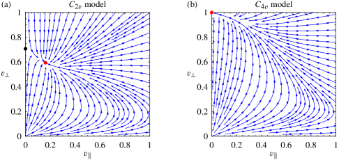
Figure 12: Renormalization group flow in the $v_{\parallel}$-$v_{\perp}$ plane for (a) the $C_{2v}$ model and (b) the $C_{4v}$ model. Arrows denote flow towards infrared. The fixed point at $(v_{\parallel}^{*},v_{\perp}^{*})=(0,1/\sqrt{a_{-}})$ and $(g^{2}/v_{\parallel})_{*}=12\sqrt{a_{-}}\epsilon/N^{\prime}$ is unstable in the $C_{2v}$ model [black dot in (a)], but stable in the $C_{4v}$ model [red dot in (b)]. In the $C_{2v}$ model, there is a nontrivial stable fixed point at $(v_{\parallel}^{*},v_{\perp}^{*})=(0.1611,0.5942)$, with $g^{2}_{*}=0.2123\epsilon$ for $N^{\prime}=4$ [red dot in (a)]. For visualization purposes, we have fixed the ratio $g^{2}/(v_{\perp}v_{\parallel})$ to its value at the respective stable fixed point (red dots) in these plots.

To make further contact with the QMC data displayed in Fig. 3(e) of the main text, we show in Fig. 13(a,b) the Fermi velocity ratio $v_{\perp}/v_{\parallel}$ as function of RG scale $1/b$ in the two models, assuming an isotropic ratio $v_{\perp}/v_{\parallel}=1$ at the ultraviolet scale $b=1$, for different initial values of the interaction parameter $g^{2}/(v_{\parallel}v_{\perp})$. We emphasize that a sizable deviation between the two models is observable only at very low energies $1/b\lesssim 0.01$, while the RG flows in the high-energy regime are very similar for the employed starting values. Identifying the RG energy scale $1/b$ roughly with the inverse lattice size $1/L$, this result explains why the lattice sizes available in our simulations are too small to detect a substantial difference in the finite-size scaling of $v_{\perp}/v_{\parallel}$. This also implies that the estimates for the critical exponent obtained from the finite-size analysis of the QMC data describes only an intermediate regime, in which the RG flow is not yet fully integrated out. Let us illustrate this point further for the case of the $C_{4v}$ model. In this case, we can define a scale-dependent effective correlation-length exponent by using the scaling relation

$$1/\nu_{\text{eff}}(b)=2-\eta_{\phi}^{\text{eff}}(b),$$ (61)

where $\eta_{\phi}^{\text{eff}}(b)=N^{\prime}g^{2}(b)/[12v_{\perp}(b)v_{\perp}(b)]$ is the effective boson anomalous dimension. This relation becomes exact in the vicinity of the $C_{4v}$ fixed point, for which $\lambda^{\ast}=0$. The effective correlation-length exponent $1/\nu_{\text{eff}}$ is plotted as function of the RG scale $1/b$ in Fig. 13(c) for different values of the initial interaction parameter $g^{2}/(v_{\parallel}v_{\perp})$. We note that the approach to $\nu_{\text{eff}}\to 1$ in the deep infrared is extremely slow, with sizable deviations from the fixed-point value at intermediate scales. Interestingly, while the behavior in the high-energy regime $1/b\gtrsim 0.05$ is nonuniversal and strongly depends on the particular starting values of the RG flow, a quasiuniversal regime emerges at intermediate energy $1/b\lesssim 0.05$, in which the exponents still drift, but have only a very weak dependence on the initial interaction parameters. This quasiuniversal behavior is a characteristic feature of systems with marginal or close-to-marginal operators [28, 29]. Here, it arises from the slow flow of the velocity anisotropy ratio $v_{\perp}/v_{\parallel}$, which implies that the effective exponents will become functions of $v_{\perp}/v_{\parallel}$ only, but not of the ultraviolet starting values of the interaction parameters. The quasiuniversality reflects the fact that there is only one slowly decaying perturbation to the fixed point (i.e., the leading irrelevant operator), whereas all other perturbations decay quickly, and hence have died out once $1/b\lesssim 0.05$. Importantly, the largest lattice sizes available in the QMC simulations appear to be just large enough to approach the quasiuniversal regime, if we again identify $1/b$ roughly with $1/L$. Reassuringly, for $L=20$, we therewith obtain the RG estimate $1/\nu_{\text{eff}}\simeq 1.20\dots 1.25$, which is in the same ballpark as the estimate from the finite-size scaling analysis of the QMC data discussed in the main text.

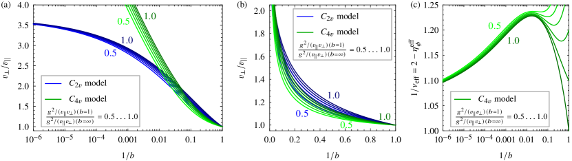
Figure 13: (a,b) Ratio of Fermi velocities $v_{\perp}/v_{\parallel}$ as function of RG scale $1/b$ in the $C_{2v}$ model (blue) and $C_{4v}$ model (green) for different starting values of the interaction parameter $g^{2}/(v_{\parallel}v_{\perp})$ at the ultraviolet scale $b=1$. Here, we have numerically integrated out the full RG flow in the $(v_{\parallel},v_{\perp},g^{2})$ parameter space, assuming initial velocities $v_{\parallel}(b=1)=v_{\perp}(b=1)=0.25$, and $g^{2}/(v_{\parallel}v_{\perp})(b=1)$ between 50% and 100% of the value at the respective stable fixed point. (a) Semilogarithmic plot, demonstrating the finite infrared anisotropy in the $C_{2v}$ model and the logarithmic divergence in the $C_{4v}$ model. (b) Same data as in (a), but using a linear plot, illustrating the similarity of the anisotropy flows in the two models on the high-energy scale, to be compared with the QMC data shown in Fig. 3(e) of the main text. (c) Effective correlation-length exponent $1/\nu_{\text{eff}}$ as function of RG scale $1/b$ in the $C_{4v}$ model in semilogarithmic plot, defined according to Eq. (61), illustrating the drifting of the exponents and the quasiuniversal behavior for $1/b\lesssim 0.05$. We have used the same ultraviolet starting values as in (a,b).

VII Observables

In this section, we define the observables used throughout this work to study the quantum phase transition. We have considered quantities based on bosonic and fermionic degrees of freedom.

VII.1 Bosonic degrees of freedom

The structure factor $S(\bm{k})$ and susceptibility $\chi(\bm{k})$ are defined as

$$S(\bm{k}) =\frac{1}{N^{2}}\sum_{\langle\bm{R},\bm{R}^{\prime}\rangle}\left(\langle s^{z}_{\bm{R}}s^{z}_{\bm{R}^{\prime}}\rangle-\langle s^{z}_{\bm{R}}\rangle\langle s^{z}_{\bm{R}^{\prime}}\rangle\right)e^{i\bm{k}(\bm{R}-\bm{R}^{\prime})},$$ (62)

and

$$\chi(\bm{k}) =\int\!\text{d}\tau\,\frac{1}{N^{2}}\sum_{\langle\bm{R},\bm{R}^{\prime}\rangle}\left(\Braket{s^{z}_{\bm{R}}(0)s^{z}_{\bm{R}^{\prime}}(\tau)}-\Braket{s^{z}_{\bm{R}}(0)}\Braket{s^{z}_{\bm{R}^{\prime}}(\tau)}\right)e^{i\bm{k}(\bm{R}-\bm{R}^{\prime})}.$$ (63)

Both $S(\bm{k}=0)$ and $\chi(\bm{k}=0)$ are suitable order parameters for the paramagnetic-ferromagnetic phase transision. Note that in the main text, these observables are defined without subtraction of the background $\langle s^{z}_{\bm{R}}\rangle\langle s^{z}_{\bm{R}^{\prime}}\rangle$, or $\Braket{s^{z}_{\bm{R}}(0)}\Braket{s^{z}_{\bm{R}^{\prime}}(\tau)}$. Generically, this is generally equivalent, since in a fully ergodic simulation the background vanishes by symmetry. In fact, the global move in the Monte Carlo sampling that flips all the spins has an acceptance of unity such that the background is identical to zero. In some case, it is convenient to omit this global move. In fact to image the meandering of the cones, Sec. VII.2.1, we omitted the global move so as to achieve $\braket{s^{z}}>0$ and observe the displaced Dirac cones.

By definition, renormalization group invariant quantities have vanishing scaling dimension. They can be derived from the correlation function and susceptibilities in terms of the correlation ratios $R_{S}$ and $R_{\chi}$

$$R_{O}=1-\frac{O(\bm{k}_{\text{min}})}{O(\bm{k}=\bm{0})}\quad\text{with}\quad O=S,\chi,$$ (64)

where $\bm{k}_{\text{min}}$ corresponds to the longest wave length on the considered lattice. Generally, one can chose instead of $\bm{k}_{\text{min}}$ any wave-vector that approaches $\bm{k}=0$ as $1/L$ to achieve the same asymptotic behavior. However, we have found that using $\bm{k}_{\text{min}}$ works best for us. Another RG-invariant quantity is the Binder ratio, $B$, defined as

$$B =\frac{1}{2}\left(3-\frac{\Braket{(s^{z})^{4}}}{\Braket{(s^{z})^{2}}^{2}}\right).$$ (65)

To provide further information on the nature of the transition, we have considered the derivative of the free energy,

$$\frac{1}{N}\frac{\partial F}{\partial h}=\Braket{\frac{1}{N}\sum_{\bm{R}}s^{x}_{\bm{R}}}\equiv X$$ (66)

VII.2 Fermionic degrees of freedom

The fermionic observables consist of the momentum-resolved single-particle gap $\Delta_{\text{sp}}(\bm{k})$ which we use to image the meandering of Dirac points. We furthermore use this quantity to determine the velocity anisotropy.

VII.2.1 Fermionic single-particle gap

To properly define $\Delta_{\text{sp}}(\bm{k})$, we first introduce an energy basis:

$$\mathcal{H}\Ket{\Psi^{N}_{n}(\bm{k})}=E^{N}_{n}(\bm{k})\Ket{\Psi^{N}_{n}(\bm{k})},$$ (67)

where $\Ket{\Psi^{N}_{n}(\bm{k})}$ are also eigenstates of particle number $\hat{N}$ and momentum $\hat{\bm{k}}$ operators:

$$\hat{N}\Ket{\Psi^{N}_{n}(\bm{k})} =N\Ket{\Psi^{N}_{n}(\bm{k})} \hat{\bm{k}}\Ket{\Psi^{N}_{n}(\bm{k})} =\bm{k}\Ket{\Psi^{N}_{n}(\bm{k})}$$ (68)

In this basis, the gap is:

$$\Delta_{\text{sp}}(\bm{k})=E_{0}^{N_{0}+1}(\bm{k})-E_{0}^{N_{0}},$$ (69)

where $N_{0}$ is the particle number of the half-filled system.

Now consider the time-displaced Green function

$$G(\bm{k},\tau)=\Braket{\hat{c}_{\bm{k}}(\tau)\hat{c}_{\bm{k}}^{\dagger}}\quad\text{with}\quad\hat{c}_{\bm{k}}(\tau)=e^{\tau\mathcal{H}}\hat{c}_{\bm{k}}e^{-\tau\mathcal{H}}.$$ (70)

Assuming a unique ground state, the $T=0$ Green function reads:

$$\lim_{\beta\rightarrow\infty}G(\bm{k},\tau)=\Braket{\Psi^{N_{0}}_{0}}{\hat{c}_{\bm{k}}(\tau)\hat{c}_{\bm{k}}^{\dagger}}{\Psi^{N_{0}}_{0}}=\sum_{n}e^{-\tau\left(E_{n}^{N_{0}+1}(\bm{k})-E_{0}^{N_{0}}\right)}\left|\Braket{\Psi^{N_{0}+1}_{n}(\bm{k})}{\hat{c}_{\bm{k}}^{\dagger}}{\Psi^{N_{0}}_{0}}\right|^{2}.$$ (71)

Provided that the wave function renormalization, $\left|\Braket{\Psi^{N_{0}+1}_{n}(\bm{k})}{\hat{c}_{\bm{k}}^{\dagger}}{\Psi^{N_{0}}_{0}}\right|^{2}$ is finite and that $\ket{\Psi^{N_{0}+1}_{0}(\bm{k})}$ is non-degenerate, then

$$\lim_{\tau\rightarrow\infty}\lim_{\beta\rightarrow\infty}G(\bm{k},\tau)=e^{-\tau\left(E_{0}^{N_{0}+1}(\bm{k})-E_{0}^{N_{0}}\right)}\left|\Braket{\Psi^{N_{0}+1}_{0}(\bm{k})}{\hat{c}_{\bm{k}}^{\dagger}}{\Psi^{N_{0}}_{0}}\right|^{2}$$ (72)

and we can extract $\Delta_{\text{sp}}(\bm{k})=E_{0}^{N_{0}+1}(\bm{k})-E_{0}^{N_{0}}$ by fitting the tail of $G(\bm{k},\tau)$ to an exponential form.

In Fig. 14 we show that this approach works, by comparing the dispersions deep in the disordered and ordered phases to mean field results. Note that in a fully ergodic Monte Carlo simulation we would sample both options for breaking the Ising $\mathbb{Z}_{2}$ symmetry. As mentioned previously and to produce the results of Figs. 14(a2, c2), we have omitted the global move that flips all the spins and comes with a unit acceptance.

We observe a slight systematic derivation between mean field results and Monte Carlo data in the disordered phase. This stems from fluctuations of the order parameter in the vicinity of the critical point.

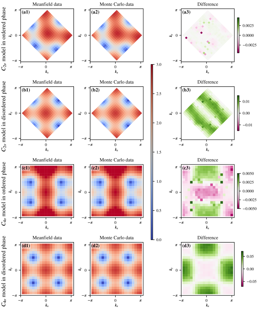
Figure 14: Testing the dispersion of the fermionic single particle gap obtained from Monte Carlo data against mean field results. The first column shows the mean field results according to Eg. (44), while the second column shows numerical results obtained by employing Eq. (72) and the last column shows mean field minus Monte Carlo results. (a) $C_{2v}$ model in ordered phase, at $h=1.0$. The value of the mean field parameter $\phi$ is set to $\langle s^{z}\rangle$ from the Monte Carlo simulation. (b) $C_{2v}$ model in disordered phase, at $h=5.0$. The value of the mean field parameter is set to $\phi=0$. (c) Same as (a), but for the $C_{4v}$ model. (d) Same as (b), but for the $C_{4v}$ model.

VII.2.2 Fermi velocity anisotropy $v_{\perp}/v_{\parallel}$

With $\Delta_{\text{sp}}(\bm{k})$ we can extract the anisotropy at the nodal points $\bm{K}$, via,

$$\frac{v_{\perp}}{v_{\parallel}} =\lim_{\delta\rightarrow 0}\frac{\Delta_{\text{sp}}(\bm{K}+\delta\bm{e}_{\perp})-\Delta_{\text{sp}}(\bm{K})}{\Delta_{\text{sp}}(\bm{K}+\delta\bm{e}_{\parallel})-\Delta_{\text{sp}}(\bm{K})}.$$ (73)

Where $\bm{e}_{\perp}$ and $\bm{e}_{\parallel}$ are unit vectors perpendicular and parallel to the meandering direction of the Dirac cones. We have considered three different strategies for approaching this limit on the finite size lattices, that are all equivalent in the thermodynamic limit:

1. The direct approach:

The most straightforward implementation of Eq. (73) on a finite lattice would be

$$\frac{v_{\perp}}{v_{\parallel}} =\frac{\Delta_{\text{sp}}(\bm{K}+\bm{\delta}_{\perp})-\Delta_{\text{sp}}(\bm{K})}{\Delta_{\text{sp}}(\bm{K}+\bm{\delta}_{\parallel})-\Delta_{\text{sp}}(\bm{K})},$$ (74)

where $\bm{\delta}_{\perp}$, $\bm{\delta}_{\parallel}$ are the shortest distances from the nodal point on the finite-size $\bm{k}$-Lattice.

2. Manually setting the finite size gap $\Delta_{\text{sp}}(\bm{K})=0$:

This approach makes sense, since we know that in the themordynamic limit the gap vanishes. With this strategy, Eq. (73) takes the form

$$\frac{v_{\perp}}{v_{\parallel}} =\frac{\Delta_{\text{sp}}(\bm{K}+\bm{\delta}_{\perp})}{\Delta_{\text{sp}}(\bm{K}+\bm{\delta}_{\parallel})}.$$ (75)

3. Avoid the nodal points:

Another approach for avoiding the finite size gap is to measure one step away from it:

$$\frac{v_{\perp}}{v_{\parallel}} =\frac{\Delta_{\text{sp}}(\bm{K}+2\bm{\delta}_{\perp})-\Delta_{\text{sp}}(\bm{K}+\bm{\delta}_{\perp})}{\Delta_{\text{sp}}(\bm{K}+2\bm{\delta}_{\parallel})-\Delta_{\text{sp}}(\bm{K}+\bm{\delta}_{\parallel})},$$ (76)

The results for these different approaches are shown in Fig. 15. The third strategy results in velocity anisotropies $<1$, while Fig. 2(c) in the main text clearly shows that $v_{\perp}/v_{\parallel}>1$ at the critical point. This implies that the approach strongly underestimates the anisotropy due to the fact that the considered lattices sizes are too small for not measuring directly at the nodal point.

The other two approaches, while not giving quantitatively the same results, are qualitatively equivalent. We have opted to use the second strategy, corresponding to Eq. (75).

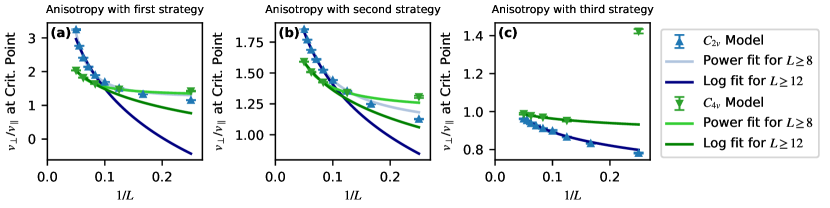
Figure 15: Fermi velocity anisotropy at the critical point as function of $1/L$, determined with (a): Eq. (74), (b): Eq. (75), (c): Eq. (76). Power law and logarithmic fits are shown, except for (c), where only a logarithmic fit is performed.

VIII Critical exponents

VIII.1 Correlation length exponent $\nu$ from RG invariant quantities.

A renormalization group quantity, $R$, has by definition a vanishing scaling dimension. Consider a system at temperature $\beta$, of size $L_{+}\times L_{-}$ with a single relevant coupling $h$. Under a renormalization group transformation that rescales $L_{+}\rightarrow L_{+}/b$ with $b>1$, we expect [43]:

$$R((h-h_{c}),\beta,L_{+},L_{-})=R((h-h_{c})^{\prime},\beta/b^{z},L_{+}/b,L_{-}/b^{1+\Delta z}).$$ (77)

In the above $\Delta z\neq 0$ encodes the difference in scaling between the the $L_{+}$ and $L_{-}$ directions. Linearization of the RG transformation, $(h-h_{c})^{\prime}=b^{1/\nu}(h-h_{c})$ and setting the scale $b=L$ as well as $L_{-}=L_{+}=L$, in accordance to our simulations, yields:

$$R\left((h-h_{c}),\beta,L\right)=f\left(L^{1/\nu}(h-h_{c}),L^{z}/\beta,L^{-\Delta z},L^{-\omega}\right).$$ (78)

In the above we have accounted for possible corrections to scaling $L^{-\omega}$. In the presence of a single length scale $\Delta z=0$, such that the generic finite size scaling form is recovered.

Since in our simulations the temperature is representative of the ground state, we can neglect the dependence on $L^{z}/\beta$. Up to corrections to scaling, $\omega$, and the possibility of $\Delta z\neq 0$, which would result in another correction to scaling term, the data for different lattice sizes cross at the critical field $h_{\mathrm{c}}$ and should collapse when plotted as function of $(h-h_{c})L^{1/\nu}$. The results for such data collapses are shown in Tables 1, 2. Furthermore, Fig. 16 shows $1/\nu$ for the $C_{2v}$ and $C_{4v}$ models from pairwise data collapse of RG-invariant quantities, using system sizes $L$ and $L+2$ ($L+4$). Both suggest a relatively well converged result for $L\geq 12$. Although seemingly converged, our system sizes are too small to detect a logarithmic drift in the exponents.

Table 1: Data collapse results for RG-invariant quantities of $C_{2v}$ model.

Observables	Used system sizes	$h_{c}$	$1/\nu$	$\chi^{2}$
$R_{S}$	8, 10, 12, 14, 16, 18, 20	$3.272715\pm 0.000074$	$1.358934\pm 0.001824$	2.4
$R_{S}$	10, 12, 14, 16, 18, 20	$3.272222\pm 0.000065$	$1.373499\pm 0.002887$	1.8
$R_{S}$	12, 14, 16, 18, 20	$3.272304\pm 0.000099$	$1.376110\pm 0.006104$	1.9
$R_{S}$	14, 16, 18, 20	$3.272617\pm 0.000138$	$1.375085\pm 0.007038$	1.8
$R_{S}$	16, 18, 20	$3.272521\pm 0.000274$	$1.368184\pm 0.014756$	1.9
$R_{S}$	18, 20	$3.273322\pm 0.000449$	$1.373454\pm 0.022000$	1.9
$B$	8, 10, 12, 14, 16, 18, 20	$3.270955\pm 0.000089$	$1.317011\pm 0.002273$	13.4
$B$	10, 12, 14, 16, 18, 20	$3.271532\pm 0.000141$	$1.344485\pm 0.004371$	4.6
$B$	12, 14, 16, 18, 20	$3.272535\pm 0.000175$	$1.352409\pm 0.006242$	3.0
$B$	14, 16, 18, 20	$3.273181\pm 0.000152$	$1.361056\pm 0.007298$	2.6
$B$	16, 18, 20	$3.273783\pm 0.000210$	$1.370788\pm 0.013022$	2.2
$B$	18, 20	$3.274325\pm 0.000464$	$1.340845\pm 0.028414$	1.8
$R_{\chi}$	8, 10, 12, 14, 16, 18, 20	$3.281138\pm 0.000030$	$1.421387\pm 0.000002$	22.0
$R_{\chi}$	10, 12, 14, 16, 18, 20	$3.279752\pm 0.000073$	$1.381046\pm 0.000002$	7.3
$R_{\chi}$	12, 14, 16, 18, 20	$3.275155\pm 0.000500$	$1.369774\pm 0.001609$	5.8
$R_{\chi}$	14, 16, 18, 20	$3.277021\pm 0.000233$	$1.338662\pm 0.010808$	2.2
$R_{\chi}$	16, 18, 20	$3.276434\pm 0.000176$	$1.342788\pm 0.004183$	2.2
$R_{\chi}$	18, 20	$3.275856\pm 0.000693$	$1.369095\pm 0.034679$	2.4

Table 2: Data collapse results for RG-invarian quantities of $C_{4v}$ model.

Observables	Used system sizes	$h_{c}$	$1/\nu$	$\chi^{2}$
$R_{S}$	8, 12, 16, 20	$3.64606\pm 0.00007$	$1.328\pm 0.006$	18.7
$R_{S}$	12, 16, 20	$3.64886\pm 0.00011$	$1.381\pm 0.011$	3.2
$R_{S}$	16, 20	$3.65108\pm 0.00022$	$1.402\pm 0.023$	1.7
$B$	8, 12, 16, 20	$3.64108\pm 0.00009$	$1.254\pm 0.007$	73.2
$B$	12, 16, 20	$3.64818\pm 0.00012$	$1.340\pm 0.014$	5.1
$B$	16, 20	$3.65138\pm 0.00025$	$1.362\pm 0.026$	1.8
$R_{\chi}$	8, 12, 16, 20	$3.66319\pm 0.00027$	$1.309\pm 0.018$	16.5
$R_{\chi}$	12, 16, 20	$3.65708\pm 0.00031$	$1.368\pm 0.028$	3.1
$R_{\chi}$	16, 20	$3.65537\pm 0.00070$	$1.428\pm 0.092$	2.4

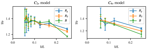
Figure 16: Critical exponent $1/\nu$ of $C_{2v}$ ($C_{4v}$) model from pairwise data collapse of RG-invariant quantities, using linear system sizes $L$ and $L+2$ ($L+4$).

VIII.2 Scaling dimensions and scaling anisotropy

Next, we examine the scaling dimension of the bosonic field from the Ising spin correlations:

$$S(\bm{x})=\Braket{\hat{s}^{z}_{\bf R}(\tau)\hat{s}^{z}_{{\bf 0}}(0)}$$ (79)

where $\bm{x}=(\bm{R},\tau)$ is a space-time coordinate. The models considered in this research are not Lorentz invariant such that the scaling dimension acquires a direction dependence. Following Eq. (78) we expect:

$$S\left(r\hat{\bm{d}}_{*},h\right)\propto\frac{1}{|r\hat{\bm{d}}_{*}|^{2\Delta_{s,*}}}f\left(L^{z}/\beta,(h-h_{c})L^{1/\nu},L^{-\Delta z},L^{-\omega}\right)$$ (80)

where $\hat{\bm{d}}_{*}$ defines the direction.

To determine the scaling dimensions, we consider $S(L\hat{\bm{d}}_{*},h)$, for different system sizes $L$ and use an RG-invariant quantity $R$ to replace in leading order $f(L^{z}/\beta,(h-h_{c})L^{1/\nu},L^{-\Delta z},L^{-\omega})=\tilde{f}(R)$. Using this form, we perform data collapses using system sizes $L$ and $L+2$ ($L$ and $L+4$), where the only free parameter is $\Delta_{s,*}$. The considered directions are defined in Table 3, the $C_{4v}$ symmetry of the second model enforces $\Delta_{s,x}=\Delta_{s,y}$ and $\Delta_{s,+}=\Delta_{s,-}$. As the results in Figs. 17 and 19 show, we cannot resolve a scaling anisotropy between the chosen directions. We conjecture that anisotropies in the exponents will emerge in the infrared limit. Given the very slow flow we believe that our numerical simulations are not in a position to probe these energy scales.

Table 3: Considered directions for the scaling dimension.

$*$	$\hat{\bm{d}}_{*}$
$x$	$(\hat{\bm{e}}_{x},0)$
$y$	$(\hat{\bm{e}}_{y},0)$
$+$	$\frac{1}{2}(\hat{\bm{e}}_{x}+\hat{\bm{e}}_{y},0)$
$-$	$\frac{1}{2}(\hat{\bm{e}}_{x}-\hat{\bm{e}}_{y},0)$
$\tau$	$(\bm{0},0.3)$

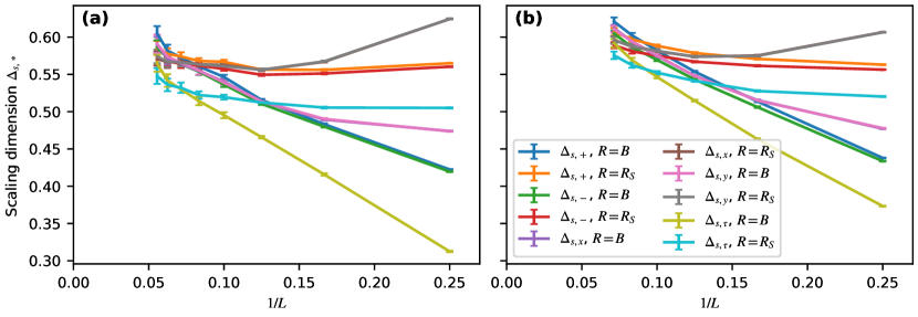
Figure 17: Scaling dimension of Ising field of $C_{2v}$ model. For (a) $\xi=0.25$, (b) $\xi=0.4$. Note: $\Delta_{s,y}$, $R=B$ is indistinguishable from $\Delta_{s,x}$, $R=B$ and $\Delta_{s,y}$, $R=R_{S}$ is identical to $\Delta_{s,x}$, $R=R_{S}$.

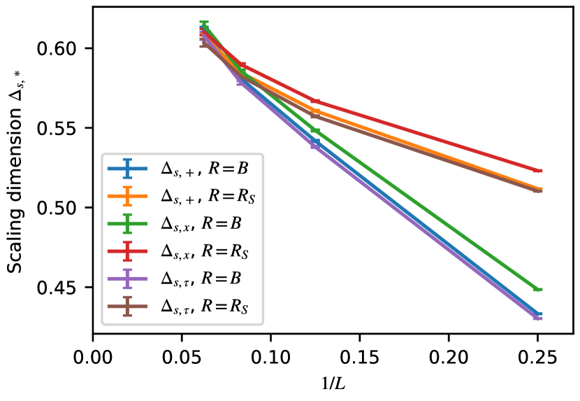
Figure 18: Scaling dimension of Ising field of $C_{4v}$ model.

 

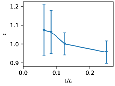
Figure 19: Dynamical exponent $z$ of $C_{4v}$ model.

VIII.3 Dynamical exponent $z$

To determine the dynamical exponent of the $C_{4v}$ model, assume isotropic scaling in space, as suggested by the RG analysis. Then the RG-invariant quantities follow a the critical point the form

$$R=f(L^{z}/\beta,(h-h_{c})L^{1/\nu},L^{-\omega}).$$ (81)

At the crossing points $h_{*}(L)$, with $R(h_{*}(L),L)=R(h_{*}(L),L+\Delta_{L})$ and $\Delta_{L}=4$, we measure $R(\beta)$. Omitting corrections to scaling leads to $R(L,\beta)=f(L^{z}/\beta)$. From this we derive

$$z=\frac{\log\left(\frac{\partial_{\beta}R(L)}{\partial_{\beta}R(L+\Delta_{L})}\right)}{\log\left(\frac{L+\Delta_{L}}{L}\right))}.$$ (82)

The results are shown in Fig. 19, and are consistent with $z=1$ as suggested in the RG analysis.

IX Odd-even effects

The $C_{4v}$ model, has strong odd-even effects. For linear system sizes $L\in 4\mathbb{N}$ ($\equiv$even) and periodic boundary conditions, the Dirac points are included in the discrete set of $\bm{k}$ vectors. This is not the case for odd lattices, $L\in 4\mathbb{N}+2$. Interestingly, the value of the Binder and correlation ratios depend on this choice of the boundary, see Fig. 20(b),(c),(d)). We believe that this stems form the fact that both quantities do not have a well defined thermodynamic limit at $h=h_{c}$. i.e. $\lim_{L\rightarrow\infty}R_{O}(h=h_{c})$ is mathematically not defined. However, the free energy, see Fig. 20(a), the critical field, see Fig. 21(a) the exponents, see Figs. 21(b-d), should ultimately converge to the same value. For odd lattices corrections to scaling are larger.

The critical exponents $2\beta/\nu$ and $\eta$ in Figs. 21(c,d), stem from the scaling assumptions

$$S(\bm{k}=0,h=h_{c},L) \propto L^{2\beta/\nu}, \chi(\bm{k}=0,h=h_{c},L) \propto L^{2-\eta_{\phi}}$$ (83)

where we omitted, as before, the dependence on the inverse temperature $\beta$ and on corrections to scaling. Replacing $h_{c}$ by the crossing point $h_{*}(L)$ of an RG-invariant quantity $R$, meaning $R(h_{*}(L),L)=R(h_{*}(L),L+4)$ with $R\in\{R_{S},R_{\chi},B\}$, we obtain:

$$2\beta/\nu =\log\left(\frac{S(\bm{k}=0,L+4,h=h_{*}(L)}{S(\bm{k}=0,L,h=h_{*}(L)}\right)/\log\left(\frac{L+4}{L}\right),$$ (84)

$$\eta_{\phi} =2-\log\left(\frac{\chi(\bm{k}=0,L+4,h=h_{*}(L)}{\chi(\bm{k}=0,L,h=h_{*}(L)}\right)/\log\left(\frac{L+4}{L}\right).$$ (85)

As apparent in Fig. 21, $h_{c}$ has the smallest corrections to scaling when determined from $R_{S}$. However the smallest corrections to scaling are when determining the critical exponents $2\beta/\nu$, $\eta_{\phi}$ and $z$, are obtained by using $h_{c}$ as determined from $R_{\chi}$. Finally, the velocity anisotropy at the critical point grows in both cases, but is much smaller for odd system sizes, Fig. 22.

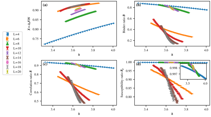
Figure 20: Derivative of free energy and three RG-invariant quantities, showing a continuous transition around $h\approx 3.65$. Notable is an odd-even effect between linear system sizes $L\in 4\mathbb{N}$ (=even) and $L\in 4\mathbb{N}+2$ (=odd).

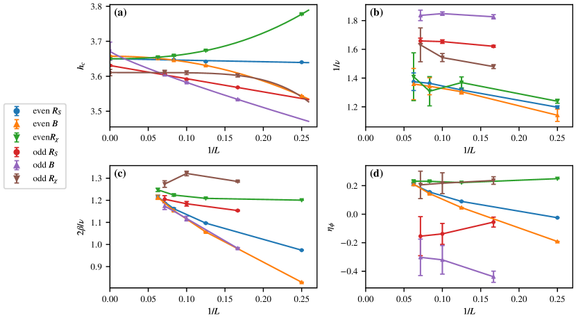
Figure 21: Demonstration of odd-even effects for the $C_{4v}$ model. a: Critical field $h_{c}$, extracted from the three RG-invariant quantities as determined by the crossing points between linear system sizes $L$ and $L+4$. Odd and even system sizes show different behavior. Even system size shows better convergence. b: Critical exponent $1/\nu$ as determined by data collapse of the three RG-invariant quantities, correlation ratio $R$, Binder ratio $B$ and susceptibility ratio $R_{\chi}$, for linear system sizes $L$ and $L+4$. Odd and even system sizes show different behavior. Even system size shows better convergence. c: Critical exponent $2\beta/\nu$ as determined with Eq. 84. d: Critical exponent $\eta_{\phi}$ as determined with Eq. 85.

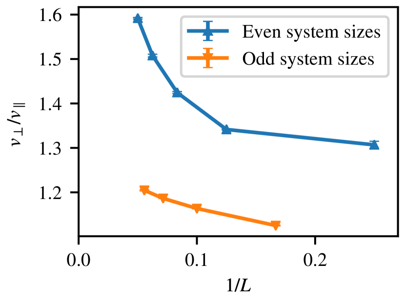
Figure 22: Odd-even effects for the $C_{4v}$ model on the anisotropy velocity of Dirac cones at the critical point.

X Other values for $N_{\sigma}$ and $\xi$

In this section, we report the result of additional simulations for different values of $N_{\sigma}$ and $\xi$. For the $C_{2v}$ model, we show how at higher couplings, $\xi$, discontinuities occur due to level crossings, as already described in Sec. IV. For the $C_{4v}$ model, we show that the transition stays continuous for all considered parameters.

X.1 The $C_{2v}$ model

Fig. 23 shows the structure factor correlation ratio and derivative of free energy for the $C_{2v}$ model at $N_{\sigma}=4$ and $\xi\in\{0.25,0.4,0.5\}$. For these parameters we observe a continuous phase transition. Fig. 24 plots the same observables for $N_{\sigma}=2$. For lower values of the coupling $\xi$ the curves are also smooth, but at $\xi=0.5$ discontinuities appear, which get more pronounced at $\xi=0.75$. At $\xi=0.75$, one can observe multiple discontinuities for a single system size, e.g. at $h\approx 4.2$ and $h\approx 4.4$ for $L=20$. These discontinuities occur due to level crossings, as already described in the mean field part in Sec. IV. As shown in Fig. 24(d,f) and elaborated in the mean field section, they can be avoided by twisting the boundary conditions of the fermionic degrees of freedom.

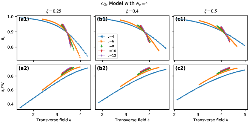
Figure 23: Structure factor correlation ratio and derivative of free energy for the $C_{2v}$ model at $N_{\sigma}=4$ and $\xi\in\{0.25,0.4,0.5\}$. The data is consistent with continuous transitions.

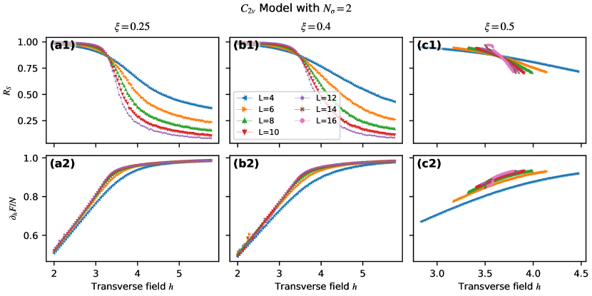
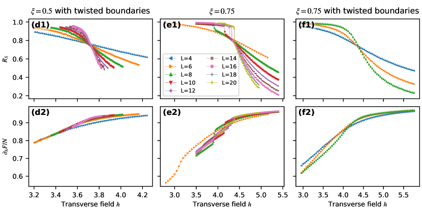
Figure 24: Structure factor correlation ratio and derivative of free energy for the $C_{2v}$ model at $N_{\sigma}=2$ and $\xi\in\{0.25,0.4,0.5,0.75\}$. At $\xi=0.5$ and $\xi=0.75$ discontinuities due to level crossing emerge. They can be avoided by twisting the boundary conditions of the fermionic degrees of freedom.

X.2 The $C_{4v}$ model

Figs. 25,26 have the same layout as the previous figures and show only continuous transitions for various combinations of $N_{\sigma}\in\{1,2\}$, $\xi\in\{0.5,0.75,1,2\}$. We also show data at $\xi=0$, which corresponds to the transverse-field Ising model.

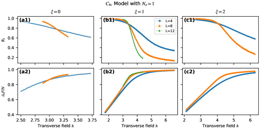
Figure 25: Structure factor correlation ratio and derivative of free energy for the $C_{4v}$ model at $N_{\sigma}=1$ and $\xi\in\{0,1,2\}$. The data shows continuous transitions.

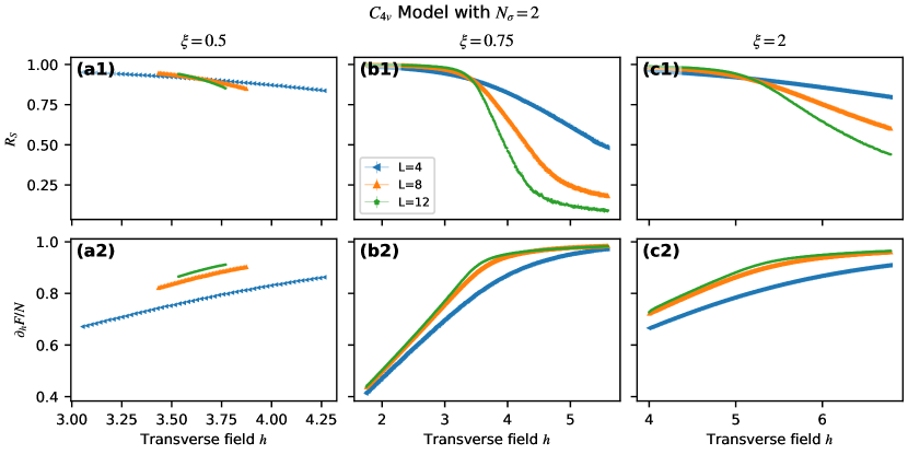
Figure 26: Structure factor correlation ratio and derivative of free energy of the $C_{4v}$ model at $N_{\sigma}=2$ and $\xi\in\{0.5,0.75,2\}$. The data shows continuous transitions.

References

- Sachdev [2011] S. Sachdev, Quantum Phase Transitions, 2nd ed. (Cambridge University Press, Cambridge, 2011).
- Sachdev [2003] S. Sachdev, Colloquium: Order and quantum phase transitions in the cuprate superconductors, Rev. Mod. Phys. 75, 913 (2003).
- v. Löhneysen et al. [2007] H. v. Löhneysen, A. Rosch, M. Vojta, and P. Wölfle, Fermi-liquid instabilities at magnetic quantum phase transitions, Rev. Mod. Phys. 79, 1015 (2007).
- Ryu et al. [2009] S. Ryu, C. Mudry, C.-Y. Hou, and C. Chamon, Masses in graphenelike two-dimensional electronic systems: Topological defects in order parameters and their fractional exchange statistics, Phys. Rev. B 80, 205319 (2009).
- Gross and Neveu [1974] D. J. Gross and A. Neveu, Dynamical symmetry breaking in asymptotically free field theories, Phys. Rev. D 10, 3235 (1974).
- Herbut [2006] I. F. Herbut, Interactions and Phase Transitions on Graphene’s Honeycomb Lattice, Phys. Rev. Lett. 97, 146401 (2006).
- Herbut et al. [2009] I. F. Herbut, V. Juričić, and O. Vafek, Relativistic Mott criticality in graphene, Phys. Rev. B 80, 075432 (2009).
- Janssen and Herbut [2014] L. Janssen and I. F. Herbut, Antiferromagnetic critical point on graphene’s honeycomb lattice: A functional renormalization group approach, Phys. Rev. B 89, 205403 (2014).
- Zerf et al. [2017] N. Zerf, L. N. Mihaila, P. Marquard, I. F. Herbut, and M. M. Scherer, Four-loop critical exponents for the Gross-Neveu-Yukawa models, Phys. Rev. D 96, 096010 (2017).
- Janssen et al. [2018] L. Janssen, I. F. Herbut, and M. M. Scherer, Compatible orders and fermion-induced emergent symmetry in Dirac systems, Phys. Rev. B 97, 041117 (2018).
- Ray et al. [2021] S. Ray, B. Ihrig, D. Kruti, J. A. Gracey, M. M. Scherer, and L. Janssen, Fractionalized quantum criticality in spin-orbital liquids from field theory beyond the leading order, Phys. Rev. B 103, 155160 (2021).
- Oganesyan et al. [2001] V. Oganesyan, S. A. Kivelson, and E. Fradkin, Quantum theory of a nematic Fermi fluid, Phys. Rev. B 64, 195109 (2001).
- Schattner et al. [2016] Y. Schattner, S. Lederer, S. A. Kivelson, and E. Berg, Ising Nematic Quantum Critical Point in a Metal: A Monte Carlo Study, Phys. Rev. X 6, 031028 (2016).
- Vojta et al. [2000a] M. Vojta, Y. Zhang, and S. Sachdev, Quantum Phase Transitions in -Wave Superconductors, Phys. Rev. Lett. 85, 4940 (2000a).
- Vojta et al. [2000b] M. Vojta, Y. Zhang, and S. Sachdev, Renormalization group analysis of quantum critical points in -wave superconductors, Int. J. Mod. Phys. B 14, 3719 (2000b).
- Huh and Sachdev [2008] Y. Huh and S. Sachdev, Renormalization group theory of nematic ordering in -wave superconductors, Phys. Rev. B 78, 064512 (2008).
- Kim et al. [2008] E.-A. Kim, M. J. Lawler, P. Oreto, S. Sachdev, E. Fradkin, and S. A. Kivelson, Theory of the nodal nematic quantum phase transition in superconductors, Phys. Rev. B 77, 184514 (2008).
- Wang [2013] J. Wang, Velocity renormalization of nodal quasiparticles in -wave superconductors, Phys. Rev. B 87, 054511 (2013).
- Ray and Janssen [2021] S. Ray and L. Janssen, Gross-Neveu-Heisenberg criticality from competing nematic and antiferromagnetic orders in bilayer graphene, Phys. Rev. B 104, 045101 (2021).
- Xu et al. [2017] X. Y. Xu, K. Sun, Y. Schattner, E. Berg, and Z. Y. Meng, Non-Fermi Liquid at () Ferromagnetic Quantum Critical Point, Phys. Rev. X 7, 031058 (2017).
- He et al. [2018] Y.-Y. He, X. Y. Xu, K. Sun, F. F. Assaad, Z. Y. Meng, and Z.-Y. Lu, Dynamical generation of topological masses in Dirac fermions, Phys. Rev. B 97, 081110(R) (2018).
- [22] See Supplemental Material, which includes [37, 38, 39, 40, 41, 42, 43].
- Meng et al. [2012] T. Meng, A. Rosch, and M. Garst, Quantum criticality with multiple dynamics, Phys. Rev. B 86, 125107 (2012).
- Janssen and Herbut [2015] L. Janssen and I. F. Herbut, Nematic quantum criticality in three-dimensional Fermi system with quadratic band touching, Phys. Rev. B 92, 045117 (2015).
- Herbut [2007] I. Herbut, A Modern Approach to Critical Phenomena (Cambridge University Press, Cambridge, 2007).
- Liu et al. [2020] Y. Liu, W. Wang, K. Sun, and Z. Y. Meng, Designer Monte Carlo simulation for the Gross-Neveu-Yukawa transition, Phys. Rev. B 101, 064308 (2020).
- Roy et al. [2016] B. Roy, V. Juričić, and I. F. Herbut, Emergent Lorentz symmetry near fermionic quantum critical points in two and three dimensions, J. High Energ. Phys. 04 (2016) 18.
- Nahum et al. [2015] A. Nahum, J. T. Chalker, P. Serna, M. Ortuño, and A. M. Somoza, Deconfined Quantum Criticality, Scaling Violations, and Classical Loop Models, Phys. Rev. X 5, 041048 (2015).
- Nahum [2020] A. Nahum, Note on Wess-Zumino-Witten models and quasiuniversality in dimensions, Phys. Rev. B 102, 201116 (2020).
- ALF Collaboration et al. [2020] ALF Collaboration, F. F. Assaad, M. Bercx, F. Goth, A. Götz, J. S. Hofmann, E. Huffman, Z. Liu, F. Parisen Toldin, J. S. E. Portela, and J. Schwab, The ALF (Algorithms for Lattice Fermions) project release 2.0. Documentation for the auxiliary-field quantum Monte Carlo code, arXiv:2012.11914 (2020).
- Blankenbecler et al. [1981] R. Blankenbecler, D. J. Scalapino, and R. L. Sugar, Monte Carlo calculations of coupled boson-fermion systems., Phys. Rev. D 24, 2278 (1981).
- White et al. [1989] S. R. White, D. J. Scalapino, R. L. Sugar, E. Y. Loh, J. E. Gubernatis, and R. T. Scalettar, Numerical study of the two-dimensional Hubbard model, Phys. Rev. B 40, 506 (1989).
- Assaad and Evertz [2008] F. Assaad and H. Evertz, in Computational Many-Particle Physics, Lect. Notes Phys., Vol. 739, edited by H. Fehske, R. Schneider, and A. Weiße (Springer, Berlin Heidelberg, 2008) pp. 277–356.
- Li et al. [2016] Z.-X. Li, Y.-F. Jiang, and H. Yao, Majorana-Time-Reversal Symmetries: A Fundamental Principle for Sign-Problem-Free Quantum Monte Carlo Simulations, Phys. Rev. Lett. 117, 267002 (2016).
- Kaul [2015] R. K. Kaul, Spin Nematics, Valence-Bond Solids, and Spin Liquids in Quantum Spin Models on the Triangular Lattice, Phys. Rev. Lett. 115, 157202 (2015).
- Liu et al. [2019] Z. H. Liu, X. Y. Xu, Y. Qi, K. Sun, and Z. Y. Meng, Elective-momentum ultrasize quantum Monte Carlo method, Phys. Rev. B 99, 085114 (2019).
- Li et al. [2015] Z.-X. Li, Y.-F. Jiang, and H. Yao, Fermion-sign-free Majarana-quantum-Monte-Carlo studies of quantum critical phenomena of Dirac fermions in two dimensions, New Journal of Physics 17, 085003 (2015).
- Huffman and Chandrasekharan [2014] E. F. Huffman and S. Chandrasekharan, Solution to sign problems in half-filled spin-polarized electronic systems, Phys. Rev. B 89, 111101(R) (2014).
- Wu and Zhang [2005] C. Wu and S.-C. Zhang, Sufficient condition for absence of the sign problem in the fermionic quantum Monte Carlo algorithm, Phys. Rev. B 71, 155115 (2005).
- Scalapino et al. [1993] D. J. Scalapino, S. R. White, and S. Zhang, Insulator, metal, or superconductor: The criteria, Phys. Rev. B 47, 7995 (1993).
- Assaad et al. [1994] F. F. Assaad, W. Hanke, and D. J. Scalapino, Temperature derivative of the superfluid density and flux quantization as criteria for superconductivity in two-dimensional Hubbard models, Phys. Rev. B 50, 12835 (1994).
- Herbut and Janssen [2014] I. F. Herbut and L. Janssen, Topological Mott Insulator in Three-Dimensional Systems with Quadratic Band Touching, Phys. Rev. Lett. 113, 106401 (2014).
- Goldenfeld [1992] N. Goldenfeld, Lectures on Phase Transitions and the Renormalization Group (1st ed.) (CRC Press, Boca Raton, Florida, (1992)).