A Bayesian accelerated failure time model for interval censored three-state screening outcomes

Abstract

Women infected by the Human papilloma virus are at an increased risk to develop cervical intraepithelial neoplasia lesions (CIN). CIN are classified into three grades of increasing severity (CIN-1, CIN-2, and CIN-3) and can eventually develop into cervical cancer. The main purpose of screening is detecting CIN-2 and CIN-3 cases which are usually removed surgically. Screening data from the POBASCAM trial involving 1,454 HPV-positive women are analyzed with two objectives: estimate (a) the transition time from HPV diagnosis to CIN-3; and (b) the transition time from CIN-2 to CIN-3. The screening data have two key characteristics. First, the CIN state is monitored in an interval censored sequence of screening times. Second, a woman’s progression to CIN-3 is only observed if the woman progresses to, both, CIN-2 and from CIN-2 to CIN-3 in the same screening interval. We propose a Bayesian accelerated failure time model for the two transition times in this three-state model. To deal with the unusual censoring structure of the screening data, we develop a Metropolis-within-Gibbs algorithm with data augmentation from the truncated transition time distributions.

1 Introduction

Human papilloma virus (HPV) infections are considered the prime cause of cervical cancer, one of the most common cancers in young women world-wide. After the infection has been acquired through sexual contact, a woman is at risk to develop cervical intraepithelial neoplasia (CIN) lesions in the subsequent years, which can eventually develop into cervical cancer. CIN are classified into three grades of increasing severity: CIN-1, CIN-2, and CIN-3. Treatment is recommended for CIN-2 and CIN-3, but CIN-2 is considered an ambiguous diagnosis and many CIN-2 cases are thought to cure spontaneously without treatment. Hence, CIN-3 is the primary target for detection and treatment in cervical cancer screening programs. For designing screening programs it is essential to have information on two time distributions: (a) the total transition time from HPV diagnosis (state 1) to CIN-3 (state 3) which can be used to optimize screening schedules at the time of expected transition; and (b) the transition time from CIN-2 (state 2) to CIN-3 (state 3) which can be used to judge the speed of transition to CIN-3.

To estimate these transition times, we re-analyze 1,454 HPV-positive women, recruited between 1999 and 2002 in the Population Based Screening Study Amsterdam (POBASCAM; Rijkaart et al., 2012; Dijkstra et al., 2016). Participants were screened for CIN progression at multiple occasions yielding a series of interval censored observations of the disease status. The key characteristic of screening data, like POBASCAM, is their censoring structure: after a woman is diagnosed with CIN-2, the lesion is radically removed and the screening series is censored, since the patient’s progression from CIN-2 to CIN-3 cannot be observed anymore. As a consequence, CIN-3 is found only in those women who progress to, both, CIN-2 and from CIN-2 to CIN-3 in the same time interval.

Figure 1: Censoring structure in the present study. The arrows represent three timelines for a person $i$ with transition times $y_{i}=x_{i}+t_{i}$. Superimposed are three hypothetical screening sequences with screening times $(v_{i,1},v_{i,2},v_{i,3})$ leading to the censoring states $\delta_{i}\in\{1,2,3\}$, corresponding to HPV+, CIN-2, and CIN-3. The coding of the censoring interval $\phi_{i}=(l_{i},r_{i}]$ is shown on the right.

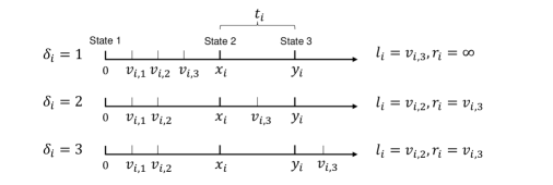
The type of screening data considered in the present study follow a progressive three-state model, where state 2 (CIN-2) follows state 1 (HPV infection), and state 3 (CIN-3) follows state 2 (CIN-2). In a sample of individuals, $i=1,...,n$, the latent onset transition time from state 1 to 2 is $x_{i}$ and the progression transition time from state 2 to state 3 is $t_{i}$, where the total transition time is $y_{i}=x_{i}+t_{i}$. In Figure 1, we superimpose three hypothetical sequences of screening times $(v_{i,1},v_{i,2},v_{i,3})$ on this natural disease process yielding the censoring states $\delta_{i}\in\{1,2,3\}$. The screening times may be regular (e.g., planned) or irregular, as shown in Figure 1. For $\delta_{i}=1$, the individual does not progress to state 2 before the last screening moment ($v_{i,3}$), so that the individual is in state 1 at the end of follow-up. We use $\phi_{i}=(l_{i},r_{i}]$ to denote the most recent screening interval and its coding is shown on the right hand of Figure 1. We adopt the convention that if $\delta_{i}=1$, $l_{i}$ is equal to the last screening time ($v_{i,3}$) and $r_{i}=\infty$. For $\delta_{i}=2$, a state 2 event is detected at the last screening time before the individual progresses to state 3 ($v_{i,2}<x_{i}\leq v_{i,3}<y_{i}$). After its detection, CIN-2 is removed and, therefore, we do not observe anymore when the individual would have progressed to CIN-3. For $\delta_{i}=3$, a state 3 event is observed. This implies that the individual has progressed from state 1 to 2 and the individual has continued progression from state 2 to the detected state 3 ($v_{i,2}<x_{i}<y_{i}\leq v_{i,3}$).

In this paper, we develop a Bayesian parametric simultaneous accelerated failure time (AFT) model for the two transition times $x_{i}$ and $t_{i}$. Related methodology is reviewed in Section 2. Our method is novel in that it allows choosing any type of parametric distribution for the transition times. In particular, our model can handle non-constant and non-proportional hazards on both transitions (e.g., Weibull, loglogistic or lognormal distributions). Furthermore, the method is tailored to our censoring setting which is often encountered in screening data. This setting is challenging, since the transition of a woman to CIN-3 is never observed if a CIN-2 lesion is detected during screening, so that estimating $t_{i}$ is hard.

The Bayesian estimation approach is motivated as follows. First, we develop a Markov Chain Monte Carlo (MCMC) algorithm with a general data augmentation step which can handle any parametric transition time distribution, provided its truncated form exists. Through this, different distributions can be ’plugged in’ to the algorithm and standard Bayesian model selection can readily be applied to select the best distributions for the data. We also derive an alternative maximum likelihood (ML) expectation-maximization (EM) estimator to demonstrate that it needs a dedicated implementation for any choice of transition time distributions, rendering it the less flexible approach. Second, we use weakly informative priors to enhance the robustness of parameter estimation through regularization. It is well-known that priors effectively regularize the likelihood and can improve optimization in ill-posed problems (e.g., flat and multi-modal likelihoods) by putting higher weight on a range of realistic values (e.g., Gelman et al., 2008). The benefit of regularization is usually greatest in sparse data settings, which indeed emerge due to our censoring structure when estimating the parameters of the distribution of $t_{i}$. As we show, these parameters are updated only by information from patients experiencing state 2 and 3 events. This problem is aggravated in screening data, where advanced states usually occur infrequently (19% in POBASCAM). We demonstrate that Bayes can outperform ML-EM in such settings. Third, Gibbs sampling facilitates inference on parameters as well as the cumulative incidence functions (CIFs). In contrast, ML-EM requires re-sampling techniques which can be costly due to numerical integration in the E-step.

In the next section, we review related statistical methodology. Subsequently, Sections 3 and 4 present the model, the Bayesian estimation procedure, and the ML-EM algorithm. The proposed method is evaluated in a simulation study (Section 5) and applied to the data from POBASCAM (Section 6). We discuss the results and the methodology in Section 7.

2 Related statistical methodology

A straightforward modeling approach treats the three-state screening data (Figure 1) as univariate interval censored. This approach estimates the distribution of $y_{i}$ by considering an observation right censored at $l_{i}$ if $\delta_{i}=1$, right censored at $r_{i}$ if $\delta_{i}=2$, and interval censored if $\delta_{i}=3$. Furthermore, to estimate the distribution of $x_{i}$ the approach considers $\delta_{i}=2$ and $3$ as the same event. These data could then readily be analyzed by standard survival methods, such as a parametric interval censored survival regression (Jackson, 2016) or the non-parametric maximum likelihood estimator (NPMLE; Turnbull, 1976). However, unfortunately, this approach cannot estimate $t_{i}$ and, in general, fails for $y_{i}$, as it introduces informative interval censoring. This problem emerges, because the re-coding scheme introduces a dependence of the censoring times and $y_{i}$; see proof in the Supplemental Material, Section A.

More tailored methods for modeling screening data are available, in particular multi-state Markov and semi-Markov models (for reviews see, e.g., Mandel, 2010; Asanjarani et al., 2021). Multi-state models differ, broadly, concerning their assumptions on (a) the observation process (i.e., the censoring mechanism) and (b) the transition time distributions. These aspects are interlinked. First, if transitions are discretely observed, as in the present study (i.e., interval censoring, also called panel data), information on the time of transition is limited which may necessitate stronger constraints on the transition time distributions for tractable estimation. In Markov models, exponential distributions have been applied which implies that hazards are constrained to be constant. Consequently, estimation of models with arbitrary transitions and censoring structures is tractable (e.g., Jackson, 2011). However, we find the constant hazard constraint unrealistic, for instance because HPV infections can clear over time.

Second, if the transition times are exactly observed (possibly right or left censored), which they are not in our study, more information is available for modeling distributions with non-constant hazards (semi-Markov models). The R package flexsurv (Jackson, 2016), for example, then allows fitting multi-state models with various parametric survival distributions, while the package mstate (de Wreede et al., 2011) estimates semi-parametric proportional hazards.

Third, the problem of estimating semi-Markov multi-state models with interval censored transitions, addressed in the present study, is challenging, because the involved likelihoods can become intractable (Lange and Minin, 2013). Our Bayesian three-state model can be viewed as a semi-Markov model applying to a specific interval censored observation process (Figure 1) and allowing arbitrary parametric transition time distributions with potentially non-constant and non-proportional hazards by an AFT specification. To the contrary, previous studies have offered tailored solutions for other censoring structures, admissible transitions, or transition time distributions. Progressive three-state models for ’doubly-interval censored’ data, for example, differ from our setting in that each individual has two paired intervals in which $x_{i}$ and $y_{i}$ occur, respectively (De Gruttola and Lagakos, 1989). Komárek and Lesaffre (2008) proposed a Bayesian AFT model for doubly-interval censored three-state models which allows approximation of the transition time distributions by a Gaussian mixture. Similarly, Boruvka and Cook (2016) addressed doubly-interval censoring in an illness-death model by a sieve estimator. Furthermore, several multi-state semi-Markov models have been developed for Weibull transitions (Foucher et al., 2007, 2010; Kang and Lagakos, 2007; Wei and Kryscio, 2016). These models either assumed interval censoring of all events, exactly observed absorbing event times (e.g., death), or they required one transition to be exponentially distributed. While the first two requirements are not met by the three-state screening data in our study, we find the Markov assumption too restrictive.

Finally, an approach suggested by Titman and Sharples (2010) and Lange and Minin (2013) can be applied to approximate semi-Markov transitions in multi-state models by specifying multiple latent Continuous Time Markov Chains (see also Lange et al., 2018). Another approximate method, suggested by Jackson (2011) for the R package msm, allows hazards to change at pre-specified time points (knots), so called piece-wise constant hazards. This approach models time inhomogeneous transitions, but cannot, in general, be used to approximate semi-Markov transitions. The two approximate methods require a priori choices on the type of latent transition structures or the number of knots that should be tried during model fitting. In contrast, the proposed Bayesian approach provides inference for semi-Markov transitions with arbitrary parametric time distributions.

3 Three-state AFT model for screening data

We assume that the random variables $x_{i}$ and $t_{i}$ follow two AFT models

$$\log x_{i}=\operatorname{\mathbf{z}}_{x,i}^{\prime}\operatorname{\bm{\beta}}_{x}+\sigma_{x}\epsilon_{i}$$ (1)

$$\log t_{i}=\operatorname{\mathbf{z}}_{t,i}^{\prime}\operatorname{\bm{\beta}}_{t}+\sigma_{t}\xi_{i}\quad\quad\quad\text{for}\ i=1,...,n,$$ (2)

where $n$ denotes the sample size and $\operatorname{\mathbf{z}}_{i}=\operatorname{\mathbf{z}}_{x,i}\cup\operatorname{\mathbf{z}}_{t,i}$ denotes vectors of covariates of dimensions $(p\times 1)$, $(p_{x}\times 1)$, and $(p_{t}\times 1)$. The unknown regression parameters are $\operatorname{\bm{\beta}}=(\operatorname{\bm{\beta}}_{x}^{\prime},\operatorname{\bm{\beta}}_{t}^{\prime})^{\prime}$ and the unknown scale parameters are $\operatorname{\bm{\sigma}}=(\sigma_{x},\sigma_{t})$. The covariate vectors are understood to include an intercept on the first entry, respectively. We assume the joint density of the random error terms factors $f_{\epsilon,\xi}(\epsilon,\xi)=f_{\epsilon}(\epsilon)f_{\xi}(\xi)$, so that $x_{i}$ and $t_{i}$ are conditionally independent given the covariates $\operatorname{\mathbf{z}}_{i}$, but marginally dependent. The pair $(x_{i},t_{i})$ is never observed so that estimating their association is hard. In the POBASCAM application, we include HPV-sub-types as known important common causes of faster transition in both model equations. In addition, we suggest a sensitivity analysis that relaxes conditional independence; see Section 4.5.

The specific choice of $f_{\epsilon}$ and $f_{\xi}$ determines the distributions of $x_{i}$ and $t_{i}$, obtained by a change of variables

$$f_{x}(x_{i}|\operatorname{\mathbf{z}}_{x,i},\operatorname{\bm{\beta}}_{x},\sigma_{x})=f_{\epsilon}[(\log x_{i}-\operatorname{\mathbf{z}}_{x,i}^{\prime}\operatorname{\bm{\beta}}_{x})\sigma_{x}^{-1}](\sigma_{x}x_{i})^{-1}\quad;x>0$$ (3)

and the density $f_{t}$ follows similarly. Common choices for $f_{\epsilon}$ and $f_{\xi}$ include the extreme value, logistic, and normal distributions, for which $x_{i}$ and $t_{i}$ are distributed Weibull, loglogistic, and lognormal, respectively (Table 1).

Table 1: Error distributions and change of variable in AFT models

Error dist.	$f_{\epsilon}(\epsilon_{i})$	Dist. $x_{i}$	$f_{x}(x_{i})$	Re-parameterization
Extreme value	$\exp(\epsilon_{i}-e^{\epsilon_{i}})$	Weibull	$\frac{\eta}{\gamma}(\frac{x_{i}}{\gamma})^{\eta-1}\exp[-(\frac{x_{i}}{\gamma})^{\eta}]$	$\eta:=\sigma_{x}^{-1}$ ; $\gamma:=\exp(\operatorname{\mathbf{z}}_{x,i}^{\prime}\operatorname{\bm{\beta}}_{x})$
Logistic	$e^{\epsilon_{i}}(1+e^{\epsilon_{i}})^{-2}$	Log-logistic	$\frac{\eta}{\gamma}[\frac{x_{i}}{\gamma}]^{\eta-1}[1+(\frac{x_{i}}{\gamma})^{\eta}]^{-2}$	$\eta:=\sigma_{x}^{-1}$ ; $\gamma:=\exp(\operatorname{\mathbf{z}}_{x,i}^{\prime}\operatorname{\bm{\beta}}_{x})$
Normal	$[\sqrt{2\pi}]^{-1}\exp[-\frac{1}{2}\epsilon_{i}^{2}]$	Log-normal	$[\sigma_{x}x_{i}\sqrt{2\pi}]^{-1}\exp[-(\frac{\log x_{i}-\mu}{\sqrt{2}\sigma_{x}})^{2}]$	$\mu:=\operatorname{\mathbf{z}}_{x,i}^{\prime}\operatorname{\bm{\beta}}_{x}$

3.1 Censoring mechanism

A fixed or random screening process yields a vector of subsequent potential screening times $\operatorname{\mathbf{v}}_{i}=(0,v_{i,1},...,v_{i,m_{i}},\infty)$ with first and last entries set to zero and infinity, respectively, and $m_{i}$ random. We assume non-informative censoring in the sense that $x_{i}$ and $t_{i}$ are independent of $\operatorname{\mathbf{v}}_{i}$, unconditionally or conditionally on the covariates $\operatorname{\mathbf{z}}_{i}$. Then the censoring interval $\phi_{i}=(l_{i},r_{i}]$ is defined such that

$$\Pr(l_{i}=v_{i,j},r_{i}=v_{i,j+1}|x_{i},\operatorname{\mathbf{v}}_{i})=\mathds{1}_{\{v_{i,j}<x_{i}\leq v_{i,j+1}\}}$$ (4)

for $j=1,...,m_{i}$, where $\mathds{1}$ denotes the indicator function; see Komárek and Lesaffre (2008) for a similar definition of interval censoring. The corresponding censoring event is then

$$\delta_{i}=\begin{cases}1\ &\text{if}\ \ l_{i}<x_{i}<r_{i}=\infty\\ 2\ &\text{if}\ \ l_{i}<x_{i}\leq r_{i}<x_{i}+t_{i}\\ 3\ &\text{if}\ \ l_{i}<x_{i}<x_{i}+t_{i}\leq r_{i}<\infty.\end{cases}$$ (5)

Indicator $\delta_{i}$ relates to states 1 (HPV-positive), 2 (CIN-2), and 3 (CIN-3), respectively. The condition $l_{i}<x_{i}$ appears in each level of $\delta_{i}$ and may also be omitted. Observe that indicator $\delta_{i}$ is marginally random, but, conditionally on $x_{i},t_{i}$, and $\phi_{i}$, it is deterministic; for example, $\Pr(\delta_{i}=3|x_{i},t_{i},\phi_{i})=\mathds{1}_{\{x_{i}+t_{i}\leq r_{i}<\infty\}}$.

3.2 Data and prior assumptions

The data observed for individual $i$ are $\mathcal{D}_{i}=\{\operatorname{\mathbf{z}}^{\prime}_{i},\delta_{i},l_{i},r_{i}\}$ and we write $\bm{\mathcal{D}}$ for the stacked $[n\times(p+3)]$ matrix of $i=1,...,n$ independent observations. Although the screening process $\operatorname{\mathbf{v}}_{i}$ is sometimes partly observed, i.e., the screening history $v_{i,1}...v_{i,j-1}$ is known, $\phi_{i}$ is sufficient to identify the posterior distribution, as discussed below.

The model parameters $\operatorname{\bm{\beta}}$ and $\operatorname{\bm{\sigma}}$ are random variables with independent priors

$$\pi(\operatorname{\bm{\beta}},\operatorname{\bm{\sigma}}|\operatorname{\bm{\tau}},\operatorname{\bm{\lambda}})=\pi(\sigma_{x}|\lambda_{x})\pi(\sigma_{t}|\lambda_{t})\bigg{[}\prod_{j=1}^{p_{x}}\pi(\beta_{x,j}|\tau_{x})\bigg{]}\bigg{[}\prod_{k=1}^{p_{t}}\pi(\beta_{t,k}|\tau_{t})\bigg{]},$$ (6)

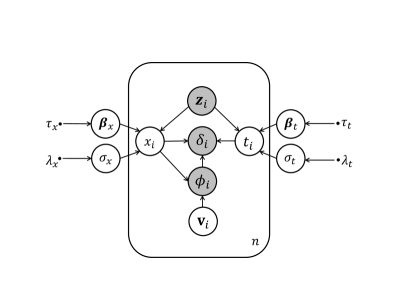
where $\operatorname{\bm{\tau}}=(\tau_{x},\tau_{t})$ and $\operatorname{\bm{\lambda}}=(\lambda_{x},\lambda_{t})$ are the hyperparameters. Figure 2 summarizes the hierarchical structure of the model using plate notation. As argued in Section 1, we use weakly informative priors to regularize parameter estimation. In particular, we set Student’s t-distribution with four degrees of freedom as prior for $\beta_{j}$, i.e., $\pi(\beta_{j}|\tau)=student(\tau=4)$, which encodes the prior expectation that $\beta_{j}$ of a standardized $z_{j}$ lies with 95% probability in (-2.776, 2.776) or $\exp(\beta_{j})$ in $(0.062,16.062)$, approximately, denoting large effects. Still the prior leaves the possibility for very large effects due to its wide tails. Furthermore, we use a half-normal $\pi(\sigma|\lambda)=N^{+}(0,\lambda=\sqrt{10})$ prior (with $\lambda$ the standard deviation) which encodes 95% prior probability in the interval $(0.099,6.198)$. Since the shape of the Weibull and lognormal distributions is governed by $\eta=\sigma^{-1}$ (Table 1), the $\sigma$-prior locates $\eta$ with 95% prior mass in $(0.161,10.091)$. We believe, this prior generally allows very flexible shape of the time distributions. A prior sensitivity analysis is shown in our case study; see Section 6.5.

Figure 2: Graphical illustration of the three-state AFT model using plate notation of directed acyclical graph theory. Circles denote random variables, dots denote fixed variables, and filled circles denote observations. Arrows indicate the direction of causation; for example, $x_{i}$ is generated by $f_{x}(x_{i}|\operatorname{\mathbf{z}}_{i},\operatorname{\bm{\beta}}_{x},\sigma_{x})$.

4 Bayesian estimation

Let $q$ denote a generic density. Let $\operatorname{\mathbf{x}}=(x_{1},...,x_{n})^{\prime},\operatorname{\mathbf{t}}=(t_{1},...,t_{n})^{\prime}$ be $(n\times 1)$ vectors of latent transition times, respectively, and $\operatorname{\{\mathbf{v}\}}=\{\operatorname{\mathbf{v}}_{1},...,\operatorname{\mathbf{v}}_{n}\}$ the set of screening times vectors. Our objective is sampling from the joint posterior distribution

$$q(\operatorname{\bm{\beta}},\operatorname{\bm{\sigma}},\operatorname{\mathbf{x}},\operatorname{\mathbf{t}}|\bm{\mathcal{D}},\operatorname{\{\mathbf{v}\}};\operatorname{\bm{\tau}},\operatorname{\bm{\lambda}})=q(\operatorname{\bm{\beta}},\operatorname{\bm{\sigma}}|\operatorname{\mathbf{x}},\operatorname{\mathbf{t}},\bm{\mathcal{D}},\operatorname{\{\mathbf{v}\}};\operatorname{\bm{\tau}},\operatorname{\bm{\lambda}})q(\operatorname{\mathbf{x}},\operatorname{\mathbf{t}}|\bm{\mathcal{D}},\operatorname{\{\mathbf{v}\}}).$$ (7)

The first factor on the right side of (7) is the complete data posterior which is proportional to the prior, given in (6), times the complete data likelihood, given by

$$L(\operatorname{\bm{\beta}},\operatorname{\bm{\sigma}}|\operatorname{\mathbf{x}},\operatorname{\mathbf{t}},\bm{\mathcal{D}},\operatorname{\{\mathbf{v}\}}) \propto\prod_{i=1}^{n}q(x_{i},t_{i}|\operatorname{\mathbf{z}}_{i},\operatorname{\bm{\beta}},\operatorname{\bm{\sigma}})q(\phi_{i},\delta_{i},\operatorname{\mathbf{v}}_{i}|x_{i},t_{i},\operatorname{\mathbf{z}}_{i},\operatorname{\bm{\beta}},\operatorname{\bm{\sigma}})$$ (8)

$$=\prod_{i=1}^{n}q(x_{i},t_{i}|\operatorname{\mathbf{z}}_{i},\operatorname{\bm{\beta}},\operatorname{\bm{\sigma}})q(\phi_{i},\delta_{i},\operatorname{\mathbf{v}}_{i}|x_{i},t_{i},\operatorname{\mathbf{z}}_{i})$$

$$\propto\prod_{i=1}^{n}f_{x}(x_{i}|\operatorname{\mathbf{z}}_{i},\operatorname{\bm{\beta}}_{x},\sigma_{x})f_{t}(t_{i}|\operatorname{\mathbf{z}}_{i},\operatorname{\bm{\beta}}_{t},\sigma_{t})$$

$$=L(\operatorname{\bm{\beta}}_{x},\sigma_{x}|\operatorname{\mathbf{x}},\operatorname{\mathbf{z}})\times L(\operatorname{\bm{\beta}}_{t},\sigma_{t}|\operatorname{\mathbf{t}},\operatorname{\mathbf{z}}),$$

where $f_{x}$ and $f_{t}$ are defined in (3). We used d-separation based on Figure 2 to establish independence of $\operatorname{\bm{\phi}},\operatorname{\bm{\delta}}$ of the parameters conditional on $\operatorname{\mathbf{x}},\operatorname{\mathbf{t}}$ in the second equation. The third equation results from the assumption of conditional independence. We find that the parameters are identified by the vector of latent times, which, however, are unobserved. Furthermore, the second factor on the right side of (7) is the marginal likelihood of the latent times that is hard to sample directly. Therefore, we employ Gibbs sampling to sample from (7), based on the full conditional distributions of the random variables.

4.1 Gibbs sampling from the full conditional distributions

After suitable initialization of $\{\operatorname{\bm{\beta}},\operatorname{\bm{\sigma}},\operatorname{\mathbf{x}},\operatorname{\mathbf{t}}\}$, the Gibbs sampler proceeds by updating parameters by the following blocks

$$\operatorname{\bm{\beta}}^{(k+1)},\operatorname{\bm{\sigma}}^{(k+1)} \sim q(\operatorname{\bm{\beta}},\operatorname{\bm{\sigma}}|\operatorname{\mathbf{x}}^{(k)},\operatorname{\mathbf{t}}^{(k)},\bm{\mathcal{D}},\operatorname{\{\mathbf{v}\}};\operatorname{\bm{\tau}},\operatorname{\bm{\lambda}})$$ (9)

$$x_{i}^{(k+1)} \sim q(x_{i}|\operatorname{\bm{\beta}}^{(k+1)},\operatorname{\bm{\sigma}}^{(k+1)},t_{i}^{(k)},\mathcal{D}_{i},\operatorname{\mathbf{v}}_{i};\operatorname{\bm{\tau}},\operatorname{\bm{\lambda}}) i=1,...,n$$ (10)

$$t_{i}^{(k+1)} \sim q(t_{i}|\operatorname{\bm{\beta}}^{(k+1)},\operatorname{\bm{\sigma}}^{(k+1)},x_{i}^{(k+1)},\mathcal{D}_{i},\operatorname{\mathbf{v}}_{i};\operatorname{\bm{\tau}},\operatorname{\bm{\lambda}}) i=1,...,n.$$ (11)

We derive the full conditional distributions (9-11) in the following. From (8) it directly follows for (9) that

$$q(\operatorname{\bm{\beta}},\operatorname{\bm{\sigma}}|\operatorname{\mathbf{x}},\operatorname{\mathbf{t}},\bm{\mathcal{D}},\operatorname{\{\mathbf{v}\}};\operatorname{\bm{\tau}},\operatorname{\bm{\lambda}})\propto\ q(\operatorname{\bm{\beta}}_{x},\sigma_{x}|\operatorname{\mathbf{x}},\operatorname{\mathbf{z}};\tau_{x},\lambda_{x})q(\operatorname{\bm{\beta}}_{t},\sigma_{t}|\operatorname{\mathbf{t}},\operatorname{\mathbf{z}};\tau_{t},\lambda_{t}).$$

The step in (9) thus constitutes sampling from the complete data posteriors of two conditionally independent AFT models. In general, the weakly informative priors considered are not conjugate to the likelihoods. Therefore, we use a Metropolis step for sampling ($\operatorname{\bm{\beta}},\operatorname{\bm{\sigma}}$) jointly, applying a multivariate normal proposal distribution $\text{N}(\bm{\mu},\Sigma)$ with $\bm{\mu}$ centered at the previous draw $(\operatorname{\bm{\beta}}^{(k)},\operatorname{\bm{\sigma}}^{(k)})$ and a diagonal proposal variance matrix $\Sigma$.

The steps in (10) and (11) constitute data augmentation of the latent transition times (Albert and Chib, 1993). Proofs of the following results (12-15) are given in the Supplemental Material, Section A. For (10), we have

$$q(x_{i}|\operatorname{\bm{\beta}},\operatorname{\bm{\sigma}},t_{i},\mathcal{D}_{i},\operatorname{\mathbf{v}}_{i};\operatorname{\bm{\tau}},\operatorname{\bm{\lambda}})=f_{x}(x_{i}|a(\phi_{i},\delta_{i},t_{i})<x_{i}<b(\phi_{i},\delta_{i},t_{i}),\operatorname{\mathbf{z}}_{i},\operatorname{\bm{\beta}}_{x},\sigma_{x}),$$ (12)

i.e., the full conditional distribution of $x_{i}$ is a truncated distribution with bounds

$$(a(\phi_{i},\delta_{i},t_{i}),b(\phi_{i},\delta_{i},t_{i}))=\begin{cases}(l_{i},\infty)\quad&\text{if}\ \delta_{i}=1\\ (\max(r_{i}-t_{i},l_{i}),r_{i}]\quad&\text{if}\ \delta_{i}=2\\ (l_{i},r_{i}-t_{i}]\quad&\text{if}\ \delta_{i}=3.\\ \end{cases}$$ (13)

Sampling from the truncated distribution is straight forward because the cumulative distribution $F_{x}$ is known; given $u\sim\text{uniform}(0,1)$, we evaluate $F^{-1}_{x}$ at $F_{x}(a)+u(F_{x}(b)-F_{x}(a))$. Similarly, for the full conditional (11) we have

$$q(t_{i}|\operatorname{\bm{\beta}},\operatorname{\bm{\sigma}},x_{i},\mathcal{D}_{i},\operatorname{\mathbf{v}}_{i};\operatorname{\bm{\tau}},\operatorname{\bm{\lambda}}) =f_{t}(t_{i}|c(\phi_{i},\delta_{i},x_{i})<t_{i}<d(\phi_{i},\delta_{i},x_{i}),\operatorname{\mathbf{z}}_{i},\operatorname{\bm{\beta}}_{t},\sigma_{t})$$ (14)

with truncation bounds:

$$(c(\phi_{i},\delta_{i},x_{i}),d(\phi_{i},\delta_{i},x_{i}))=\begin{cases}(0,\infty)\quad&\text{if}\ \delta_{i}=1\\ (r_{i}-x_{i},\infty)\quad&\text{if}\ \delta_{i}=2\\ (0,r_{i}-x_{i}]\quad&\text{if}\ \delta_{i}=3.\\ \end{cases}$$ (15)

Note that these results imply that (9-11) depend on $\operatorname{\mathbf{v}}_{i}$ only through interval $\phi_{i}$. Posterior sampling, therefore, neither requires the full screening history to be part of the data nor the specification of a distribution for the screening process. Furthermore, we observe from (15) that, for $\delta_{i}=1$, $t_{i}$ is not constrained by the data, i.e., $(c,d)=(0,\infty)$; as a result posterior estimation of $(\operatorname{\bm{\beta}}_{t},\sigma_{t})$ crucially depends on the frequency of $\delta_{i}\in\{2,3\}$, i.e., information for updating $t_{i}$. However, in the POBASCAM data, as in other screening data sets likewise, advanced state events occur infrequently. The Bayesian estimation approach then can benefit from including weak prior information, as described in Sections 1 and 3.2.

Gibbs algorithm (9-11) was implemented in the statistical programming language R as package BayesTSM (Bayesian three-state model), available under https://github.com/thomasklausch2/BayesTSM.

4.2 Maximum likelihood EM-algorithm

Bayesian estimation is compared to an EM-algorithm used to maximize the observed data likelihood

$$L(\operatorname{\bm{\beta}},\operatorname{\bm{\sigma}}|\bm{\mathcal{D}})\propto \prod_{i:\delta_{i}=1}\big{[}1-F_{x}(l_{i}|\operatorname{\mathbf{z}}_{i},\operatorname{\bm{\beta}}_{x},\sigma_{x})\big{]}\times$$ (16)

$$\prod_{i:\delta_{i}=2}\big{[}\int_{l_{i}}^{r_{i}}f_{x}(x_{i}|\operatorname{\mathbf{z}}_{i},\operatorname{\bm{\beta}}_{x},\sigma_{x})[1-F_{t}(r_{i}-x_{i}|\operatorname{\mathbf{z}}_{i},\operatorname{\bm{\beta}}_{t},\sigma_{t})]dx_{i}\big{]}\times$$

$$\prod_{i:\delta_{i}=3}\big{[}\int_{l_{i}}^{r_{i}}f_{x}(x_{i}|\operatorname{\mathbf{z}}_{i},\operatorname{\bm{\beta}}_{x},\sigma_{x})F_{t}(r_{i}-x_{i}|\operatorname{\mathbf{z}}_{i},\operatorname{\bm{\beta}}_{t},\sigma_{t})dx_{i}\big{]}.$$

The three product terms in (16) factorize the probabilities of occurrence of $x_{i}$ and $t_{i}$ in the observed interval $\phi_{i}$ given the observed state $\delta_{i}$. EM finds the maximum of (16) by iterating until convergence

$$(\operatorname{\bm{\beta}}^{(k+1)},\operatorname{\bm{\sigma}}^{(k+1)})=\operatorname*{arg\,max}_{\operatorname{\bm{\beta}},\operatorname{\bm{\sigma}}}\ \big{[} \operatorname{\mathbb{E}}_{x_{i}|\mathcal{D}_{i},\operatorname{\bm{\beta}}^{(k)},\operatorname{\bm{\sigma}}^{(k)}}\big{[}\log L(\operatorname{\bm{\beta}}_{x},\sigma_{x}|\operatorname{\mathbf{x}},\operatorname{\mathbf{z}})\big{]}+$$ (17)

$$\operatorname{\mathbb{E}}_{t_{i}|\mathcal{D}_{i},\operatorname{\bm{\beta}}^{(k)},\operatorname{\bm{\sigma}}^{(k)}}\big{[}\log L(\operatorname{\bm{\beta}}_{t},\sigma_{t}|\operatorname{\mathbf{t}},\operatorname{\mathbf{z}})\big{]}\big{]},$$

where $L(\operatorname{\bm{\beta}}_{x},\sigma_{x}|\operatorname{\mathbf{x}},\operatorname{\mathbf{z}})$ and $L(\operatorname{\bm{\beta}}_{t},\sigma_{t}|\operatorname{\mathbf{t}},\operatorname{\mathbf{z}})$ are the complete data likelihoods in (8). The expectations are taken with respect to the predictive densities $q(x_{i}|\mathcal{D}_{i},\operatorname{\bm{\beta}},\operatorname{\bm{\sigma}})$ and $q(t_{i}|\mathcal{D}_{i},\operatorname{\bm{\beta}},\operatorname{\bm{\sigma}})$, which are similar to the full conditional densities in (10-11), but do not condition on $t_{i}$ and $x_{i}$, respectively. In the Supplemental Material, Section A, we prove that

$$q(x_{i}|\mathcal{D}_{i},\operatorname{\bm{\beta}},\operatorname{\bm{\sigma}})\propto g_{x}(x_{i}|\operatorname{\mathbf{z}}_{i},\operatorname{\bm{\beta}}_{x},\sigma_{x})[F_{t}(d(\phi_{i},\delta_{i},x_{i})|\operatorname{\mathbf{z}}_{i},\operatorname{\bm{\beta}}_{t},\sigma_{t})-F_{t}(c(\phi_{i},\delta_{i},x_{i})|\operatorname{\mathbf{z}}_{i},\operatorname{\bm{\beta}}_{t},\sigma_{t})],$$ (18)

where $g_{x}(x_{i}|\cdot)=f_{x}(x_{i}|\cdot)$ if $l_{i}<x_{i}\leq r_{i}$ and $g_{x}(x_{i}|\cdot)=0$ else, and

$$q(t_{i}|\mathcal{D}_{i},\operatorname{\bm{\beta}},\operatorname{\bm{\sigma}})\propto f_{t}(t_{i}|\operatorname{\mathbf{z}}_{i},\operatorname{\bm{\beta}}_{t},\sigma_{t})[F_{x}(b(\phi_{i},\delta_{i},t_{i})|\operatorname{\mathbf{z}}_{i},\operatorname{\bm{\beta}}_{x},\sigma_{x})-F_{x}(a(\phi_{i},\delta_{i},t_{i})|\operatorname{\mathbf{z}}_{i},\operatorname{\bm{\beta}}_{x},\sigma_{x})],$$ (19)

with $a,b,c,d$ the same bounds given in (13) and (15) for the data augmentation algorithm. We show in the Supplemental Material, Section B, that the lognormal distribution is a convenient choice for, both, $f_{x}$ and $f_{t}$. Under this model, the E-step is fast when $\delta_{i}=1$ as it only involves the density and percentiles of the normal distribution. However, for $\delta_{i}\in\{2,3\}$ the E-step is computationally expensive due to numerical integration. We propose using importance sampling for this purpose. The M-step then has a closed-form, similar to the ordinary least squares estimator. However, when $f_{x}$ and $f_{t}$ are not chosen lognormal, other dedicated implementations need to be derived which can involve numerical optimization in the M-step and other integration problems in the E-step. This result contrasts with the universality of the data augmentation scheme (10-11) which only requires that sampling from a truncated distribution is feasible.

Th EM algorithm (was implemented in the statistical programming language R as part of package BayesTSM (Bayesian three-state model), available under https://github.com/thomasklausch2/BayesTSM.

4.3 Model selection

In practice, it is usually a priori unknown which parametric distributions of $x_{i}$ and $t_{i}$ are most appropriate. However, the posterior samples generated by Gibbs algorithm (9-11) generally allow for a variety of model selection techniques. Here we use information criteria: the Deviance Information Criterion (DIC) and the Widely Applicable Information Criterion of which there are two variants (WAIC-1/2). WAIC is superior to DIC under various settings; for example, if the posterior deviates from multivariate normality (Gelman et al., 2014). For details, see Supplemental Material, Section A.

4.4 Posterior predictive cumulative incidence functions

The cumulative incidence function (CIF), e.g., $F_{x}(\tilde{x}|\tilde{\operatorname{\mathbf{z}}},\operatorname{\bm{\beta}}_{x},\sigma_{x})$, indicates the cumulative probability of occurrence of an event on or before time $\tilde{x}$ conditional on new covariates $\tilde{\operatorname{\mathbf{z}}}$. The conditional posterior predictive CIF given a known value of $\tilde{\operatorname{\mathbf{z}}}$ is

$$F_{x}(\tilde{x}|\tilde{\operatorname{\mathbf{z}}},\bm{\mathcal{D}})=\iint_{\Omega_{x}}F_{x}(\tilde{x}|\tilde{\operatorname{\mathbf{z}}},\operatorname{\bm{\beta}}_{x},\sigma_{x})q(\operatorname{\bm{\beta}}_{x},\sigma_{x}|\bm{\mathcal{D}})d\operatorname{\bm{\beta}}_{x}d\sigma_{x},$$ (20)

where $\Omega_{x}=\{\operatorname{\bm{\beta}}_{x}\in\mathbb{R}^{p_{x}},\sigma_{x}\in\mathbb{R}^{+}\}$. To sample from (20), we make use of the draws $(\operatorname{\bm{\beta}}_{x}^{(k)},\sigma_{x}^{(k)})$, $k=1,...,K$, provided by Gibbs sampler (9-11) by the push-forward transform $F_{x}(\tilde{x}|\tilde{\operatorname{\mathbf{z}}},\operatorname{\bm{\beta}}_{x}^{(k)},\sigma_{x}^{(k)})$ which can readily be used, because $F_{x}$ has closed form. For $F_{t}$ we proceed similarly. Since the convolution $f_{y}$ does not have closed form in general, we obtain $F_{y}$ by Monte Carlo integration. For each $(\operatorname{\bm{\beta}}_{x}^{(k)},\sigma_{x}^{(k)})$, we take a large sample $j=1,...,J$ of $\tilde{x}^{(k)}_{j}\sim f_{x}(\tilde{x}|\tilde{\operatorname{\mathbf{z}}},\operatorname{\bm{\beta}}_{x}^{(k)},\sigma_{x}^{(k)})$ and $\tilde{t}^{(k)}_{j}\sim f_{t}(\tilde{t}|\tilde{\operatorname{\mathbf{z}}},\operatorname{\bm{\beta}}_{t}^{(k)},\sigma_{t}^{(k)})$, so that $\tilde{y}^{(k)}_{j}=\tilde{x}^{(k)}_{j}+\tilde{t}^{(k)}_{j}$. The percentile $F_{y}(\tilde{y}|\tilde{\operatorname{\mathbf{z}}},\operatorname{\bm{\beta}}^{(k)},\operatorname{\bm{\sigma}}^{(k)})$ is then obtained by the proportion of $\{\tilde{y}_{1}^{(k)},...,\tilde{y}_{J}^{(k)}\}$ smaller than $\tilde{y}$.

Furthermore, the marginal posterior predictive CIF does not condition on $\tilde{\operatorname{\mathbf{z}}}$ by integrating $F_{x}(\tilde{x}|\operatorname{\bm{\beta}}_{x},\sigma_{x})=\int F_{x}(\tilde{x}|\operatorname{\mathbf{z}},\operatorname{\bm{\beta}}_{x},\sigma_{x})q_{\operatorname{\mathbf{z}}}(\tilde{\operatorname{\mathbf{z}}})d\operatorname{\mathbf{z}}$, so that

$$F_{x}(\tilde{x}|\bm{\mathcal{D}})=\iint_{\Omega_{x}}F_{x}(\tilde{x}|\operatorname{\bm{\beta}}_{x},\sigma_{x})q(\operatorname{\bm{\beta}}_{x},\sigma_{x}|\bm{\mathcal{D}})d\operatorname{\bm{\beta}}_{x}d\sigma_{x}.$$ (21)

We use Monte Carlo integration across $\tilde{\operatorname{\mathbf{z}}}_{j}\sim q_{\operatorname{\mathbf{z}}}(\tilde{\operatorname{\mathbf{z}}})$, $j=1,...,J$, where $q_{\operatorname{\mathbf{z}}}$ is the empirical distribution of the covariates. Given $(\operatorname{\bm{\beta}}_{x}^{(k)},\sigma_{x}^{(k)})$, we sample $\tilde{x}^{(k)}_{j}\sim f_{x}(\tilde{x}|\tilde{\operatorname{\mathbf{z}}}_{j},\operatorname{\bm{\beta}}_{x}^{(k)},\sigma_{x}^{(k)})$. The percentile $F_{x}(\tilde{x}|\operatorname{\bm{\beta}}_{x}^{(k)},\sigma_{x}^{(k)})$ is obtained by the proportion of values $\{\tilde{x}_{1}^{(k)},...,\tilde{x}_{J}^{(k)}\}$ smaller than $\tilde{x}$. Inference for $F_{t}(\tilde{t}|\bm{\mathcal{D}})$ and $F_{y}(\tilde{y}|\bm{\mathcal{D}})$ follows similarly.

4.5 Sensitivity analysis

In Section 3, we assume that $(x_{i},t_{i})$ in model (1-2) are conditionally independent given $\operatorname{\mathbf{z}}_{i}$ because the random errors $(\epsilon_{i},\xi_{i})$ are assumed independent. In this section, we propose a sensitivity analysis that relaxes this assumption. We assume that an unobserved common cause $w_{i}\sim p_{w}(w)$ is present such that

$$\log x_{i}=\operatorname{\mathbf{z}}_{x,i}^{\prime}\operatorname{\bm{\beta}}_{x}+\beta_{x,w}w_{i}+\sigma_{x}\epsilon_{i}$$ (22)

$$\log t_{i}=\operatorname{\mathbf{z}}_{t,i}^{\prime}\operatorname{\bm{\beta}}_{t}+\beta_{t,w}w_{i}+\sigma_{t}\xi_{i}.$$ (23)

Latent variable $w_{i}$ is equivalent to an omitted covariate, also called an unobserved confounder. Coefficients $(\beta_{x,w},\beta_{t,w})$ are considered known and subjected to a sensitivity analysis by varying the coefficients across a range of plausible values in independent runs of Gibbs sampler (9-11); alternatively a prior may be imposed. We implemented (22-23) by sampling $w_{i}\sim N(0,1)$ at the start of the Gibbs sampler and holding $(\beta_{x,w},\beta_{t,w})$ fixed at their pre-specified values. Note that we still assume independence of $(\epsilon_{i},\xi_{i})$, but now $x_{i},t_{i}$ are independent conditionally on $\operatorname{\mathbf{z}}_{i}$ and $w_{i}$. Results of the sensitivity analysis for the POBASCAM data are shown in Section 6.4.

5 Simulation

We conducted a series of experiments to assess the performance of Bayesian estimation compared to ML-EM and two alternative models: a progressive three-state Markov model and the NPMLE; see Section 2. Both methods are selected for comparison, as they represent obvious choices for practitioners due to their availability and ease of use.

5.1 Experimental set-up

We generated data from the models

$$\log(x_{i}) =3+\beta_{1,x}z_{i,1}+\beta_{2,x}z_{i,2}+0.2\epsilon_{i}$$

$$\log(t_{i}) =1.2+\beta_{1,t}z_{i,1}+\beta_{2,t}z_{i,2}+0.3\xi_{i},$$

where errors followed a normal distribution, so that $x_{i},t_{i}$ were lognormal (Table 1). We sampled $\operatorname{\mathbf{z}}_{i,1}\sim N(0,1)$ and $\operatorname{\mathbf{z}}_{i,2}\sim Bernoulli(0.5)$. Parameters $\beta_{0,x}=3$ and $\beta_{0,t}=1.2$ are the intercepts and $\sigma_{x}=0.2$ and $\sigma_{t}=0.3$ the scale parameters. We then varied the following factors systematically:

1. Sample size: $n=\{1000,2000$}

2. Number of covariates: $\beta_{x}=\beta_{t}=0$ (i.e., $p=0$) or $\beta_{x}=\beta_{t}=0.5$ (i.e., $p=2$)

3. Strength of right censoring (medium vs. strong, see below)

This gave $2\times 2\times 2=8$ separate simulation conditions. Time $x_{i}$ had greater median (20.1) than $t_{i}$ (3.3) under $p=0$; similarly, for $p=2$ the medians were 25.8 and 4.3. Furthermore, the times were marginally independent under $p=0$ but strongly correlated under $p=2$ (Pearson $r=.799$), because the same covariates $\operatorname{\mathbf{z}}_{i}$ were included in both models. See the Supplementary Material, Section C, for further details.

The observed data were generated by the following screening process. First, we simulated $v_{i,1}\sim\text{uniform}(c_{min},c_{max})$, where $c_{min}<c_{max}$, and then recursively

$$v_{i,j+1}\sim\text{uniform}(v_{i,j}+c_{min},v_{i,j}+c_{max})$$

until $v_{i,j+1}>v_{i,rc}$ where $v_{i,rc}\sim\text{exp}(\theta^{-1})$ was the time of right censoring of $x_{i}$. The generated screening sequence thus was $\operatorname{\mathbf{v}}_{i}=(0,v_{i,1},...,v_{i,m_{i}},\infty)$ with $m_{i}=j$. Interval bounds $\phi=(l_{i},r_{i}]$ and censoring event $\delta_{i}$ then followed from $(\ref{eq::def_phi}-\ref{eq::def_delta})$. Parameters $c_{min},c_{max}$ can be regarded as the minimum and maximum time between screening moments, whereas $\theta$ determines the strength of right censoring of $x_{i}$. We defined a ’medium’ and a ’strong’ censoring setting, where we set $\theta$ to smaller values in order to obtain smaller mean times to right censoring in the ’strong’ condition. To do so, note that, given the transition times $x_{i}$ and $t_{i}$, the distribution of $\delta_{i}\in\{1,2,3\}$ depends on censoring parameters $c_{min},c_{max},\theta$. We manually tuned these parameters in a large ($n=10^{6}$) data setting to obtain approximately equal proportions of $\delta_{i}$ across the conditions with $p=0$ and $p=2$ covariates (Table 2). We did so in order to study the impact of censoring independently of $p$.

Table 2: Parameters of the screening times process and resulting distributions of $\delta_{i}$
(^∗estimated by Monte Carlo with $10^{6}$ replications). Parameters $c_{min}$ and $c_{max}$ indicate the minimum and maximum time between screening moments and $\theta$ indicates the mean time to right censoring of $x_{i}$

	Medium censoring			Strong censoring
	$p=0$	$p=2$		$p=0$	$p=2$
$c_{min}$	1	1		1	1
$c_{max}$	8	8.7		7	6.5
$\theta$	40	56		20	26.1
$\Pr(\delta_{i}=1|c_{min},c_{max},\theta)^{*}$	0.368	0.370		0.600	0.601
$\Pr(\delta_{i}=2|c_{min},c_{max},\theta)^{*}$	0.426	0.426		0.298	0.296
$\Pr(\delta_{i}=3|c_{min},c_{max},\theta)^{*}$	0.206	0.204		0.103	0.103

5.2 Implementation

We generated 500 data sets for each experimental condition and estimated the three-state model using MCMC sampler (9-11) with weakly informative priors (Section 3.2). Three randomly initialized chains were ran for $10^{5}$ iterations, initially. We continued sampling, if necessary, until the Gelman-Rubin convergence statistic $R$ decreased under the threshold of $R<1.1$ and the effective sample size (of posterior draws) was at least 30 for each model parameter. We discarded half of the iterations as warm-up (burn-in) period, respectively, before calculating these statistics (choices recommended by Gelman et al., 1995, p. 285-287). For computational efficiency, we limited the maximum number of draws to $2\times 10^{6}$, after which the Gibbs sampler stopped. Non-convergence until $2\times 10^{6}$ draws occurred in 119 out of the $8\times 500$ data sets; these cases were replaced by additional runs. The proposal variance of the Metropolis step was tuned using a heuristic search to achieve the optimal acceptance rate of approximately 23% (Gelman et al., 1995, p. 296). This was done for each data set separately to ensure comparability of convergence rates across simulation conditions; see Supplementary Material, Section C. Implementation notes for the three-state Markov model and the NPMLE are also given in the Supplement. The ML-EM algorithm was considered converged when the change in observed data likelihood between successive iterations came below a value of $10^{-5}$ while using $5\times 10^{3}$ importance samples for the numerical integration in the E-step.

5.3 Results

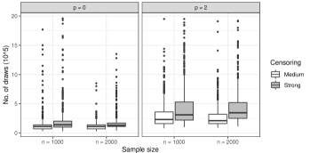
We compared MCMC convergence across the simulation conditions (Figure 3). Without covariates ($p=0$), convergence was obtained in less than $2.5\times 10^{5}$ draws in most replications. With covariates ($p=2$), more draws were needed, where the data sets exhibiting strong censoring required most draws. Still, at most $10^{6}$ draws were sufficient to achieve convergence in most cases in the $p=2$ setting. We also studied the rate of convergence by model parameters and found that the parameters of $f_{t}$ had slower convergence than those of $f_{x}$; see Supplementary Material, Section C.

Figure 3: Number of MCMC draws required to obtain Gelman-Rubin convergence statistic $R<1.1$ and an effective sample size of at least 30 for all parameters. 500 replicated data sets. Convergence evaluated every $10^{4}$ draws.

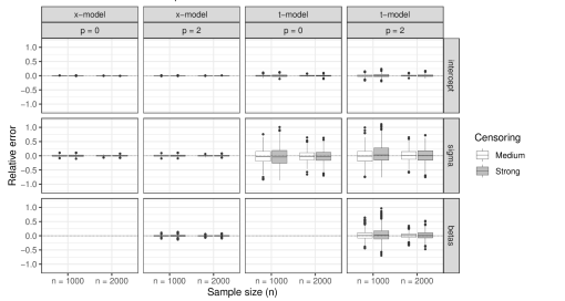
We compared the relative error of the parameter estimates of the Bayesian Gibbs sampler to those of ML-EM. Relative error was defined as $[\hat{\kappa}-\kappa]/\kappa$ where $\kappa$ is the true value of the parameter and $\hat{\kappa}$ a posterior median estimate or a ML estimate. Importantly, the performance characteristics of the Bayesian and the ML-EM estimators were equivalent. Figure 4 shows the relative errors of Bayes across the simulated replications; comparisons with ML-EM are given in the Supplemental Material, Section C. All parameters of $f_{x}$ and $f_{t}$ had approximately zero error in central tendency (i.e., the estimators were approximately unbiased). The estimates of the parameters of $f_{x}$ were more precise than the estimates of the parameters of $f_{t}$, where strong right censoring and introducing covariates ($p=2$) increased the variance of all parameter estimates. Estimates of $\sigma_{t}$ had higher variance than those of $\beta_{0,t}$ and $\beta_{1,t},\beta_{2,t}$. Precision increased with sample size, as can be seen by slightly narrower inter-quartile ranges in the $n=2000$ conditions (in addition, mean squared error estimates are given in the Supplemental Material, Section C). We also studied the estimated frequentist coverage probability of the 95% credible intervals which was at approximately nominal level for all parameters; see the Supplemental Material.

Figure 4: Relative error of Bayesian estimation compared to ML-EM for the parameters of the model for $t_{i}$ across 500 replications. Results for the parameters $\beta_{1}$ and $\beta_{2}$ are reported jointly as ’betas’.

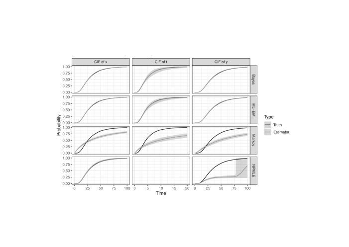
Bayesian estimation and ML-EM were compared with two existing methods: a progressive three-state constant hazard Markov model, implemented by R package msm (Jackson, 2011), and the NPMLE, implemented by package interval (Fay and Shaw, 2010). Figure 5 shows estimated marginal cumulative incidence functions (21) averaged point-wise over the replications for the setting with $p=2$, $n=1000$, and strong censoring (see Supplental Material, Section C, for all other conditions). The Markov model had a strong bias for all transition times, while the NPMLE approximated the CIF of $x_{i}$ correctly and failed for $y_{i}$. These results are plausible, as the Markov model assumes exponentially distributed transition times while the true distributions were lognormal. Furthermore, the NPMLE introduces informed censoring when estimating the CIF of $y_{i}$ (see Section 2). To the contrary, our Bayesian and ML-EM estimation methods yielded approximately unbiased CIF estimates. These results were similar under the other simulation conditions.

Finally, we evaluated whether the information criteria WAIC-1, WAIC-2, and DIC could select the correct model among various misspecified models; see the Supplemental Matierial, Section C. In particular, we misspecified the true model with lognormal $x_{i}$ and lognormal $t_{i}$ as either lognormal-Weibull, lognormal-exponential, Weibull-lognormal or Weibull-Weibull. The true distribution of $x_{i}$ was reliably selected, while the true distribution of $t_{i}$ was selected in 66% to 69% of runs correctly (with Weibull selected in the remainder), unless the sample size was $n=1000$ and censoring was strong (50%). However, even in the models using the Weibull for $t_{i}$ (or $x_{i}$), the regression coefficients and the CIFs were still estimated with negligible bias.

Figure 5: Marginal cumulative incidence functions (CIFs) compared for Bayesian estimation, ML-EM, the three-state Markov model, and the NPMLE. CIFs are point-wise averaged over 500 replications in the setting with $p=2$, $n=1000$, and strong censoring; for other conditions see Supplemental Material, Section C. 95% simulation intervals shown.

6 Application to POBASCAM data

POBASCAM was a randomized trial based on a random sample of 44,102 women from the Dutch population recruited in the time between 1999 and 2002. The trial compared a new screening protocol for CIN lesions to standard of care. The new protocol required patients to be screened earlier in time for CIN progression after an initial HPV diagnosis. As an important result, CIN-3 lesions were found earlier in women screened by the new protocol than by standard of care. In this study, we re-analyzed a subset of $n=1,454$ women from POBASCAM who were diagnosed as HPV-positive without cytological abnormalities at the start of trial (baseline). These women are considered a high-risk group for progression to CIN-2 and CIN-3. Our first objective was to estimate the distribution of the onset time from baseline until development of a CIN-2 lesion ($x_{i}$), the progression time from CIN-2 to CIN-3 ($t_{i}$), as well as the total transition time ($y_{i}=x_{i}+t_{i}$). Our second objective was identifying population heterogeneity by regressing the transition times on patient characteristics ($\operatorname{\mathbf{z}}_{i}$).

Women were followed for a maximum of 14.3 years (Table 3). The mean time to right censoring was 8.6 years. A total of 96 women (6.6%) were diagnosed with CIN-2; 176 women (12.1%) were diagnosed with CIN-3. Of the 176 women, 17 women had also developed a cancer. For this reason, we refer to the CIN-3 category as CIN-3+ in the following. CIN-2 and CIN-3+ lesions were found at screening times averaging 4.9 and 5.3 years, respectively. Patients had a mean age of 38.1 years at baseline. About half (52.7%) of women were diagnosed with a virus sub-type HPV-16, HPV-18 or HPV-31 which are associated with faster progression.

Table 3: Description of the analysis set of HPV-positive women from POBASCAM. Categories indicate the state at the time of censoring (HPV-positive, CIN-2 or CIN-3+)

	Total ($n=1,454$)	HPV-pos. ($n=1,182$)	CIN-2 ($n=96$)	CIN-3+ ($n=176$)
% of total	100	81.3	6.6	12.1
Max. screening time (years)	14.3	14.3	13.9	12.4
Time to censoring (mean/sd)	8.0 (3.0)	8.6 (2.6)	4.9 (3.5)	5.3 (2.9)
Age (mean/sd)	38.1 (8.5)	38.7 (8.7)	35.2 (6.8)	35.8 (6.9)
HPV-16 (%)	28.0	23.9	32.3	53.4
HPV-18 (%)	9.1	8.5	11.5	11.4
HPV-31 (%)	15.6	14.9	19.8	18.2

6.1 Implementation and analysis

We modeled (1-2), i.e., the log of the transition times from baseline to CIN-2 ($x_{i}$) and from CIN-2 to CIN-3+ ($t_{i}$), as linear combinations of patient age (z-standardized) and the HPV sub-type indicators (Table 3). The HPV sub-types are known causes of faster progression to CIN-3 and we assume that after including them as covariates, the conditional independence assumption discussed in Section 3, holds. In addition, a sensitivity analysis was conducted; see Section 6.4. We specified the error distributions of the AFT model (1-2) as either extreme value with $\sigma$ constrained to 1, extreme value (with $\sigma$ free), logistic, or normal, so that $x_{i}$ and $t_{i}$ were exponentially, Weibull, loglogistically or lognormally distributed (Table 1). We fitted all possible combinations, leading to $4\times 4=16$ models and subsequently performed model selection; see Section 4.3. We ran the Gibbs sampler (9-11) with fifteen randomly initialized MCMC chains and continued sampling until $R<1.1$ and the effective sample size was at least 1,000 for all parameters, dropping the first half of the draws. The MCMC chains were inspected for convergence.

6.2 Results

The lognormal-loglogistic model fitted the data best (i.e., the model using the lognormal for $x_{i}$ and the loglogistic for $t_{i}$), but models that used either a loglogistic or lognormal distribution for one of the transition times had almost identical fit (Table 4). Models involving the Weibull distribution for any transition time fitted slightly worse and models involving the exponential distribution had substantially worse fit. Model convergence was reached, depending on the model, between 4 and $11\times 10^{5}$ MCMC draws.

Table 4: Information criteria ordered by WAIC-1 and the total number of MCMC draws until convergence (first half dropped for warm-up). Reading example: lognormal-loglog is the model with lognormal $x_{i}$ and loglogistic $t_{i}$. All statistics were computed using $10^{5}$ posterior draws

Model	WAIC-1	WAIC-2	DIC	Draws ($\times 10^{5}$)
lognormal-loglogistic	1979.1	1979.4	1979.3	8
lognormal-lognormal	1979.6	1979.9	1979.7	7
loglogistic-loglogistic	1980.8	1981.1	1980.9	6
loglogistic-lognormal	1980.9	1981.2	1981.0	6
lognormal-Weibull	1981.2	1981.6	1981.2	7
loglogistic-Weibull	1982.6	1983.0	1982.6	6
Weibull-loglogistic	1983.2	1983.4	1983.3	8
Weibull-lognormal	1983.2	1983.5	1983.3	7
Weibull-Weibull	1985.2	1985.5	1985.2	7
loglogistic-exponential	2016.8	2017.3	2015.3	5
lognormal-exponential	2016.9	2017.4	2015.3	5
Weibull-exponential	2018.4	2018.9	2017.0	8
exponential-loglogistic	2154.8	2155.1	2154.3	11
exponential-lognormal	2154.9	2155.2	2154.4	8
exponential-Weibull	2156.7	2157.0	2156.0	8
exponential-exponential	2175.1	2175.5	2173.5	4

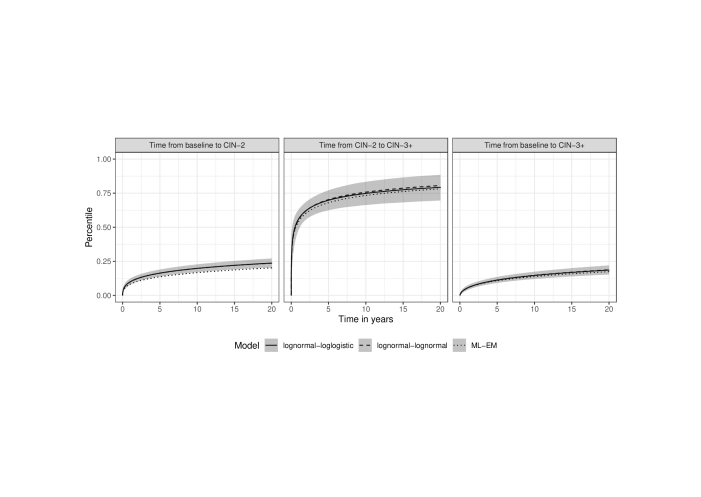
We compared the marginal predictive CIFs (21) of the lognormal-loglogistic model to the NPMLE, the progressive three-state Markov model, and the exponential-exponential model (Figure 6). The exponential-exponential model had worst fit (Table 4) and had similar CIFs as the Markov model. This result was expected, because the Markov model also assumes exponentially distributed transition times. However, the CIFs of both models deviated strongly from those of the lognormal-loglogistic model. In particular, the lognormal-loglogistic model CIFs had long tails suggesting that a part of the population never progresses from baseline to CIN-2 or from CIN-2 to CIN-3+ in their lifetime. The CIFs obtained by the NPMLE were similar to those of the lognormal-loglogistic model on the time from baseline to CIN-2 ($x_{i}$) up until the last observed screening time (14.3 years). Beyond this time point the estimator became imprecise. This result can be viewed as a validation of model fit, as the NPMLE is unbiased for this transition (Sections 2 and 5). Surprisingly, the CIF of $y_{i}$ was also close to the Bayesian fit, which was unexpected, as the NPMLE is biased for this transition. We suspect that the bias of the NPMLE was mitigated as the proportion of CIN-2 events was small (6.6%).

Based on the lognormal-loglogistic model, we estimated the probability for HPV-positive women to develop a CIN-2 lesion in the first twenty years after diagnosis of their HPV infection at 23.7% (95% credible interval (CI): [20.5, 27.2]; left plot, Figure 6). Progression from CIN-2 to CIN-3+ was much more rapid (middle plot); probability of progression within the first ten years after development of CIN-2 was 74.8% (95% CI: [66.2, 83.3]). Also, already at the end of the first year women had over 50% chance to have progressed. The time from baseline to CIN-3+ is the convolution of these two processes (right plot). CIN-3+ progression probability from baseline within the first twenty years was 18.6% (95% CI: [15.3, 22.0]).

Figure 6: Posterior median of predictive CIFs (21) for the Bayesian lognormal-loglogistic model (best performance acc. to all three information criteria) and the exponential-exponential model (worst performance) giving the cumulative probability to progress until a point in time. CIFs from a progressive three-state Markov model and the NPMLE are superimposed. 95% credible intervals of the lognormal-loglogistic model shown as dark shaded region. Bootstrapped 95% confidence intervals of the NPMLE shown as gray shaded region.

Table 5: Percentiles of the posterior distribution of the lognormal-loglogistic model
($x_{i}$: time to CIN-2; $t_{i}$: time from CIN-2 to CIN-3+)

	Model for $\log x_{i}$				Model for $\log t_{i}$
Parameter	$p_{.025}$	$p_{.50}$	$p_{.975}$		$p_{.025}$	$p_{.50}$	$p_{.975}$
Intercept	6.82	7.94	9.09		-1.31	-0.02	0.78
Age (standardized)	0.41	0.83	1.23		-1.23	-0.34	0.34
HPV-16*	-4.09	-3.04	-2.29		-4.45	-2.12	-1.01
HPV-18*	-2.68	-1.40	-0.44		-2.19	-0.47	0.77
HPV-31*	-2.48	-1.37	-0.56		-1.83	-0.33	0.80
sigma	4.09	4.96	5.85		1.55	2.71	4.58
* Reference: other HPV sub-type

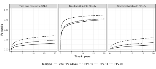
Table 5 displays posterior median parameter estimates for the parameters in (1-2) as well as 95% credible intervals (CI). Age had a positive effect and the three HPV sub-types had negative effects on the log-time from baseline to CIN-2 ($\log x_{i}$), where HPV-16 had the strongest effect ($\beta=-3.04$). Among the factors contributing to progression from CIN-2 to CIN-3+ ($\log t_{i}$) we, again, identified HPV-16 as the dominating factor ($\beta=-2.12$). There was no evidence for an influence of the other covariates. The effect of the HPV sub-types at a mean age (38.1 years) is illustrated by separate conditional predictive CIFs (20) in Figure 7. For example, women with HPV-16 sub-type had 30.0% risk of progression to CIN-3+ within 20 years (95% CI: [24.8, 35.5]), whereas women with types 18, 31, or a different subtype (’other’) had 18.0%, 17.6% and 11.5% risk, respectively. Similarly, progression from CIN-2 to CIN-3+ was faster for HPV-16 than for all other HPV sub-types; for example, 10-year progression risk was 84.2% for HPV-16 (95% CI: [74.6, 91.8]) and 70.5% for ’other’ types (95% CI: [61.2, 80.1]).

Figure 7: Posterior median of conditional predictive cumulative incidence functions (20) indicating the cumulative probability to progress until a point in time, given HPV sub-type and a mean age of 38.1 years (lognormal-loglogistic model).

6.3 Model fit by ML-EM

Estimation of the lognormal-lognormal model by ML-EM (Section 4.2) is discussed in detail in the Supplemental Material, Section D. We used $2\times 10^{4}$ importance samples in the numerical integration of the E-step and a convergence limit of $10^{-5}$. The maximum of the likelihood was determined by starting one hundred EM runs with random initialization. These runs converged at similar likelihood values but yielded quite different estimates of $\sigma_{t}$ and $\operatorname{\bm{\beta}}_{t}$ which was indicative of a flat and/or multi-modal likelihood function. The maximum likelihood estimates (i.e., the estimates from the run maximizing the likelihood across all runs) were similar to the posterior median estimates from the Bayesian lognormal-lognormal model. The CIFs matched those of the Bayesian model closely.

6.4 Conditional independence sensitivity analysis

We assessed the sensitivity of our findings to the conditional independence assumption of model (1-2), as described in Section 4.5, for the lognormal-loglogistic model. In particular, we specified a grid of parameters

$$(\beta_{x,w},\beta_{t,w})=\{(-3,3),(-2,2),(-1,1),(0,0),(1,1),(2,2),(3,3)\}$$

in model (22-23), where $(0,0)$ denotes the conditional independence model (1-2). The results of this analysis are shown in the Supplemental Material, Section D. The deviations from conditional independence caused a stronger curvature in the predictive CIFs, especially those of $t_{i}$. However, the conclusions of the main analysis did not change. Also the sign and significance of the regression coefficients did not change as compared to conditional independence.

6.5 Prior sensitivity analysis

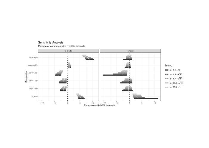
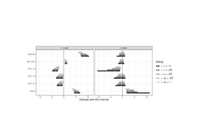
We assessed the sensitivity of the findings to alternative specifications of the weakly informative priors in the lognormal-loglogistic model. In particular, we considered two different t-distributions for $\beta$: $student(\tau=1)$ and $student(\tau=30)$, as opposed to $student(\tau=4)$ in our main analysis. These choices denote the central Cauchy and an approximate standard-normal distribution, respectively. For $student(\tau=30)$ we expect stronger regularization due to flat tails, whereas $student(\tau=1)$ has substantially wider tails than $student(\tau=4)$. Furthermore, the main analysis assumed a half-normal $N(0,\lambda=\sqrt{10})$ prior for $\sigma_{x}$ and $\sigma_{t}$. As alternatives, we considered $\lambda=1$ and $\lambda=10$ which are more and less restrictive, respectively. The predictive CIFs of $x_{i}$ and $y_{i}$ were insensitive to the prior alternatives (Figure 8). Furthermore, also the predictive CIF of $t_{i}$ was not sensitive to changes in $\tau$, but exhibited moderate sensitivity to $\lambda$. The influence of the choice of $\tau$ on the posterior distributions of the parameters was negligible, although $\tau=30$ caused slightly stronger shrinkage, as expected (Figure 9). However, $\lambda$ had a more profound impact: the posterior variance of $\sigma_{t}$ and $\beta_{t}$ of HPV-16 increased strongly under $\lambda=10$, illustrating the benefits of regularizing the parameters more strongly by setting $\lambda=\sqrt{10}$.

Figure 8: Posterior median of predictive cumulative incidence functions (21) for different weakly informative hyperparameter choices. The main analysis model uses $\tau=4$, $\lambda=\sqrt{10}$ (lognormal-loglogistic)).

Figure 9: Posterior parameter sensitivity to different weakly informative hyperparameter choices. The main analysis model uses $\tau=4$, $\lambda=\sqrt{10}$ (lognormal-loglogistic).

7 Discussion

The screening data considered in the present study have a very specific censoring structure (Figure 1): if state 2 of a disease or a condition is found at a screening time, the condition is treated (e.g., a CIN-2 lesion is surgically removed). As a result, the progression time ($t_{i}$) to state 3 remains unobserved. It is bounded only by the most recent screening interval if the patient progresses to, both, states 2 and 3, in the same interval. This data structure was present in the POBASCAM trial from the screening of HPV-positive women. However, there are many more health conditions where screening programs yield similar data; examples are colon cancer (e.g., with states adenoma and cancer) and breast cancer (e.g., with states ductal carcinoma in situ and cancer). In both cases, screening and prevention programs are in place to timely detect and treat the onset condition (state 2). The proposed three-state model, therefore, is anticipated to have wider applicability.

To estimate the model, we suggested a Bayesian Gibbs sampler (Section 4.1) and we also considered using a frequentist estimator (Section 4.2) that finds the maximum of the likelihood by an expectation-maximization algorithm (ML-EM). In simulations, both estimators had similarly good performances. However, Bayesian estimation, in our view, is the preferable approach for three reasons. First, the Bayesian data augmentation scheme (10-11) allows fitting flexible AFT models for arbitrary transition time distributions including models for non-constant and non-proportional hazards. ML-EM requires specific implementations for any combination of distributions, where we focused on the lognormal-lognormal model. Second, Bayesian estimation enables posterior inference for parameters and CIFs, while ML-EM has to rely on re-sampling techniques. The Bayesian credible intervals were shown to have good frequentist performance. Third, while the approaches had similar performance in the simulation study, ML-EM suffered from convergence problems in the application to the POBASCAM data. Across repeated randomly initialized runs, the algorithm converged at similar likelihood values that, however, yielded different estimates for the parameters of $f_{t}$ indicating that the likelihood function was almost flat and/or multi-modal. When the likelihood is almost flat, the convergence of the EM algorithm at maximum likelihood estimates generally hinges on setting the convergence limit to a small enough value while making sure that the numerical integration in the E-step is sufficiently precise. Hence, the procedure can become computationally very expensive. The Bayesian answer to these problems is to apply regularized parameter estimation by including weak prior information. This measure strongly improved estimation performance, in that a single random initialization of multiple MCMC chains converged to the posterior distribution. However, we emphasize that the suggested weakly informative priors are important for the performance of the Gibbs sampler and that the priors should not, in general, be chosen non-informative (i.e., flat). This is indicated by the prior sensitivity analysis (Figure 9) demonstrating that the less informative prior choice ($\lambda_{t}=10$) inflated the posterior variance. A non-informative prior (large $\lambda$) would likely further increase this variance implying slower convergence and less robust estimates.

We compared Bayesian estimation also to a three-state Markov model and a NPMLE, which are convenient choices for practitioners but can have bias. The NPMLE can be used to estimate the CIF of $x_{i}$ but cannot be used for $y_{i}$ (Sections 2 and 5). Furthermore, Markov models can be easily fit to a wide range of transition and censoring structures under a constant hazards assumption (Jackson, 2011). However, in many applications hazards change over time. HPV infections can clear, for example, so that hazards decrease. This leads to CIFs approaching a ceiling value below one, where non-progressed cases subsumed in the tail are not expected to progress within relevant time frames (e.g., 20 or 30 years). Markov models lack the flexibility to fit such transitions (Figures 5 and 6). The estimated transition probabilities by our model, still, depend on a correct model specification and also have to be judged in the context of the maximum follow-up (14.3 years). Within these constraints, we predicted that about 24% and 19% of women progress to, respectively, CIN-2 and CIN-3+ within 20 years after their HPV diagnosis. Progression from CIN-2 to CIN-3+ is rapid: more than half of women progress within a year and about 75% of women progress within 10 years. The remaining women have low probability to progress in their lifetime. Our model also allows including covariates to uncover population heterogeneity. We found that women with HPV-16, -18, and -31 sub-types had a strongly decreased transition time, where the effect of HPV-16 was strongest. Also, younger women showed faster progression to CIN-2. Determining an optimal screening schedule for different screening sub-groups is an important topic for further research. For example, the posterior samples of transition times from our model may be used in simulations that compare different screening schedules.

The latent Continuous-Time Markov Chains model (CTMC) implemented in R package cthmm by Lange and Minin (2013) and the piece-wise constant hazard model in package msm (Jackson, 2011) can be viewed as alternative modeling approaches. The methods make approximations of non-constant hazards under proportional hazard assumptions. Their accuracy hinges on the appropriateness of this assumption and good choices of latent transition structures or knots, respectively, which can require expert knowledge for successful implementations. Users of the proposed Bayesian method do not need to make similar decisions. However, our method makes several assumptions whose appropriateness has to be judged in each application. First, the transition and censoring structure (4-5) has to be appropriate. Second, the AFT specification (1-2) assumes independent errors conditionally on the covariates. In our study, the most important cause of faster transition, HPV sub-type, was included and a sensitivity analysis was conducted. Third, the error distributions need to be correctly specified and the information criteria (e.g., WAIC) allow model selection. However, our simulation indicated that even misspecified semi-Markov transitions (e.g., Weibull for a true lognormal transition) only cause minor bias on the parameter estimates and CIFs. In addition, the NPMLE for $x_{i}$ can be used as an indication of goodness of fit. Fourth, we assumed non-informative interval censoring in the sense that the transition times $x_{i}$ and $t_{i}$ are independent of the screening times conditionally on covariates. This means that within strata defined by age groups and HPV sub-types the screening visits were not patient initiated due to symptomatic disease states. In POBASCAM, this assumption was plausible as CIN-2/3 lesions are asymptomatic and screening schedules were planned in advance. Fifth, we assumed that the disease state of a patient can be ascertained without error. In POBASCAM, women were screened by cytology combined with PCR-DNA test which has high accuracy or by cytology alone having moderate accuracy. However, the effect of ignoring the imperfect sensitivity on the estimated incidence functions is expected to be limited (Witte et al., 2017). Still, extending the Bayesian model to allow for patient initiated screening times and misclassified states are viable paths for further research.

References

- Albert and Chib (1993) James H Albert and Siddhartha Chib. Bayesian analysis of binary and polychotomous response data. J Am Stat Assoc, 88(422):669–679, 1993.
- Asanjarani et al. (2021) Azam Asanjarani, Benoit Liquet, and Yoni Nazarathy. Estimation of semi-markov multi-state models: a comparison of the sojourn times and transition intensities approaches. Int J Biostat, 2021.
- Boruvka and Cook (2016) Audrey Boruvka and Richard J Cook. Sieve estimation in a markov illness-death process under dual censoring. Biostatistics, 17(2):350–363, 2016.
- De Gruttola and Lagakos (1989) Victor De Gruttola and Stephen W Lagakos. Analysis of doubly-censored survival data, with application to aids. Biometrics, pages 1–11, 1989.
- de Wreede et al. (2011) Liesbeth C de Wreede, Marta Fiocco, and Hein Putter. mstate: an r package for the analysis of competing risks and multi-state models. J Stat Softw, 38(1):1–30, 2011.
- Dijkstra et al. (2016) Maaike G Dijkstra, Marjolein van Zummeren, Lawrence Rozendaal, Folkert J van Kemenade, Theo JM Helmerhorst, Peter JF Snijders, Chris JLM Meijer, and Johannes Berkhof. Safety of extending screening intervals beyond five years in cervical screening programmes with testing for high risk human papillomavirus: 14 year follow-up of population based randomised cohort in the netherlands. Bmj, 355, 2016.
- Fay and Shaw (2010) Michael P Fay and Pamela A Shaw. Exact and asymptotic weighted logrank tests for interval censored data: the interval r package. J Stat Softw, 36(2), 2010.
- Foucher et al. (2007) Yohann Foucher, Magali Giral, Jean-Paul Soulillou, and Jean-Pierre Daures. A semi-markov model for multistate and interval-censored data with multiple terminal events. application in renal transplantation. Stat Med, 26(30):5381–5393, 2007.
- Foucher et al. (2010) Yohann Foucher, M Giral, JP Soulillou, and JP Daures. A flexible semi-markov model for interval-censored data and goodness-of-fit testing. Stat Methods Med Res, 19(2):127–145, 2010.
- Gelman et al. (1995) Andrew Gelman, John B Carlin, Hal S Stern, and Donald B Rubin. Bayesian data analysis. Chapman and Hall/CRC, 1995.
- Gelman et al. (2008) Andrew Gelman, Aleks Jakulin, Maria Grazia Pittau, and Yu-Sung Su. A weakly informative default prior distribution for logistic and other regression models. Ann Appl Stat, 2(4):1360–1383, 2008.
- Gelman et al. (2014) Andrew Gelman, Jessica Hwang, and Aki Vehtari. Understanding predictive information criteria for bayesian models. Stat Comput, 24(6):997–1016, 2014.
- Jackson (2011) Christopher Jackson. Multi-state models for panel data: the msm package for r. J Stat Softw, 38(1):1–28, 2011.
- Jackson (2016) Christopher H Jackson. flexsurv: a platform for parametric survival modeling in r. J Stat Softw, 70, 2016.
- Kang and Lagakos (2007) Minhee Kang and Stephen W Lagakos. Statistical methods for panel data from a semi-markov process, with application to hpv. Biostatistics, 8(2):252–264, 2007.
- Komárek and Lesaffre (2008) Arnošt Komárek and Emmanuel Lesaffre. Bayesian accelerated failure time model with multivariate doubly interval-censored data and flexible distributional assumptions. J Am Stat Assoc, 103(482):523–533, 2008.
- Lange and Minin (2013) Jane M Lange and Vladimir N Minin. Fitting and interpreting continuous-time latent markov models for panel data. Stat Med, 32(26):4581–4595, 2013.
- Lange et al. (2018) Jane M Lange, Roman Gulati, Amy S Leonardson, Daniel W Lin, Lisa F Newcomb, Bruce J Trock, H Ballentine Carter, Matthew R Cooperberg, Janet E Cowan, Lawrence H Klotz, et al. Estimating and comparing cancer progression risks under varying surveillance protocols. Ann Appl Stat, 12(3):1773, 2018.
- Mandel (2010) Micha Mandel. Estimating disease progression using panel data. Biostatistics, 11(2):304–316, 2010.
- Rijkaart et al. (2012) Dorien C Rijkaart, Johannes Berkhof, Lawrence Rozendaal, Folkert J van Kemenade, Nicole WJ Bulkmans, Daniëlle AM Heideman, Gemma G Kenter, Jack Cuzick, Peter JF Snijders, and Chris JLM Meijer. Human papillomavirus testing for the detection of high-grade cervical intraepithelial neoplasia and cancer: final results of the pobascam randomised controlled trial. Lancet Oncol, 13(1):78–88, 2012.
- Titman and Sharples (2010) Andrew C Titman and Linda D Sharples. Semi-markov models with phase-type sojourn distributions. Biometrics, 66(3):742–752, 2010.
- Turnbull (1976) Bruce W Turnbull. The empirical distribution function with arbitrarily grouped, censored and truncated data. J R Stat Soc Series B Stat Methodol, 38(3):290–295, 1976.
- Wei and Kryscio (2016) Shaoceng Wei and Richard J Kryscio. Semi-markov models for interval censored transient cognitive states with back transitions and a competing risk. Stat Methods Med Res, 25(6):2909–2924, 2016.
- Witte et al. (2017) Birgit I Witte, Johannes Berkhof, and Marianne A Jonker. An em algorithm for nonparametric estimation of the cumulative incidence function from repeated imperfect test results. Stat Med, 36(21):3412–3421, 2017.