Learning Sparse Masks for
Diffusion-based Image Inpainting

Abstract

Diffusion-based inpainting is a powerful tool for the reconstruction of images from sparse data. Its quality strongly depends on the choice of known data. Optimising their spatial location – the inpainting mask – is challenging. A commonly used tool for this task are stochastic optimisation strategies. However, they are slow as they compute multiple inpainting results. We provide a remedy in terms of a learned mask generation model. By emulating the complete inpainting pipeline with two networks for mask generation and neural surrogate inpainting, we obtain a model for highly efficient adaptive mask generation. Experiments indicate that our model can achieve competitive quality with an acceleration by as much as four orders of magnitude. Our findings serve as a basis for making diffusion-based inpainting more attractive for applications such as image compression, where fast encoding is highly desirable.

1 Introduction

Inpainting is the task of restoring an image from limited amounts of data. Diffusion processes are particularly powerful for reconstructions from sparse data; see e.g. [32]. By solving a partial differential equation (PDE), they propagate information from a small known subset of pixels, the inpainting mask, to the missing image areas. Inpainting from sparse data is successful in applications such as image compression [13, 27, 29], adaptive sampling [9], and denoising [1].

Optimising the inpainting mask is essential for a good reconstruction. However, this is a challenging combinatorial problem. While there are theoretical results on optimal masks [5], practical implementations are often qualitatively not that convincing albeit highly efficient. On the other hand, stochastic mask optimisation strategies [15, 22] produce high quality masks, but are computationally expensive.

In the present paper, we combine efficiency and quality of mask optimisation for PDE-based inpainting with the help of deep learning. To this end, we design a hybrid architecture which, to the best of our knowledge, constitutes the first instance of learned sparse masks for PDE-based inpainting.

1.0.1 Our Contribution.

We present a model for learning sparse inpainting masks for homogeneous diffusion inpainting. This type of inpainting shows good performance for optimised masks [22], and does not depend on any free parameters. We employ two networks: one which generates a sparse inpainting mask, and one which acts as a surrogate solver for homogeneous diffusion inpainting. By using different loss functions for the two networks, we optimise both inpainting quality and fidelity to the inpainting equation.

The use of a surrogate solver is a crucial novelty in our work. It reproduces results of a diffusion-based inpainting process without having to perform backpropagation through iterations of a numerical solver. This replicates the full inpainting pipeline to efficiently train a mask optimisation model.

We then evaluate the quality of the learned masks in a learning-free inpainting setting. Our model combines the speed of instantaneous mask generation approaches [5] with the quality of stochastic optimisation [22]. Thus, we reach a new level in sparse mask optimisation for diffusion-based inpainting.

1.0.2 Related Work.

Diffusion-based inpainting plays a vital role in image and video compression [3, 13, 29], denoising [1], and many more. A good inpainting mask is crucial for successful image inpainting. Current approaches for the spatial optimisation of sparse inpainting data in images can be classified in four categories.

1. Analytic Approaches. Belhachmi et al. [5] have shown that in the continuous setting, optimal masks for homogeneous diffusion inpainting can be obtained from the Laplacian magnitude of the image. In practice this strategy is very fast, allowing real-time inpainting mask generation by dithering the Laplacian magnitude. However, the reconstruction quality is lacking, mainly due to limitations in the quality of the dithering operators [15, 22].

2. Nonsmooth Optimisation Strategies. Several works [6, 7, 15, 25] consider sophisticated nonsmooth optimisation approaches that offer high quality, but do not allow to specify the desired mask density in advance. Instead one influences it by varying a regularisation parameter, which requires multiple program runs, resulting in a slow runtime. Moreover, adapting the model to different inpainting approaches is not trivial.

3. Sparsification Methods. They successively remove pixel data from the image to create an adaptive inpainting mask. For example, the probabilistic sparsification (PS) of Mainberger et al. [22] randomly removes a set of points and reintroduces a fraction of those points with a high inpainting error. Sparsification strategies are generic as they work with various inpainting operators such as diffusion-based ones [15, 22] or interpolation on triangulations [11, 23]. Moreover, they allow to specify the desired mask density in advance. However, they are also computationally expensive as they require many inpaintings to judge the importance of individual data points to the reconstruction. Due to their simplicity and their broad applicability, sparsification approaches are the most widely used mask optimisation strategies.

4. Densification Approaches. Densification strategies [8, 10, 19] start with empty or very sparse masks and successively populate them. This makes them reasonably efficient, while also yielding good quality. They are fairly easy to implement and work well for PDE-based [8, 10] and exemplar-based [19] inpainting operators. Still, they require multiple inpainting steps in the range of 10 to 100 to obtain a sufficiently good inpainting mask.

In order to escape from suboptimal local minima, the Categories 3 and 4 have been improved by nonlocal pixel exchange (NLPE) [22], at the expense of additional inpaintings and runtime. Moreover, it is well-known that optimising the grey or colour values of the mask pixels – so-called tonal optimisation – can boost the quality even further [15, 22]. Also the approaches of Category 2 may involve tonal optimisation implicitly or explicitly.

Qualitatively, carefully tuned approaches of Categories 2–4 play in a similar league, and are clearly ahead of Category 1. However, their runtime is also substantially larger than Category 1, mainly due to the many inpaintings that they require. Last but not least, all aforementioned approaches are fully model-based, in contrast to most recent approaches in image analysis that benefit from deep learning ideas.

The goal of the present paper is to show that the incorporation of deep learning can give us the best of two worlds: a real-time capability similar to Category 1, and a quality similar to Categories 2–4. In order to focus on the main ideas and to keep things simple, we restrict ourselves to homogeneous diffusion inpainting and compare only to probabilistic sparsification without and with NLPE. Also tonal optimisation is not considered in our paper, but is equally possible for our novel approach. More refined approaches and more comprehensive evaluations will be presented in our future work.

Learning-based inpainting has also been successful in recent years. Following the popular work of Xie et al. [33], several architectures and strategies for inpainting have been proposed; see e.g. [18, 21, 26, 34, 35]. However, inpainting from sparse data is rarely considered. Vašata et al. [31] present sparse inpainting based on Wasserstein generative adversarial networks. Similarly, Ulyanov et al. [30] consider inpainting from sparse data without mask generation. Dai et al. [9] present a trainable mask generation model from an adaptive sampling viewpoint. Our approach is the first to combine deep learning for mask optimisation for PDE-based inpainting in a transparent and efficient way.

1.0.3 Organisation of the Paper.

In Section 2, we briefly review diffusion-based inpainting. Afterwards in Section 3, we introduce our model for learning inpainting masks. We evaluate the quality of the learned masks in Section 4 before presenting our conclusions in Section 5.

2 Review: Diffusion-based Inpainting

The goal of inpainting is to restore missing information in a continuous greyscale image $f:\Omega\rightarrow\mathbb{R}$ on some rectangular domain $\Omega$, where image data is only available on an inpainting mask $K\subset\Omega$. In this work we focus on homogeneous diffusion inpainting, which computes the reconstruction $u$ as the solution of the PDE

$$\left(1-c\right)\Delta u-c\left(u-f\right)=0$$ (1)

with reflecting boundary conditions. Here, a confidence measure $c:\Omega\rightarrow\mathbb{R}$ denotes whether a value is known or not. Most diffusion-based inpainting models consider binary values for $c$: A value of $c(\bm{x})=1$ indicates known data and thus $u=f$ on $K$, while $c(\bm{x})=0$ denotes missing data, leading to homogeneous diffusion [17] inpainting $\Delta u=0$ on $\Omega\backslash K$, where $\Delta=\partial_{xx}+\partial_{yy}$ denotes the Laplacian. However, it is also possible to use non-binary confidence measures [16], which we will exploit to our advantage.

We consider digital greyscale images $\bm{u},\bm{f}\in\mathbb{R}^{n_{x}n_{y}}$ with dimensions $n_{x}\times n_{y}$ and discretise the inpainting equation (1) by means of finite differences. Then a numerical solver for the resulting linear system of equations is used to obtain a reconstruction $\bm{u}$. For a good inpainting quality, optimising the binary mask $\bm{c}\in\{0,1\}^{n_{x}n_{y}}$ is crucial. This problem is constrained by a desired mask density $d$ which measures the percentage of mask pixels w.r.t. the number of image pixels.

One strategy for mask optimisation has been proposed by Belhachmi et al. [5]. They show that an optimal mask in the continuous setting can be obtained from the rescaled Laplacian magnitude of the image. However, transferring these results to the discrete setting often suffers from suboptimal dithering strategies. While being highly efficient, reconstruction quality is not fully satisfying.

Better quality can be achieved with the popular stochastic strategies of Mainberger et al. [22]. First, one employs probabilistic sparsification (PS): Starting with a full mask, one removes a fraction $p$ of candidate pixels and computes the inpainting. Then one reintroduces a fraction $q$ of the candidates with the largest local inpainting error. One repeats this step until reaching a desired mask density $d$.

Since sparsification is a greedy local approach, it can get trapped in bad local minima. As a remedy, Mainberger et al. [22] also propose a nonlocal pixel exchange (NLPE). Pixel candidates in a sparsified mask are exchanged for an equally large set of non-mask pixels. If the new inpainting result improves, the exchange is kept, otherwise it is discarded. In theory, NLPE can only improve the mask, but in practice convergence is slow.

The use of PS and NLPE requires to solve the inpainting problem numerous times, leading to slow mask optimisation. To avoid this computational bottleneck, we want to reach the quality of stochastic mask optimisation with a more efficient model based on deep learning.

Figure 1: Overview over our model structure. Solid lines denote forward passes, dashed lines denote backpropagation.

3 Sparse Masks with Surrogate Inpainting

Our model consists of two equally shaped U-nets [28] with different loss functions. By optimising both inpainting quality and fidelity to the inpainting equation, we obtain masks with good reconstruction quality for the inpainting problem.

3.1 The Mask Network

The mask network takes an original image $\bm{f}$ and transforms it into a mask $\bm{c}$. We denote the forward pass through the mask network by $\mathcal{M}(\cdot)$, i.e. the mask is computed as $\bm{c}=\mathcal{M}(\bm{f})$.

The mask entries lie in the interval $\left[0,1\right]$. Permitting non-binary values allows for a differentiable network model. To obtain mask points in the desired range, we apply a sigmoid function to the output of the network. Moreover, the mask network is trained for a specific mask density $d$. To this end, we rescale the outputs of the network if they exceed the desired density. We do not require a lower bound, since the loss function incites a sufficiently dense mask.

The mask network places the known data such that the inpainting error between the reconstruction $\bm{u}$ and the original image $\bm{f}$ is minimised. This yields the inpainting loss

$$\mathcal{L}_{I}\!\left(\bm{u},\bm{f}\right)=\frac{1}{n_{x}n_{y}}\|\bm{u}-\bm{f}\|_{2}^{2}$$ (2)

as its objective function where $\|\cdot\|_{2}$ is the Euclidean norm. Its implicit dependency on the inpainting mask links the learned masks to the reconstructions.

We found that the mask network tends to get stuck in local minima with flat masks which are constant at every position, yielding a random sampling. To avoid this, we add a regularisation term $\mathcal{R}(\bm{c})$ to the inpainting loss $\mathcal{L}_{I}(\bm{u},\bm{f})$. It penalises the inverse variance of the mask via $\mathcal{R}(\bm{c})=\left(\sigma^{2}_{\bm{c}}+\epsilon\right)^{-1}$ where a small constant $\epsilon$ avoids division by zero. The variance of a mask describes how strongly the confidence measures of the individual pixels differ from the mean probability. Thus, the regulariser serves two purposes: First, it lifts the bad local minima for flat masks by adding a strong penalty to the energy. Second, it promotes probabilities closer to $0$ and $1$, as this maximises the variance. The impact of the regularisation term is steered by a positive regularisation parameter $\alpha$.

3.2 The Inpainting Network

The second network is called the inpainting network. Its task is to create a reconstruction $\bm{u}$ which follows a classical inpainting process. In [2], it has been shown that U-nets realise an efficient multigrid strategy at their core. Thus, we use a U-net as a surrogate solver which reproduces the results of the PDE-based inpainting. The inpainting network takes the original image $\bm{f}$ and the mask $\bm{c}$ and creates a reconstruction $\bm{u}=\mathcal{I}\left(\bm{f},\bm{c}\right)$. This result should solve the discrete version of the inpainting equation (1) which reads

$$\left(\bm{I}-\bm{C}\right)\bm{A}\bm{u}-\bm{C}\left(\bm{u}-\bm{f}\right)=0.$$ (3)

Here, $\bm{A}$ is a discrete implementation of the Laplacian $\Delta$ with reflecting boundary conditions, and $\bm{C}=\text{diag}(\bm{c})$ is a matrix representation of the mask. To ensure that the reconstruction $\bm{u}$ approximates a solution to this equation, we minimise its residual, yielding the residual loss

$$\mathcal{L}_{R}\!\left(\bm{u},\bm{f},\bm{c}\right)=\frac{1}{n_{x}n_{y}}\|\left(\bm{I}-\bm{C}\right)\bm{A}\bm{u}-\bm{C}\left(\bm{u}-\bm{f}\right)\|_{2}^{2}\,.$$ (4)

As the residual loss measures fidelity to the PDE-based process, an optimal network approximates the PDE solution in an efficient way that allows fast backpropagation. This strategy has been proposed in [2] and is closely related to the idea of deep energies [14].

Figure 1 presents an overview of the full model structure. Note that the inpainting network receives both the mask and the original image as an input. Thus, this network is not designed for standalone inpainting. However, this allows the network to easily minimise the residual loss by transforming the original into an accurate inpainting result, given the mask as side information.

3.3 Practical Application

After training the full pipeline in a joint fashion, the mask network can be used to generate masks for homogeneous diffusion inpainting. To this end, we apply the mask network to an original image and obtain a non-binary mask. This mask is then binarised: The probability of a pixel belonging to a mask is given by its non-binary value. At each position, we perform a weighted coin flip with that probability. Afterwards, the binarised masks are fed into a numerical solver of choice for homogeneous diffusion inpainting.

While binarising the mask is not necessary in this pure inpainting framework, it is important for compression applications since storing binary masks with arbitrary point distributions is already highly non-trivial [24].

boat	cameraman	house	trui	peppers

Figure 2: Test images of resolution $256\times 256$.

4 Experiments

4.1 Experimental Setup

We train both U-nets jointly with their respective loss function on the BSDS500 dataset [4] which contains a broad selection of natural images. As a training set, we use $200$ cropped grey value images of size $256\times 256$ with values in the range $[0,255]$. We do not use a validation set as the training process is fully fixed.

Both U-nets employ $5$ scales, with $3$ layers per scale. On the finest scale, they use $10$ channels, and this number is doubled on each scale. Thus, each U-net possesses around $9\times 10^{5}$ parameters. We use the Adam optimiser [20] with standard settings, a learning rate of $5\cdot 10^{-4}$, and $4000$ epochs. As a regularisation parameter we choose $\alpha=0.01$. We found this combination of hyperparameters to work well in practice. We train multiple instances of the model for densities between $10\%$ and $1\%$ with several random initialisations.

After training, we binarise the masks and use them with a conjugate gradient solver for homogeneous diffusion inpainting to obtain a reconstruction. Since we aim at the highest quality, we take the best result out of $30$ samplings.

original	Belhachmi et al.	PS + NLPE	our model

(a) peppers with $8\%$ density

original	Belhachmi et al.	PS + NLPE	our model

(b) trui with $5\%$ density

Figure 3: Visual comparison of inpainting results on two exemplary images for different mask densities. Mask points are shown in black, and mask images are framed for better visibility. Top rows depict the inpainting results, and bottom rows display the masks, respectively. The learned masks yield inpainting results which are visually comparable to PS with additional NLPE.

Analogously, we generate masks with PS as well as with PS with additional NLPE. In the following, we denote the latter combination by PS+NLPE. In our sparsification we use candidate fractions $p=0.1$ and $q=0.05$ as suggested by Mainberger et al. [22], and we take the best result out of $5$ runs. For NLPE, we use $30$ candidates of which $10$ are exchanged. We run NLPE for $10$ cycles: In a single cycle, each mask point is exchanged once on average. Moreover, we compare against the strategy of Belhachmi et al. [5]. This approach is realised by taking the Laplacian magnitude of the image, rescaling it to obtain a desired density, and dithering the result with a binary Floyd–Steinberg algorithm [12].

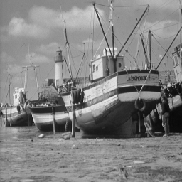
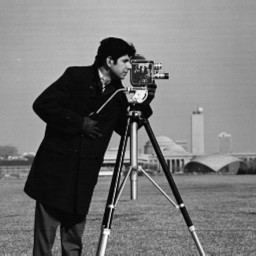
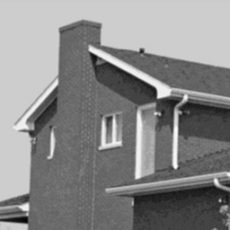
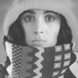
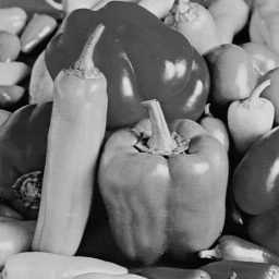
We compare our results on five popular test images (see Figure 2), since performing PS and NLPE on a large database is infeasible. We measure the quality in terms of peak signal-to-noise ratio (PSNR). Higher values indicate better quality.

Figure 4: Comparison of models in terms of quality and efficiency. (a) Left: Average inpainting quality in PSNR for each density. (b) Right: Efficiency in terms of the number of inpaintings for each density. The learned masks consistently outperform those of Belhachmi et al. and can compete with masks generated by PS. For very sparse masks, our model can compete with PS+NLPE. Both our method and that of Belhachmi et al. generate masks without computing an inpainting. The stochastic optimisation strategies compute up to thousands of inpaintings.

4.2 Reconstruction Quality

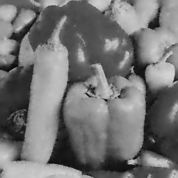
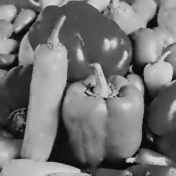
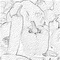
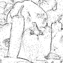
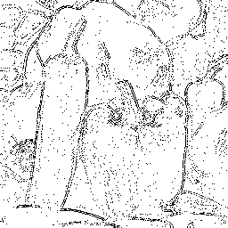
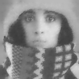
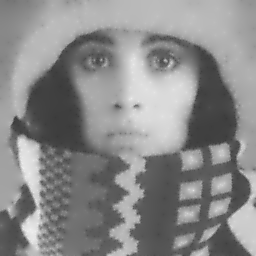
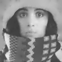
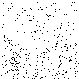
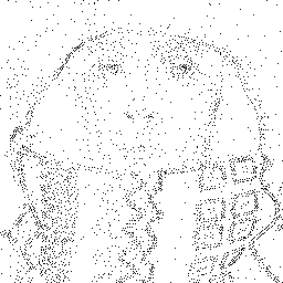
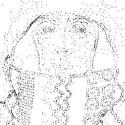
Figure 3 shows a visual comparison of optimised masks and the corresponding inpainting results. For both test cases, we observe that our learned masks are structurally similar to those obtained by PS with NLPE. This helps to create sharper contours, whereas the inpainting results of Belhachmi et al. suffer from fuzzy edges. The visual quality of the inpainting results for our model and PS+NLPE is indeed competitive.

Figure 4(a) presents a comparison of the reconstruction quality averaged over the test images. Our learned masks consequently outperform the strategy of Belhachmi et al.. Moreover, our model is on par with PS for densities smaller than $5\%$. For extremely small densities up to $2\%$, it even outperforms PS and is on par with PS+NLPE.

For larger mask densities, the margin between the methods becomes smaller, and our model cannot outperform its stochastic counterparts. Still, all models produce a good reconstruction quality. However, for applications such as inpainting-based image compression, very sparse masks are more important and more challenging [22, 29]. Therefore, our mask generation model performs well for the practically relevant mask densities.

4.3 Computational Efficiency

The decisive advantage of the learned mask generation is its speed. As inpainting operations are the dominant factor for computation time, we use the number of inpaintings as a measure for efficiency. In comparison, the forward pass of the mask network is negligible.

Figure 4(b) visualises the average number of inpaintings required to obtain masks of a specific density for the test set. To generate a mask, both our model and that of Belhachmi et al. do not require any inpainting operations. Thus, the efficiency of these mask generation strategies does not depend on the density.

For PS, lower densities require more inpainting operations. Adding NLPE requires even more inpaintings depending on the number of cycles and the mask density. Both strategies trade computational efficiency for inpainting quality.

For example, a single sparsification run for a $3\%$ mask on the cameraman image with realistic parameter settings requires $700$ steps. On an Intel Core i7-7700K CPU @ 4.20GHz, this amounts to $58$ seconds of runtime. The subsequent NLPE optimisation requires another $2000$ steps, resulting in more than $3$ minutes of additional runtime. In contrast, the strategy of Belhachmi et al. does not require any inpainting, and a mask can be generated in only $24$ milliseconds.

Our model requires only $85$ milliseconds for passing a single image through the mask network on the CPU. Thus, it plays in the same league as the strategy of Belhachmi et al., while being on par with the stochastic optimisation in terms of quality. This allows instantaneous high quality mask generation. As a consequence, our learned model can serve as a highly efficient replacement of stochastic mask optimisation.

5 Conclusions

We have proposed the first approach of sparse mask learning for diffusion-based inpainting. It fuses ideas from deep learning with classical homogeneous diffusion inpainting. The key of this strategy is a combination of an inpainting loss for the mask generator and a residual loss for the surrogate inpainting network. Its results are competitive with stochastic mask optimisation, while being up to four orders of magnitude faster. This constitutes a new milestone in mask optimisation for diffusion-based inpainting.

We are currently extending this idea to more sophisticated inpainting operators, as well as to further optimisations of the network architecture. We hope that this will pave the way to overcome the current time-consuming data optimisation strategies and will become an essential component for real-time diffusion-based codecs in hitherto unmatched quality.

References

- [1] Adam, R.D., Peter, P., Weickert, J.: Denoising by inpainting. In: Lauze, F., Dong, Y., Dahl, A.B. (eds.) Scale Space and Variational Methods in Computer Vision, Lecture Notes in Computer Science, vol. 10302, pp. 121–132. Springer, Cham (2017)
- [2] Alt, T., Schrader, K., Augustin, M., Peter, P., Weickert, J.: Connections between numerical algorithms for PDEs and neural networks. arXiv:2107.14742v1 [math.NA] (Jul 2021)
- [3] Andris, S., Peter, P., Mohideen, R.M.K., Weickert, J., Hoffmann, S.: Inpainting-based video compression in FullHD. In: Elmoataz, A., Fadili, J., Quéau, Y., Rabin, J., Simon, L. (eds.) Scale Space and Variational Methods in Computer Vision, Lecture Notes in Computer Science, vol. 12679, pp. 425–436. Springer, Cham (2021)
- [4] Arbelaez, P., Maire, M., Fowlkes, C., Malik, J.: Contour detection and hierarchical image segmentation. IEEE Transactions on Pattern Analysis and Machine Intelligence 33(5), 898–916 (Aug 2011)
- [5] Belhachmi, Z., Bucur, D., Burgeth, B., Weickert, J.: How to choose interpolation data in images. SIAM Journal on Applied Mathematics 70(1), 333–352 (2009)
- [6] Bonettini, S., Loris, I., Porta, F., Prato, M., Rebegoldi, S.: On the convergence of a linesearch based proximal-gradient method for nonconvex optimization. Inverse Problems 33(5), Article no. 055005 (Mar 2017)
- [7] Chen, Y., Ranftl, R., Pock, T.: A bi-level view of inpainting-based image compression. In: Kúkelová, Z., Heller, J. (eds.) Proc. 19th Computer Vision Winter Workshop. Křtiny, Czech Republic (Feb 2014)
- [8] Chizhov, V., Weickert, J.: Efficient data optimisation for harmonic inpainting with finite elements. In: Tsapatsoulis, N., Panayides, A., Theocharides, T., Lanitis, A., Pattichis, C., Vento, M. (eds.) Computer Analysis of Images and Patterns. Part 2., Lecture Notes in Computer Science, vol. 13053, pp. 432–441. Springer, Cham (2021)
- [9] Dai, Q., Chopp, H., Pouyet, E., Cossairt, O., Walton, M., Katsaggelos, A.K.: Adaptive image sampling using deep learning and its application on X-ray fluorescence image reconstruction. IEEE Transactions on Multimedia 22(10), 2564–2578 (Dec 2019)
- [10] Daropoulos, V., Augustin, M., Weickert, J.: Sparse inpainting with smoothed particle hydrodynamics. SIAM Journal on Applied Mathematics 14(4), 1669–1704 (Nov 2021)
- [11] Demaret, L., Dyn, N., Iske, A.: Image compression by linear splines over adaptive triangulations. Signal Processing 86(7), 1604–1616 (Jul 2006)
- [12] Floyd, R.W., Steinberg, L.: An adaptive algorithm for spatial grey scale. Proceedings of the Society of Information Display 17, 75–77 (1976)
- [13] Galić, I., Weickert, J., Welk, M., Bruhn, A., Belyaev, A., Seidel, H.P.: Image compression with anisotropic diffusion. Journal of Mathematical Imaging and Vision 31(2–3), 255–269 (Jul 2008)
- [14] Golts, A., Freedman, D., Elad, M.: Deep energy: Task driven training of deep neural networks. IEEE Journal of Selected Topics in Signal Processing 15(2), 324–338 (Feb 2021)
- [15] Hoeltgen, L., Mainberger, M., Hoffmann, S., Weickert, J., Tang, C.H., Setzer, S., Johannsen, D., Neumann, F., Doerr, B.: Optimising spatial and tonal data for PDE-based inpainting. In: Bergounioux, M., Peyré, G., Schnörr, C., Caillau, J.P., Haberkorn, T. (eds.) Variational Methods in Imaging and Geometric Control, Radon Series on Computational and Applied Mathematics, vol. 18, pp. 35–83. De Gruyter, Berlin (2017)
- [16] Hoeltgen, L., Weickert, J.: Why does non-binary mask optimisation work for diffusion-based image compression? In: Tai, X.C., Bae, E., Chan, T.F., Leung, S.Y., Lysaker, M. (eds.) Energy Minimisation Methods in Computer Vision and Pattern Recognition, Lecture Notes in Computer Science, vol. 8932, pp. 85–98. Springer, Berlin (2015)
- [17] Iijima, T.: Basic theory on normalization of pattern (in case of typical one-dimensional pattern). Bulletin of the Electrotechnical Laboratory 26, 368–388 (1962), in Japanese
- [18] Isogawa, K., Ida, T., Shiodera, T., Takeguchi, T.: Deep shrinkage convolutional neural network for adaptive noise reduction. IEEE Signal Processing Letters 25(2), 224–228 (2017)
- [19] Karos, L., Bheed, P., Peter, P., Weickert, J.: Optimising data for exemplar-based inpainting. In: Blanc-Talon, J., Helbert, D., Philips, W., Popescu, D., Scheunders, P. (eds.) Advanced Concepts for Intelligent Vision Systems, Lecture Notes in Computer Science, vol. 11182, pp. 547–558. Springer, Cham (2018)
- [20] Kingma, D.P., Ba, J.: Adam: A method for stochastic optimization. In: Proc. 3rd International Conference on Learning Representations. San Diego, CA (May 2015)
- [21] Liu, H., Jiang, B., Xiao, Y., Yang, C.: Coherent semantic attention for image inpainting. In: Proc. 2019 IEEE/CVF International Conference on Computer Vision. pp. 4170–4179. Seoul, Korea (Oct 2017)
- [22] Mainberger, M., Hoffmann, S., Weickert, J., Tang, C.H., Johannsen, D., Neumann, F., Doerr, B.: Optimising spatial and tonal data for homogeneous diffusion inpainting. In: Bruckstein, A.M., ter Haar Romeny, B., Bronstein, A.M., Bronstein, M.M. (eds.) Scale Space and Variational Methods in Computer Vision, Lecture Notes in Computer Science, vol. 6667, pp. 26–37. Springer, Berlin (2012)
- [23] Marwood, D., Massimino, P., Covell, M., Baluja, S.: Representing images in 200 bytes: Compression via triangulation. In: Proc 2018 IEEE International Conference on Image Processing. pp. 405–409. Athens, Greece (Oct 2018)
- [24] Mohideen, R.M.K., Peter, P., Weickert, J.: A systematic evaluation of coding strategies for sparse binary images. Signal Processing: Image Communication 99, Article no. 116424 (Nov 2021)
- [25] Ochs, P., Chen, Y., Brox, T., Pock, T.: iPiano: Inertial proximal algorithm for nonconvex optimization. SIAM Journal on Imaging Sciences 7(2), 1388–1419 (2014)
- [26] Pathak, D., Krähenbühl, P., Donahue, J., Darrell, T., Efros, A.A.: Context encoders: Feature learning by inpainting. In: Proc. 2016 IEEE Conference on Computer Vision and Pattern Recognition. pp. 2536–2544. Las Vegas, NV (Jun 2016)
- [27] Peter, P., Hoffmann, S., Nedwed, F., Hoeltgen, L., Weickert, J.: Evaluating the true potential of diffusion-based inpainting in a compression context. Signal Processing: Image Communication 46, 40–53 (Aug 2016)
- [28] Ronneberger, O., Fischer, P., Brox, T.: U-net: Convolutional networks for biomedical image segmentation. In: Navab, N., Hornegger, J., Wells, W., Frangi, A. (eds.) Medical Image Computing and Computer-Assisted Intervention – MICCAI 2015, Lecture Notes in Computer Science, vol. 9351, pp. 234–241. Springer, Cham (2015)
- [29] Schmaltz, C., Peter, P., Mainberger, M., Ebel, F., Weickert, J., Bruhn, A.: Understanding, optimising, and extending data compression with anisotropic diffusion. International Journal of Computer Vision 108(3), 222–240 (Jul 2014)
- [30] Ulyanov, D., Vedaldi, A., Lempitsky, V.: Deep image prior. In: Proc. 2018 IEEE Conference on Computer Vision and Pattern Recognition. pp. 9446–9454. Salt Lake City, UT (Jun 2018)
- [31] Vašata, D., Halama, T., Friedjungová, M.: Image inpainting using Wasserstein generative adversarial imputation network. In: Farkaš, I., Masulli, P., Otte, S., Wermter, S. (eds.) Artificial Neural Networks and Machine Learning – ICANN 2021, Lecture Notes in Computer Science, vol. 12892, pp. 575–586. Springer, Cham (2021)
- [32] Weickert, J., Welk, M.: Tensor field interpolation with PDEs. In: Weickert, J., Hagen, H. (eds.) Visualization and Processing of Tensor Fields, pp. 315–325. Springer, Berlin (2006)
- [33] Xie, J., Xu, L., Chen, E.: Image denoising and inpainting with deep neural networks. In: Bartlett, P.L., Pereira, F.C.N., Burges, C.J.C., Bottou, L., Weinberger, K.Q. (eds.) Proc. 26th International Conference on Neural Information Processing Systems. Advances in Neural Information Processing Systems, vol. 25, pp. 350–358. Lake Tahoe, NV (Dec 2012)
- [34] Yang, C., Lu, X., Lin, Z., Shechtman, E., Wang, O., Li, H.: High-resolution image inpainting using multi-scale neural patch synthesis. In: Proc. 2017 IEEE Conference on Computer Vision and Pattern Recognition. pp. 6721–6729. Honolulu, HI (Jul 2017)
- [35] Yu, J., Lin, Z., Yang, J., Shen, X., Lu, X., Huang, T.S.: Generative image inpainting with contextual attention. In: Proc. 2018 IEEE Conference on Computer Vision and Pattern Recognition. pp. 5505–5514. Salt Lake City, UT (Jun 2018)