Generalised and efficient wall boundary condition treatment in GPU-accelerated smoothed particle hydrodynamics

Abstract

This paper presents a generalised and efficient wall boundary treatment in the smoothed particle hydrodynamics (SPH) method for 3-D complex and arbitrary geometries with single- and multi-phase flows to be executed on graphics processing units (GPUs). Using a force balance between the wall and fluid particles with a novel penalty method, a pressure boundary condition is applied on the wall dummy particles which effectively prevents non-physical particle penetration into the wall boundaries also in highly violent impacts and multi-phase flows with high density ratios. A new density reinitialisation scheme is also presented to enhance the accuracy. The proposed method is very simple in comparison with previous wall boundary formulations on GPUs that enforces no additional memory caching and thus is ideally suited for heterogeneous architectures of GPUs. The method is validated in various test cases involving violent single- and multi-phase flows in arbitrary geometries and demonstrates very good robustness, accuracy and performance. The new wall boundary condition treatment is able to improve the high accuracy of its previous version (Adami et al., 2012) also in complex 3-D and multi-phase problems, while it is efficiently executable on GPUs with single precision floating points arithmetic which makes it suitable for a wide range of GPUs, including consumer graphic cards. Therefore, the method is a reliable solution for the long-lasting challenge of the wall boundary condition in the SPH method for a broad range of natural and industrial applications.

1 Introduction

Due to the peculiarities of the smoothed particle hydrodynamics (SPH) method to cope with free-surface flows, complex geometries, multi-phase flows and many other natural or industrial problems, this method has attracted a considerable deal of attention in recent years (see e.g. Luo et al., 2021; Khayyer et al., 2021a; Shimizu et al., 2020; Zhang et al., 2021c; Hopp-Hirschler et al., 2019; Vázquez-Quesada et al., 2019). However, the contribution of SPH in solving industrial problems is not overwhelming yet, as a large amount of work still has to be done to address the unknown properties of SPH (Rezavand et al., 2019; Rahmat et al., 2020). As a well-known instance, the accurate treatment of the boundary conditions has always been a challenge (Adami et al., 2012; Valizadeh & Monaghan, 2015) and thus is highlighted as one of the SPH grand challenges (Vacondio et al., 2020). As the applicability of SPH solvers in industrial problems highly depends on their computational efficiency, the treatment of boundary conditions on parallel architectures, in particular graphics processing units (GPUs), becomes increasingly more important.

Apart from the reflective boundary condition (Fraga Filho et al., 2019) that has been recently proposed, the widely applied wall boundary conditions in the SPH community can be divided into two general groups. In the first group (see e.g. Libersky et al., 1993; Monaco et al., 2011; Adami et al., 2012), a set of fictitious particles are used for modelling the wall boundaries to ensure that the support domain of the smoothing kernel function is covered by enough number of particles. The enhanced variants of the methods belonging to this group are suitable to realise complex 2-D and 3-D geometries (Adami et al., 2012), as well as multi-phase flows (Rezavand et al., 2020, 2018), while being ideally suited to parallel architectures like GPUs (see e.g. Winkler et al., 2017; Peng et al., 2019). In the second group, either surface integrals are introduced when the physical quantities are computed close to the boundaries (see e.g. Kulasegaram et al., 2004; Marongiu et al., 2010; Mayrhofer et al., 2015), or artificial repulsive forces like a Lennard-Jones potential force are exerted on the fluid particles to prevent them crossing the boundaries (see e.g. Monaghan, 1994; Monaghan & Kajtar, 2009). Although using the surface integrals leads to consistent solutions and acceptable results, the extension to 3-D geometries or multi-phase flows is not straightforward and the normal vectors of the boundaries have to be computed at each time step for flexible boundaries (Valizadeh & Monaghan, 2015). On the other hand, 3-D complex geometries can be easily generated using the artificial repulsive forces while it may violate the kernel truncation in the immediate vicinity of the wall boundaries. These are due to the fact that in the models of the second group only a single layer of particles is required to mimic the boundaries, which is an advantageous characteristic.

The theoretical aspects of solid wall models in the weakly compressible SPH (WCSPH) have been comprehensively studied by Valizadeh & Monaghan (2015), where several widely applied models are considered. They concluded that the method proposed by Adami et al. (2012) together with the density diffusion terms of Antuono et al. (2012) obtains the most satisfactory agreement with experiments among the discussed formulations in their work. As the SPH computations are inherently expensive, the efficiency of boundary treatment, as a crucial aspect of numerical analysis, on heterogeneous architectures is of substantial importance. In the context of GPU-accelerated SPH solvers, all the aforementioned wall boundary conditions are implemented and analysed (see e.g. Hérault et al., 2010; Crespo et al., 2015; Cercos-Pita, 2015; Winkler et al., 2017; Alimirzazadeh et al., 2018; Peng et al., 2019). However, the conclusions of Valizadeh & Monaghan (2015) are also reflected in this context and the majority of these solvers benefit from the methods of the first group, in particular the model proposed by Adami et al. (2012), which shows that this method is the ideal choice for GPU-accelerated SPH solvers.

The above reflections are the motivations of the present study to generalise the work of Adami et al. (2012) to 3-D complex geometries and multi-phase problems, which are not yet extensively addressed according to the existing literature (Valizadeh & Monaghan, 2015; Rezavand et al., 2020). In this work we address this long-lasting open challenge of the SPH method and propose a novel wall boundary condition which ideally deals with complex 3-D geometries and multi-phase problems with abrupt physical discontinuities at the multi-phase interface and when interacting with wall boundaries. The method is also implemented on the heterogeneous architecture of GPUs to propose a reliable solution for a wide range of natural and industrial problems.

The proposed wall treatment achieves highly satisfactory results without a need for particle regularisation methods or accurate calculation of the wall normal vectors. On the other hand, to obtain accurate results the new methodology does not need density diffusion terms, which are not able to be extended in a straightforward way for multi-phase flows and are deemed to be necessary by Valizadeh & Monaghan (2015) to obtain the most satisfactory results with the method of Adami et al. (2012). We therefore believe that the present method can be a reliable solution for the long-lasting challenge of the wall boundary condition in the SPH method for a broad range of natural and industrial applications. The present method uses the estimates of the outward wall unit normal vectors with no need for its accurate calculation (Rezavand et al., 2020; Zhang et al., 2017) and thus enforces no additional memory caching which is ideally suited to GPU architectures and therefore more efficient. Using a force balance between the wall and fluid particles with a novel penalty method, a pressure boundary condition is applied on the wall dummy particles that effectively prevents particle penetration also in highly violent impacts and multi-phase flows with high density ratios. In addition, we introduce a new density reinitialisation technique to enhance the accuracy and robustness. Various 2-D and 3-D test cases are considered to asses the accuracy and robustness of the proposed method and the consistency of the formulation is also analysed from several aspects.

The rest of this paper is organized as follows: section 2 details the theoretical aspects of the proposed wall boundary conditions. The considerations for the implementation of the proposed method on GPUs are next explained in section 3. The numerical results are then presented and discussed in section 4 and finally, the concluding remarks of the present study are summarised in section 5. All the computational codes and data-sets accompanying this work are released in the repository of SPHinXsys Zhang et al. (2020b, 2021b) at https://www.sphinxsys.org.

2 Numerical method

2.1 Governing equations

For an inviscid flow the mass and momentum conservation equations can be written respectively as

$$\frac{\mathrm{d}\rho}{\mathrm{d}t}=-\rho\nabla\cdot\mathbf{v},$$ (1)

and

$$\frac{\text{d}\mathbf{v}}{\text{d}t}=-\frac{1}{\rho}\nabla p+\mathbf{g}+\mathbf{F}_{p},$$ (2)

where $\frac{\mathrm{d}}{\mathrm{d}t}$ is the material or Lagrangian derivative, $\rho$ the density, $\mathbf{v}$ the velocity, $p$ the pressure, $\mathbf{g}$ the gravitational acceleration and $\mathbf{F}_{p}$ a new force balance term obtained from a penalty method. Note that $\mathbf{F}_{p}$ is applied only when a wall particle is interacting with a light phase (air) particle in multi-phase flow with high density ratios to prevent particle penetration into the wall boundaries. To close the system, pressure is estimated from density via an artificial equation of state, within the weakly compressible regime. Here, we use a simple linear equation for both the heavy and light phases

$$p=c^{2}(\rho-\rho^{0}),$$ (3)

where $c$ and $\rho^{0}$ are the speed of sound and the initial reference density. In this study, we assume that the speed of sound is constant and we set $c=10U_{max}$, where $U_{max}$ denotes the maximum anticipated velocity of the flow.

Within the WCSPH framework, there are two different formulations to implement the conservation of mass, viz. the particle summation and continuity equation (Monaghan, 2012). The former calculates density through a summation over all the neighbouring particles

$$\rho_{i}=m_{i}\sum_{j}W_{ij},$$ (4)

where $m_{i}$ denotes the mass of particle $i$ and the smoothing kernel function $W(\left|\mathbf{r}_{ij}\right|,h)$ is simply substituted by $W_{ij}$, with $\mathbf{r}_{ij}=\mathbf{r}_{i}-\mathbf{r}_{j}$ being the displacement vector between particle $i$ and $j$ and $h$ the smoothing length, respectively. The latter updates particle density by discretising the continuity equation as

$$\frac{\text{d}\rho_{i}}{\text{d}t}=\rho_{i}\sum_{j}\frac{m_{j}}{\rho_{j}}\mathbf{v}_{ij}\cdot\nabla_{i}W_{ij}=2\rho_{i}\sum_{j}\frac{m_{j}}{\rho_{j}}(\mathbf{v}_{i}-\mathbf{\overline{v}}_{ij})\cdot\nabla_{i}W_{ij},$$ (5)

where $\mathbf{v}_{ij}=\mathbf{v}_{i}-\mathbf{v}_{j}$ is the relative velocity and $\mathbf{\overline{v}}_{ij}=\frac{\mathbf{v}_{i}+\mathbf{v}_{j}}{2}$ denotes the average velocity between particle $i$ and $j$. In the two-phase cases of the present work, we follow Rezavand et al. (2020) and use Eqs. (4) and (5) for the lighter phase and the denser phase, respectively. For the single-phase cases we use Eq.(5) for the entire domain including the boundary particles.

Following Monaghan (2012), excluding the artificial viscosity, the momentum conservation equation can be discretised as

$$\frac{\text{d}\mathbf{v}_{i}}{\text{d}t}=-\sum_{j}m_{j}\left(\frac{p_{i}+p_{j}}{\rho_{i}\rho_{j}}\right)\nabla_{i}W_{ij}=-2\sum_{j}m_{j}\frac{\overline{{p}}_{ij}}{\rho_{i}\rho_{j}}\nabla_{i}W_{ij},$$ (6)

with $\overline{{p}}_{ij}=\frac{p_{i}+p_{j}}{2}$ being the average pressure between particle $i$ and $j$.

2.2 WCSPH based on a Riemann solver

In the SPH methods based on the Riemann solvers (Vila, 1999; Moussa et al., 2006; Zhang et al., 2017), an inter-particle Riemann problem is constructed along the unit vector $\mathbf{e}_{ij}=-\frac{\mathbf{r}_{ij}}{\left|\mathbf{r}_{ij}\right|}$, with the initial left and right states reconstructed from particle $i$ and $j$ by piecewise constant approximation, respectively, as

$$\left.\begin{array}[]{ll}\displaystyle(\rho_{L},U_{L},p_{L})=(\rho_{i},\mathbf{v}_{i}\cdot\mathbf{e}_{ij},p_{i})\\[8.0pt] \displaystyle(\rho_{R},U_{R},p_{R})=(\rho_{j},\mathbf{v}_{j}\cdot\mathbf{e}_{ij},p_{j})\par\end{array}\right\},$$ (7)

where subscripts $L$ and $R$ denote left and right states, respectively, and the discontinuity is assumed at $\mathbf{\overline{r}}_{ij}=\frac{\mathbf{r}_{i}+\mathbf{r}_{j}}{2}$. For more details about the construction and solution of the single- and multi-phase Riemann problem, the readers are referred to Zhang et al. (2017) and Rezavand et al. (2020), respectively.

We approximate the intermediate velocity and pressure as (Toro, 1989; Zhang et al., 2017; Rezavand et al., 2020)

$$\left.\begin{array}[]{ll}\displaystyle U^{*}=\overline{U}+\frac{1}{2}\frac{p_{L}-p_{R}}{c\overline{\rho}}\\[8.0pt] \displaystyle p^{*}=\overline{P}+\frac{\rho_{L}\rho_{R}\beta(U_{L}-U_{R})}{(\rho_{L}+\rho_{R})}\par\end{array}\right\},$$ (8)

where $\overline{\rho}=\frac{\rho_{L}+\rho_{R}}{2}$, $\overline{U}=\frac{\rho_{L}U_{L}+\rho_{R}U_{R}}{\rho_{L}+\rho_{R}}$ and $\overline{P}=\frac{\rho_{L}p_{R}+\rho_{R}p_{L}}{\rho_{L}+\rho_{R}}$. In Eq. (8), the velocity and pressure solutions consist of a density-weighted average term and a numerical dissipation term. Due to the assumption of weak compressibility, the magnitudes of the second terms (numerical dissipation) are much smaller than that of the first term. To reduce the numerical dissipation, a limiter $\beta=\mathrm{min}(3\mathrm{max}(U_{L}-U_{R},0),c)$ is applied for $p^{*}$ in Eq. (8) (Zhang et al., 2017; Rezavand et al., 2020). This results in a low-dissipation numerical scheme which will be further analysed in section 4.1.

Having the intermediate values determined, the mass and momentum conservation equations, i.e. Eqs. (5) and (6), can be rewritten as

$$\frac{\text{d}\rho_{i}}{\text{d}t}=2\rho_{i}\sum_{j}\frac{m_{j}}{\rho_{j}}(\mathbf{v}_{i}-\mathbf{v}^{*})\cdot\nabla_{i}W_{ij},$$ (9)

and

$$\frac{\text{d}\mathbf{v}_{i}}{\text{d}t}=-2\sum_{j}m_{j}\frac{{p}^{*}}{\rho_{i}\rho_{j}}\nabla_{i}W_{ij},$$ (10)

where $\mathbf{v}^{*}=U^{*}\mathbf{e}_{ij}+(\frac{\rho_{i}\mathbf{v}_{i}+\rho_{j}\mathbf{v}_{j}}{\rho_{i}+\rho_{j}}-\overline{U}\mathbf{e}_{ij})$. The term $\frac{\rho_{i}\mathbf{v}_{i}+\rho_{j}\mathbf{v}_{j}}{\rho_{i}+\rho_{j}}$ was introduced by Rezavand et al. (2020) for the sake of consistency and enhances the formulations in comparison to the work of Zhang et al. (2017), which used $\mathbf{\overline{v}}_{ij}$ instead. It is worth noting that Eq. (10) is also an antisymmetric relation and conservative.

2.3 Efficient wall boundary condition

As mentioned before, Valizadeh & Monaghan (2015) concluded in a comprehensive study that the wall boundary model proposed by Adami et al. (2012) together with a density diffusion term is in the very satisfactory agreement with experiments and is the best method among the discussed formulations in their work. Here we further improve the work of Adami et al. (2012) for highly dynamic complex 3-D and multi-phase flows characterised by high density ratios to be executed on GPUs. The present formulation does not need the density diffusion terms deemed necessary by Valizadeh & Monaghan (2015).

Here, we use dummy particles to impose the solid wall condition as shown in figure 1. The main advantages of dummy particles compared to other wall boundary treatments mentioned earlier (e.g. the methods using surface integrals) is the simplicity when dealing with complex geometries, and also that the boundary is well-described throughout the simulation once the particles have been generated, which are of importance in the context of GPU-accelerated and high performance SPH solvers. From a practical point of view, this characteristic makes it possible to generate a separate data structure for the wall boundary particles on GPUs, which does not alter and can be reused during the whole simulation. Such methodologies have already demonstrated considerable computational performance enhancements (see e.g. Zhang et al., 2020a)

In figure 1, the fluid particles (in red) near the wall interact with the wall dummy particles (in blue), which lie within the support radius of the smoothing kernel function, $W_{ij}$. As a consequence, the dummy wall particles contribute to the mass and momentum conservation equations the same as the fluid particles.

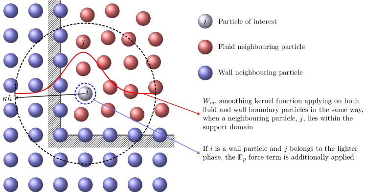
Figure 1: Schematic illustration of the wall boundary condition: The blue particles represent the dummy wall boundaries and are fixed during the entire simulation. Fluid particles (in red) interact with the dummy particles and neighbouring fluid particles that lie in the support domain. In this work we use a $5th$-order Wendland kernel (Wendland, 1995) for which $\kappa=2$.

In order to realise the fluid-wall interactions, we only need to solve the constructed Riemann problem with the following intermediate pressure between particles of fluids and wall dummy particles, the same as for fluid-fluid interactions (see section 2.2)

$$p^{*}=\frac{\rho_{f}p_{w}+\rho_{w}p_{f}}{\rho_{f}+\rho_{w}},$$ (11)

where subscripts $f$ and $w$ denote fluid and wall, respectively. This will decrease the wall-induced numerical dissipation. It is worth mentioning that the intermediate velocity value $U^{*}$ is still obtained through Eq. (8), as for fluid-fluid interactions, depending on the problem being single- or multi-phase. We next calculate the pressure of the wall dummy particles by a summation over all contributions of the neighbouring fluid particles, similar to Adami et al. (2012)

$$p_{w}=\frac{\sum_{f}p_{f}W_{wf}+(\mathbf{g}-\mathbf{a}_{w})\cdot\sum_{f}\mathbf{r}_{wf}W_{wf}}{\sum_{f}W_{wf}},$$ (12)

where $\mathbf{a}_{w}$ is the wall acceleration. Note that, for the multi-phase problems with high density ratios, the above equation is divided by $\rho_{f}$ to vanish the contribution of the heavy phase particles in $p_{w}$ at a triple point, where water, air and solid particles meet (Rezavand et al., 2020). The density of wall dummy particles is then obtained from pressure using the equation of state presented by Eq. (3). Another important aspect of this formulation is that the implementation of Eq. (12) retains the parallel nature of the algorithm related to the SPH method on GPUs (Winkler et al., 2017; Peng et al., 2019).

2.4 Penalty method

As mentioned before and seen in Eq. (2), in the present methodology we introduce a novel force balance term obtained from a penalty method, which effectively prevents particle penetration also in highly violent impacts and multi-phase flows with high density ratios. As also explained in figure 1, this force is only applied when the particles of the lighter phase (e.g. $i\in$air) interact with wall particles ($j=w$) and reads

$$\mathbf{F}_{p}=-2\sum_{w}\frac{m_{w}}{\rho_{i}\rho_{w}}\mathcal{P}\mathbf{n}_{w}\frac{1}{\left|\mathbf{r}_{iw}\right|^{2}}\frac{\partial W_{iw}}{\partial(\left|\mathbf{r}_{iw}\right|)},$$ (13)

where $\mathbf{n}_{w}$ is the estimate for the unit normal vector of the wall particles, $\frac{\partial W_{iw}}{\partial(\left|\mathbf{r}_{iw}\right|)}$ is the first derivative of the kernel function and $\mathcal{P}=\gamma_{p}\lambda|p_{i}\mathbf{e}_{iw}\cdot\mathbf{n}_{w}|$ is the penalty parameter for which $\gamma_{p}$ denotes the penalty strength and

$$\left.\begin{array}[]{ll}\displaystyle\lambda=\frac{(1-\delta)^{2}}{dx}\quad\mbox{on\ }\quad\delta<1\\[8.0pt] \displaystyle\lambda=0\quad\mbox{on\ }\quad\delta\geq 1\end{array}\right\},$$ (14)

where $dx$ is the initial particle spacing and

$$\delta=\frac{2\left|\mathbf{r}_{iw}\right|}{dx}(\mathbf{e}_{iw}\cdot\mathbf{n}_{w}).$$ (15)

In the simulations of the present study $\gamma_{p}=1$ and the unit normal vector for wall particles are calculated by (Randles & Libersky, 1996; Zhang et al., 2017)

$$\mathbf{n}_{w}=\frac{\Psi(\mathbf{r}_{i})}{\left|\Psi(\mathbf{r}_{i})\right|},\quad\mbox{with\ }\quad\Psi(\mathbf{r}_{i})=-\sum_{j\in w}\frac{m_{j}}{\rho_{j}}\nabla_{i}W_{ij},$$ (16)

where the summation is only applied on the wall particles.

2.5 Density reinitialisation

In order to further enhance the robustness and accuracy of the proposed method, we propose a simple and efficient formulation to reinitialise the density field. In this formulation, the density field of fluid particles in free-surface flows is reinitialised at every time step using the following formulation

$$\rho_{i}=\rho^{0}\frac{\sigma_{i}}{\sigma^{0}_{i}}+\max(0,~{}\rho^{*}-\rho^{0}\frac{\sigma_{i}}{\sigma^{0}_{i}})\frac{\rho^{0}}{\rho^{*}},$$ (17)

where $\sigma_{i}=\sum W_{ij}$ and $\sigma^{0}_{i}=\sum W^{0}_{ij}$ are the current and the initial number particle densities, respectively, $\rho^{*}$ denotes the density before reinitialisation and superscript $0$ represents the initial reference value. For flows without free surface, Eq. (17) is simplified as

$$\rho_{i}=\rho^{0}\frac{\sigma_{i}}{\sigma^{0}_{i}},$$ (18)

for internal flow. Note that the light phase experiences the heavy phase like moving wall boundary, while the heavy phase undergoes a free-surface-like flow with variable free-surface pressure in present multi-phase model. Therefore, Eqs. (17) and (18) are applied to light and heavy phases, respectively.

2.6 Time integration

At the beginning of every time step, the fluid density field is initialised by Eq.(17) or Eq.(18). To integrate the equations of motion in time, the kick-drift-kick (Monaghan, 2005; Adami et al., 2013) scheme is employed. The first half-step velocity is obtained as

$$\mathbf{v}_{i}^{n+\frac{1}{2}}=\mathbf{v}_{i}^{n}+\frac{\delta t}{2}\big{(}\frac{\text{d}\mathbf{v}_{i}}{\text{d}t}\big{)}^{n},$$ (19)

from which we obtain the position of particles at the next time step

$$\mathbf{r}_{i}^{n+1}=\mathbf{r}_{i}^{n}+\delta t\mathbf{v}_{i}^{n+\frac{1}{2}}.$$ (20)

Having the reinitialised density field and new positions, we update the density field either with the continuity equation in Eq.(5) and the following formulation for the heavy phases (e.g. water)

$$\rho_{i}^{n+1}=\rho_{i}^{n}+\delta t\big{(}\frac{\mathrm{d}\rho_{i}}{\mathrm{d}t}\big{)}^{n+\frac{1}{2}},$$ (21)

or solely with the summation formulation in 4 for the light phase (e.g. air). The pressure field is then updated using Eq.(3), accordingly. Now, we can obtain the time increment of the velocity field by Eq.(10) and then update the velocity of particles to the next time step as

$$\mathbf{v}_{i}^{n+1}=\mathbf{v}_{i}^{n+\frac{1}{2}}+\frac{\delta t}{2}\big{(}\frac{\text{d}\mathbf{v}_{i}}{\text{d}t}\big{)}^{n+1}.$$ (22)

For numerical stability, the time step size is limited by the CFL condition

$$\delta t\leq 0.25\big{(}\frac{h}{c+U_{max}}\big{)},$$ (23)

and the body force condition

$$\delta t\leq 0.25\sqrt{\frac{h}{\left|\mathbf{g}\right|}}.$$ (24)

It is worth noting that following our previous work (Rezavand et al., 2020), also the present method uses the same speed of sound both for light and heavy phases which considerably enhances the computational efficiency of the method.

3 GPU implementation

In recent years the utilisation of the high floating point arithmetic performance of GPUs has become increasingly more widespread for high performance scientific computing. With the heterogeneous multi-thread architectures of GPUs, this new paradigm has made it possible to execute demanding large scale simulations on general purpose computing workstations. One of the leading technologies in this scope is the Nvidia graphic cards that are able to harness the computational power of thousands of GPU cores using the compute unified device architecture (CUDA).

In this study, we have implemented the proposed methodologies in CUDA using GPU well-suited data structures. Our numerical algorithm consists of the following main compartments: a) mass and momentum conservation equations, b) density update, c) pressure calculation for the dummy boundary particles, d) neighbour search and e) time integration. All of these multiple parts are implemented as CUDA kernels to be execute fully on the device (GPU), thereby minimizing the costly communications between host (CPU) and device memories. We only need to copy the simulation data once at the beginning from host to device, and vice versa when we need to save the computational results onto host at desired time intervals. The method is fully developed on single precision floating points arithmetic, which makes it possible to be efficiently executable even on consumer graphic cards.

Table 1 shows the percentage of the computational effort for all the aforementioned compartments according to the profiling results obtained by the Nvidia nvprof profiler for a 3-D multi-phase sloshing tank problem with $243~{}432$ particles. As expected, the most resource intensive parts are the mass and momentum equations. It is noted that among the corresponding functions of the proposed wall boundary condition treatment, only the pressure calculation for wall particles and the density update formulation, respectively with 8.35% and 5.94%, take a considerable percentage of computational time. The computational effort corresponding to the penalty method and the normal vector calculation kernels are negligible. This demonstrates the efficiency of the proposed wall model on the GPU architectures, as the core kernels (penalty method and normal vectors) introduce almost no additional computational overhead and the proposed method is thus evidently computationally efficient and also well suited to GPU architectures as it also does not expose additional memory caching.

In our framework, we use a single data structure for both fluid particles and the wall dummy particles. This is possible because, as we explained in section 2.3, the dummy particles contribute in the mass and momentum conservation equations in the same way as fluid particles. For this reason there is no need to store additional data, enforced by the wall boundary model, on the limited shared memory per streaming multiprocessor (SM), which is necessary in previous wall boundary models for GPUs (see e.g. Fourtakas et al., 2019). The above-mentioned characteristics also imply that the number of operations per data element access on the device memory is quite large and it tends to be a compute-bound kernel rather a memory-bound/bandwidth-bound kernel (Lee et al., 2012; Alimirzazadeh et al., 2018). Having in mind that the computational power of the GPUs is already quite high and is still rapidly growing, i.e. the number of registers and size of caches are increasing, this will be of high importance also for further optimizations in the near future. Similar advantages have been also observed in other GPU accelerated SPH solvers employing the wall boundary model proposed by Adami et al. (2012) and running on single GPUs (see e.g. Winkler et al., 2017; Peng et al., 2019). The proposed method in the present study retains these advantages, while enhancing the accuracy, robustness and efficiency of the method of Adami et al. (2012).

CUDA kernel	Time (%)
Mass conservation (Riemann solver)	47.64
Momentum conservation (Riemann solver)	34.96
BC pressure	8.35
Density update	5.94
Neighbour search (including sorting algorithms)	2.31
Time integration	0.64
Other functions	0.16

Table 1: Percentage of the computational effort for different CUDA kernels for a 3-D multi-phase sloshing tank problem.

4 Numerical tests

In this section we first consider a two-phase hydrostatic tank with a high density ratio to assess the accuracy of the proposed method in static conditions. Other test cases including a two-phase sloshing tank and two single-phase dam break flows with complex arbitrary obstacles are also considered to validate the proposed method for modelling highly violent flows with high density ratio and to analyse the robustness of the proposed generalised method in complex 3-D problems, as well as challenging single-phase flows. We have used the quintic Wendland kernel Wendland (1995) with a smoothing length of $h=1.3dx$ and a support radius of $2.6dx$. To set the artificial speed of sound $c$, the maximum velocity is estimated as $U_{max}=2\sqrt{gH}$ according to the shallow-water theory Ritter (1982), where $H$ is the initial depth of the denser phase and $g=9.81~{}\mathrm{m.s^{-2}}$ is the gravity acceleration for all the cases.

For the execution of the simulations we have used a workstation with an Intel(R) Xeon(R) CPU E5-2603 v4 equipped by 128 GB RAM and a Nvidia GeForce RTX 2080 Ti graphics card.

4.1 Two-phase hydrostatic tank

A 2-D two-phase hydrostatic tank is first considered to evaluate the proposed method in static conditions in the presence of gravity. In this case we quantify energy conservation properties of the proposed method, assess its accuracy and also analyse the convergence characteristics of the proposed boundary condition. The lower half of the tank is filled with water and the upper half is occupied by air, both initially at rest. The schematic of this problem is illustrated in figure 2.

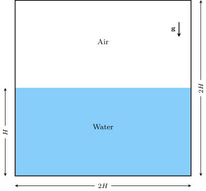
Figure 2: Two-phase hydrostatic tank: schematic illustration.

The tank has a length of $L=2H=1~{}$m and the initial water depth is $H=0.5~{}$m. Initially, particles are regularly placed on a Cartesian grid and to carry out convergence studies we use four initial particle spacings, namely $dx=0.01,~{}0.005,~{}0.0025$ and $0.00125~{}$m. The two fluids are considered to be inviscid and the density of water and air are $\rho_{w}=1000~{}\mathrm{kg\cdot m^{-3}}$ and $\rho_{a}=1~{}\mathrm{kg\cdot m^{-3}}$, respectively. The obtained pressure contours and the particle distribution are depicted in figure 3 at $t=10~{}$s. It can be observed that a quite smooth pressure field and a stable two-phase interface is obtained without notable non-physical interfacial behaviour. It is also noteworthy that both the pressure field and particle distribution in the vicinity of the wall boundaries are also quite uniform, which shows the effectiveness of the proposed wall boundary condition.

Figure 3: Two-phase hydrostatic tank: (a) particle distribution and (b) pressure field at $t=10~{}$s.

The accuracy and convergence properties of the proposed methodology are next evaluated through the comparison of the numerically computed pressure profile with the analytical hydrostatic pressure values. Figure 4 (a) compares the obtained pressure profile with the analytical solution and figure 4 (b) shows the convergence properties of the proposed method using the $L_{2}$-norm of error (Fatehi & Manzari, 2011). As it can be observed, an approximately first-order convergence is obtained.

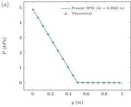
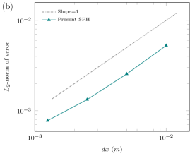
Figure 4: Two-phase hydrostatic tank: (a) comparison of the pressure profile with analytical solution and (b) $L_{2}$-norm convergence analysis at $t=10~{}$s.

As a substantial characteristic of numerical schemes, the energy conservation properties of the proposed method are also investigated here. Time histories of the global kinetic and potential energies of the system are plotted in figure 5.

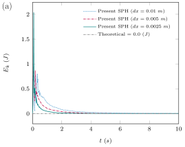
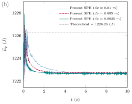
Figure 5: Two-phase hydrostatic tank: time histories of (a) global kinetic energy and (b) global potential energy of the system in comparison with analytical values and obtained with various particle resolutions.

One can clearly observe that after the initial effects of gravity, the energy variation vanishes and the system reaches an steady state. According to the results obtained with various particle resolutions, the solution evidently converges towards more accuracy with increasing resolution, however, the increased resolution of $dx=0.0025~{}$m has led to considerable noises in potential energy plot, which are due to the large number of particles contributing in the calculation of the $E_{p}$ values. Considering the obtained rest situation and having the theoretical amount of energy ($T_{tot}=1226.25~{}$J) in mind, it is concluded that the proposed method has dissipated only $0.26\%$ of the total energy until around $t=2~{}$s and the total energy stayed conserved afterwards.

4.2 Two-phase sloshing tank

The long lasting challenge of a robust wall boundary for 3-D multi-phase flows in the context of the SPH method has been subject of research since decades (Valizadeh & Monaghan, 2015). Our previously demonstrated progresses in dealing with multi-physics highly violent flows (e.g. Rezavand et al., 2020; Zhang et al., 2017, 2021a, 2021b) are further enhanced in the present study and in this section we examine the robustness and accuracy of the proposed method in one of the most challenging violent and complex multi-phase flows. If the motion frequency in a liquid sloshing tank is close to the natural frequency of the liquid due to the gravity wave, resonant condition happens, which may cause enormous impact loads on the structures. In this cases, where particles of a light phase are interacting with the wall boundaries and simultaneously with the heavy phase particles, some particles of the light phase penetrate into the wall and ultimately leave the 3-D computational domain. In this section, we also demonstrate the ability of the proposed method to effectively prevent this phenomena and compare the results with the method of Adami et al. (2012).

Due to the highly non-linear phenomena in sloshing, similar benchmark cases have been used to validate several multi-physics SPH formulations (see e.g. Khayyer et al., 2021b; Lyu & Sun, 2021; Zhang et al., 2020a; Gotoh et al., 2014). Cercos-Pita (2015) and Winkler et al. (2017) have also solved this problem on GPUs.

In this section we consider a 3-D two-phase liquid-gas sloshing case, which has been experimentally studied by Rafiee et al. (Rafiee et al., 2011). The schematic of this problem is illustrated in figure 6.

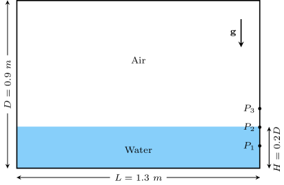
Figure 6: 3-D two-phase liquid-gas sloshing tank: schematic illustration.

A tank of height $D=0.9~{}$m and width $L=1.3~{}$m is partially filled with water to 20% of the height, i.e. $H=0.18~{}$m, while the remainder is filled by air. The flow is considered to be inviscid also in this case, where the density of water and air are set to $\rho_{w}=1000~{}\mathrm{kg\cdot m^{-3}}$ and $\rho_{a}=1~{}\mathrm{kg\cdot m^{-3}}$, respectively. The tank motion is defined by a sinusoidal excitation of $x=A_{0}sin(2.0f_{0}\pi t)$, where $A_{0}=0.1~{}$m and $f_{0}=0.496~{}\mathrm{s^{-1}}$ are the amplitude and frequency, respectively. The simulations of this section have been carried out with $dx=0.005$ m, which results in $1~{}410~{}752$ total particles. Figure 8 shows the sloshing flow evolution within the 3-D domain in different time frames. The particles are identified with their phase index and it can be seen that the multi-phase interface is well captured and the dynamic nature of the flow along with the splashing phenomena are well reproduces. Moreover, the interaction of fluid particles with the wall boundaries is efficiently simulated and no non-physical penetration is noted.

The efficiency of the proposed method in preventing the particle penetration phenomena mentioned in previous sections is detailed in figure 7. It can be clearly observed that without applying the $\mathbf{F}_{p}$ penalty force term between particles of the light phase and the wall boundary particles, several particles of the light phase have penetrated into the wall boundaries at a triple point where all three phases, namely water, air and solid walls, are present. This behaviour continues to the next time steps and the particles ultimately leave the computational domain, which violates the conservation of mass principle and causes numerical instability. The proposed method effectively prevents this non-physical behaviour and leads to accurate and stable solutions.

Figure 7: 3-D two-phase liquid-gas sloshing tank: zoom-in views of the flow simulations (a) with and (b) without the $\mathbf{F}_{p}$ penalty force term being applied between particles of the light phase and the wall boundary particles.

In order to further analyse the accuracy and performance of the proposed wall boundary condition in some cases where triple points occur, the interaction of fluid particles with wall boundaries at a triple point is shown in figure 9. It can be evidently seen that the interactions of both liquid and gas particles with the wall particles are very well reproduced, the interfaces between various phases are sharply maintained and quite smooth pressure and velocity fields are achieved. We can see that with the herein proposed wall boundary treatment an accurate and efficient interaction between fluid and wall particles is realised and non-physical penetration is prevented. Note that as the particles of the wall boundaries are constantly fixed, for easier interpretations of the figures we have not depicted them here.

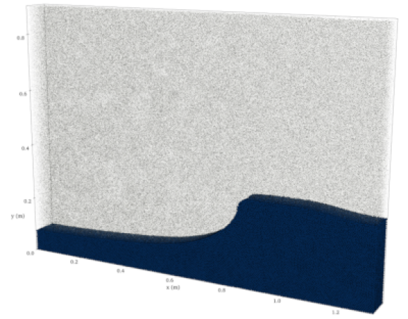
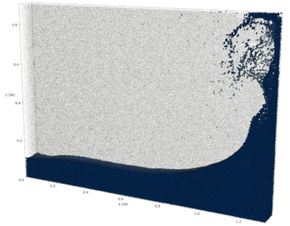
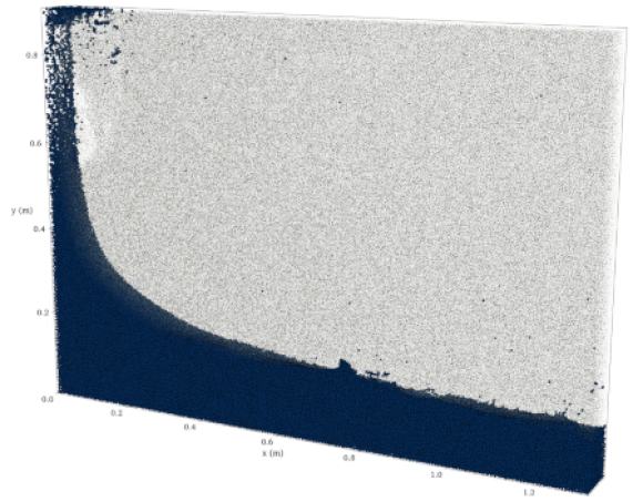
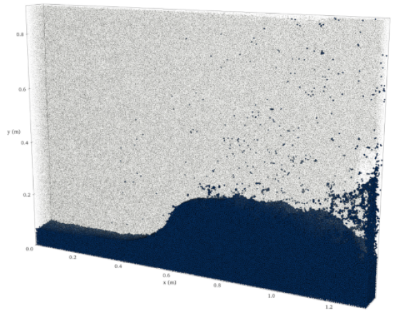
Figure 8: 3-D two-phase liquid-gas sloshing tank: snapshots of the flow evolution together with the details of multi-phase interface. The snapshots illustrate the time frames of $t=2.0,~{}3.8,~{}4.7$ and $6.25$ s and $dx=0.005~{}$m.

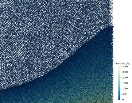
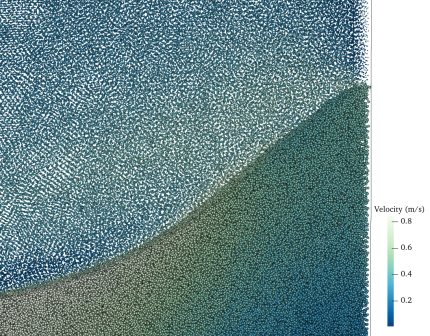
Figure 9: 3-D two-phase liquid-gas sloshing tank: zoom-in views of the (a) pressure field and (b) velocity field at a triple point where liquid, gas and solid wall particles interact at $t=1.75$ s where the first strong impact occurs.

The obtained results for the 3-D two-phase liquid-gas sloshing tank by the present method are also quantitatively validated against experimental results of Rafiee et al. (2011) in figure 10. The pressure signals at three sensors shown in figure 6 are calculated and plotted here. A good agreement is evidently achieved between the experiments and the results obtained by the presented methodology. More importantly, the peak impact pressures predicted by the present method are found to be in a clearly better agreement with the experiments in comparison to the previous two-phase and single-phase simulations of Rezavand et al. (2020) and Zhang et al. (2020a), respectively. These analysis demonstrate that the newly proposed wall boundary condition can outperform the previous methodologies in the simulation of highly violent impacts and prediction of the impact pressure, while achieves also more accurate simulations.

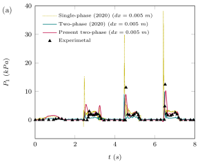
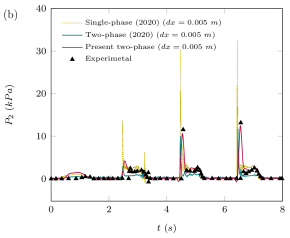
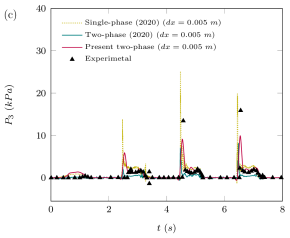
Figure 10: 3-D two-phase liquid-gas sloshing tank: time histories of the impact pressure at (a) $P_{1}$, (b) $P_{2}$ and (c) $P_{3}$ sensors in comparison with the experimental results of Rafiee et al. (2011), previous two-phase SPH simulations of Rezavand et al. (2020) and single-phase SPH simulations of Zhang et al. (2020a)

4.3 Dam break with an obstacle

In this section we consider a 3-D dam break case with an obstacle placed on the downstream horizontal bed, which is known as the SPHERIC benchmark #2 and its detailed description can be found in https://spheric-sph.org/tests/test-2. This test case has been studied by Kleefsman et al. (2005) first experimentally and then by an Eulerian volume of fluid (VOF) method. Later, this test case was simulated with the standard WCSPH and truly incompressible SPH (ISPH) methods by Lee et al. (2010) and was recently also studied using a weakly compressible moving particle semi-implicit (WCMPS) by Jandaghian et al. (2021). In our simulations, particles are initially placed regularly on a Cartesian grid and in order to further analyse the convergence properties of the proposed method, we carry out the simulations with three different particle resolutions, viz. $dx=0.032,~{}0.016$ and $0.008~{}$m, which correspond to $69~{}773$, $349~{}340$ and $2~{}061~{}483$ number of particles, respectively.

The evolution of the breaking dam flow is illustrated in several snapshots in figures 11 and 12, where the contours of pressure and velocity fields are shown, respectively. All physical features of the flow are very well captured and the distribution of both pressure and velocity fields are quite smooth at the vicinity of the solid walls, as well as the free-surface. The interaction of the water flow with the obstacle at $t=0.6~{}$s is also very well reproduced and the splash-up after the surge wave impacts the obstacle is well exhibited. The above observations demonstrate the effectiveness and accuracy of the proposed wall boundary treatment.

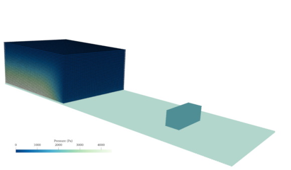
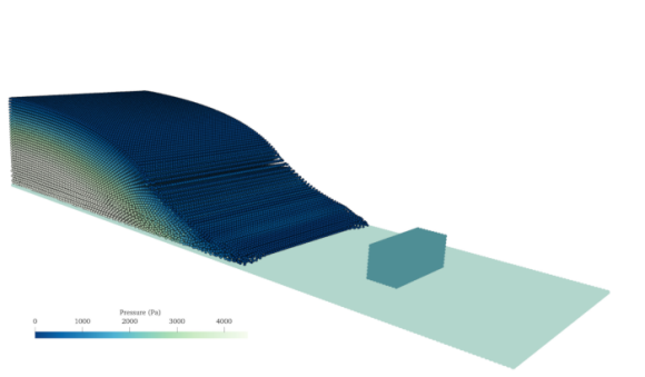
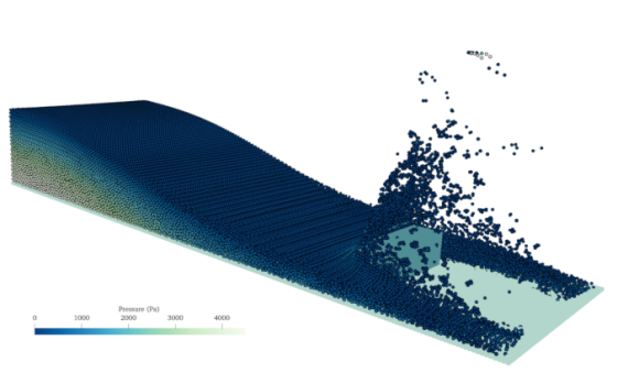
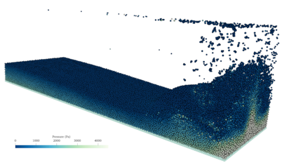
Figure 11: 3-D dam break with obstacle: snapshots of the flow evolution together with pressure distribution within the domain. The snapshots illustrate the time frames of $t=0,~{}0.3,~{}0.6$ and $1.2$ s and $dx=0.016~{}$m.

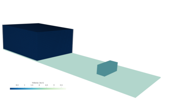
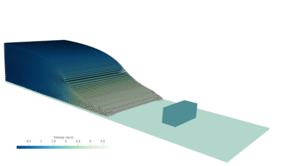
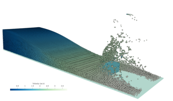
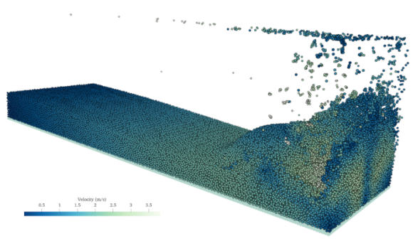
Figure 12: 3-D dam break with obstacle: snapshots of the flow evolution together with velocity distribution within the domain. The snapshots illustrate the time frames of $t=0,~{}0.3,~{}0.6$ and $1.2$ s and $dx=0.016~{}$m.

In order to further validate the accuracy of the proposed method, we quantitatively compare the values of impact pressure ($P_{i},~{}i=1,\,\ldots,\,4$) and wave height ($H_{i},~{}i\in\{2,3,4\}$) obtained from seven sensors as describes in the test case documentation with the same names. The measured pressure signals are obtained by the method explained by Zhang et al. (2017). The pressure signals cause by the violent impact of the generated water wave are compared against experiments of Kleefsman et al. (2005) in figure 13. A good agreement is noted between the present SPH simulations and the experimental results. The peak impact pressure signals are well captured and also the long-term behaviours of the residual pressures are well reproduced. The pressure peak at sensor $P_{4}$ is slightly underestimated by the proposed method, however, the calculated pressure signals converge to the experimental results as the particle resolution increases. The sensor $P_{4}$ is located at the top of the obstacle with the presence of free-surface and effects of air, which might have caused the underestimation. A similar behaviour is however reported also by Mokos et al. (2017) for both higher sensors ($P_{3}$ and $P_{4}$) although they have carried out multi-phase simulation with the consideration of the air phase. It can be observed that our proposed wall treatment has evidently improved the pressure predictions in comparison to their multi-phase simulation for both challenging sensors, $P_{3}$ and $P_{4}$.

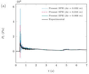
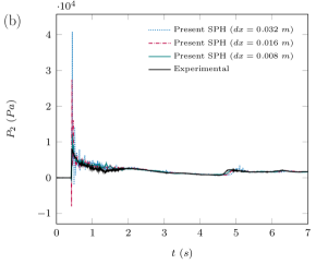
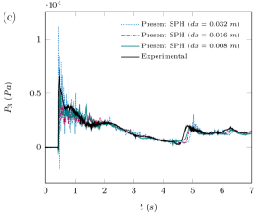
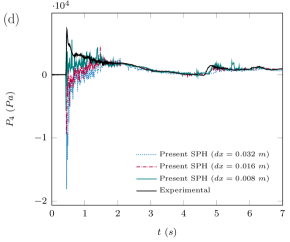
Figure 13: 3-D dam break with obstacle: time histories of the impact pressure at (a) $P_{1}$, (b) $P_{2}$, (c) $P_{3}$ and (d) $P_{4}$ sensors with different particle resolutions and in comparison with the experimental results of Kleefsman et al. (2005).

Figure 14 portrays the time history of the water levels recorded at three different probes as identified by the experiment documentation. A good agreement with the experiments is noted also here and the long-term behaviour of wave height is well reproduced. The run-up and the water level peaks are slightly overestimated, which are attributed to the inviscid nature of the method that, as discussed in 4.1, introduces a marginal energy dissipation. It is also worth noting that in these plots the proposed method demonstrates a reasonable rate of convergence, as seen also in previous test cases.

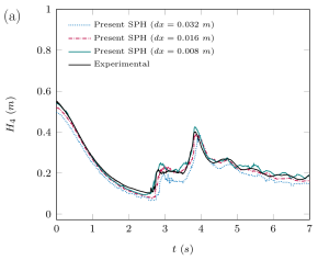
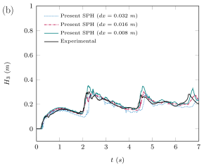
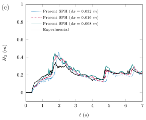
Figure 14: 3-D dam break with obstacle: time histories of the wave height at (a) $H_{4}$, (b) $H_{3}$ and (c) $H_{2}$ with different particle resolutions and in comparison with the experimental results of Kleefsman et al. (2005).

4.4 Dam break with a wedge

Sharp boundaries and accurate reproduction of the resulting fluid-wall interactions have also always been a challenge for the SPH method. In order to further asses the proposed method in 3-D arbitrary geometries with sharp boundaries, here we consider a dam break flow with a wedge located at the middle of the downstream bed. The configuration of the problem is described in figure 15. A similar 2-D test case has already been used by Valizadeh & Monaghan (2015), however, we consider a wedge of $\pi/3$ rad angle, which results in sharper geometries and more abrupt changes in the flow pattern. The height of the wedge is $h_{w}=5.5~{}$m and here we set an initial inter-particle distance of $dx=h_{w}/40$ corresponding to $5~{}734~{}250$ number of particles.

Figure 15: 3-D dam break with a wedge: schematic illustration.

The evolution of the breaking dam flow and its interactions with the wedge are illustrated in several snapshots in figures 16 and 17, with the contours of pressure and velocity fields being shown, respectively. All physical features of the flow are very well captured and the distribution of both pressure and velocity fields are quite smooth. The interaction of water with the wedge at $t=4~{}$s and also the water jet formed after the wedge are effectively simulated. The above observations demonstrate the effectiveness and accuracy of the proposed wall boundary treatment. As it can be also observed, the large number of particles has resulted in simulations with more details of the flow structure.

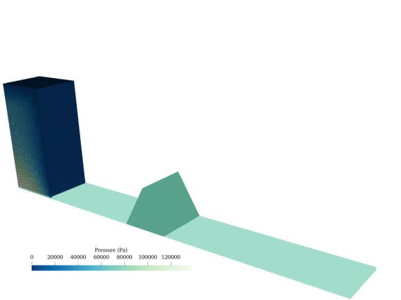
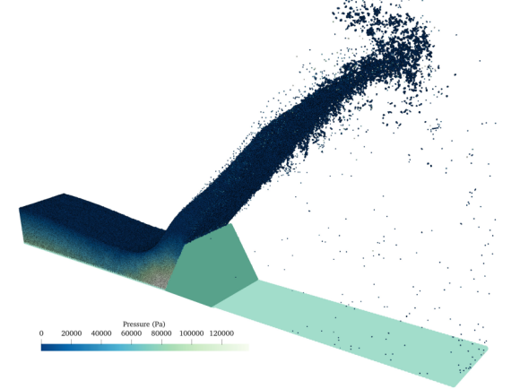
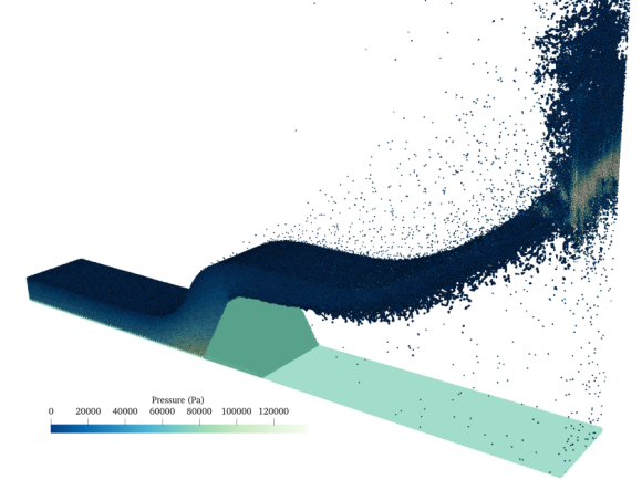
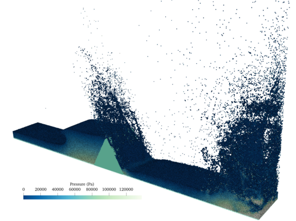
Figure 16: 3-D dam break with a wedge: snapshots of the flow evolution together with pressure distribution within the domain. The snapshots illustrate the time frames of $t=0,~{}4,~{}6$ and $8$ s and $dx=0.138~{}$m.

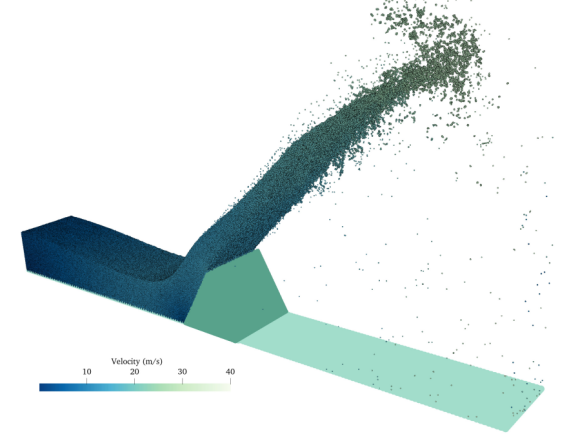
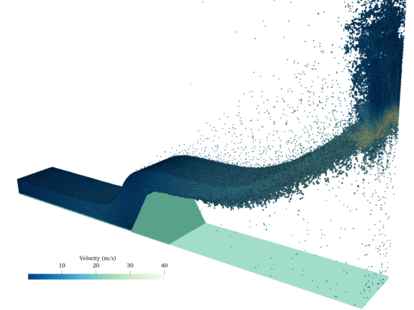
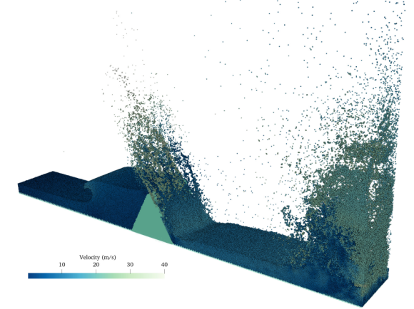
Figure 17: 3-D dam break with a wedge: snapshots of the flow evolution together with velocity distribution within the domain. The snapshots illustrate the time frames of $t=0,~{}4,~{}6$ and $8$ s and $dx=0.138~{}$m.

The interaction of the high-speed water flow with the wedge is illustrated in more details in figure 18. It can be seen that the free-surface, particle splashing and the interaction with wedge are accurately simulated. The pressure and velocity fields are also quite smoothly captured. It is also worth mentioning that the effect of the sharp upper tip of the wedge on the flow pattern is very well noted, where it deviates the water particles from their relatively straight trajectory led by the water jet.

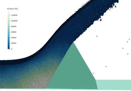
Figure 18: 3-D dam break with a wedge: zoom-in views of the (a) pressure field and (b) velocity field at $t=4$ s where the water flow interacts with the wedge and a high-speed water jet is developed.

5 Concluding remarks

In this study, we have presented a robust and efficient wall boundary condition for the SPH method which is accurately generalised for arbitrary 3-D complex geometries, multi-phase flows, and highly dynamic problems. As it has been concluded by Valizadeh & Monaghan (2015), the wall boundary condition treatment presented by Adami et al. (2012) in combination with a density diffusion formulation achieves the most satisfactory results among the widely used methodologies in the field of SPH. The presented method in this paper, generalises the method of Adami et al. (2012) for complex 3-D problems, as well as multi-phase flows, while improves its accuracy, robustness and efficiency.

The proposed methodology is also implemented using CUDA to be executed on GPUs. Various specifications of the method are discussed and profiling results of the GPU-accelerated framework are summarized. The analysis highlights that the GPU kernel functions corresponding to the proposed method impose negligible computational overhead and memory caching, which identifies that the proposed methodology is ideally suited to the heterogeneous architecture of GPUs.

The proposed method is validated against existing experimental data, previous numerical studies and analytical solutions for both single- and multi-phase problems. It is shown that accurate solutions are obtained and potential non-physical particle penetration into the walls are prevented. Furthermore, it is evidently exhibited that in predicting violent impact events, the proposed method outperforms the previous methodologies of Rezavand et al. (2020) and Zhang et al. (2020a), which have employed the wall boundary treatment proposed by Adami et al. (2012). Concerning arbitrary configurations with sharp geometries, the proposed method performs also very well and obtains accurate simulation, reproducing substantial features of the flows and fluid-wall interactions.

As the presented wall boundary condition exhibits unprecedented accuracy and is also efficiently executable on GPUs with no additionally imposed computational overhead, the method is a reliable solution for the long-lasting challenge of the wall boundary condition in the SPH method for a broad range of natural and industrial applications.

References

- Adami et al. (2012) Adami, S., Hu, X.Y. & Adams, N.A. 2012 A generalized wall boundary condition for smoothed particle hydrodynamics. J. Comput. Phys. 231 (21), 7057 – 7075.
- Adami et al. (2013) Adami, S, Hu, XY & Adams, Nikolaus A 2013 A transport-velocity formulation for smoothed particle hydrodynamics. J. Comput. Phys. 241, 292–307.
- Alimirzazadeh et al. (2018) Alimirzazadeh, Siamak, Jahanbakhsh, Ebrahim, Maertens, Audrey, Leguizamón, Sebastián & Avellan, François 2018 Gpu-accelerated 3-d finite volume particle method. Computers & Fluids 171, 79–93.
- Antuono et al. (2012) Antuono, Matteo, Colagrossi, Andrea & Marrone, Salvatore 2012 Numerical diffusive terms in weakly-compressible sph schemes. Computer Physics Communications 183 (12), 2570–2580.
- Cercos-Pita (2015) Cercos-Pita, Jose L 2015 Aquagpusph, a new free 3d sph solver accelerated with opencl. Computer Physics Communications 192, 295–312.
- Crespo et al. (2015) Crespo, Alejandro JC, Domínguez, José M, Rogers, Benedict D, Gómez-Gesteira, Moncho, Longshaw, S, Canelas, RJFB, Vacondio, Renato, Barreiro, Anxo & García-Feal, O 2015 Dualsphysics: Open-source parallel cfd solver based on smoothed particle hydrodynamics (sph). Computer Physics Communications 187, 204–216.
- Fatehi & Manzari (2011) Fatehi, R & Manzari, MT 2011 Error estimation in smoothed particle hydrodynamics and a new scheme for second derivatives. Computers & Mathematics with Applications 61 (2), 482–498.
- Fourtakas et al. (2019) Fourtakas, Georgios, Dominguez, Jose M, Vacondio, Renato & Rogers, Benedict D 2019 Local uniform stencil (lust) boundary condition for arbitrary 3-d boundaries in parallel smoothed particle hydrodynamics (sph) models. Computers & Fluids 190, 346–361.
- Fraga Filho et al. (2019) Fraga Filho, Carlos Alberto Dutra, Peng, Chong, Ibne Islam, Md Rushdie, McCabe, Christopher, Baig, Samiullah & Durga Prasad, Gonella Venkata 2019 Implementation of three-dimensional physical reflective boundary conditions in mesh-free particle methods for continuum fluid dynamics: Validation tests and case studies. Physics of Fluids 31 (10), 103606.
- Gotoh et al. (2014) Gotoh, Hitoshi, Khayyer, Abbas, Ikari, Hiroyuki, Arikawa, Taro & Shimosako, Kenichiro 2014 On enhancement of incompressible sph method for simulation of violent sloshing flows. Applied Ocean Research 46, 104–115.
- Hérault et al. (2010) Hérault, Alexis, Bilotta, Giuseppe & Dalrymple, Robert A. 2010 SPH on GPU with CUDA. Journal of Hydraulic Research 48 (Extra Issue), 74–79.
- Hopp-Hirschler et al. (2019) Hopp-Hirschler, Manuel, Shadloo, Mostafa Safdari & Nieken, Ulrich 2019 Viscous fingering phenomena in the early stage of polymer membrane formation. Journal of Fluid Mechanics 864, 97–140.
- Jandaghian et al. (2021) Jandaghian, Mojtaba, Krimi, Abdelkader, Zarrati, Amir Reza & Shakibaeinia, Ahmad 2021 Enhanced weakly-compressible mps method for violent free-surface flows: Role of particle regularization techniques. Journal of Computational Physics 434, 110202.
- Khayyer et al. (2021a) Khayyer, Abbas, Gotoh, Hitoshi, Shimizu, Yuma & Nishijima, Yusuke 2021a A 3d lagrangian meshfree projection-based solver for hydroelastic fluid–structure interactions. Journal of Fluids and Structures 105, 103342.
- Khayyer et al. (2021b) Khayyer, Abbas, Shimizu, Yuma, Gotoh, Hitoshi & Hattori, Shunsuke 2021b Multi-resolution isph-sph for accurate and efficient simulation of hydroelastic fluid-structure interactions in ocean engineering. Ocean Engineering 226, 108652.
- Kleefsman et al. (2005) Kleefsman, KMT, Fekken, G, Veldman, AEP, Iwanowski, B & Buchner, B 2005 A volume-of-fluid based simulation method for wave impact problems. Journal of computational physics 206 (1), 363–393.
- Kulasegaram et al. (2004) Kulasegaram, Sivakumar, Bonet, Javier, Lewis, RW & Profit, M 2004 A variational formulation based contact algorithm for rigid boundaries in two-dimensional sph applications. Computational Mechanics 33 (4), 316–325.
- Lee et al. (2012) Lee, Daren, Dinov, Ivo, Dong, Bin, Gutman, Boris, Yanovsky, Igor & Toga, Arthur W 2012 Cuda optimization strategies for compute-and memory-bound neuroimaging algorithms. Computer methods and programs in biomedicine 106 (3), 175–187.
- Lee et al. (2010) Lee, Eun-Sug, Violeau, Damien, Issa, Réza & Ploix, Stéphane 2010 Application of weakly compressible and truly incompressible sph to 3-d water collapse in waterworks. Journal of Hydraulic Research 48 (S1), 50–60.
- Libersky et al. (1993) Libersky, Larry D, Petschek, Albert G, Carney, Theodore C, Hipp, Jim R & Allahdadi, Firooz A 1993 High strain lagrangian hydrodynamics: a three-dimensional sph code for dynamic material response. Journal of computational physics 109 (1), 67–75.
- Luo et al. (2021) Luo, Min, Khayyer, Abbas & Lin, Pengzhi 2021 Particle methods in ocean and coastal engineering. Applied Ocean Research 114, 102734.
- Lyu & Sun (2021) Lyu, Hong-Guan & Sun, Peng-Nan 2021 Further enhancement of the particle shifting technique: towards better volume conservation and particle distribution in sph simulations of violent free-surface flows. Applied Mathematical Modelling .
- Marongiu et al. (2010) Marongiu, Jean-Christophe, Leboeuf, Francis, Caro, JoËlle & Parkinson, Etienne 2010 Free surface flows simulations in pelton turbines using an hybrid sph-ale method. Journal of Hydraulic Research 48 (S1), 40–49.
- Mayrhofer et al. (2015) Mayrhofer, Arno, Ferrand, Martin, Kassiotis, Christophe, Violeau, Damien & Morel, François-Xavier 2015 Unified semi-analytical wall boundary conditions in sph: analytical extension to 3-d. Numerical Algorithms 68 (1), 15–34.
- Mokos et al. (2017) Mokos, Athanasios, Rogers, Benedict D & Stansby, Peter K 2017 A multi-phase particle shifting algorithm for SPH simulations of violent hydrodynamics with a large number of particles. J. Hydraul. Res. 55 (2), 143–162.
- Monaco et al. (2011) Monaco, Antonio Di, Manenti, Sauro, Gallati, Mario, Sibilla, Stefano, Agate, Giordano & Guandalini, Roberto 2011 Sph modeling of solid boundaries through a semi-analytic approach. Engineering Applications of Computational Fluid Mechanics 5 (1), 1–15.
- Monaghan (1994) Monaghan, Joe J 1994 Simulating free surface flows with sph. J. Comput. Phys. 110 (2), 399–406.
- Monaghan (2005) Monaghan, J J 2005 Smoothed particle hydrodynamics. Rep. Prog. Phys. 68 (8), 1703.
- Monaghan (2012) Monaghan, J. J. 2012 Smoothed Particle Hydrodynamics and Its Diverse Applications. Annu. Rev. Fluid Mech. 44 (1), 323–346.
- Monaghan & Kajtar (2009) Monaghan, Joe J & Kajtar, Jules B 2009 Sph particle boundary forces for arbitrary boundaries. Computer physics communications 180 (10), 1811–1820.
- Moussa et al. (2006) Moussa, Bachir Ben & others 2006 On the convergence of SPH method for scalar conservation laws with boundary conditions. Methods Appl. Anal. 13 (1), 29–62.
- Peng et al. (2019) Peng, Chong, Wang, Shun, Wu, Wei, Yu, Hai-sui, Wang, Chun & Chen, Jian-yu 2019 Loquat: an open-source gpu-accelerated sph solver for geotechnical modeling. Acta Geotechnica 14 (5), 1269–1287.
- Rafiee et al. (2011) Rafiee, Ashkan, Pistani, Fabrizio & Thiagarajan, Krish 2011 Study of liquid sloshing: numerical and experimental approach. Comput. Mech. 47 (1), 65–75.
- Rahmat et al. (2020) Rahmat, Amin, Weston, Daniel, Madden, Daniel, Usher, Shane, Barigou, Mostafa & Alexiadis, Alessio 2020 Modeling the agglomeration of settling particles in a dewatering process. Physics of Fluids 32 (12), 123314, arXiv: https://doi.org/10.1063/5.0029213.
- Randles & Libersky (1996) Randles, PW & Libersky, Larry D 1996 Smoothed particle hydrodynamics: some recent improvements and applications. Computer methods in applied mechanics and engineering 139 (1-4), 375–408.
- Rezavand et al. (2018) Rezavand, Massoud, Taeibi-Rahni, Mohammad & Rauch, Wolfgang 2018 An ISPH scheme for numerical simulation of multiphase flows with complex interfaces and high density ratios. Comput. Math. Appl. 75 (8), 2658–2677.
- Rezavand et al. (2019) Rezavand, Massoud, Winkler, Daniel, Sappl, Johannes, Seiler, Laurent, Meister, Michael & Rauch, Wolfgang 2019 A fully lagrangian computational model for the integration of mixing and biochemical reactions in anaerobic digestion. Computers & Fluids 181, 224–235.
- Rezavand et al. (2020) Rezavand, Massoud, Zhang, Chi & Hu, Xiangyu 2020 A weakly compressible sph method for violent multi-phase flows with high density ratio. Journal of Computational Physics 402, 109092.
- Ritter (1982) Ritter, August 1982 Die fortpflanzung der wasserwellen. Zeitschrift des Vereines Deutscher Ingenieure 36 (33), 947–954.
- Shimizu et al. (2020) Shimizu, Yuma, Khayyer, Abbas, Gotoh, Hitoshi & Nagashima, Ken 2020 An enhanced multiphase isph-based method for accurate modeling of oil spill. Coastal Engineering Journal pp. 1–22.
- Toro (1989) Toro, EF 1989 A fast Riemann solver with constant covolume applied to the random choice method. Int. J. Numer. Methods Fluids 9 (9), 1145–1164.
- Vacondio et al. (2020) Vacondio, Renato, Altomare, Corrado, De Leffe, Matthieu, Hu, Xiangyu, Le Touzé, David, Lind, Steven, Marongiu, Jean-Christophe, Marrone, Salvatore, Rogers, Benedict D & Souto-Iglesias, Antonio 2020 Grand challenges for smoothed particle hydrodynamics numerical schemes. Computational Particle Mechanics pp. 1–14.
- Valizadeh & Monaghan (2015) Valizadeh, Alireza & Monaghan, Joseph J 2015 A study of solid wall models for weakly compressible sph. Journal of Computational Physics 300, 5–19.
- Vázquez-Quesada et al. (2019) Vázquez-Quesada, Adolfo, Español, Pep, Tanner, Roger I & Ellero, Marco 2019 Shear thickening of a non-colloidal suspension with a viscoelastic matrix. Journal of Fluid Mechanics 880, 1070–1094.
- Vila (1999) Vila, JP 1999 On particle weighted methods and smooth particle hydrodynamics. Math. Models Methods Appl. Sci. 9 (02), 161–209.
- Wendland (1995) Wendland, Holger 1995 Piecewise polynomial, positive definite and compactly supported radial functions of minimal degree. Adv. Comput. Math. 4 (1), 389–396.
- Winkler et al. (2017) Winkler, Daniel, Meister, Michael, Rezavand, Massoud & Rauch, Wolfgang 2017 gpuSPHASE–A shared memory caching implementation for 2D SPH using CUDA. Comput. Phys. Commun. 213, 165 – 180.
- Zhang et al. (2017) Zhang, Chi, Hu, XY & Adams, Nikolaus A 2017 A weakly compressible SPH method based on a low-dissipation Riemann solver. J. Comput. Phys. 335, 605–620.
- Zhang et al. (2020a) Zhang, Chi, Rezavand, Massoud & Hu, Xiangyu 2020a Dual-criteria time stepping for weakly compressible smoothed particle hydrodynamics. Journal of Computational Physics 404, 109135.
- Zhang et al. (2021a) Zhang, Chi, Rezavand, Massoud & Hu, Xiangyu 2021a A multi-resolution sph method for fluid-structure interactions. Journal of Computational Physics 429, 110028.
- Zhang et al. (2021b) Zhang, Chi, Rezavand, Massoud, Zhu, Yujie, Yu, Yongchuan, Wu, Dong, Zhang, Wenbin, Wang, Jianhang & Hu, Xiangyu 2021b Sphinxsys: an open-source multi-physics and multi-resolution library based on smoothed particle hydrodynamics. Computer Physics Communications p. 108066.
- Zhang et al. (2020b) Zhang, Chi, Rezavand, Massoud, Zhu, Yujie, Yu, Yongchuan, Wu, Dong, Zhang, Wenbin, Zhang, Shuoguo, Wang, Jianhang & Hu, Xiangyu 2020b Sphinxsys: An open-source meshless, multi-resolution and multi-physics library. Software Impacts 6, 100033.
- Zhang et al. (2021c) Zhang, Chi, Wang, Jianhang, Rezavand, Massoud, Wu, Dong & Hu, Xiangyu 2021c An integrative smoothed particle hydrodynamics method for modeling cardiac function. Computer Methods in Applied Mechanics and Engineering 381, 113847.