VC dimension of partially quantized neural networks in the overparametrized regime

Abstract

Vapnik-Chervonenkis (VC) theory has so far been unable to explain the small generalization error of overparametrized neural networks. Indeed, existing applications of VC theory to large networks obtain upper bounds on VC dimension that are proportional to the number of weights, and for a large class of networks, these upper bound are known to be tight. In this work, we focus on a class of partially quantized networks that we refer to as hyperplane arrangement neural networks (HANNs). Using a sample compression analysis, we show that HANNs can have VC dimension significantly smaller than the number of weights, while being highly expressive. In particular, empirical risk minimization over HANNs in the overparametrized regime achieves the minimax rate for classification with Lipschitz posterior class probability. We further demonstrate the expressivity of HANNs empirically. On a panel of 121 UCI datasets, overparametrized HANNs match the performance of state-of-the-art full-precision models.

1 Introduction

Neural networks have become an indispensable tool for machine learning practitioners, owing to their impressive performance especially in vision and natural language processing (Goodfellow et al., 2016). In practice, neural networks are often applied in the overparametrized regime and are capable of fitting even random labels (Zhang et al., 2021). Evidently, these overparametrized models perform well on real world data despite their ability to grossly overfit, a phenomenon that has been dubbed “the generalization puzzle” (Nagarajan & Kolter, 2019).

Toward solving this puzzle, several research directions have flourished and offer potential explanations, including implicit regularization (Chizat & Bach, 2020), interpolation (Chatterji & Long, 2021), and benign overfitting (Bartlett et al., 2020). So far, VC theory has not been able to explain the puzzle, because existing bounds on the VC dimensions of neural networks are on the order of the number of weights (Maass, 1994; Bartlett et al., 2019). It remains unknown whether there exist neural network architectures capable of modeling rich set of classfiers with low VC dimension.

The focus of this work is on a class of neural networks with threshold activation that we refer to as hyperplane arrangement neural networks (HANNs). Using the theory of sample compression schemes (Littlestone & Warmuth, 1986), we show that HANNs can have VC dimension that is significantly smaller than the number of parameters. Furthermore, we apply this result to show that HANNs have high expressivity by proving that HANN classifiers achieve minimax-optimality when the data has Lipschitz posterior class probability in an overparametrized setting.

We benchmark the empirical performance of HANNs on a panel of 121 UCI datasets, following several recent neural network and neural tangent kernel works (Klambauer et al., 2017; Wu et al., 2018; Arora et al., 2019; Shankar et al., 2020). In particular, Klambauer et al. (2017) showed that, using a properly chosen activation, overparametrized neural networks perform competitively compared to classical shallow methods on this panel of datasets. Our experiments show that HANNs, a partially-quantized model, match the classification accuracy of the self-normalizing neural network (Klambauer et al., 2017) and the dendritic neural network (Wu et al., 2018), both of which are full-precision models.

1.1 Related work

VC dimensions of neural networks. The VC-dimension Vapnik & Chervonenkis (1971) is a combinatorial measure of the complexity of a concept class, i.e., a set of classifiers. The Fundamental Theorem of Statistical Learning (Shalev-Shwartz & Ben-David, 2014, Theorem 6.8) states that a concept class has finite VC-dimension if and only if it is probably approximately correct (PAC) learnable, where the VC-dimension is tightly related to the number of samples required for PAC learning.

For threshold networks, Cover (1965); Baum & Haussler (1989) showed a VC-dimension upper bounded of $O(w\log w)$, where $w$ is the number of parameters. Maass (1994) obtained a matching lower bound attained by a network architecture with two hidden layers. More recently, Bartlett et al. (2019) obtained the upper and lower bounds $O(w\ell\log w)$ and $\Omega(w\ell\log(w/\ell))$ respectively for the case when the activation is piecewise linear, where $\ell$ is the number of layers. These lower bounds are achieved by somewhat unconventional network architectures. The architectures we consider exclude these and thus we are able to achieve a smaller upper bound on the VC dimensions.

The generalization puzzle. In practice, neural networks that achieve state-of-the-art performance use significantly more parameters than samples, a phenomenon that cannot be explained by classical VC theory if the VC dimension $\geq$ number of weights. This has been dubbed the generalization puzzle (Zhang et al., 2021). To explain the puzzle, researchers have pursued new directions including margin-based bounds (Neyshabur et al., 2017; Bartlett et al., 2017), PAC-Bayes bounds (Dziugaite & Roy, 2017), and implicit bias of optimization methods (Gunasekar et al., 2018; Chizat & Bach, 2020). We refer the reader to the recent article by Bartlett et al. (2021) for a comprehensive coverage of this growing literature.

The generalization puzzle is not specific to deep learning. For instance, AdaBoost has been observed to continue to decrease the test error while the VC dimension grows linearly with the number of boosting rounds (Schapire, 2013). Other learning algorithms that exhibits similarly surprising behavior include random forests (Wyner et al., 2017) and kernel methods (Belkin et al., 2018).

Minimax-optimality. Whereas VC theory is distribution-independent, minimax theory is concerned with the question of optimal estimation/classification under distributional assumptions. A minimax optimality result shows that the expected excess classification error goes to zero at the fastest rate possible, as the sample size tend to infinity. For neural networks, this often involves a hyperparameter selection scheme in terms of the sample size.

Faragó & Lugosi (1993) show minimax-optimality of (underparametrized) neural networks for learning to classify under certain assumptions on the Fourier transform of the data distribution. Schmidt-Hieber (2020) shows minimax-optimality of $s$-sparse neural networks for regression over Hölder classes, where at most $s=O(n\log n)$ network weights are nonzero, and $n=$ the number of training samples. Kim et al. (2021) extends the results of Schmidt-Hieber (2020) to the classification setting, remarking that effective optimization under sparsity constraint is lacking. Kohler & Langer (2020) and Langer (2021) proved minimax-optimality without the sparsity assumption, however in an underparametrized setting. To the best of our knowledge, our result is the first to establish minimax optimality of overparametrized neural networks without a sparsity assumption.

(Partially) quantized neural networks. Quantizing some of the weights and/or activations of neural networks has the potential to reduce the high computational burden of neural networks at test time (Qin et al., 2020). Many works have focused on the efficient training of quantized neural networks to close the performance gap with full-precision architectures (Hubara et al., 2017; Rastegari et al., 2016; Lin et al., 2017). Several works have observed that quantization of the activations, rather than of the weights, leads to a larger accuracy gap (Cai et al., 2017; Mishra et al., 2018; Kim et al., 2019).

Towards explaining this phenomenon, researchers have focused on understanding the so-called coarse gradient, a term coined by Yin et al. (2019), often used in training QNNs as a surrogate for the usual gradient. One commonly used heuristic is the straight-through-estimator (STE) first introduced in an online course by Hinton et al. (2012). Theory supporting the STE heuristic has recently been studied in Li et al. (2017) and Yin et al. (2019).

QNNs have also been analyzed from other theoretical angles, including mean-field theory (Blumenfeld et al., 2019), memory capacity (Vershynin, 2020), Boolean function representation capacity (Baldi & Vershynin, 2019) and adversarial robustness (Lin et al., 2018). Of particular relevance to our work, Maass (1994) constructed an example of a QNN architecture with VC dimension on the order of the number of weights in the network. In contrast, our work shows that there exist QNN architectures with much smaller VC dimensions.

Sample compression schemes. Many concept classes with geometrically structured decision regions, such as axis-parallel rectangles, can be trained on a properly chosen size $\sigma$ subset of an arbitrarily large training dataset without affecting the result. Such a concept class is said to admit a sample compression schemes of size $\sigma$, a notion introduced by Littlestone & Warmuth (1986) who showed that the VC dimension of the class is upper bounded by $O(\sigma)$. Furthermore, the authors posed the Sample Compression Conjecture. See Moran & Yehudayoff (2016) for the best known partial result and an extensive review of research in this area. Besides the conjecture, sample compression schemes have also been applied to other long-standing problems in learning theory (Hanneke et al., 2019; Bousquet et al., 2020; Ashtiani et al., 2020). To the best of our knowledge, our work is the first to apply sample compression schemes to neural networks.

2 Notations

The set of real numbers is denoted $\mathbb{R}$. The unit interval is denoted $[0,1]$. For an integer $k\geq 1$, let $[k]=\{1,\dots,k\}$. We use $\mathcal{X}$ to denote the feature space, which in this work will either be $\mathbb{R}^{d}$ or $[0,1]^{d}$ where $d\geq 1$ is the ambient dimension/number of features.

Denote by $\mathbb{I}\{\mathtt{input}\}$ the indicator function which returns $1$ if $\mathtt{input}$ is true and $0$ otherwise. The sign function is given by $\sigma_{\mathtt{sgn}}(t)=\mathbb{I}\{t\geq 0\}-\mathbb{I}\{t<0\}$. For vector inputs, $\sigma_{\mathtt{sgn}}$ applies entry-wise.

The set of labels for binary classification is denoted $\mathbb{B}:=\{\pm 1\}$. Joint distributions on $\mathcal{X}\times\mathbb{B}$ are denoted by $P$, where $X,Y\sim P$ denotes a random instance-label pair distributed according to $P$. Let $f:\mathcal{X}\to\mathbb{B}$ be a binary classifier. The risk with respect to $P$ is denoted by $R_{P}(f):=P(f(X)\neq Y)$. For an integer $n\geq 1$, the empirical risk is the random variable $\hat{R}_{P,n}(f):=\frac{1}{n}\sum_{i=1}^{n}\mathbb{I}\{f(X_{i})\neq Y_{i}\}$, where $(X_{1},Y_{1}),\dots,(X_{n},Y_{n})\sim P$ are i.i.d. The Bayes risk $\inf_{f:\mathcal{X}\to\mathbb{B}}R_{P}(f)$ with respect to $P$ is denoted by $R_{P}^{*}$.

Let $f,g:\{1,2,\dots\}\to\mathbb{R}_{\geq 0}$ be nonnegative functions on the natural numbers. We write $f\asymp g$ if there exists $\alpha,\beta>0$ such that for all $n=1,2,\dots$ we have $\alpha g(n)\leq f(n)\leq\beta g(n)$.

3 Hyperplane arrangement neural networks

A hyperplane $H$ in $\mathbb{R}^{d}$ is specified by its normal vector ${w}\in\mathbb{R}^{d}$ and bias $b\in\mathbb{R}$. The mapping $x\mapsto\sigma_{\mathtt{sgn}}({w}^{\top}x+b)$ indicates the side of $H$ that $x$ lies on, and hence induces a partition of $\mathbb{R}^{d}$ into two halfspaces. A set of $k\geq 1$ hyperplanes is referred to as a $k$-hyperplane arrangement, and specified by a matrix of normal vectors and a vector of offsets:

$$\mathbf{W}=[{w}_{1}\cdots{w}_{k}]\in\mathbb{R}^{d\times k}\quad\mbox{and}\quad{b}=[b_{1},\dots,b_{k}]^{\top}.$$

Let $q_{\mathbf{W},{b}}(x):=\sigma_{\mathtt{sgn}}(\mathbf{W}^{\top}x+{b})$ for all $x\in\mathbb{R}^{d}.$ The vector $q_{\mathbf{W},{b}}(x)\in\mathbb{B}^{k}$ is called a sign vector and the set of all realizable sign vectors is denoted $\mathfrak{S}_{\mathbf{W},{b}}:=\{q_{\mathbf{W},{b}}(x):x\in\mathbb{R}^{d}\}.$ Each sign vector ${s}\in\mathfrak{S}_{\mathbf{W},{b}}$ uniquely defines a set $\{x\in\mathbb{R}^{d}:q_{\mathbf{W},{b}}(x)={s}\}$ known as a cell of the hyperplane arrangement. The set of all cells forms a partition of $\mathbb{R}^{d}$. For an example, see Figure 1-left.

A classical result in the theory of hyperplane arrangement due to Buck (1943) gives the following tight upper bound on the number of distinct sign patterns/cells:

$$|\mathfrak{S}_{\mathbf{W},{b}}|\leq\binom{k}{\leq d}:=\begin{cases}2^{k}&:k<d,\\ \binom{k}{0}+\binom{k}{1}+\cdots+\binom{k}{d}&:k\geq d.\end{cases}$$ (1)

See Fukuda (2015) Theorem 10.1 for a simple proof. A hyperplane arrangement classifier assigns a binary label $y\in\mathbb{B}$ to a point $x\in\mathbb{R}^{d}$ solely based on the sign vector $q_{\mathbf{W},{b}}(x)$.

Figure 1: Left: An arrangement of $3$ hyperplanes $\{H_{1},H_{2},H_{3}\}$ in $\mathbb{R}^{2}$. There are $7$ sign patterns. Middle: An example of a lookup table (see Remark 3.2). Right: the resulting classifier.

Definition 3.1.

Let $\mathbb{B}^{\mathcal{X}}$ be the set of all functions from $\mathcal{X}$ to $\mathbb{B}$. A concept class $\mathcal{C}$ over $\mathcal{X}$ is a subset of $\mathbb{B}^{\mathcal{X}}$. Fix $r,k$ positive integers, $r\leq\min\{d,k\}$. Let $\mathtt{Bool}_{k}$ be the set of all Boolean functions $\mathbb{B}^{k}\to\mathbb{B}$. The hyperplane arrangement classifier class is the concept class, denoted $\mathtt{HAC}(d,r,k)$, over $\mathbb{R}^{d}$ defined by

$$\mathtt{HAC}(d,r,k)=\{h\circ q_{\mathbf{W},{b}}:\,\, h\in\mathtt{Bool}_{k},\,q_{\mathbf{W},{b}}(x):=\sigma_{\mathtt{sgn}}(\mathbf{W}^{\top}x+{b}),$$

$$\mathbf{W}\in\mathbb{R}^{d\times k},\,\mathrm{rank}(\mathbf{W})\leq r,\,{b}\in\mathbb{R}^{k}\}.$$

See Figure 2 for a graphical representation of $\mathtt{HAC}(d,r,k)$. When the set of Boolean functions is realized by a neural network, we refer to the resulting classifier as a hyperplane arrangement neural network (HANN).

Remark 3.2.

Consider a fixed hyperplane arrangement $\mathbf{W}$, ${b}$ and Boolean function $h\in\mathtt{Bool}_{k}$. When performing prediction with the classifer $h\circ q_{\mathbf{W},{b}}$, the feature vector $x$ is mapped to a sign vector to which $h$ is applied. Thus, we do not need to know how $h$ behaves outside of $\mathfrak{S}_{\mathbf{W},{b}}$. The restriction of $h$ to $\mathfrak{S}_{\mathbf{W},{b}}$ is a partially defined Boolean function or a lookup table.

Figure 2: The $\mathtt{HAC}(d,r,k)$ concept class as a neural network where $d=4$, $r=2$ and $k=3$. The Boolean function $h$ is realized as a neural network $h_{\theta}$.

Remark 3.3.

The hidden layer of width $r$ in Figure 2 allows the user to impose the restriction that the hyperplane arrangement classifier depends only on $r$ relevant features, which can be either learned or defined by data preprocessing. When $r=d$, no restriction is imposed. In this case, the input layer is directly connected to the Boolean layer. This is consistent with Definition 3.1 where the rank constraint $\mathrm{rank}(\mathbf{W})\leq r$ becomes trivial.

Our next goal is to upper bound the VC dimension of $\mathtt{HAC}(d,r,k)$.

Definition 3.4 (VC-dimension).

Let $\mathcal{C}\subseteq\mathbb{B}^{\mathcal{X}}$ be a concept class over $\mathcal{X}$. A set $S:=\{x_{1},\dots,x_{n}\}\subseteq\mathcal{X}$ is shattered by $\mathcal{C}$ if for all sequences $(y_{1},\dots,y_{n})\in\mathbb{B}^{n}$, there exists $f\in\mathcal{C}$ such that $f(x_{i})=y_{i}$ for all $i\in[n]$. The VC-dimension of $\mathcal{C}$ is defined as

$$\mathtt{VC}(\mathcal{C})=\sup\{|S|:S\subseteq\mathcal{X},\,\mbox{$S$ is shattered by $\mathcal{C}$}\}.$$

The VC-dimension has many far-reaching consequences in learning theory and, in particular, classification. One of these consequences is a sufficient (in fact also necessary) condition for uniform convergence in the sense of the following well-known theorem. See Shalev-Shwartz & Ben-David (2014) Theorem 6.8.

Theorem 3.5.

Let $\mathcal{C}$ be a concept class over $\mathcal{X}$. There exists a constant $C>0$ such that for all joint distributions $P$ on $\mathcal{X}\times\mathbb{B}$ and all $f\in\mathcal{C}$, we have $|\hat{R}_{P,n}(f)-R_{P}(f)|\leq C\sqrt{(\mathtt{VC}(\mathcal{C})+\log(1/\delta))/{n}}$ with probability at least $1-\delta$ with respect to the draw of $(X_{1},Y_{1}),\dots,(X_{n},Y_{n})$.

Note that the above VC bound is useless in the overparametrized setting if $\mathtt{VC}(\mathcal{C})=\Omega(\mbox{\# of weights})$. We now present our main result: an upper bound on the VC dimension of $\mathtt{HAC}(d,r,k)$.

Theorem 3.6.

Let $d,r,k\geq 1$ be integers and $\mathtt{HAC}(d,r,k)$ be defined as in Definition 3.1. Then

$$\mathtt{VC}(\mathtt{HAC}(d,r,k))\leq 8\cdot\left(k(d+1)+k(d+1)(1+\lceil\log_{2}k\rceil)+\binom{k}{\leq r}\right).$$

In the next section, we will prove this result using a sample compression scheme. Before proceeding, we comment on the significance of the result.

Remark 3.7.

Since $\binom{k}{\leq r}=O(k^{r})$, we have $\mathtt{VC}(\mathtt{HAC}(d,r,k))=O(k^{r}+dk\log k)$ which only involves the input dimension $d$ and the width of the first two hidden layers $r$ and $k$. For constant $d$ and $r\geq 2$, this reduces to $\mathtt{VC}(\mathtt{HAC}(d,r,k))=O(k^{r})$. In particular, the number of weights used by an architecture to implement the Boolean function $h$ does not affect the VC dimension at all.

For instance, Mukherjee & Basu (2017) Lemma 2.1 states that a 1-hidden layer neural network with ReLU activation can model any $k$-input Boolean function if the hidden layer has width $\geq 2^{k}$. Note that this network uses $\geq k2^{k}$ weights, and $k2^{k}\gg k^{r}$ for fixed $r$ and $k$ large.

Baldi & Vershynin (2019) study implementation of Boolean functions using threshold networks. A consequence of their Theorem 9.3 is that a 2-hidden layer network with widths $\geq c2^{k/2}/\sqrt{k}$ can implement all $k$ input Boolean functions, where $c$ is a constant not depending on $k$. This requires $\geq c^{2}2^{k}/k$ weights which again is exponentially larger than $k^{r}$. Furthermore, this lower bound on the weights is also necessary as $k\to\infty$.

4 A sample compression scheme

In this section, we will construct a sample compression scheme for $\mathtt{HAC}(d,r,k)$. As alluded to in the Related Work section, the size of a sample compression scheme upper bounds the VC-dimension of a concept class, which will be applied to prove Theorem 3.6. We first recall the definition of sample compression schemes with side information introduced in Littlestone & Warmuth (1986).

Definition 4.1.

Let $\mathcal{C}$ be a concept class. A length $n$ sequence $\{(x_{i},y_{i})\in\mathcal{X}\times\mathbb{B}\}_{i\in[n]}$ is $\mathcal{C}$-labelled if there exists $f\in\mathcal{C}$ such that $f(x_{i})=y_{i}$ for all $i\in[n]$. Denote by $L_{\mathcal{C}}(n)$ the set of $\mathcal{C}$-labelled sequences of length at most $n$. Denote by $L_{\mathcal{C}}(\infty)$ the set of all $\mathcal{C}$-labelled sequences of finite length. The concept class $\mathcal{C}$ over $\mathcal{X}$ has an $m$-sample compression scheme with $s$-bits of side information if there exists a pair of maps $(\rho,\kappa)$ where

$$\kappa:L_{\mathcal{C}}(\infty)\to L_{\mathcal{C}}(m)\times\mathbb{B}^{s},\quad\rho:L_{\mathcal{C}}(m)\times\mathbb{B}^{s}\to\mathbb{B}^{\mathcal{X}}$$

such that for all $\mathcal{C}$-labelled sequences $S:=\{(x_{i},y_{i})\}_{i\in[n]}$, we have $\rho(\kappa(S))(x_{i})=y_{i}$ for all $i\in[n]$. The size of the sample compression scheme is $\mathtt{size}(\rho,\kappa):=m+s$.

Intuitively, $\kappa$ and $\rho$ can be thought of as the compression and the reconstruction maps, respectively. The compression map $\kappa$ keeps $m$ elements from the training set and $s$ bits of additional information, which $\rho$ uses to reconstruct a classifier that correctly labels the uncompressed training set.

The main result of this section is:

Theorem 4.2.

$\mathtt{HAC}(d,r,k)$ has a sample compression scheme $(\rho,\kappa)$ of size

$$\mathtt{size}(\rho,\kappa)=k(d+1)+k(d+1)(1+\lceil\log_{2}k\rceil)+\binom{k}{\leq r}.$$

The rest of this section will work toward the proof of Theorem 4.2. The following result states that a $\mathcal{C}$-labelled sequence can be labelled by a hyperplane arrangement classifier of a special form.

Proposition 4.3.

Let $\{(x_{i},y_{i})\}_{i\in[n]}$ be $\mathtt{HAC}(d,r,k)$-labelled. Then there exist $\mathbf{V}=[{v}_{1}\cdots{v}_{k}]\in\mathbb{R}^{d\times k},{c}\in\mathbb{R}^{k}$ and $h\in\mathtt{Bool}_{k}$ such that for all $i\in[n]$, we have 1) $y_{i}=h(\sigma_{\mathtt{sgn}}(\mathbf{V}^{\top}x_{i}+{c}))$, 2) $\mathrm{rank}(\mathbf{V})\leq r$ and 3) $|{v}_{j}^{\top}x_{i}+c_{j}|\geq 1$ for all $i\in[n],j\in[k]$.

The proof, given in Appendix A.1, is similar to showing the existence of a max-margin separating hyperplane for a linearly separable dataset.

Definition 4.4.

Let $I$ be a finite set and let ${a}_{i}\in\mathbb{R}^{n}$ for each $i\in I$. Let $A=\{{a}_{i}\}_{i\in I}$. A conical combination of $A$ is a linear combination $\sum_{i\in I}\lambda_{i}{a}_{i}$ where the weights $\lambda_{i}\in\mathbb{R}_{\geq 0}$ are nonnegative. The conical hull of $A$, denoted $\mathtt{coni}(A)$, is the set of all conical combinations of $A$, i.e., $\mathtt{coni}(\{{a}_{i}\}_{i\in I}):=\left\{\sum_{i\in I}\lambda_{i}{a}_{i}:\lambda_{i}\in\mathbb{R}_{\geq 0},\,\forall i\in I\right\}.$

The result below follows easily from the Carathédory’s theorem for the conical hull (Lovász & Plummer, 2009). For the sake of completeness, we included the proof in Appendix A.2.

Proposition 4.5.

Let ${a}_{1},\dots,{a}_{m}\in\mathbb{R}^{n}$ and $b_{1},\dots,b_{m}\in\mathbb{R}$. For each subset $I\subseteq[m]$, define

$$\mathcal{P}_{I}:=\{x\in\mathbb{R}^{n}:{a}_{i}^{\top}x\leq b_{i}\,\forall i\in I\}.$$

Then 1) $\min_{x\in\mathcal{P}_{I}}\frac{1}{2}\|x\|^{2}$ has a unique minimizer, denoted by $x^{*}_{I}$ below, and 2) there exists a subset $J\subseteq[m]$ such that $|J|=n$ and for all $I\subseteq[m]$ with $J\subseteq I$, we have $x^{*}_{[m]}=x^{*}_{I}$.

Proof of Theorem 4.2.

Let $(x_{i},y_{i})$ be $\mathtt{HAC}(d,r,k)$-realizable, and $\mathbf{V},{c}$ and $h$ be as in Proposition 4.3. For each $i\in[n]$, define the Boolean vectors ${s}_{i}:=\sigma_{\mathtt{sgn}}(\mathbf{V}^{\top}x_{i}+{c})\in\{\pm 1\}^{k}$ and $s_{ij}=\sigma_{\mathtt{sgn}}({v}_{j}^{\top}x_{i}+c_{j})$ denote the $j$-th entry of ${s}_{i}$. Note that $s_{ij}({v}_{j}^{\top}x_{i}+c_{j})=|{v}_{j}^{\top}x_{i}+c_{j}|\geq 1$.

We first outline the steps of the proof:

1. Using a subset of the samples $\{(x_{i_{\ell}},y_{i_{\ell}}):\ell\in[d(k+1)]\}$ with additional $k(d+1)(1+\lceil\log_{2}k\rceil)$ bits of side information $\{(s_{i_{\ell}j_{\ell}},j_{\ell}):\ell\in[d(k+1)]\}$, we can reconstruct $\overline{\mathbf{W}},\overline{{b}}$ such that $\sigma_{\mathtt{sgn}}(\overline{\mathbf{W}}^{\top}x_{i}+\overline{{b}})={s}_{i}$ for all $i\in[n]$.

2. Using an additional subset of samples $\{(x_{\iota_{\ell}},y_{\iota_{\ell}}):\ell=1,\dots,\binom{k}{\leq r}\}$ in conjunction with the $\overline{\mathbf{W}},\overline{{b}}$ reconstructed in the previous step, we can find $g\in\mathtt{Bool}_{k}$ such that $g(s_{i})=h(s_{i})$ for all $i$.

Now, consider the set

$$\mathcal{P}:=\left\{(\mathbf{W},{b})\in\mathbb{R}^{d\times k}\times\mathbb{R}^{k}:s_{ij}({w}_{j}^{\top}x_{i}+b_{j})\geq 1,\,\forall i\in[n],\,j\in[k]\right\}.$$

Note that $\mathcal{P}$ is a convex polyhedron in $(d+1)k$-dimensional space. Let $(\overline{\mathbf{W}},\overline{{b}})$ be the minimum norm element of $\mathcal{P}$. Note that $\sigma_{\mathtt{sgn}}(\overline{\mathbf{W}}^{\top}x_{i}+\overline{{b}})=\sigma_{\mathtt{sgn}}(\mathbf{V}^{\top}x_{i}+{c})={s}_{i}$ by construction.

By Proposition 4.5, there exists a set of tuples

$$\left\{(i_{\ell},j_{\ell})\right\}_{\ell=1,\dots,(d+1)k},\mbox{ where }(i_{\ell},j_{\ell})\in[n]\times[k]$$

such that $\overline{\mathbf{W}},\overline{{b}}$ is also the minimum norm element of

$$\mathcal{P}^{\prime}:=\left\{(\mathbf{W},{b})\in\mathbb{R}^{d\times k}\times\mathbb{R}^{k}:s_{i_{\ell}j_{\ell}}({w}_{j_{\ell}}^{\top}x_{i_{\ell}}+{b}_{j_{\ell}})\geq 1,\,\ell=1,\dots,d(k+1)\right\}.$$

To encode the defining equations of $\mathcal{P}^{\prime}$, we need to store

samples $$\{(x_{i_{\ell}},y_{i_{\ell}})\}_{\ell=1}^{d(k+1)} \{(s_{i_{\ell}j_{\ell}},j_{\ell})\}_{\ell=1}^{d(k+1)}$$ and side information . (2)

Note that each $s_{i_{\ell}j_{\ell}}$ requires $1$ bit while each $j_{\ell}\in[k]$ requires $\lceil\log_{2}k\rceil$ bits. In total, encoding $\mathcal{P}^{\prime}$ requires storing $d(k+1)$ samples and $d(k+1)(1+\lceil\log_{2}k\rceil)$ of bits.

To reconstruct $g\in\mathtt{Bool}_{k}$ that agrees with $h$ on all the samples, it suffices to know $h$ when restricted to $\{{s}_{i}\}_{i=1}^{n}$. Since $\{{s}_{i}\}_{i=1}^{n}$ is a subset of $\mathfrak{S}_{\overline{\mathbf{W}},\overline{{b}}}$, we have by eq. 1 that $|\{{s}_{i}\}_{i}^{n}|\leq\binom{k}{\leq r}$. Thus, $\{{s}_{i}\}_{i=1}^{n}$ has at most $\binom{k}{\leq r}$ unique elements. Let $\left\{{s}_{{\iota}_{\ell}}:\ell=1,\dots,\binom{k}{\leq r}\right\}$ be a set containing all such unique elements. Thus, we store

$$\mbox{samples $\{(x_{\iota_{\ell}},y_{\iota_{\ell}}):\ell=1,\dots,\binom{k}{\leq r}\}$}.$$ (3)

Using $\overline{\mathbf{W}},\overline{{b}}$ as defined above, we have ${s}_{\iota_{\ell}}=\sigma_{\mathtt{sgn}}(\overline{\mathbf{W}}^{\top}x_{\iota_{\ell}}+\overline{{b}})$. Now, simply choose $g$ such that $g({s}_{\iota_{\ell}})=y_{\iota_{\ell}}$ for all $\ell=1,\dots,\binom{k}{\leq r}$.

To summarize, we formally define the compression and reconstruction functions $(\kappa,\rho)$. Let $\kappa$ take the full sample $\{(x_{i},y_{i})\}_{i=1}^{n}$ and output the subsample (and side information) in eq. 2 and eq. 3. The reconstruction function $\rho$ first constructs $\overline{\mathbf{W}},\overline{{b}}$ using eq. 2. Next, $\rho$ constructs $g$ using $\overline{\mathbf{W}},\overline{{b}}$ and the samples of eq. 3. ∎

Now, the following result together with the sample compression scheme for $\mathtt{HAC}(d,r,k)$ we constructed imply Theorem 3.6 from the previous section.

Theorem 4.6 (Littlestone & Warmuth (1986)).

If $\mathcal{C}$ has sample compression scheme $(\rho,\kappa)$, then $\mathtt{VC}(\mathcal{C})\leq 8\cdot\mathtt{size}(\rho,\kappa)$.

Remark 4.7.

Note that the reconstruction function $\rho$ is not permutation-invariant. Furthermore, the overall sample compression scheme $\rho,\kappa$ is not stable in the sense of Hanneke & Kontorovich (2021). In general, sample compression schemes with permutation-invariant $\rho$ (Floyd & Warmuth, 1995) and stable sample compression schemes (Hanneke & Kontorovich, 2021) enjoy tighter generalization bounds compared to ordinary sample compression schemes. We leave as an open question whether $\mathtt{HAC}(d,r,k)$ has such specialized compression schemes.

5 Minimax-optimality for learning Lipschitz class

In this section, we show that empirical risk minimization (ERM) over $\mathtt{HAC}(d,r,k)$, for properly chosen $r$ and $k$, is minimax optimal for classification where the posterior class probability function is $L$-Lipschitz, for fixed $L>0$. Furthermore, the choices for $r$ and $k$ is such that the associated HANN, the neural network realization of $\mathtt{HAC}(d,r,k)$, is overparametrized for the Boolean function implementations discussed in Remark 3.7.

Below, let $X\in[0,1]^{d}$ and $Y\in\mathbb{B}$ be the random variables corresponding to a sample and label jointly distributed according to $P$. Write $\eta_{P}(x):=P(Y=1|X=x)$ for the posterior class probability function.

Let $\Sigma(L,[0,1]^{d})$ denote the class of $L$-Lipschitz functions $f:[0,1]^{d}\to\mathbb{R}$, i.e.,

$$|f(x)-f(x^{\prime})|\leq L\|x-x^{\prime}\|_{2},\quad\forall x,x^{\prime}\in[0,1]^{d}.$$

The following minimax lower bound result concerns classification when $\eta_{P}$ is $L$-Lipschitz:

Theorem 5.1 (Audibert & Tsybakov (2007)).

There exists a constant $C>0$ such that

$$\inf_{\tilde{f}_{n}}\sup_{P\,:\,\eta_{P}\in\Sigma(L,[0,1]^{d})}\mathbb{E}[R(\tilde{f}_{n})]-R^{*}_{P}\geq Cn^{-\frac{1}{d+2}}.$$

The infimum above is taken over all possible learning algorithms $\tilde{f}_{n}$, i.e., mappings from $(\mathcal{X}\times\mathbb{B})^{n}$ to Borel measurable functions $\mathcal{X}\to\mathbb{B}$. When $\hat{f}_{n}$ is an empirical risk minimizer (ERM) over $\mathtt{HAC}(d,r,k)$ where $d=r$ for $k=n^{\frac{1}{d+2}}$ , this minimax rate is achieved.

Theorem 5.2.

Let $d\geq 1$ be fixed. Let $\hat{f}_{n}$ be an ERM over $\mathtt{HAC}(d,d,k)$ where $k=k(n)\asymp n^{\frac{1}{d+1}}$. Then there exists a constant $C^{\prime}$ such that

$$\sup_{P\,:\,\eta_{P}\in\Sigma(L,[0,1]^{d})}\mathbb{E}[R(\hat{f}_{n})]-R^{*}_{P}\leq C^{\prime}n^{-\frac{1}{d+2}}.$$

Proof sketch (see Appendix A.3 for full proof). We first show that the histogram classifier over the standard partition of $[0,1]^{d}$ into smaller cubes is an element of $\mathcal{C}:=\mathtt{HAC}(d,d,k)$, thus reducing the problem to proving minimax-optimality of the histogram classifier. Previous work Györfi et al. (2006) Theorem 4.3 established this for the histogram regressor. The analogous result for the histogram classifier, to the best of our knowledge, has not appeared in the literature and thus is included for completeness.

The neural network implementation of $\mathtt{HAC}(d,d,k)$ where $k\asymp n^{1/(d+2)}$ in Theorem 5.2 can be overparametrized. Using either the 1- or the 2-hidden layer neural network implementations of Boolean functions as in Remark 3.7, the resulting HANN is overparametrized and has number of weights either $\geq k2^{k}$ or $\geq c^{2}2^{k}/k$ respectively. Both lower bounds on the number of weights are exponentially larger than $n$ meanwhile $\mathtt{VC}(\mathtt{HAC}(d,d,k))=o(n)$.

6 Empirical results

In this section, we discuss experimental results of using HANNs for classifying synthetic and real datasets. Our implementation uses TensorFlow (Abadi et al., 2016) with the Larq (Geiger & Team, 2020) library for training neural networks with threshold activations. Note that Theorem 5.2 holds for ERM over HANNs, which is intractable in practice.

Synthetic datasets. We apply a HANN (model specification shown in Figure 3-top left) to the moons synthetic dataset with two classes with the hinge loss.

The heuristic for training networks with threshold activation can significantly affect the performance (Kim et al., 2019). We consider two of the most popular heuristics: the straight-through-estimator (SteSign) and the SwishSign, introduced by Hubara et al. (2017) and Darabi et al. (2019), respectively. SwishSign reliably leads to higher validation accuracy (Figure 3-bottom left), consistent with the finding of Darabi et al. (2019). Subsequently, we use SwishSign and plot a learned decision boundary in Figure 3-right.

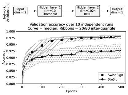
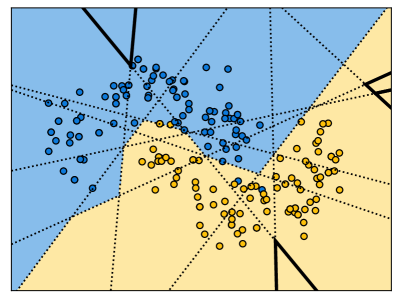
Figure 3: Top left. Architecture of HANN used for the moons dataset. Bottom left. Validation accuracies from 10 independent runs with random initialization and data generation. Right. Data points (circles) drawn from make_moons in sklearn colored by ground truth labels. The hyperplane arrangement is denoted by dotted lines. Coloring of the cells corresponds to the decision region of the trained classifier. A cell $\Delta$ is highlighted by bold boundaries if 1) no training data lies in $\Delta$ and 2) $\Delta$ does not touch the decision boundary.

By Mukherjee & Basu (2017) Lemma 2.1, any Boolean function $\mathbb{B}^{k}\to\mathbb{B}$ can be implemented by a 1-hidden layer ReLU network with $2^{k}$ hidden nodes. Here, the width of the hidden layer is $2^{10}=1024$. Thus, the architecture in Figure 3 can assign labels to the bold boundary cells arbitrarily without changing the training loss. Nevertheless, the optimization appears to be biased toward a topologically simpler classifier. This behavior is consistently reproducible. See Figure 7.

Real-world datasets. Klambauer et al. (2017) introduced self-normalizing neural networks (SNN) which were shown to outperform other neural networks on a panel of 121 UCI datasets. Subsequently, Wu et al. (2018) proposed the dendritic neural network architecture, which further improved classification performance on this panel of datasets. Following their works, we evaluate the performance of HANNs on the 121 UCI datasets.

A crucial hyperparameter for HANN is $k$, the number of hyperplanes used. We ran the experiments with $k\in\{15,100\}$ to test the hyperparameter’s impact on accuracy. The Boolean function $h$ is implemented as a 1-hidden layer residual network (He et al., 2016) of width $1000$.

We use the same train, validation, and test sets from the public code repository of Klambauer et al. (2017). The reported accuracies on the held-out test set are based on the best performing model according to the validation set. The models will be referred to as HANN15 and HANN100, respectively. The results are shown in Figure 4. The accuracies of SNN and DENN are obtained from Table A1 in the supplemental materials of Wu et al. (2018). Full details for the training and accuracy tables can be found in the appendix.

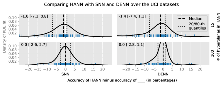
Figure 4: Each blue tick above the x-axis represents a single dataset, where the x-coordinate of the tick is the difference of the accuracy of HANN and either SNN (left) or DENN (right) on the dataset. The solid black curves are kernel density estimates for the blue ticks. The number of hyperplanes used by HANN is either 15 (top) or 100 (bottom). The quantities shown in the top-left corner of each subplot are the median, 20-th and 80-th quantiles of the differences, respectively, rounded to 1 decimal place.

The HANN15 model (top row of Figure 4) already achieves median accuracy within 1.5% of both SNN and DENN. With the larger HANN100 model (bottom row), the gap is reduced to zero. The largest training set in this panel of datasets has size $77904$. The HANN15 and HANN100 models use $\approx 10^{4}$ and $10^{5}$ weights, respectively. By comparison, the average number of weights used by SNN is $\geq 5*10^{5}$, while the number of weights used by DENN is at least $\geq 2.5*10^{5}$. Thus, all three models considered here, namely HANN, SNN and DENN, are overparametrized for this panel of datasets.

7 Discussion

We have introduced an architecture for which the VC theorem can be used to prove minimax-optimality of ERM over HANNs in an overparametrized setting with Lipschitz posterior. To our knowledge, this is the first time VC theory has been used to analyze the performance of a neural network in the overparametrized regime. Furthermore, the same architecture leads to state-of-the-art performance over a benchmark collection of unstructured datasets.

Reproducibility Statement

All code for downloading and parsing the data, training the models, and generating plots in this manuscript are available at https://github.com/YutongWangUMich/HANN. Complete proofs for all novel results are included in the main article or in an appendix.

Appendix A Proofs

A.1 Proof of Proposition 4.3

By definition, there exists $h\in\mathtt{Bool}_{k}$, $\mathbf{W}\in\mathbb{R}^{d\times k}$ of rank at most $r$, and ${b}\in\mathbb{R}^{k}$ such that $y_{i}=h(\sigma_{\mathtt{sgn}}(\mathbf{W}^{\top}x_{i}+{b}))$.

Now, let $j\in[k]$ be fixed. Since $|{w}_{j}^{\top}x_{i}+b_{j}|\geq 0$ for all $i\in[n]$, there exists a small perturbation $\tilde{c}_{j}$ of $b_{j}$ such that $|{w}_{j}^{\top}x_{i}+\tilde{c}_{j}|>0$ for all $i\in[n]$. Now, let $\lambda_{j}:=\min_{i\in[n]}|{w}_{j}^{\top}x_{i}+\tilde{c}_{j}|$ which is positive. Define ${v}_{j}:={w}_{j}/\lambda_{j}$ and $c_{j}=\tilde{c}_{j}/\lambda_{j}$, we have $|{v}_{j}^{\top}x_{i}+c_{j}|\geq 1$ for all $i\in[n]$, as desired. Note that $\mathrm{rank}(\mathbf{V})=\mathrm{rank}(\mathbf{W})$. $\Box$

A.2 Proof of Proposition 4.5

Let $g_{i}(x)={a}_{i}^{\top}x-b_{i}$ for each $i\in[m]$ and $f(x)=\frac{1}{2}\|x\|^{2}_{2}$. Then $\nabla f(x)=x$ and $\nabla g_{i}(x)={a}_{i}$. By definition, $x_{I}^{*}$ is a minimizer of

$$\min_{x\in\mathbb{R}^{n}}f(x)\mbox{ s.t. }g_{i}(x)\leq 0,\,\forall i\in I,$$

which is a convex optimization with strongly convex objective. Thus, the minimizer $x_{I}^{*}$ is unique and furthermore is the unique element $x$ of $\mathbb{R}^{n}$ satisfying the KKT conditions:

$$x\in\mathcal{P}_{I}\mbox{ and }\exists\mbox{ a set of nonnegative weights $\{\lambda_{i}\}_{i\in I}$ such that }-x=\sum_{i\in I}\lambda_{i}{a}_{i}.$$

Thus, $x_{I}^{*}$ can be equivalently characterized as the unique element of $x\in\mathbb{R}^{n}$ satisfying

$$x\in\mathcal{P}_{I}\mbox{ and }-x\in\mathtt{coni}(\{{a}_{i}\}_{i\in I}).$$ (4)

In particular, $x_{[m]}^{*}\in\mathcal{P}_{[m]}$ and $-x_{[m]}^{*}\in\mathtt{coni}(\{{a}_{i}\}_{i\in[m]})$. By the Carathédory’s theorem for the conical hull (Lovász & Plummer, 2009), there exists $\underline{I}\subseteq[m]$ such that $|\underline{I}|=n$ and $-x_{[m]}^{*}\in\mathtt{coni}(\{{a}_{i}\}_{i\in\underline{I}})$. Thus, for any $J\subseteq[m]$ such that $\underline{I}\subseteq J$, we have $-x_{[m]}^{*}\in\mathtt{coni}(\{{a}_{i}\}_{i\in J})$. Furthermore, $J\subseteq[m]$ implies $\mathcal{P}_{J}\supseteq\mathcal{P}_{[m]}$. In particular, $x_{[m]}^{*}\in\mathcal{P}_{J}$. Putting it all together, we have $x_{[m]}^{*}\in\mathcal{P}_{J}$ and $-x_{[m]}^{*}\in\mathtt{coni}(\{{a}_{i}\}_{i\in J})$. By the uniqueness, we have $x_{J}^{*}=x_{[m]}^{*}$. $\Box$

A.3 Proof of Theorem 5.2

In this proof, the constant $C$ does not depending on $n$, and may change from line to line.

We fix a joint distribution $P$ such that $\eta_{P}\in\Sigma(L,[0,1]^{d})$ throughout the proof. Thus, the notation for risks will omit the $P$ in their subscript, e.g., we write $\hat{R}_{n}(f)$ instead of $\hat{R}_{P,n}(f)$ and $R^{*}$ instead of $R^{*}_{P}$. Below, let $\beta>\alpha>0$ be constants such that $\alpha dn^{1/(d+2)}\leq k\leq\beta dn^{1/(d+2)}$. Let $\tilde{k}:=\lceil k/d\rceil$.

Let $\mathcal{R}_{1},\mathcal{R}_{2},\dots,\mathcal{R}_{\tilde{k}^{d}}$ denote the hypercubes of side length $\ell=1/\tilde{k}$ forming a partition of $[0,1]^{d}$. For each $i\in[\tilde{k}^{d}]$, let $\mathcal{R}_{i}^{-}:=\{x\in\mathcal{R}_{i}:\eta_{P}(x)<1/2\}$ and $\mathcal{R}_{i}^{+}:=\{x\in\mathcal{R}_{i}:\eta_{P}(x)\geq 1/2\}$.

Let $\tilde{f}:[0,1]^{d}\to\mathbb{B}$ be the classifier such that

$$\tilde{f}(x)=\begin{cases}+1&:x\in\mathcal{R}_{i},\,\int_{\mathcal{R}_{i}}\eta_{P}(x)dP(x)\geq\int_{\mathcal{R}_{i}}(1-\eta_{P}(x))dP(x)\\ -1&:x\in\mathcal{R}_{i},\,\int_{\mathcal{R}_{i}}\eta_{P}(x)dP(x)<\int_{\mathcal{R}_{i}}(1-\eta_{P}(x))dP(x).\end{cases}$$

In other words, $\tilde{f}$ classifies all $x\in\mathcal{R}_{i}$ as $+1$ if and only if $P(Y=1|X\in\mathcal{R}_{i})\geq 1/2$. This is commonly referred to as the histogram classifier (Györfi et al., 2006). It is easy to see that

$$P(\tilde{f}(X)\neq Y,X\in\mathcal{R}_{i})=\min\left\{\int_{\mathcal{R}_{i}}(1-\eta_{P}(x))dP(x),\int_{\mathcal{R}_{i}}\eta_{P}(x)dP(x)\right\}$$

For the remainder of this proof, we write “$\sum_{i}$” to mean “$\sum_{i\in[\tilde{k}^{d}]}$”. Thus,

$$R(\tilde{f})=\sum_{i}P(\tilde{f}(X)\neq Y,X\in\mathcal{R}_{i})=\sum_{i}\min\left\{\int_{\mathcal{R}_{i}}(1-\eta_{P}(x))dP(x),\int_{\mathcal{R}_{i}}\eta_{P}(x)dP(x)\right\}.$$

Next, we note that $\tilde{f}\in\mathtt{HAC}(d,d,k)$. To see this, let $j\in[d]$. Take $H_{j1},\dots,H_{j(\tilde{k}-1)}\subseteq\mathbb{R}^{d}$ to be the hyperplanes perpendicular to the $j$-th coordinate where, for each $\ell\in[\tilde{k}]$, $H_{j\ell}$ intersects the $j$-th coordinate axis at $\ell/\tilde{k}$. Consider the hyperplane arrangement consisting of all $\{H_{j\ell}\}_{j\in[d],\ell\in[\tilde{k}-1]}$ and let $\{C_{1},C_{2},\dots\}$ be its cells. Then $\{C_{1}\cap[0,1]^{d},C_{2}\cap[0,1]^{d},\dots\}=\{\mathcal{R}_{1},\dots,\mathcal{R}_{\tilde{k}^{d}}\}$ is the partition of $[0,1]^{d}$ by $1/\tilde{k}$ side length hypercubes. See Figure 5.

Figure 5: Partition of $[0,1]^{d}$ into $1/\tilde{k}$ hypercubes via arrangement of $d(\tilde{k}-1)$ hyperplanes, where $d=2$ and $\tilde{k}=3$. Shaded region is $[0,1]^{d}$. Dotted region is a cell of the hyperplane arrangement.

Let $\mathbf{W}$ be the matrix of normal vectors and ${b}$ be the vector of offsets representing this hyperplane arrangement, which requires $d(\tilde{k}-1)=d(\lceil k/d\rceil-1)\leq d(k/d)=k$ hyperplanes. Since $\tilde{f}$ is constant on $\mathcal{R}_{i}$, there exists a Boolean function $h\in\mathtt{Bool}_{k}$ such that $h\circ q_{\mathbf{W},{b}}|_{[0,1]^{d}}=\tilde{f}$. From this, we conclude that $\tilde{f}\in\mathtt{HAC}(d,d,k)$.

Thus $\hat{R}_{n}(\hat{f}_{n})-\hat{R}_{n}(\tilde{f})\leq 0$ and so

$$R(\hat{f}_{n})-R^{*} =R(\hat{f}_{n})-\hat{R}_{n}(\hat{f}_{n})+\underbrace{\hat{R}_{n}(\hat{f}_{n})-\hat{R}_{n}(\tilde{f})}_{\leq 0}+\hat{R}_{n}(\tilde{f})-R(\tilde{f})+R(\tilde{f})-R^{*}$$

$$\leq\underbrace{R(\hat{f}_{n})-\hat{R}_{n}(\hat{f}_{n})}_{\mbox{{Term 1}}}+\underbrace{\hat{R}_{n}(\tilde{f})-R(\tilde{f})}_{\mbox{{Term 2}}}+\underbrace{R(\tilde{f})-R^{*}}_{\mbox{{Term 3}}}.$$

We now bound Terms 1 and 2 using the uniform deviation bound. From Theorem 3.6, we know that there exists a constant $C$ independent of $n$ such that

$$\mathtt{VC}(\mathtt{HAC}(d,d,k))\leq 8\cdot\left(k(d+1)+k(d+1)(1+\lceil\log_{2}(k)\rceil)+\binom{k}{\leq d}\right)\leq Ck^{d}.$$

Thus, by Theorem 3.5 with $\delta=1/(2n)$ and a union bound, with probability at least $1-1/n$

$$\max\left\{|\hat{R}_{n}(\hat{f}_{n})-R(\hat{f}_{n})|,\,|\hat{R}_{n}(\tilde{f})-R(\tilde{f})|\right\}\leq C\sqrt{\frac{k^{d}+\log(n)}{n}}$$ (5)

for some $C>0$.

Next, we focus on Term 3. Recall that

$$R^{*}=\int_{[0,1]^{d}}\min\{\eta_{P}(x),1-\eta_{P}(x)\}dP(x)=\sum_{i}\int_{\mathcal{R}_{i}}\min\{\eta_{P}(x),1-\eta_{P}(x)\}dP(x)$$

and that

$$R(\tilde{f})=\sum_{i}\min\left\{\int_{\mathcal{R}_{i}}\eta_{P}(x)dP(x),\int_{\mathcal{R}_{i}}1-\eta_{P}(x)dP(x)\right\}.$$

Fix some $i\in[k^{d}]$. Our goal now is to bound the difference between the $i$-th summands in the above expressions for $R(\tilde{f})$ and $R^{*}$:

$$\min\left\{\int_{\mathcal{R}_{i}}\eta_{P}(x)dP(x),\int_{\mathcal{R}_{i}}1-\eta_{P}(x)dP(x)\right\}-\int_{\mathcal{R}_{i}}\min\{\eta_{P}(x),1-\eta_{P}(x)\}dP(x).$$ (6)

First, consider the case that

$$\min\left\{\int_{\mathcal{R}_{i}}\eta_{P}(x)dP(x),\int_{\mathcal{R}_{i}}1-\eta_{P}(x)dP(x)\right\}=\int_{\mathcal{R}_{i}}\eta_{P}(x)dP(x).$$ (7)

We claim that there must exist $x_{0}\in\mathcal{R}_{i}$ such that $\eta_{P}(x_{0})\leq 1/2$. Suppose $\eta_{P}(x)>1/2$ for all $x\in\mathcal{R}_{i}$. Then $\eta_{P}(x)>1/2>1-\eta_{P}(x)$. Since $\eta_{P}(x)$ is continuous, this would contradict eq. 7.

Continue assuming eq. 7, we further divide into two subcases: (1) $\eta_{P}(x)\leq 1/2$ for all $x\in\mathcal{R}_{i}$, and (2) there exists some $x_{1}\in\mathcal{R}_{i}$ such that $\eta_{P}(x_{1})>1/2$.

Under subcase (1), $\min\{\eta_{P}(x),1-\eta_{P}(x)\}=\eta_{P}(x)$ for all $x\in\mathcal{R}_{i}$ in which case $\lx@cref{creftype~refnum}{equation: minimax proof - histogram classifier - difference}=0.$

Under subcase (2), since $\eta_{P}(x_{0})\leq 1/2<\eta_{P}(x_{1})$, we know by the intermediate value theorem that there must exist $x^{\prime}\in\mathcal{R}_{i}$ such that $\eta_{P}(x^{\prime})=1/2$. Now,

eq. 6 $$=\int_{\mathcal{R}_{i}}(\eta_{P}(x)-\min\{\eta_{P}(x),1-\eta_{P}(x)\})dP(x)$$

$$\leq\int_{\mathcal{R}_{i}^{+}}(\eta_{P}(x)-\min\{\eta_{P}(x),1-\eta_{P}(x)\})dP(x)$$

$$\qquad+\int_{\mathcal{R}_{i}^{-}}(\eta_{P}(x)-\min\{\eta_{P}(x),1-\eta_{P}(x)\})dP(x)$$

$$=\int_{\mathcal{R}_{i}^{+}}(\eta_{P}(x)-(1-\eta_{P}(x))dP(x)\qquad\because\mbox{Definition of $\mathcal{R}_{i}^{\pm}$}$$

$$\qquad+\int_{\mathcal{R}_{i}^{-}}(\eta_{P}(x)-\eta_{P}(x))dP(x)$$

$$=\int_{\mathcal{R}_{i}^{+}}(2\eta_{P}(x)-1)dP(x)$$

$$=2\int_{\mathcal{R}_{i}^{+}}(\eta_{P}(x)-\eta_{P}(x^{\prime}))dP(x)\qquad\because 2\eta_{P}(x^{\prime})=1$$

$$\leq 2L\int_{\mathcal{R}_{i}^{+}}\|x-x^{\prime}\|_{2}dP(x)$$

$$\leq 2L\sqrt{d}\Pr(\mathcal{R}_{i})/\tilde{k}\qquad\because\|x-x^{\prime}\|_{2}\leq\sqrt{d}\|x-x^{\prime}\|_{1}\leq\sqrt{d}({1}/\tilde{k})$$

$$\leq 2L{d}^{3/2}\Pr(\mathcal{R}_{i})/{k}\qquad\because 1/\tilde{k}=1/\lceil k/d\rceil\leq 1/(k/d)=d/k.$$

Thus, under assumption eq. 7, we have proven that $\lx@cref{creftype~refnum}{equation: minimax proof - histogram classifier - difference}\leq 2L{d}^{3/2}/{k}$. For the other assumption, i.e., the minimum in eq. 7 is attained by $\int_{\mathcal{R}_{i}}1-\eta_{P}(x)dP(x)$, a completely analogous argument again shows that $\lx@cref{creftype~refnum}{equation: minimax proof - histogram classifier - difference}\leq 2L{d}^{3/2}/{k}$.

Putting it all together, we have

$$R(\tilde{f}_{n})-R^{*}\leq 2L{d}^{3/2}\sum_{i}P(\mathcal{R}_{i})/{k}=2L{d}^{3/2}/{k}.$$ (8)

We have shown that, with probability at least $1-1/n$,

$$R(\hat{f}_{n})-R^{*}\leq C\sqrt{\frac{k^{d}+\log(n)}{n}}+\frac{2L{d}^{3/2}}{k}.$$

Using $\alpha dn^{1/(d+2)}\leq k\leq\beta dn^{1/{(d+2)}}$, we have with probably at least $1-1/n$ that

$$R(\hat{f}_{n})-R^{*} \leq C\sqrt{\frac{k^{d}+\log(n)}{n}}+\frac{2L{d}^{3/2}}{k}$$

$$\leq C\sqrt{\frac{(\beta d)^{d}n^{d/(d+2)}+\log(n)}{n}}+\frac{2L{d}^{3/2}}{\alpha dn^{1/(d+2)}}$$

$$\leq C\left(\sqrt{\frac{n^{d/(d+2)}}{n}}+n^{-1/(d+2)}\right)\qquad\because\log(n)=o(n^{1/{d+2}})$$

$$=C\left(\sqrt{{n^{-2/(d+2)}}}+n^{-1/(d+2)}\right)$$

$$\leq Cn^{-\frac{1}{d+2}}.$$

Taking expectation, we have $\mathbb{E}[R(\hat{f}_{n})]-R^{*}\leq(1-1/n)Cn^{-\frac{1}{d+2}}+1/n\cdot 1\leq Cn^{-\frac{1}{d+2}}$. $\Box$

Appendix B Training details

Data preprocessing. The pooled training and validation data is centered and standardized using the StandardScaler function from sklearn. The transformation is also applied to the test data, using the centers and scaling from the pooled training and validation data:

⬇

scaler = StandardScaler().fit(X_train_valid)

X_train_valid = scaler.transform(X_train_valid)

X_test = scaler.transform(X_test)

If the feature dimension and training sample size are both $>50$, then the data is dimension reduced to 50 principal component features:

⬇

if min(X_train_valid.shape) > 50:

pca = PCA(n_components = 50).fit(X_train_valid)

X_train_valid = pca.transform(X_train_valid)

X_test = pca.transform(X_test)

Note that this is equivalent to freezing the weights between the Input and the Latent layer in Figure 2.

Validation and test accuracy. Every 10 epochs, the validation accuracy during the past 10 epochs are averaged. A smoothed validation accuracy is calculated as follows:

⬇

val_acc_sm = (1-sm_param)*val_acc_sm + sm_param*val_acc_av

## Variable description:

# sm_param = 0.1

# val_acc_av = average of the validation in the past 10 epochs

# val_acc_sm = smoothed validation accuracy

The predicted test labels is based on the snapshot of the model at the highest smoothed validation accuracy, at the end once max epochs is reached.

Heuristic for coarse gradient of the threshold function. We use the SwishSign from the Larq library (Geiger & Team, 2020).

⬇

# import larq as lq

qtz = lq.quantizers.SwishSign()

Dropout. During training, dropout is applied to the Boolean output of the threshold function, i.e, the variables $\mathtt{B}_{1},\mathtt{B}_{2},\dots,\mathtt{B}_{k}$ in Figure 2. This improves generalization by preventing the training accuracy from reaching $100\%$.

⬇

# from tensorflow.keras.layers import Dense, Dropout

hyperplane_enc = Dense(n_hyperplanes, activation = qtz)(inputs)

hyperplane_enc = Dropout(dropout_rate)(hyperplane_enc)

Implementation of the Boolean function. For the Boolean function $h$, we use a 1-hidden layer residual network (He et al., 2016) with $1000$ hidden nodes:

⬇

# from tensorflow.keras.layers import Dense, Add

# output_dim = num_classes

n_hidden = 1000

hidden = Dense(n_hidden, activation="relu")(hyperplane_enc)

out_hidden = Dense(output_dim, activation = "linear")(hidden)

out_skip = Dense(output_dim, activation = "linear")(hyperplane_enc)

outputs = Add()([out_skip,out_hidden])

Hyperparameters. HANN15 is trained with a hyperparameter grid of size 3 where only the dropout rate is tuned. The hyperparameters are summarized in Table 2. The model with the highest smoothed validation accuracy is chosen.

The model HANN15 is trained with the following hyperparameters:

Table 1: HANN15 model and training hyperparameter grid

Optimizer	SGD
Learning rate	$0.01$
Dropout rate	$\{0.1,0.25,0.5\}$
Minibatch size	128
Boolean function	1-hidden layer resnet with 1000 hidden nodes
Epochs	500 miniboone 5000 for all others

For HANN100, we only used 1 set of hyperparameters.

Table 2: HANN100 model and training hyperparameter

Optimizer	SGD
Learning rate	$0.01$
Dropout rate	$0.5$
Minibatch size	128
Boolean function	1-hidden layer resnet with 1000 hidden nodes
Epochs	500 miniboone 5000 for all others

Appendix C Additional plots

Multiclass hinge versus cross-entropy loss. Figure 6 shows the accuracy differences when the Weston-Watkins hinge loss is used. Compared to the results shown in Figure 4, the performance for HANN100 is slightly worse and the performance for HANN15 is slightly better.

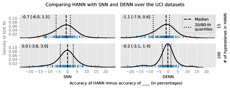
Figure 6: Each blue tick above the x-axis represents a single dataset, where the x-coordinate of the tick is the difference of the accuracy of HANN and either SNN (left) or DENN (right) on the dataset. The number of hyperplanes used by HANN is either 15 (top) or 100 (bottom). The quantities shown in the top-left corner of each subplot are the median, 20-th and 80-th quantiles of the differences, respectively, rounded to 1 decimal place.

Implicit bias for low complexity decision boundary. In Figure 7, we show additional results ran with the same setting for the moons synthetic dataset as in the Empirical Results section. From the perspective of the training loss, the label assignment in the bold-boundary regions is irrelevant. Nevertheless, the optimization consistently appears to be biased toward the geometrically simpler classifier, despite the capacity for fitting complex classifiers.

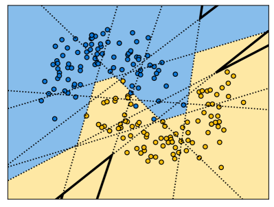
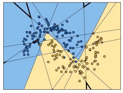
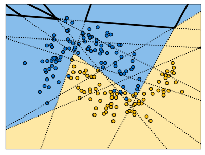
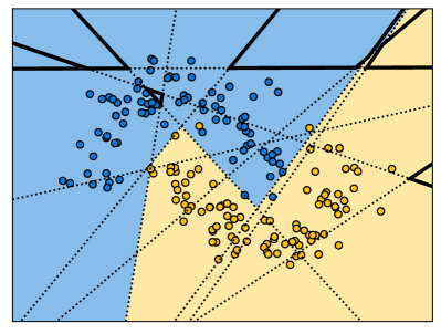
Figure 7: Four independent runs of HANN on the moons synthetic dataset. Data points (circles) drawn from make_moons in sklearn colored by ground truth labels. The hyperplane arrangement is denoted by dotted lines. Coloring of the cells corresponds to the decision region of the trained classifier. A cell $\mathcal{C}$ is highlighted by bold boundaries if 1) no training data lies in $\mathcal{C}$ and 2) $\mathcal{C}$ does not touch the decision boundary.

Appendix D Table of accuracies

Below is the table of accuracies used to make Figure 4. Available as a csv file here: https://github.com/YutongWangUMich/HANN/blob/main/accuracy_table.csv

DSName	HANN15	HANN100	SNN	DENN
abalone	63.41	65.13	66.57	66.38
acute-inflammation	100.00	100.00	100.00	100.00
acute-nephritis	100.00	100.00	100.00	100.00
adult	84.32	85.04	84.76	84.80
annealing	47.00	74.00	76.00	75.00
arrhythmia	62.83	64.60	65.49	67.26
audiology-std	56.00	68.00	80.00	76.00
balance-scale	92.95	96.79	92.31	98.08
balloons	100.00	100.00	100.00	100.00
bank	88.50	88.05	89.03	89.65
blood	75.94	75.40	77.01	73.26
breast-cancer	70.42	63.38	71.83	69.01
breast-cancer-wisc	97.71	98.29	97.14	97.71
breast-cancer-wisc-diag	97.89	98.59	97.89	98.59
breast-cancer-wisc-prog	73.47	71.43	67.35	71.43
breast-tissue	61.54	80.77	73.08	65.38
car	98.84	100.00	98.38	98.84
cardiotocography-10clases	78.91	82.11	83.99	82.30
cardiotocography-3clases	90.58	93.97	91.53	94.35
chess-krvk	47.75	72.77	88.05	80.41
chess-krvkp	98.62	99.37	99.12	99.62
congressional-voting	61.47	57.80	61.47	57.80
conn-bench-sonar-mines-rocks	78.85	84.62	78.85	82.69
conn-bench-vowel-deterding	89.39	98.92	99.57	99.35
connect-4	78.96	86.39	88.07	86.46
contrac	52.72	49.73	51.90	54.89
credit-approval	81.98	79.65	84.30	82.56
cylinder-bands	69.53	73.44	72.66	78.12
dermatology	98.90	97.80	92.31	97.80
echocardiogram	84.85	87.88	81.82	87.88
ecoli	86.90	84.52	89.29	85.71
energy-y1	93.23	97.40	95.83	95.83
energy-y2	89.06	91.15	90.63	90.62
fertility	92.00	92.00	92.00	88.00
flags	39.58	50.00	45.83	52.08
glass	77.36	60.38	73.58	60.38
haberman-survival	72.37	65.79	73.68	65.79
hayes-roth	71.43	82.14	67.86	85.71
heart-cleveland	53.95	59.21	61.84	57.89
heart-hungarian	72.60	79.45	79.45	78.08
heart-switzerland	45.16	51.61	35.48	48.39
heart-va	36.00	30.00	36.00	32.00
hepatitis	82.05	82.05	76.92	79.49
hill-valley	66.83	68.81	52.48	54.62
horse-colic	80.88	83.82	80.88	82.35
ilpd-indian-liver	70.55	69.18	69.86	71.92
image-segmentation	87.76	90.57	91.14	90.57
ionosphere	89.77	87.50	88.64	96.59
iris	100.00	97.30	97.30	100.00
led-display	73.60	75.20	76.40	76.00
lenses	50.00	66.67	66.67	66.67
letter	81.82	96.86	97.26	96.20
libras	64.44	81.11	78.89	77.78
low-res-spect	86.47	90.23	85.71	90.23
lung-cancer	37.50	62.50	62.50	62.50
lymphography	89.19	94.59	91.89	94.59
magic	86.52	87.49	86.92	86.81
mammographic	81.25	80.00	82.50	80.83
molec-biol-promoter	73.08	80.77	84.62	88.46
molec-biol-splice	79.05	78.04	90.09	85.45
monks-1	65.97	69.91	75.23	81.71
monks-2	66.20	66.44	59.26	65.05
monks-3	54.63	61.81	60.42	80.09
mushroom	100.00	100.00	100.00	100.00
musk-1	77.31	84.87	87.39	89.92
musk-2	97.21	98.61	98.91	99.27
nursery	99.75	99.91	99.78	100.00
oocytes-merluccius-nucleus-4d	86.27	83.14	82.35	83.92
oocytes-merluccius-states-2f	92.16	92.55	95.29	92.94
oocytes-trisopterus-nucleus-2f	81.14	82.02	79.82	82.46
oocytes-trisopterus-states-5b	93.86	96.05	93.42	94.74
optical	93.10	95.94	97.11	96.38
ozone	96.53	95.58	97.00	97.48
page-blocks	96.49	96.13	95.83	96.13
parkinsons	87.76	89.80	89.80	85.71
pendigits	94.40	97.11	97.06	97.37
pima	71.88	73.44	75.52	69.79
pittsburg-bridges-MATERIAL	88.46	92.31	88.46	92.31
pittsburg-bridges-REL-L	76.92	73.08	69.23	73.08
pittsburg-bridges-SPAN	60.87	69.57	69.57	73.91
pittsburg-bridges-T-OR-D	84.00	84.00	84.00	84.00
pittsburg-bridges-TYPE	65.38	65.38	65.38	57.69
planning	66.67	55.56	68.89	60.00
plant-margin	50.50	79.50	81.25	83.25
plant-shape	39.00	66.50	72.75	72.50
plant-texture	51.75	75.25	81.25	81.00
post-operative	40.91	63.64	72.73	68.18
primary-tumor	54.88	47.56	52.44	53.66
ringnorm	90.43	85.35	97.51	97.57
seeds	92.31	96.15	88.46	92.31
semeion	74.37	92.71	91.96	96.73
soybean	77.93	88.83	85.11	88.03
spambase	93.57	94.17	94.09	94.87
spect	62.90	63.44	63.98	62.37
spectf	91.98	91.98	49.73	89.30
statlog-australian-credit	65.12	63.37	59.88	61.05
statlog-german-credit	72.40	72.40	75.60	72.00
statlog-heart	85.07	91.04	92.54	92.54
statlog-image	95.15	96.88	95.49	97.75
statlog-landsat	87.55	89.25	91.00	89.90
statlog-shuttle	99.92	99.92	99.90	99.91
statlog-vehicle	78.67	77.25	80.09	81.04
steel-plates	73.61	76.49	78.35	77.53
synthetic-control	94.00	98.00	98.67	99.33
teaching	57.89	57.89	50.00	57.89
thyroid	98.37	98.25	98.16	98.22
tic-tac-toe	96.65	97.07	96.65	98.33
titanic	78.73	78.73	78.36	78.73
trains	100.00	50.00	NaN	NaN
twonorm	97.30	98.27	98.05	98.16
vertebral-column-2clases	88.31	85.71	83.12	85.71
vertebral-column-3clases	81.82	80.52	83.12	80.52
wall-following	92.45	94.79	90.98	91.86
waveform	85.84	84.00	84.80	83.92
waveform-noise	84.72	84.96	86.08	84.32
wine	97.73	100.00	97.73	100.00
wine-quality-red	62.50	65.00	63.00	63.50
wine-quality-white	54.82	61.03	63.73	62.25
yeast	59.03	60.65	63.07	58.22
zoo	96.00	96.00	92.00	100.00

References

- Abadi et al. (2016) Martín Abadi, Ashish Agarwal, Paul Barham, Eugene Brevdo, Zhifeng Chen, Craig Citro, Greg S. Corrado, Andy Davis, Jeffrey Dean, Matthieu Devin, Sanjay Ghemawat, Ian Goodfellow, Andrew Harp, Geoffrey Irving, Michael Isard, Yangqing Jia, Rafal Jozefowicz, Lukasz Kaiser, Manjunath Kudlur, Josh Levenberg, Dan Mane, Rajat Monga, Sherry Moore, Derek Murray, Chris Olah, Mike Schuster, Jonathon Shlens, Benoit Steiner, Ilya Sutskever, Kunal Talwar, Paul Tucker, Vincent Vanhoucke, Vijay Vasudevan, Fernanda Viegas, Oriol Vinyals, Pete Warden, Martin Wattenberg, Martin Wicke, Yuan Yu, and Xiaoqiang Zheng. TensorFlow: A system for large-scale machine learning. In 12th USENIX symposium on operating systems design and implementation (OSDI 16), pp. 265–283, 2016.
- Arora et al. (2019) Sanjeev Arora, Simon S Du, Zhiyuan Li, Ruslan Salakhutdinov, Ruosong Wang, and Dingli Yu. Harnessing the power of infinitely wide deep nets on small-data tasks. In International Conference on Learning Representations, 2019.
- Ashtiani et al. (2020) Hassan Ashtiani, Shai Ben-David, Nicholas JA Harvey, Christopher Liaw, Abbas Mehrabian, and Yaniv Plan. Near-optimal sample complexity bounds for robust learning of Gaussian mixtures via compression schemes. Journal of the ACM (JACM), 67(6):1–42, 2020.
- Audibert & Tsybakov (2007) Jean-Yves Audibert and Alexandre B Tsybakov. Fast learning rates for plug-in classifiers. The Annals of Statistics, 35(2):608–633, 2007.
- Baldi & Vershynin (2019) Pierre Baldi and Roman Vershynin. The capacity of feedforward neural networks. Neural networks, 116:288–311, 2019.
- Bartlett et al. (2017) Peter L Bartlett, Dylan J Foster, and Matus Telgarsky. Spectrally-normalized margin bounds for neural networks. In Proceedings of the 31st International Conference on Neural Information Processing Systems, pp. 6241–6250, 2017.
- Bartlett et al. (2019) Peter L Bartlett, Nick Harvey, Christopher Liaw, and Abbas Mehrabian. Nearly-tight VC-dimension and pseudodimension bounds for piecewise linear neural networks. Journal of Machine Learning Research, 20(63):1–17, 2019.
- Bartlett et al. (2020) Peter L Bartlett, Philip M Long, Gábor Lugosi, and Alexander Tsigler. Benign overfitting in linear regression. Proceedings of the National Academy of Sciences, 117(48):30063–30070, 2020.
- Bartlett et al. (2021) Peter L Bartlett, Andrea Montanari, and Alexander Rakhlin. Deep learning: a statistical viewpoint. Acta Numerica, 2021.
- Baum & Haussler (1989) Eric B Baum and David Haussler. What size net gives valid generalization? Neural computation, 1(1):151–160, 1989.
- Belkin et al. (2018) Mikhail Belkin, Siyuan Ma, and Soumik Mandal. To understand deep learning we need to understand kernel learning. In International Conference on Machine Learning, pp. 541–549, 2018.
- Blumenfeld et al. (2019) Yaniv Blumenfeld, Dar Gilboa, and Daniel Soudry. A mean field theory of quantized deep networks: The quantization-depth trade-off. In Advances in Neural Information Processing Systems, volume 32, 2019.
- Bousquet et al. (2020) Olivier Bousquet, Steve Hanneke, Shay Moran, and Nikita Zhivotovskiy. Proper learning, Helly number, and an optimal SVM bound. In Conference on Learning Theory, 2020.
- Buck (1943) Robert Creighton Buck. Partition of space. The American Mathematical Monthly, 50(9):541–544, 1943.
- Cai et al. (2017) Zhaowei Cai, Xiaodong He, Jian Sun, and Nuno Vasconcelos. Deep learning with low precision by half-wave Gaussian quantization. In Proceedings of the IEEE conference on computer vision and pattern recognition, pp. 5918–5926, 2017.
- Chatterji & Long (2021) Niladri S Chatterji and Philip M Long. Finite-sample analysis of interpolating linear classifiers in the overparameterized regime. Journal of Machine Learning Research, 22(129):1–30, 2021.
- Chizat & Bach (2020) Lenaic Chizat and Francis Bach. Implicit bias of gradient descent for wide two-layer neural networks trained with the logistic loss. In Conference on Learning Theory, pp. 1305–1338. PMLR, 2020.
- Cover (1965) Thomas M Cover. Geometrical and statistical properties of systems of linear inequalities with applications in pattern recognition. IEEE transactions on electronic computers, (3):326–334, 1965.
- Darabi et al. (2019) Sajad Darabi, Mouloud Belbahri, Matthieu Courbariaux, and Vahid Partovi Nia. Regularized binary network training. In Fifth Workshop on Energy Efficient Machine Learning and Cognitive Computing - NeurIPS Edition (EMC2-NIPS), 2019.
- Devroye (1982) Luc Devroye. Any discrimination rule can have an arbitrarily bad probability of error for finite sample size. IEEE Transactions on Pattern Analysis and Machine Intelligence, (2):154–157, 1982.
- Dziugaite & Roy (2017) Gintare Karolina Dziugaite and Daniel M Roy. Computing nonvacuous generalization bounds for deep (stochastic) neural networks with many more parameters than training data. arXiv preprint arXiv:1703.11008, 2017.
- Faragó & Lugosi (1993) András Faragó and Gábor Lugosi. Strong universal consistency of neural network classifiers. IEEE Transactions on Information Theory, 39(4):1146–1151, 1993.
- Floyd & Warmuth (1995) Sally Floyd and Manfred Warmuth. Sample compression, learnability, and the Vapnik-Chervonenkis dimension. Machine learning, 21(3):269–304, 1995.
- Fukuda (2015) Komei Fukuda. Lecture: Polyhedral computation, Spring 2013, 2015. URL http://www-oldurls.inf.ethz.ch/personal/fukudak/lect/pclect/notes2015/PolyComp2015.pdf.
- Geiger & Team (2020) Lukas Geiger and Plumerai Team. Larq: An open-source library for training binarized neural networks. Journal of Open Source Software, 5(45):1746, January 2020.
- Goodfellow et al. (2016) Ian Goodfellow, Yoshua Bengio, and Aaron Courville. Deep learning. MIT press, 2016.
- Gunasekar et al. (2018) Suriya Gunasekar, Jason Lee, Daniel Soudry, and Nathan Srebro. Implicit bias of gradient descent on linear convolutional networks. In Advances in Neural Information Processing Systems, 2018.
- Györfi et al. (2006) László Györfi, Michael Kohler, Adam Krzyzak, and Harro Walk. A distribution-free theory of nonparametric regression. Springer Science & Business Media, 2006.
- Hanneke & Kontorovich (2021) Steve Hanneke and Aryeh Kontorovich. Stable sample compression schemes: New applications and an optimal SVM margin bound. In Algorithmic Learning Theory, pp. 697–721. PMLR, 2021.
- Hanneke et al. (2019) Steve Hanneke, Aryeh Kontorovich, and Menachem Sadigurschi. Sample compression for real-valued learners. In Algorithmic Learning Theory, pp. 466–488. PMLR, 2019.
- He et al. (2016) Kaiming He, Xiangyu Zhang, Shaoqing Ren, and Jian Sun. Deep residual learning for image recognition. In Proceedings of the IEEE conference on computer vision and pattern recognition, pp. 770–778, 2016.
- Hinton et al. (2012) Geoffrey Hinton, Nitsh Srivastava, and Kevin Swersky. Neural networks for machine learning. Coursera, video lectures, 264(1):2146–2153, 2012.
- Hubara et al. (2017) Itay Hubara, Matthieu Courbariaux, Daniel Soudry, Ran El-Yaniv, and Yoshua Bengio. Quantized neural networks: Training neural networks with low precision weights and activations. The Journal of Machine Learning Research, 18(1):6869–6898, 2017.
- Kim et al. (2019) Hyungjun Kim, Kyungsu Kim, Jinseok Kim, and Jae-Joon Kim. Binaryduo: Reducing gradient mismatch in binary activation network by coupling binary activations. In International Conference on Learning Representations, 2019.
- Kim et al. (2021) Yongdai Kim, Ilsang Ohn, and Dongha Kim. Fast convergence rates of deep neural networks for classification. Neural Networks, 138:179–197, 2021.
- Klambauer et al. (2017) Günter Klambauer, Thomas Unterthiner, Andreas Mayr, and Sepp Hochreiter. Self-normalizing neural networks. In Advances in Neural Information Processing Systems, pp. 971–980, 2017.
- Kohler & Langer (2020) Michael Kohler and Sophie Langer. On the rate of convergence of fully connected deep neural network regression estimates. arXiv preprint arXiv:1908.11133, 2020.
- Langer (2021) Sophie Langer. Analysis of the rate of convergence of fully connected deep neural network regression estimates with smooth activation function. Journal of Multivariate Analysis, 182:104695, 2021.
- Li et al. (2017) Hao Li, Soham De, Zheng Xu, Christoph Studer, Hanan Samet, and Tom Goldstein. Training quantized nets: A deeper understanding. In Proceedings of the 31st International Conference on Neural Information Processing Systems, pp. 5813–5823, 2017.
- Lin et al. (2018) Ji Lin, Chuang Gan, and Song Han. Defensive quantization: When efficiency meets robustness. In International Conference on Learning Representations, 2018.
- Lin et al. (2017) Xiaofan Lin, Cong Zhao, and Wei Pan. Towards accurate binary convolutional neural network. Advances in Neural Information Processing Systems, 30, 2017.
- Littlestone & Warmuth (1986) Nick Littlestone and Manfred Warmuth. Relating data compression and learnability. 1986.
- Lovász & Plummer (2009) László Lovász and Michael D Plummer. Matching theory, volume 367. American Mathematical Soc., 2009.
- Maass (1994) Wolfgang Maass. Neural nets with superlinear VC-dimension. Neural Computation, 6(5):877–884, 1994.
- Mishra et al. (2018) Asit Mishra, Eriko Nurvitadhi, Jeffrey J Cook, and Debbie Marr. WRPN: Wide reduced-precision networks. In International Conference on Learning Representations, 2018.
- Moran & Yehudayoff (2016) Shay Moran and Amir Yehudayoff. Sample compression schemes for VC classes. Journal of the ACM (JACM), 63(3):1–10, 2016.
- Mukherjee & Basu (2017) Anirbit Mukherjee and Amitabh Basu. Lower bounds over Boolean inputs for deep neural networks with ReLU gates. arXiv preprint arXiv:1711.03073, 2017.
- Nagarajan & Kolter (2019) Vaishnavh Nagarajan and J Zico Kolter. Uniform convergence may be unable to explain generalization in deep learning. In Advances in Neural Information Processing Systems, 2019.
- Naslund (2017) Eric Naslund. Compression and VC-dimension. Lecture notes for COS 598, Unsupervised Learning: Theory and Practice, 2017.
- Neyshabur et al. (2017) Behnam Neyshabur, Srinadh Bhojanapalli, David McAllester, and Nathan Srebro. Exploring generalization in deep learning. In Proceedings of the 31st International Conference on Neural Information Processing Systems, pp. 5949–5958, 2017.
- Qin et al. (2020) Haotong Qin, Ruihao Gong, Xianglong Liu, Xiao Bai, Jingkuan Song, and Nicu Sebe. Binary neural networks: A survey. Pattern Recognition, 105:107281, 2020.
- Rastegari et al. (2016) Mohammad Rastegari, Vicente Ordonez, Joseph Redmon, and Ali Farhadi. XOR-Net: Imagenet classification using binary convolutional neural networks. In European conference on computer vision, pp. 525–542. Springer, 2016.
- Schapire (2013) Robert E Schapire. Explaining AdaBoost. In Empirical inference, pp. 37–52. Springer, 2013.
- Schmidt-Hieber (2020) Johannes Schmidt-Hieber. Nonparametric regression using deep neural networks with ReLU activation function. Annals of Statistics, 48(4):1875–1897, 2020.
- Shalev-Shwartz & Ben-David (2014) Shai Shalev-Shwartz and Shai Ben-David. Understanding machine learning: From theory to algorithms. Cambridge university press, 2014.
- Shankar et al. (2020) Vaishaal Shankar, Alex Fang, Wenshuo Guo, Sara Fridovich-Keil, Jonathan Ragan-Kelley, Ludwig Schmidt, and Benjamin Recht. Neural kernels without tangents. In International Conference on Machine Learning, pp. 8614–8623. PMLR, 2020.
- Vapnik & Chervonenkis (1971) VN Vapnik and A Ya Chervonenkis. On the uniform convergence of relative frequencies of events to their probabilities. Measures of Complexity, 16(2):11, 1971.
- Vershynin (2020) Roman Vershynin. Memory capacity of neural networks with threshold and rectified linear unit activations. SIAM Journal on Mathematics of Data Science, 2(4):1004–1033, 2020.
- Wu et al. (2018) Xundong Wu, Xiangwen Liu, Wei Li, and Qing Wu. Improved expressivity through dendritic neural networks. In Proceedings of the 32nd International Conference on Neural Information Processing Systems, pp. 8068–8079, 2018.
- Wyner et al. (2017) Abraham J Wyner, Matthew Olson, Justin Bleich, and David Mease. Explaining the success of AdaBoost and random forests as interpolating classifiers. The Journal of Machine Learning Research, 18(1):1558–1590, 2017.
- Yin et al. (2019) Penghang Yin, Jiancheng Lyu, Shuai Zhang, Stanley Osher, Yingyong Qi, and Jack Xin. Understanding straight-through estimator in training activation quantized neural nets. In International Conference on Learning Representations, 2019.
- Zhang et al. (2021) Chiyuan Zhang, Samy Bengio, Moritz Hardt, Benjamin Recht, and Oriol Vinyals. Understanding deep learning (still) requires rethinking generalization. Communications of the ACM, 64(3):107–115, 2021.