Space-time approach to spontaneous symmetry breaking in the Abelian-gauge interaction

Abstract

Spontaneous symmetry breaking is studied by regarding it as a phenomenon in the eternal intermediate state due to sequential perturbations. The concept of the relativistic many-body state is applied to this intermediate state ocurring in the collision of massless Dirac fermions. Time in the relativistic many-body state should evolve while maintaining the direction of time in each particle, even if the particle are viewed from any inertial frames. This kinematical requirement leads to spontaneous symmetry breaking in the vacuum of these states, which gives a different meaning to the results of the Higgs model. In this vacuum, massless fermion-antifermion pairs and coherent collection of gauge bosons condense, which determine each other’s mass. When a local excitation of the condensed gauge bosons propagates in space, a Higgs-like boson appears. The effective coupling of this Higgs-like boson to gauge bosons is calculated as a one-loop process. With this coupling, the total cross section of the pair annihilation of fermion and antifermion to gauge boson pair is calculated. Renormalizability of this model is discussed using the inductive method. Since the Higgs Lagrangian is not assumed, the divergence we must renormalize is only the logarithmic divergence, not the quadratic one.

I Introduction

Spontaneous symmetry breaking is examined using a vector Abelian-gauge field $B_{\mu}$ coupled to massless Dirac fermi field $\varphi$

$$L_{0}(x)=-\frac{1}{4}F^{\mu\nu}F_{\mu\nu}+\bar{\varphi}(i\partial_{\mu}+gB_{\mu})\gamma^{\mu}\varphi.$$ (1)

In the usual form of quantum relativistic field theory, the world is modeled as the physical process that connects initial and final asymptotic states of the particle collision. The Fock state created on the free vacuum is used for this asymptotic state. This Fock state exists only when all interactions are switched off, and this is a good approximation in the case of short-range interaction. However, spontaneous symmetry breaking occurs in situations where the gauge field that causes long-range forces is still an extended object. Therefore, the interaction is not switched off even in the initial and final asymptotic states. This is a reason why the Fock state is unsuitable for deriving spontaneous symmetry breaking. In the case of long-range forces, there is always an interaction between the particles, and in this case the more natural point of view is as follows. The real world is modeled as an eternal intermediate state due to sequential perturbations [1]. We are in the middle of such intermediate states, where the broken-symmetry vacuum is expected to appear. Consider an intermediate state as shown in Figure.1 caused by the collision of massless Dirac fermion. In order to obtain a broken-symmetry vacuum, we must think of a suitable representation of states.

In quantum field theory with infinite degrees of freedom, there are countless inequivalent representations with the same commutation relations in a free vacuum, but belonging to different Hilbert spaces [2] [3] [4] [5]. The choice of representation must follow natural phenomena, but the form of representation is decided by the human side.

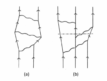
Figure 1: Examples of (a) two-body intermediate states (b) three-body intermediate states.

For the suitable representation of the broken-symmetry vacuum, let us apply the concept of relativistic many-body state to this intermediate state [6]. There is an assumption about the form taken by the many-body states: Time in the many-body state should evolve while maintaining the direction of time in each particle, even if particles are viewed from any observer When it is applied to the intermediate states, time in the relativistic many-body state should evolve while maintaining the direction of time in each particle, even if particles in the intermediate states are viewed from any inertial frame. As long as it is a one-particle state, this is merely a matter of interpretation. However, in the many-body state, it becomes a serious problem. If this is not followed, there will be an object coming from the future to the present in the many-body state, and its relation to other objects coming from the past cannot be explained. In this case, the many-body state will be chaotic. The relationship between different objects is understood on the premise that they follow a common direction of time [7]. In the intermediate state, although particles travel not only time-like paths but also space-like ones, the temporal order of events should not be reversed. This criterion should give an inequivalent representations with a suitable form. However, in the relativistic many-body state, there is a situation that threatens this.

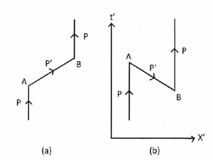
Figure 2: (a) The motion of a massless Dirac fermion perturbed by $U_{1}$ and $U_{2}$ at $A$ and $B$ ($t_{2}>t_{1}$). (b) When viewed from a fast-moving inertial frame $(x^{\prime},t^{\prime})$, the order of two events separated by spacelike interval is reversed ($t^{\prime}_{2}<t^{\prime}_{1}$).

Consider the second-order perturbation process of a moving massless Dirac fermion under disturbances in Figure.2(a). There are two disturbances, $U_{1}$ in $A$ at a time $t_{1}$, and $U_{2}$ in $B$ at a later time $t_{2}$, in which the second disturbance $U_{2}$ restore the fermion to its original state with a momentum $p$. Such an amplitude is calculated by summing all possible, timelike or spacelike, intermediate states between $A$ and $B$ over their momenta $\mbox{\boldmath$p$}^{\prime}$ viewed from different inertial frame (see Appendix.A). The states on the path $AB$ look different when viewd from other inertial systems. In the inertial system of a coordinate $(\mbox{\boldmath$x$},t)$, a fermion with a negative electric charge and momentum $p$ leave $A$ at $x_{1}$ and $t_{1}$, and reach $B$ at $x_{2}$ and $t_{2}(>t_{1})$. When this motion is viewed from another inertial system moving in the $x$-direction at a relative velocity $v$ to the original one, it follows a Lorentz transformation to a new coordinates $(\mbox{\boldmath$x^{\prime}$},t^{\prime})$. The time difference $t_{2}-t_{1}$ between $A$ and $B$ is Lorentz transformed to

$$t_{2}^{\prime}-t_{1}^{\prime}=\frac{1}{\sqrt{1-(v/c)^{2}}}\left[t_{2}-t_{1}-\frac{v}{c^{2}}(x_{2}-x_{1})\right].$$ (2)

A prominent feature of the Lorentz transformation is that it does not leave the temporal order of events on the spacelike path invariant. When the fermion has a small velocity, the observer has more options for having a large relative velocity $v$ to the fermion. A sufficiently large spacelike interval between two events, such as $c(t_{2}-t_{1})<(v/c)(x_{2}-x_{1})$ in Eq.(2), reverses the temporal order of two events, $t_{2}^{\prime}<t_{1}^{\prime}$ as shown in Figure.2(b).

The natural interpretation without the reversal of temporal order is that a positively-charged antifermion runs in the opposite direction. (Historically, Stueckelberg first stressed this [8], and later Feynman independently made an intuitive explanation for the raison d’etre of antiparticle along this line [9].) The intermediate many-body state should be described using antifermion so that the time direction is not reversed by any observer. Therein lies the key for understanding the vacuum with broken-chiral-symmetry.

In this paper, we derive spontaneous symmetry breaking from a kinematical requirement. In Section 2, using the massless fermion system coupled to the Abelian-gauge field, the concept of the relativistic many-body state is applied to the intermediate states in the collision of this system, and it is shown that the kinematical requirement on the time direction in this many-body state leads to the physical vacuum with broken-chiral-symmetry. Section 3 describes some dynamical consequences of this kinematical requirement. In Section 3-1, and 3-2, the mass of the fermion is generated from gauge bosons in the condensed field energy. In Section 3-3, the mass generation of the gauge boson in the physical vacuum is explained. In Section 3-4, the Higgs-like boson is derived as a local excitation propagating in the physical vacuum, the mass of which is calculated as an excitation energy. Section 4 gives an interim summary. In Section 5, one-loop perturbation calculation is performed for the effective coupling of the Higgs-like mode to the gauge field, and for the self interaction of this mode. In Section 6, the total cross section is calculated for the pair-annihilation of massive fermion and antifermon to massive gauge bosons. In Section 7, renormalizability of this model is examined. In Section 8, some generalization to the electroweak interaction is briefly discussed.

II Relativistic many-body states of massless Dirac fermions

As an example of the relativistic many-body state, consider the intermediate state in the direct scattering of two massless Dirac fermions, and regard it as a two-body state. Figure.3 shows its fourth-order process. The particle in the intermediate state (thick lines with arrows) looks a normal or time-reversed one, depending on what inertial frame it is viewed from. Hence four different combinations of the temporal order appear in the two-body state [10] (The exchange scattering is also possible, in which the gauge-boson lines are crossed at the left and right ends of Figure.3, and not crossed elsewhere.) The non-relativistic two-body state contains only the left end of Figure.3, whereas the relativistic two-body state is a superposition of all possible combinations. To regard the relativistic intermediate state as the many-body state, no matter what form an individual particle takes, time should evolve in the same direction there no matter what inertial frames they are viewed from. Hence, these time-reversed motions should be interpreted as the motion of antifermion. All processes in Figure.3, the propagation of massless fermion, the pair creation and annihilation of massless fermion and antifermion, occur in the common direction of time.

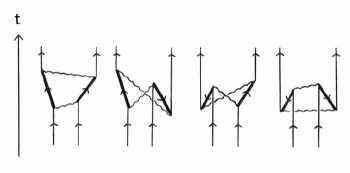
Figure 3: The relativistic two-body states appearing in the intermediate state of massless fermions (thick lines with arrows). Four types of combination appear on the temporal order of two fermions, if antifermion is not introduced.

Each vertex in Figure.3 has two possibilities, a vertex of massless fermion or that of antifermion. To obtain the representation which is always valid when viewed from any reference frame, combine two pictures in Figure.2. Momentum, electric charge and spin, which prescribe all properties of massless fermion, are not positive definite, and therefore the operation of $a^{s}(\mbox{\boldmath$p$})$ on the state can be equated with that of $b^{s\dagger}(-\mbox{\boldmath$p$})$. We define a new annihilation operator at $A$ in Figure.2 by considering a superposition of $a^{s}(\mbox{\boldmath$p$})$ and $b^{s\dagger}(-\mbox{\boldmath$p$})$

$$A^{s}(\mbox{\boldmath$p$})=\cos\theta_{\mbox{\boldmath$p$}}a^{s}(\mbox{\boldmath$p$})+\sin\theta_{\mbox{\boldmath$p$}}b^{s\dagger}(-\mbox{\boldmath$p$}).$$ (3)

In contrast, if $a^{s}(\mbox{\boldmath$p$})$ and $b^{s\dagger}(-\mbox{\boldmath$p$})$ represent massive fermion, they have different meaning to the state because mass is positive definite, and their superposition cannot be considered. Hence, this superposition is characteristic of massless fermion before symmetry breaking.

Let us assign a parameter to each inertial reference frame in which antifermions are necessary to protect the temporal order. The volume of such a parameter space is reflected in $\sin\theta_{\mbox{\boldmath$p$}}$ in Eq.(3). Physically, this $\theta_{\mbox{\boldmath$p$}}$ comes from the interaction of fermions with the gauge field, but regardless of its details, the following is expected. When $\mbox{\boldmath$p$}=0$, the difference in momentum between $a^{s}(\mbox{\boldmath$p$})$ and $b^{s\dagger}(-\mbox{\boldmath$p$})$ disappears. Therefore, the probability of finding the above inertial frames is maximized, suggesting $\cos\theta_{\mbox{\boldmath$p$}}=\sin\theta_{\mbox{\boldmath$p$}}$. When $\mbox{\boldmath$p$}^{2}\rightarrow\infty$, no such inertial frame can be found, and $\sin\theta_{\mbox{\boldmath$p$}}\rightarrow 0$ is expected. Furthermore, when the coupling $g$ to gauge field disappears, there is no reason to consider the many-body state, then $\sin\theta_{\mbox{\boldmath$p$}}=0$ is required. The same interpretation is possible also for the event at $B$ in Figure.2. A new annihilation operator $B^{s}(-\mbox{\boldmath$p$})$ is defined as a superposition of the annihilation $b^{s}(-\mbox{\boldmath$p$})$ of massless antifermion in Figure.2(b), and the creation $a^{s\dagger}(\mbox{\boldmath$p$})$ of massless fermion in 2(a)

$$B^{s}(-\mbox{\boldmath$p$})=\cos\theta_{\mbox{\boldmath$p$}}b^{s}(-\mbox{\boldmath$p$})-\sin\theta_{\mbox{\boldmath$p$}}a^{s\dagger}(\mbox{\boldmath$p$}).$$ (4)

This $B^{s}(-\mbox{\boldmath$p$})$ is orthogonal to $A^{s}(-\mbox{\boldmath$p$})$ [11]. These $A^{s}(\mbox{\boldmath$p$}^{\prime})$ and $B^{s}(-\mbox{\boldmath$p$}^{\prime})$ describe not only the two-body state, but also general many-body states. These superposed operators define the lowest-energy state $|\widetilde{0}\rangle$ by imposing $A^{s}(\mbox{\boldmath$p$})|\widetilde{0}\rangle=B^{s}(-\mbox{\boldmath$p$})|\widetilde{0}\rangle=0$ on it [12] This lowest-energy state $|\widetilde{0}\rangle$ should have a Lorentz-invariant form, and is called physical vacuum. The cyclicity of vacuum is also expected for this particular vacuum belonging to a particular Hilbert space.

II.1 Physical vacuum

The explicit form of $|\widetilde{0}\rangle$ is inferred as follows. In the case of massless fermions with velocity close to the velocity of light, $\cos\theta_{\mbox{\boldmath$p$}}\rightarrow 1$ is required, and the physical vacuum agrees with the free vacuum. Therefore $|\widetilde{0}\rangle$ includes $\cos\theta_{\mbox{\boldmath$p$}}|0\rangle$. Conversely, in the case of massless fermions with small momentum, various inertial frames with large relative velocity $v$ can be set so that it satisfies $t_{2}^{\prime}-t_{1}^{\prime}<0$ in Eq.(2). Therefore, massless fermions and antifrmions are required in $|\widetilde{0}\rangle$, which leads to $b^{s\dagger}(-\mbox{\boldmath$p$})a^{s\dagger}(\mbox{\boldmath$p$})|0\rangle$. The simplest possible form of $|\widetilde{0}\rangle$ is a superpositions of $\cos\theta_{\mbox{\boldmath$p$}}|0\rangle$ and $\sin\theta_{\mbox{\boldmath$p$}}b^{s\dagger}(-\mbox{\boldmath$p$})a^{s\dagger}(\mbox{\boldmath$p$})|0\rangle$. Such a superposition is possible for all $p$, and $|\widetilde{0}\rangle$ is the product of these superpositions (see Appendx.B)

$$|\widetilde{0}\rangle=\prod_{p,s}\left[\cos\theta_{\mbox{\boldmath$p$}}+\sin\theta_{\mbox{\boldmath$p$}}b^{s\dagger}(-\mbox{\boldmath$p$})a^{s\dagger}(\mbox{\boldmath$p$})\right]|0\rangle.$$ (5)

When the suitable form for the relativistic many-body states is required, broken-symmetry vacuum manifests itself in the lowest-energy state of the intermediate states of the massless Dirac fermions. (The real particle in $A^{s\dagger}(\mbox{\boldmath$p$})|\widetilde{0}\rangle$ or $B^{s\dagger}(\mbox{\boldmath$p$})|\widetilde{0}\rangle$ is an objective existence common to all observers, and follows the Lorentz transformation, whereas the massless particle in $|\widetilde{0}\rangle$ is not such an existence. In this sense, the Lorentz transformation which connects different observers does not apply to the latter, and $|\widetilde{0}\rangle$ is Lorentz invariant.) (This $|\widetilde{0}\rangle$ was first introduced to elementary-particle physics by [13] in analogy with superconductivity [11]. The above derivation shows that it does not depend on the attractive interaction, but has generality that it depends only on the kinematical requirement.)

II.2 Pair annihilation of maassless fermion-antifermion pairs to gauge boson

The broken-symmetry vacuum does not end only with the creation of fermion and antifermion. Due to $\bar{\varphi}(i\partial_{\mu}+gB_{\mu})\gamma^{\mu}\varphi$, the massless fermion-antifermion pair with opposite momentum in Eq.(5) annihilate to a gauge boson with a 4-momentum $(2p_{0},\mbox{\boldmath$0$})$ in the center-of-mass frame of the pair, and this gauge boson annihilates to other massless fermion-antifermion pair in $|\widetilde{0}\rangle$. Such a $s$-channel process between massless objects possesses no threshold energy, and it results in an equilibrium state between the massless fermion-antifermion pairs and the gauge bosons. At each point in space, the total field-energy of the $U(1)$ gauge field $B_{\mu}$

$$\int T^{00}(x)d^{3}x=\frac{1}{4\pi}\int\left(-F^{0\mu}F_{0\mu}+\frac{1}{4}F^{\mu\nu}F_{\mu\nu}\right)d^{3}x\equiv\widehat{\beta},$$ (6)

condenses, which is a coherent collection of gauge bosons created at different points, and is a Lorentz- and gauge-invariant scalar quantity with the dimension of mass. To incorporate such a $\widehat{\beta}$ to $|\widetilde{0}\rangle$, the free vacuum $|0\rangle$ in the right-hand side of Eq.(5) is replaced by a condensed vacuum $|0_{r}\rangle$ satisfying $\langle 0_{r}|\int T_{c}^{00}(x)d^{3}x|0_{r}\rangle\equiv\langle\widehat{\beta}\rangle\neq 0$. This $|0_{r}\rangle$ is the lowest-energy state of the condensed gauge bosons, and its explicit form is to be studied in the future [14]. Here, leaving the explicit form of $|0_{r}\rangle$ aside, Eq.(5) is redefined as follows

$$|\widetilde{0}\rangle=\prod_{p,s}\left[\cos\theta_{\mbox{\boldmath$p$}}+\sin\theta_{\mbox{\boldmath$p$}}e^{i\alpha(x)}b^{s\dagger}(-\mbox{\boldmath$p$})a^{s\dagger}(\mbox{\boldmath$p$})\right]|0_{r}\rangle.$$ (7)

A phase factor $\exp[\alpha(x)]$ with respect to $U(1)$ symmetry appears at each point in space-time [15].

III Dynamical consequences after spontaneous symmetry breaking

The broken-symmetry vacuum $|\widetilde{0}\rangle$ has a kinematical origin, but produces some dynamical consequences. In the Higgs model, symmetry breaking and its consequence are derived by adding

$$L_{h}(x) = |(i\partial_{\mu}+gB_{\mu})(v_{h}+h)|^{2}$$ (8)

$$- \mu^{2}|v_{h}+h|^{2}-\lambda|v_{h}+h|^{4}$$

$$- \frac{m_{f}}{v_{h}}(v_{h}+h)\bar{\varphi}\varphi,$$

to $L_{0}(x)$, where $h=h_{1}+ih_{2}$ [16] [17]. In what follows, we derive the consequences without the help of $L_{h}(x)$, and examine the meaning of parameters in $L_{h}(x)$.

III.1 Pair production of massless fermions

The condensed field-energy $\widehat{\beta}$ in Eq.(6) is a coherent collection of gauge bosons, which can create massless fermion-antifermion pairs. QED has a good example of this, where a strong electric field $E_{\mu}=F_{0,\mu}$ creates massive fermion-antifermion pairs. We know the formula of pair-production rate $\Gamma(E\rightarrow f^{+}f^{-})$ by Schwinger [18]

$$\Gamma(E\rightarrow f^{+}f^{-})=\frac{\alpha E^{2}}{\pi^{2}}\sum_{n=1}^{\infty}\frac{1}{n^{2}}\exp\left(-\frac{n\pi m^{2}}{\alpha E}\right),$$ (9)

where $\alpha=e^{2}/(4\pi)$. In QED, strong electric field is necessary to create massive fermion-antifermion pairs, but such a strong field is not required to create massless fermion-antifermion pairs. Translate this $\Gamma(E\rightarrow f^{+}f^{-})=2Im(L_{EH})$ ($L_{EH}$ is the Euler-Heisenberg Lagrangian [19]) into the situation of $L_{0}(x)$. Replace the macroscopic field-energy density $E^{2}$ in Eq.(9) with $T^{00}_{c}(x)$ of the microscopic field. In our case, all energy of the field is put into the kinetic energy of created massless particles, and therefore $m^{2}$ in Eq.(9) is replaced by $\mbox{\boldmath$p$}^{2}$. Incorporate Eq.(9) into the Lagrangian density representing a states process ($\mbox{\boldmath$p$}^{2}=0$, that is, $m^{2}=0$ in Eq.(9)). The coupling of the massless fermion and antifermion to the condensed field-energy $\widehat{\beta}$ is as follows

$$\bar{\varphi}(x)\left[\frac{g^{2}}{8\pi^{3}}\int T^{00}_{c}(x)d^{3}x\sum^{\infty}_{n=1}\frac{1}{n^{2}}\right]\varphi(x)=\frac{g^{2}}{48\pi}\bar{\varphi}(x)\widehat{\beta}\varphi(x),$$ (10)

(here $\sum_{n=1}^{\infty}n^{-2}=\pi^{2}/6$ is used), which is a simplified $L_{EH}$ of this case.

III.2 Crossing symmetry and fermion’s mass

Crossing symmetry is used to convert the amplitude by Eq.(10) into that of a $t$-channel process between fermi fields. There, the $\widehat{\beta}$ serves as a mean field acting on the fermion and antifermion as follows

$$\bar{\varphi}(x)\left(i/{\!\!\!}{\partial}+\left[\widehat{g}^{2}\widehat{\beta}+gB_{\mu}\gamma^{\mu}\right]\right)\varphi(x),$$ (11)

where $g^{2}/(48\pi)=\widehat{g}^{2}$. The physical vacuum $|\widetilde{0}\rangle$ is a stable state with the lowest-energy. Hence, Eq.(11) sandwiched between $\langle\widetilde{0}|$ and $|\widetilde{0}\rangle$ is diagonal with respect to $A^{s\dagger}(\mbox{\boldmath$p$})A^{s}(\mbox{\boldmath$p$})$ and $B^{s\dagger}(-\mbox{\boldmath$p$})B^{s}(-\mbox{\boldmath$p$})$ for all $p$. The mean field $\widehat{\beta}$ is an average of many degrees of freedom, and therefore it does not easily change through the creation or annihilation of each fermion. Hence, $\widehat{\beta}$ is approximated by a constant vacuum-expectation-value (VEV) $\langle\widetilde{0}|\widehat{\beta}|\widetilde{0}\rangle=\langle\widehat{\beta}\rangle$. Following the same procedure as in [11], using the reverse relation of Eqs.(3) and (4) in Eq.(11), the condition for Eq.(11) to be diagonal is obtained

$$\cos^{2}\theta_{\mbox{\boldmath$p$}} = \frac{1}{2}\left(1+\frac{\epsilon_{p}}{\sqrt{\epsilon_{p}^{2}+(\widehat{g}^{2}\langle\widehat{\beta}\rangle)^{2}}}\right),$$

$$\sin^{2}\theta_{\mbox{\boldmath$p$}} = \frac{1}{2}\left(1-\frac{\epsilon_{p}}{\sqrt{\epsilon_{p}^{2}+(\widehat{g}^{2}\langle\widehat{\beta}\rangle)^{2}}}\right).$$ (12)

This condition satisfies $\cos\theta_{\mbox{\boldmath$p$}}=\sin\theta_{\mbox{\boldmath$p$}}$ at $\mbox{\boldmath$p$}=0$, and $\sin\theta_{\mbox{\boldmath$p$}}\rightarrow 0$ at $\mbox{\boldmath$p$}\rightarrow\infty$ as expected.

The diagonalized form of Eq.(11) includes $\sqrt{\epsilon_{p}^{2}+(\widehat{g}^{2}\langle\widehat{\beta}\rangle)^{2}}\bar{\psi}(p)\psi(p)$, where $\psi(p)$ represents an operator of massive fermion. The fermion’s mass $m_{f}$ arises from the condensed field-energy $\widehat{\beta}$ of the gauge field $B_{\mu}$

$$m_{f}=\widehat{g}^{2}\langle\widehat{\beta}\rangle=\frac{g^{2}}{48\pi}\langle\widetilde{0}|\int T_{c}^{00}(x)d^{3}x|\widetilde{0}\rangle.$$ (13)

This mass comes from the fact that massless antifermions are needed to constitute the relativistic many-body states (This situation parallels the fact in classical physics that $E=c\sqrt{p^{2}+m^{2}c^{2}}$, in which the mass $m$ has its origin, comes from the relativistic relationship between energy and momentum.) This derivation does not depend on whether the effective interaction between massless fermions is attractive or repulsive [20].

III.3 Goldstone mode and massive gauge boson

The physical vacuum $|\widetilde{0}\rangle$ is not a simple system, and therefore the response of $|\widetilde{0}\rangle$ to $B_{\mu}$ involves a non-linear relation. The minimal interaction $L_{0}^{min}(x)=\bar{\varphi}(x)(i\partial_{\mu}+gB_{\mu})\gamma^{\mu}\varphi(x)$ itself changes to an effective one due to the perturbation to $|\widetilde{0}\rangle$ by ${\cal H}_{I}(x)=gj^{\mu}(x)B_{\mu}(x)$. (The perturbation to $|\widetilde{0}\rangle$ by ${\cal H}_{I}(x)$ does not double count the effect, because the physical vacuum $|\widetilde{0}\rangle$ in Eq.(7) does not come from ${\cal H}_{I}(x)$, but is selected for the kinematical reason.) Consider a perturbation expansion of $\int d^{4}xL_{0}^{min}(x)$ in powers of $g$

$$\langle\widetilde{0}|\int d^{4}x_{1}L_{0}^{min}(x_{1})exp\left(i\int{\cal H}_{I}(x_{2})d^{4}x_{2}\right)|\widetilde{0}\rangle$$

$$=\langle\widetilde{0}|\int d^{4}x_{1}\bar{\varphi}(x_{1})\gamma^{\mu}[i\partial_{\mu}+gB_{\mu}(x_{1})]\varphi(x_{1})|\widetilde{0}\rangle$$

$$+\langle\widetilde{0}|\int d^{4}x_{1}L_{0}^{min}(x_{1})ig\int d^{4}x_{2}j^{\nu}(x_{2})B_{\nu}(x_{2})|\widetilde{0}\rangle+\cdots,$$

(1) In the last line of Eq.(LABEL:eq:34), $B_{\nu}(x_{2})$ couples to $\bar{\varphi}(x_{1})i\partial^{\mu}\gamma_{\mu}\varphi(x_{1})$ in $L^{min}_{0}(x_{1})$. Integrate this term partially over $x_{1}$ in $\bar{\varphi}(x_{1})i\partial^{\mu}\gamma_{\mu}\varphi(x_{1})$, and use the fact that $\varphi(x_{1})$ vanishes at $x_{1}\rightarrow\infty$. As a result, two types of terms appear, one including $i\partial^{\mu}\bar{\varphi}(x_{1})\gamma_{\mu}\varphi(x_{1})$, and the other including $\partial^{\mu}|\widetilde{0}\rangle$. Because the physical vacuum $|\widetilde{0}\rangle$ in Eq.(7) has an explicit $x$-dependence in the phase $\alpha(x)$, the integration in Eq.(LABEL:eq:34) extends to this $\alpha(x)$. The latter term is given by

$$g \langle\widetilde{0}|\int d^{4}x_{1}j_{\mu}(x_{1})\int d^{4}x_{2}j^{\nu}(x_{2})B_{\nu}(x_{2})\partial^{\mu}|\widetilde{0}\rangle$$

$$+ g \partial^{\mu}\langle\widetilde{0}|\int d^{4}x_{1}j_{\mu}(x_{1})\int d^{4}x_{2}j^{\nu}(x_{2})B_{\nu}(x_{2})|\widetilde{0}\rangle.$$

Here $\partial^{\mu}|\widetilde{0}\rangle$ is a product of $\partial^{\mu}\alpha(x)$ and $\prod_{p,s}\sin\theta_{\mbox{\boldmath$p$}}e^{i\alpha(x)}b^{s\dagger}(-\mbox{\boldmath$p$})a^{s\dagger}(\mbox{\boldmath$p$})|0_{r}\rangle$. These $x_{1}$ and $x_{2}$ are separated only microscopically in space-time. If we observe this phenomenon from a far distant point, it would appear to be a local phenomenon at $X=(x_{1}+x_{2})/2$. The relative motion along $Y=x_{2}-x_{1}$ is indirectly observed as a coefficient appearing in Eq.(LABEL:eq:374). For the observer at a distant space-time point, it is useful to rewrite $d^{4}x_{1}d^{4}x_{2}$ in Eq.(LABEL:eq:374) to $d^{4}Xd^{4}Y$. The influence of the physical vacuum $|\widetilde{0}\rangle$ appears in Eq.(LABEL:eq:374) through the following coefficient for $\mu=\nu$,

$$m_{B}^{2}=g^{2}\langle\widetilde{0}|\int j_{\mu}(Y)j^{\mu}(0)d^{4}Y|\widetilde{0}\rangle.$$ (16)

With this Lorentz- and gauge-invariant $m_{B}^{2}$, Eq.(LABEL:eq:374) is rewritten as

$$\frac{2i}{g}m^{2}_{B}\int B_{\mu}(X)\partial^{\mu}\alpha(X)d^{4}X\equiv m_{B}\int B_{\mu}(X)\partial^{\mu}G(X)d^{4}X.$$ (17)

Here the Goldstone mode is defined as $G(X)=2ig^{-1}m_{B}\alpha(X)$. (In the Higgs model, the coupling of the Goldstone mode $h_{2}$ in $h=h_{1}+ih_{2}$ to the gauge boson is derived from the phenomenological term $|(i\partial_{\mu}+gB_{\mu})(v_{h}+h)|^{2}$. In contrast, the coupling of $G$ to $B_{\mu}$ in Eq.(17) comes from the response of the physical vacuum $|\widetilde{0}\rangle$ to $B_{\mu}$.)

(2) In the last line of Eq.(LABEL:eq:34), $B_{\nu}(x_{2})$ also couples to $B_{\nu}(x_{1})$ in $L_{0}^{min}(x_{1})$, yielding the following two-point-correlation function

$$\langle\widetilde{0}|\int d^{4}x_{1}{\cal H}_{I}(x_{1})\int d^{4}x_{2}{\cal H}_{I}(x_{2})|\widetilde{0}\rangle.$$ (18)

The correlation of $\bar{\varphi}(x_{1})\gamma^{\mu}\varphi(x_{1})$ with $\bar{\varphi}(x_{2})\gamma^{\nu}\varphi(x_{2})$ appears here when $\mu=\nu$ as follows

$$g^{2} \int\langle\widetilde{0}|\int j_{\mu}(x_{1})d^{2}x_{1}\int j^{\mu}(x_{2})d^{2}x_{2}|\widetilde{0}\rangle$$

$$\times B^{\mu}(x_{1})B_{\mu}(x_{2})d^{2}x_{1}d^{2}x_{2}$$

$$= g^{2} \int\langle\widetilde{0}|\int j_{\mu}(Y)j^{\mu}(0)d^{4}Y|\widetilde{0}\rangle\times B^{\mu}(X)B_{\mu}(X)d^{4}X$$

$$= m_{B}^{2} \int B^{\mu}(X)B_{\mu}(X)d^{4}X.$$ (19)

(3) In the system without the long-range force, the global phase-rotation of fermion requires no energy, and therefore the propagator of the Goldstone mode is given by

$$\int\frac{dX^{4}}{(2\pi)^{4}}\langle\widetilde{0}|T[G(X)G(0)]|\widetilde{0}\rangle e^{iqX}=\frac{i}{q^{2}}.$$ (20)

However, the long-range force mediated by the gauge boson prohibits the global free rotation of the phase $\alpha(x)$, then preventing the Goldstone mode. This discrepancy is solved by the generation of a gauge-boson’s mass that converts the long-range force into a short-range one.

The Fourier transform of Eqs.(17) and (19) are given by $m_{B}q^{\mu}G(q)B_{\mu}(q)$ and $m_{B}^{2}B^{\mu}(q)B_{\mu}(q)$, respectively. Following the usual way, regard the former as a perturbation to the latter, and the second-order perturbation is obtained as

$$B^{\mu}(q)\left[im_{B}^{2}g^{\mu\nu}-m_{B}q^{\mu}\frac{i}{q^{2}}m_{B}q^{\nu}\right]B_{\nu}(q)$$ (21)

$$=im_{B}^{2}\left(g^{\mu\nu}-\frac{q^{\mu}q^{\nu}}{q^{2}}\right)B^{\mu}(q)B^{\nu}(q).$$

Adding this term to the Fourier transform of $-\frac{1}{4}F^{\mu\nu}F_{\mu\nu}$, and performing an inverse transformation on the resulting matrix, we obtain

$$D^{\mu\nu}(q) = \frac{-i}{q^{2}-m_{B}^{2}}\left(g^{\mu\nu}-\frac{q^{\mu}q^{\nu}}{q^{2}}\right)$$ (22)

$$\equiv iD(q^{2})\left(g^{\mu\nu}-\frac{q^{\mu}q^{\nu}}{q^{2}}\right),$$

which is the propagator of the massive gauge boson in the Landau gauge.

(4) The Goldstone mode also couples to fermions directly in the second line of Eq.(LABEL:eq:34). The partial integration of the zeroth-order term of $B_{\mu}$ over $x_{1}$ yields two types of terms, one including $i\partial^{\mu}\bar{\varphi}(x_{1})\gamma_{\mu}\varphi(x_{1})$, and the other including $\partial^{\mu}|\widetilde{0}\rangle$. The latter term is given by

$$i\langle\widetilde{0}|\int d^{4}x_{1}j^{\mu}(x_{1})\partial_{\mu}|\widetilde{0}\rangle+i\partial_{\mu}\langle\widetilde{0}|\int d^{4}x_{1}j^{\mu}(x_{1})|\widetilde{0}\rangle.$$ (23)

With $\partial_{\mu}\alpha(x)$ in $\partial_{\mu}|\widetilde{0}\rangle$, and with the definition $G(x)=2ig^{-1}m_{B}\alpha(x)$, Eq.(23) is rewritten to the coupling of the Goldstone mode to fermion

$$\frac{g}{m_{B}}\langle\widetilde{0}|\int d^{4}x_{1}\bar{\varphi}(x_{1})\gamma^{\mu}\varphi(x_{1})\partial_{\mu}G(x_{1})|\widetilde{0}\rangle.$$ (24)

This coupling is different from the corresponding term $g(m_{f}/m_{B})\int d^{4}x\bar{\varphi}(x)\varphi(x)h_{2}(x)$ in the Higgs model, because it does not come from the Yukawa coupling. In summary, four additional terms to $L_{0}(x)$, $m_{B}^{2}B^{\mu}(q)B_{\mu}(q)$, $m_{B}B_{\mu}(x)\partial^{\mu}G(x)$, $(\partial_{\mu}G(x))^{2}$ and $gm_{B}^{-1}\bar{\varphi}(x)\gamma^{\mu}\varphi(x)\partial_{\mu}G(x)$ appear in the Lagrangian density.

III.4 Higgs-like excitation

III.4.1 Local excitation propagating in space

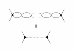
Figure 4: Chain of pair creation and annihilation of virtual massless fermion-antifermion pairs

The Higgs-like particle found in 2012 is now experimentally examined, and its properties are still hotly debated [27] [28]. Even in this simple $L_{0}(x)$ which acts on the physical vacuum $|\widetilde{0}\rangle$, the Higgs-like excitation naturally appears as a dynamical consequence. Whenever the massless fermions couple to gauge bosons in the condensed field-energy $\widehat{\beta}$ in Eq.(10), it is accompanied by another dynamical process. The annihilation of fermion-antifermion pair at $x$ in $\widehat{g}^{2}\bar{\varphi}(x)\widehat{\beta}\varphi(x)$ causes a local excitation $\beta(x)$ of gauge bosons in $\widehat{\beta}$. This excitation $\beta(x)$ annihilate to other massless fermion-antifermion pair at $x^{\prime}$. Hence, it propagates in space through a chain of creations and annihilations of massless fermion-antifermion pairs as illustrated in Figure 6. Because this mode causes a deviation from the lowest-energy state, it can be called Higgs-like excitation mode $H_{\beta}(x)$. Because this excitation has no special direction in space, it can be regarded as a scalar field. With $m_{f}=\widehat{g}^{2}\langle\widehat{\beta}\rangle$, the dynamical form of Eq.(10) is given by

$$\frac{m_{f}}{\langle\widehat{\beta}\rangle}\bar{\varphi}(x)H_{\beta}(x)\varphi(x).$$ (25)

This is a non-minimal interaction, because the gauge transformation occurs within $H_{\beta}(x)$ (excitation from $\widehat{\beta}$ in Eq.(6)), and does not cause the phase rotation of $\varphi(x)$. Hence, $\gamma^{\mu}$ matrix is not there. The bubble diagrams in Figure 6 shows a series of the creation and annihilation of the fermion-antifermion pair

$$q^{2}J(q^{2})=\frac{m_{f}}{\langle\widehat{\beta}\rangle}\int_{0}^{\Lambda}\frac{d^{4}p}{(2\pi)^{4}}tr\left[\frac{i}{/{\!\!\!}{p}-m_{f}}\frac{i}{/{\!\!\!}{p}+/{\!\!\!}{q}-m_{f}}\right].$$ (26)

This $J(q^{2})$ has following features.

(1) $J(q^{2})$ has a similar form to the vacuum polarization in QED [21], but an important difference is that there are no $\gamma^{\mu}$ or $\gamma^{\nu}$ in the trace.

(2) $\Lambda$ in Eq.(26) is not a cutoff for regularizing the divergent integral, but rather an upper end of the energy-momentum of the excited massless fermion-antifermion pairs. Eq.(26) can be calculated as if $\Lambda$ is such a cutoff for regularization, but since the upper end $\Lambda$ is a dynamical variable, it is evaluated, not as $p_{E}^{2}$ in the Euclidian space, but as $p^{2}=(ip_{0})^{2}-\mbox{\boldmath$p$}^{2}=-p_{E}^{2}$ in the Minkowski space. Hence, after 4-momentum integration, the square of upper end appears as $-\Lambda^{2}$.

According to the ordinary rule, we obtain

$$J(q^{2}) = \frac{1}{4\pi^{2}}\frac{m_{f}}{\langle\widehat{\beta}\rangle}\int_{0}^{1}dx\left[x(x-1)+\frac{m_{f}^{2}}{q^{2}}\right]$$ (27)

$$\times \ln\left(\frac{x(1-x)\Lambda^{2}+m_{f}^{2}}{x(x-1)q^{2}+m_{f}^{2}}\right).$$

A peculiar feature of this $J(q^{2})$ is that $m_{f}^{2}/q^{2}$ appears in the integrand. With this $J(q^{2})$, the propagator of the Higgs-like excitation mode $H_{\beta}(x)$ is given by

$$\int\frac{d^{4}x}{(2\pi)^{4}}\langle\widetilde{0}|T[H_{\beta}(x)H_{\beta}(0)]|\widetilde{0}\rangle e^{iqx}=\frac{1}{q^{2}\left[1-J(q^{2})\right]}.$$ (28)

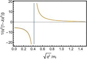
Figure 5: Propagator of the Higgs-like collective mode $1/(q^{2}[1-J(q^{2})])$ with $m_{f}/\langle\widehat{\beta}\rangle=0.64$ and $\Lambda/m_{f}=800$.

Figure 5 shows $1/(q^{2}[1-J(q^{2})])$ when $m_{f}/\langle\widehat{\beta}\rangle=0.64$ and $\Lambda/m_{f}=800$ are used as an example. A pole appears at $\sqrt{g^{2}}/m_{f}=0.42$ as if it is represented by $1/(q^{2}-m_{H}^{2})$ with the mass of Higgs-like boson $m_{H}=0.42m_{f}$. (The ratio $m_{H}/m_{f}$ depends on $\langle\widehat{\beta}\rangle$ and $\Lambda$.)

The nature of non-minimal interaction in Eq.(25) is the reason why the Higgs-like excitation mode $H_{\beta}(x)$ has a pole. The pole structure in Eq.(28) arises from $m_{f}^{2}/q^{2}$ in the integrand of Eq.(27), but this $m_{f}^{2}/q^{2}$ would not appear if $\gamma^{\mu}$ and $\gamma^{\nu}$ exist in the trace of Eq.(26).

In summary, the Higgs-like excitation is described by the following effective Lagrangian density

$$(\partial_{\mu}H_{\beta})^{2}-m_{H}^{2}H_{\beta}^{2}+\frac{m_{f}}{\langle\widehat{\beta}\rangle}\bar{\varphi}\varphi H_{\beta}.$$ (29)

The reason why the mass of the Higgs particle has been an unknown parameter in the electroweak model is that it is not a quantity infered from symmetry, but a result of the many-body phenomenon.

III.4.2 Mass and stability

The Higgs-like boson’s mass $m_{H}$ is strongly depends on the fermion’s mass $m_{f}$. But their relationship also depends on the parameter $\langle\widehat{\beta}\rangle$ and $\Lambda$. Figure 6 shows $m_{H}/m_{f}$, obtained by solving $J(m_{H}^{2})=1$, as a function of $m_{f}/\langle\widehat{\beta}\rangle$ and $\Lambda/m_{f}$. As these variables increase, it takes much energy $m_{H}$ to excite the Higgs-like mode.

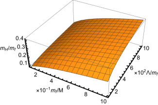
Figure 6: The rate of Higgs-like collective mode mass $m_{H}$ to fermion mass $m_{f}$ as a function of $m_{f}/\langle\widehat{\beta}\rangle$ and $\Lambda/m_{f}$. ($M$ denotes $\langle\widehat{\beta}\rangle$.)

This Higgs-like mode is unstable with respect to the decay into fermion-antifermion pairs at $q^{2}>(2m_{f})^{2}$. In Eq.(27), the logarithm function includes $x(x-1)q^{2}+m_{f}^{2}$ in the denominator, in which $x(x-1)$ is at most $-1/4$ at $x=1/2$. Hence, $x(x-1)+m_{f}^{2}/q^{2}$ becomes negative at $q^{2}>(2m_{f})^{2}$, which leads to an imaginary energy in Eq.(27). For any fixed $q^{2}$ at $q^{2}>(2m_{f})^{2}$, the $x$-value that can contribute to the imaginary energy in Eq.(27) satisfies $x(x-1)q^{2}+m_{f}^{2}<0$, which lies in a region between the points $x=\frac{1}{2}\pm\frac{1}{2}\delta$, where $\delta=\sqrt{1-4m_{f}^{2}/q^{2}}$. Using $Im[-X\pm i\epsilon]=\pm\pi$, and $y=x-\frac{1}{2}$, we obtain the imaginary part

$$- \frac{1}{4\pi^{2}}\frac{m_{f}}{\langle\widehat{\beta}\rangle}(\pm\pi)\int^{(1+\delta)/2}_{(1-\delta)/2}dx\left[x(x-1)+\frac{m_{f}^{2}}{q^{2}}\right]$$ (30)

$$= \pm\frac{1}{4\pi}\frac{m_{f}}{\langle\widehat{\beta}\rangle}\int^{\delta/2}_{-\delta/2}dy\left[(y^{2}-\frac{1}{4})+\frac{m_{f}^{2}}{q^{2}}\right].$$

Finally, we obtain the propagator of $H_{\beta}(x)$ at $q^{2}>(2m_{f})^{2}$ as follows

$$\int \frac{d^{4}x}{(2\pi)^{4}}\langle\widetilde{0}|TH_{\beta}(x)H_{\beta}(0)|\widetilde{0}\rangle e^{iqx}$$ (31)

$$= \frac{1}{q^{2}-m_{H}^{2}\pm i\displaystyle{\frac{1}{24\pi}\frac{m_{f}}{\langle\widehat{\beta}\rangle}\sqrt{1-\frac{4m_{f}^{2}}{q^{2}}}(q^{2}-4m_{f}^{2})}}.$$

in which $m_{H}^{2}$ is used for the real part of the logarithm function in Eq.(27). The imaginary part of the self energy increases with increasing $q^{2}$, and finally the excitation mode becomes unstable. For the electroweak interaction, however, we know $m_{H}=$125 GeV $<2m_{t}=$346 GeV. Since $m_{H}<2m_{f}$, the structure of the pole-mass around $q^{2}=m_{H}^{2}$ is not affected by the onset of damping at $q^{2}>(2m_{f})^{2}$.

IV Interim summary

The total Lagrangian density $L(x)$ is as follows. After rewriting $\varphi$ and $\bar{\varphi}$ with $\psi$ and $\bar{\psi}$, we obtain

$$L(x)= - \frac{1}{4}F^{\mu\nu}F_{\mu\nu}+m_{B}^{2}B^{\mu}B_{\mu}$$ (32)

$$+ \bar{\psi}(i\partial_{\mu}+gB_{\mu})\gamma^{\mu}\psi-m_{f}\bar{\psi}\psi$$

$$+ (\partial_{\mu}G)^{2}+m_{B}B_{\mu}\partial^{\mu}G+\frac{g}{m_{B}}\bar{\psi}\gamma^{\mu}\psi\partial_{\mu}G$$

$$+ (\partial_{\mu}H_{\beta})^{2}-m_{H}^{2}H_{\beta}^{2}+\frac{m_{f}}{\langle\widehat{\beta}\rangle}\bar{\psi}\psi H_{\beta}.$$

Compared to the Higgs model, this $L(x)$ has the following features.

(1) The Higgs potential is an economical phenomenology that explains much with a small number of parameters. This is because it plays a double role: the role of causing symmetry breaking in vacuum and that of predicting the Higgs particle’s mass. Furthermore, it stabilizes the broken-symmetry vacuum, and it further represents the interaction between the Higgs particle. However, that has made it difficult to imagine the physical processes behind it. In contrast, such a double role is dissolved in this $L(x)$. The broken-symmetry vacuum is derived from the kinematical requirement, and the Higgs particle’s mass is the result of the many-body phenomenon. Each role of the Higgs potential is played by each physical process.

(2) In the Higgs model, fermion’s mass is completely free parameter. In this $L(x)$, fermion’s mass and fermion’s coupling to Higgs-like excitation are not separated. Equation.(11) represents a $t$-channel process mediated by $\widehat{\beta}$, and Eq.(25) represents a $s$-channel process of the excitation of $\widehat{\beta}$.

(3) One of important predictions of the Higgs model is that the strength of the Higgs’s coupling to fermions is proportional to the fermion’s mass. This is explained by the $(m_{f}/\langle\widehat{\beta}\rangle)\bar{\psi}\psi H_{\beta}$ in this $L(x)$. Unlike the Yukawa coupling, however, the $(m_{f}/\langle\widehat{\beta}\rangle)\bar{\psi}\psi H_{\beta}$ in this $L(x)$ does not lead to the coupling of the Goldstone mode $G$ to the fermion. Rather, such a coupling $(g/m_{B})\bar{\psi}\gamma^{\mu}\psi\partial_{\mu}G$ in $L(x)$ arises from the structure of the physical vacuum.

(4) This $L(x)$ does not include $-4\lambda v_{h}h_{1}^{3}-\lambda h_{1}^{4}$ in the Higgs potential. Hence, the quadratic divergence does not occur in the perturbation calculation. The divergence we must renormalize is only logarithmic one, and there is no problem of fine-tuning.

(5) According to the lattice model, in which gauge invariance is strictly preserved at each stage of argument, the VEV of the gauge-dependent quantity vanishes, if it is calculated without gauge fixing, such as $\langle h(x)\rangle=0$ for $h(x)\rightarrow h(x)\exp(i\theta(x))$ under $A_{\mu}(x)\rightarrow A_{\mu}(x)-ig^{-1}\partial_{\mu}\theta(x)$ (Elitzur-De Angelis-De Falco-Guerra theorem) [22][23]. This is because the local character of gauge symmetry effectively breaks coupling between degrees of freedom localized in different space-time regions. If the Higgs particle is an elementary particle, the gauge-fixing dependence of its VEV does not match its fundamental nature. Instead of the single condensate $v_{h}=\langle h(x)\rangle$, the present physical vacuum is characterized by $\langle\widetilde{0}|\int j_{\mu}(Y)j^{\mu}(0)d^{4}Y|\widetilde{0}\rangle$ and $\langle\widetilde{0}|\int T_{c}^{00}(x)d^{3}x|\widetilde{0}\rangle=\langle\widehat{\beta}\rangle$. The former determines the gauge-boson’s mass $m_{B}$ in the first-order process of $g$. The latter determines the fermion’s mass $m_{f}$ in the second-order process of $g$. Because these two condensates in the form of integrals are gauge invariant, there is no need to worry about the vanishing of their VEV as in the VEV of gauge-dependent quantities.

V Effective coupling of the Higgs-like mode

For the electroweak interaction, the Glashaw-Weinberg-Salam (GWS) model using the Higgs model is a simple and successful model that does not contradict almost all experimental results to date [24][25][26]. So far, the Higgs coupling to the fermions, especially those of the third generation, have been well parameterized using the Yukawa coupling of fermions to the $h$. However, for more precise measurements, there is a possibility of deviation from such a simple parameterization. In the Higgs model, $\lambda|v_{h}+h|^{4}$ in the Higgs potential predicts the triple and quartic self-couplings of the Higgs particle $h_{1}$. They may correspond to more complex many-body effects than that in Figure 6, which are well known as collective excitations in the non-relativistic physics. The above $L(x)$ predicts some different results from those by the Higgs model. The next research subject is to extend it to the electroweak interaction.

Recently the decay of the Higgs-like particle to two gauge bosons $W^{+}$ and $W^{-}$ are observed [27][28]. Unlike $|(i\partial_{\mu}+gB_{\mu})(v_{h}+h)|^{2}$ in the Higgs model, there is no direct coupling of $H_{\beta}$ to $B_{\mu}$ in $L(x)$. Rather, the effective coupling of $H_{\beta}$ to $B_{\mu}$ appears first in the perturbation calculation through $(m_{f}/\langle\widehat{\beta}\rangle)\bar{\psi}\psi H_{\beta}$ and $g\bar{\psi}B_{\mu}\gamma^{\mu}\psi$ comes from one-loop processes illustrated in Figure 7. As a warmup example, we derive such an effective coupling in the case of $U(1)$ gauge field, and use it in the calculation of the cross section in Section.7. The result in Section.6 and 7 is obtained using the computing algorithm Package-X [29]. The future precise measurement of the electroweak interaction will determine whether the deviation from the simple Higgs model exists or not.

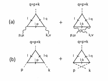
Figure 7: The effective coupling induced by the one-loop diagram (a) $\Gamma^{\mu\nu}_{BBH}(q,p,k,m_{B},m_{f})$ in Eq.(37), and (b) $F_{H}(q^{2},p^{2},k^{2},m_{f})$ in Eq.(46). Wavy and dotted lines represent $B_{\mu}$ and $H_{\beta}$, respectively.

V.1 Coupling to massive gauge bosons

The effective coupling term responsible for the $H_{\beta}$ decay into gauge bosons in Figure 7(a) is composed of $-(m_{f}/\langle\widehat{\beta}\rangle)\bar{\psi}\psi H_{\beta}$ and $\bar{\psi}gB_{\mu}\gamma^{\mu}\psi$ in Eq.(32). In coordinate space, such a coupling takes a form

$$g^{2}\frac{m_{f}}{\langle\widehat{\beta}\rangle}\times B^{\mu}(x_{1})B^{\nu}(x_{2})H_{\beta}(x_{3})\times\langle\widetilde{0}|$$

$$T\left[\int j_{\mu}(x_{1})d^{4}x_{1}\int j_{\nu}(x_{2})d^{4}x_{2}\int\bar{\varphi}(x_{3})\varphi(x_{3})d^{4}x_{3}\right]|\widetilde{0}\rangle.$$

(A) When this coupling is viewed from a distant point in space-time, it looks like a local phenomenon at $X=(x_{1}+x_{2}+x_{3})/3$ as

$$g^{2}\frac{m_{f}}{\langle\widehat{\beta}\rangle}\int B^{\mu}(X)B^{\nu}(X)H_{\beta}(X)d^{4}X$$

$$\times\langle\widetilde{0}|T\left[\int j_{\mu}(x_{1})\int j_{\nu}(x_{2})\int t(x_{3})d^{3}x_{1}d^{3}x_{1}d^{3}x_{3}\right]|\widetilde{0}\rangle,$$

where $t(x)=\bar{\varphi}(x)/{\!\!\!}{\partial}\varphi(x)$. The coefficient of $B^{\mu}B^{\nu}H_{\beta}$ is a three-point correlation function with a dimension of mass. Since the physical vacuum $|\widetilde{0}\rangle$ is filled with massless fermion-antifermion pairs, the coefficient of $g_{\mu\nu}B^{\mu}B^{\nu}H_{\beta}$ in Eq.(LABEL:eq:362) has a finite value $V_{h}$

$$V_{h}=\langle\widetilde{0}|T\left[\int j_{\mu}(x_{1})\int j^{\mu}(x_{2})\int t(x_{3})d^{3}x_{1}d^{3}x_{1}d^{3}x_{3}\right]|\widetilde{0}\rangle,$$ (35)

because of $\prod_{p,s}\sin\theta_{\mbox{\boldmath$p$}}e^{i\alpha(x)}b^{s\dagger}(-\mbox{\boldmath$p$})a^{s\dagger}(\mbox{\boldmath$p$})|0_{r}\rangle$ in $|\widetilde{0}\rangle$. This $V_{h}$ plays the role of $v_{h}$ in Eq.(8).

(B) When this coupling is viewed in high resolution, anomalous momentum-dependent coupling is observed. We consider an amplitude ${\cal M}[H_{\beta}(p+k)\rightarrow B_{\mu}(p)B_{\nu}(k)]$ in Figure 7(a)

$$g^{2}i{\cal M}[H_{\beta}(p+k)\rightarrow B_{\mu}(p)B_{\nu}(k)]$$ (36)

$$\propto(-ig)^{2}(-i\frac{m_{f}}{\langle\widehat{\beta}\rangle})$$

$$\quad\times\int\frac{d^{4}l}{(2\pi)^{4}}tr\left[\gamma^{\mu}\frac{i}{/{\!\!\!}{l}-/{\!\!\!}{p}-m_{f}}\gamma^{\nu}\frac{i}{/{\!\!\!}{l}-/{\!\!\!}{q}-m_{f}}\frac{i}{/{\!\!\!}{l}-m_{f}}\right]$$

$$\quad+(p\leftrightarrow k,\mu\leftrightarrow\nu).$$

Following the standard procedure, the analytic result is obtained as follows. The general form of the interaction between $B_{\mu}$ and $H_{\beta}$

$$g^{2} (\frac{m_{f}}{\langle\widehat{\beta}\rangle})\left[V_{h}g^{\mu\nu}+m_{f}\Gamma^{\mu\nu}_{BBH}(q,p,k,m_{B},m_{f})\right]$$ (37)

$$\times B_{\mu}(p)B_{\nu}(k)H_{\beta}(p+k),$$

has the following anomalous momentum-dependence

$$\Gamma^{\mu\nu}_{BBH}(q,p,k,m_{B},m_{f})$$ (38)

$$=F_{1}(q^{2},p^{2},k^{2},m_{f})g^{\mu\nu}$$

$$+F_{2}(q^{2},p^{2},k^{2},m_{f})\frac{p^{\nu}k^{\mu}+p^{\mu}k^{\nu}}{m_{B}^{2}}$$

$$+F_{3}(q^{2},p^{2},k^{2},m_{f})\frac{p^{\nu}p^{\mu}+k^{\mu}k^{\nu}}{m_{B}^{2}}.$$

In these $F_{i}$, the divergences coming from the triangle-loop integral are cancelled to each other in Eq.(36).

(a) We obtain the leading anomalous couplings $F_{1}(q^{2},p^{2},k^{2},m_{f})$ in Eq.(38) [30]

$$F_{1}(q^{2},p^{2},k^{2},m_{f})=$$ (39)

$$\frac{8}{(4\pi)^{2}}\left[1+\frac{(p^{2}+k^{2})q^{2}-8p^{2}k^{2}}{(q^{2}-4p^{2})(q^{2}-4k^{2})}f\left(\frac{q}{2m_{f}}\right)\right]$$

$$-\frac{8}{(4\pi)^{2}}\left[\frac{p^{2}}{q^{2}-4p^{2}}f\left(\frac{p}{2m_{f}}\right)+(p\leftrightarrow k)\right]$$

$$-\frac{2}{(4\pi)^{2}}\frac{q^{4}-(6p^{2}+4m_{f}^{2})q^{2}+4p^{4}+16p^{2}m_{f}^{2}}{q^{2}-4p^{2}}$$

$$\quad\times C_{0}(p^{2},p^{2},q^{2},m_{f}^{2},m_{f}^{2},m_{f}^{2})$$

$$-(p\leftrightarrow k),$$

where

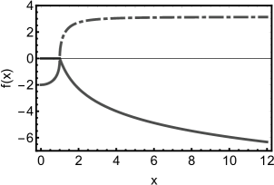
Figure 8: Schematic view of $f(x)$. $Ref(x)$ and $Imf(x)$ are represented by a solid, and a one-point-dotted curve, respectively.

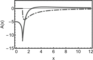
Figure 9: Schematic view of $A(x)$. $ReA(x)$ and $ImA(x)$ are represented by a solid, and a one-point-dotted curve, respectively.

(1) The function $f(x)$

$$f(x)=\sqrt{1-\frac{1}{x^{2}}}\ln\left[1-2x^{2}+2x^{2}\sqrt{1-\frac{1}{x^{2}}}\right],$$ (40)

is illustrated in Figure.8.

(2) $C_{0}(p^{2},p^{2},q^{2},m_{f}^{2},m_{f}^{2},m_{f}^{2})$ is the scalar $C_{0}$ function in the Passarino-Veltman integrals [31][32],

$$C_{0}(p^{2},p^{2},q^{2},m_{f}^{2},m_{f}^{2},m_{f}^{2})$$

$$=\frac{2}{q^{2}}A(\frac{q}{2m_{f}})+\left(\frac{1}{m_{f}^{2}q^{2}}+\frac{1}{q^{4}}A(\frac{q}{2m_{f}})\right)p^{2}+\cdots,$$

where

$$A(x)=-\arcsin^{2}x$$ (42)

for for $x<1$, and

$$A(x)=\frac{1}{4}\left(\ln\displaystyle{\left[1-2x^{2}+2x^{2}\sqrt{1-\frac{1}{x^{2}}}\right]}-i\pi\right)^{2},$$ (43)

for $x>1$, which is illustrated in Figure.9. Since $f(x)\rightarrow-2$ and $\arcsin x\rightarrow x$ at $x\rightarrow 0$, $F_{1}(0,0,0,m_{f})=0$ is obtained in Eq.(39).

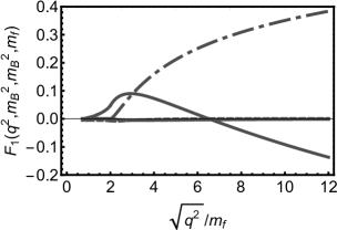
Figure 10: The overall $q^{2}$-dependence of the anomalous effective coupling $F_{1}(q^{2},m_{B}^{2},m_{B}^{2},m_{f})$; the real part $ReF_{1}$ (solid curve), and its imaginary part $ImF_{1}$ (one-point-dotted curve). The mass of the gauge boson $B_{\mu}$ is $m_{B}=80$ GeV. The mass $m_{H}$ of $H_{\beta}$ and the mass $m_{f}$ of the fermion in the triangle loop are assumed as $m_{H}=123$ GeV and $m_{f}=160$ GeV, respectively. The condition of $q^{2}=m_{H}^{2}$ corresponds to $\sqrt{q^{2}}/m_{f}=0.76$, from which $F_{1}(q^{2})$ begins to exist. The solid curve at $\sqrt{q^{2}}/m_{f}<2$ is magnified in Figure.11.

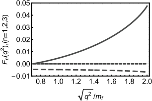
Figure 11: Three types of the real part of anomalous effective coupling at $\sqrt{q^{2}}<2m_{f}$, $F_{1}(q^{2},m_{B}^{2},m_{B}^{2},m_{f})$ (solid curve), $F_{2}(q^{2},m_{B}^{2},m_{B}^{2},m_{f})$ (dotted curve), and $F_{3}(q^{2},m_{B}^{2},m_{B}^{2},m_{f})$ (short dotted curve), under the same condition as Figure 10.

(b) For the decay $H_{\beta}(p+k)\rightarrow B_{\mu}(p)B_{\nu}(k)$ illustrated in Figure 7(a), we numerically calculate the anomalous effective coupling at $p^{2}=k^{2}=m_{B}^{2}$. Figure 10 shows the overall $q^{2}$-dependence of $F_{1}(q^{2},m_{B}^{2},m_{B}^{2},m_{f})$: its real part $ReF_{1}$ (solid curve), and its imaginary part $ImF_{1}$ (one-point-dotted curve), in which $m_{B}=80$ GeV, $m_{H}=123$ GeV, and $m_{f}=160$ GeV are used. The real part $ReF_{1}(q^{2},m_{B}^{2},m_{B}^{2},m_{f})$ increases with increasing $\sqrt{q^{2}}$ to $2m_{f}$, and decreases at $\sqrt{q^{2}}>2m_{f}$, then changing its sign. The amplitude of imaginary part $ImF_{1}(q^{2},m_{B}^{2},m_{B}^{2},m_{f})$ remains zero at $\sqrt{q^{2}}<2m_{f}$, but gradually increases at $\sqrt{q^{2}}>2m_{f}$.

(c) In the present model, other effective anomalous couplings $F_{2}(q^{2},p^{2},k^{2},m_{f})$ and $F_{3}(q^{2},p^{2},k^{2},m_{f})$ inevitably appears. (See Appendix). Figure 11 shows $ReF_{1}$, $ReF_{2}$ and $ReF_{3}$ at $\sqrt{q^{2}}<2m_{f}$, in the case of same $m_{f}$, $m_{B}$, $m_{H}$ as in Figure 10. $ReF_{2}$ and $ReF_{3}$ are much smaller than $ReF_{1}$. The imaginary parts $ImF_{1}$, $ImF_{2}$ and $ImF_{3}$ are zero in $\sqrt{q^{2}}<2m_{f}$.

V.2 Self coupling

The effective self-coupling of the Higgs-like mode is created by the one-loop process illustrated in Figure 7(b). In coordinate space, this coupling is expressed by another three-point correlation $W_{h}$

$$W_{h}=\langle\widetilde{0}|T\left[\int\widetilde{t}(x_{1})\int\widetilde{t}(x_{2})\int t(x_{3})d^{3}x_{1}d^{3}x_{1}d^{3}x_{3}\right]|\widetilde{0}\rangle,$$ (44)

where $\widetilde{t}(x)=\bar{\varphi}(x)\varphi(x)$. The anomalous momentum-dependent self-coupling is obtained by the following amplitude

$$i{\cal M}[H_{\beta}(p+k)\rightarrow H_{\beta}(p)H_{\beta}(k)]$$ (45)

$$\propto(-i\frac{m_{f}}{\langle\widehat{\beta}\rangle})^{3}\int\frac{d^{4}l}{(2\pi)^{4}}tr\left[\frac{i}{/{\!\!\!}{l}-/{\!\!\!}{p}-m_{f}}\frac{i}{/{\!\!\!}{l}-/{\!\!\!}{q}-m_{f}}\frac{i}{/{\!\!\!}{l}-m_{f}}\right]$$

$$+(p\leftrightarrow k).$$

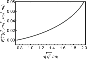
Figure 12: The renormalized anomalous effective self-coupling $F^{ren}_{H}(q^{2},m_{H}^{2},m_{H}^{2},m_{f})$ of Higgs-like mode, for the decay of off-shell such a mode into two on-shell such modes, in the case of same $m_{H}$ and $m_{f}$ as in Figure 10. The condition of $q^{2}=m_{H}^{2}$ corresponds to $\sqrt{q^{2}}/m_{f}=0.76$.

Hence, the effective self-coupling of the Higgs-like mode has a form such as

$$(\frac{m_{f}}{\langle\widehat{\beta}\rangle})^{3}[W_{h}+m_{f}F_{H}(q^{2},p^{2},k^{2},m_{f})]H_{\beta}(p)H_{\beta}(k)H_{\beta}(p+k),$$ (46)

which corresponds to $\lambda v_{h}$ in Eq.(8). This $(m_{f}/\langle\widehat{\beta}\rangle)^{3}W_{h}$ no longer plays the role of stabilizing the symmetry-broken vacuum as in the Higgs potential in $L_{h}(x)$.

Following the standard procedure, we calculate the anomalous self-coupling, and find that the divergence $1/\epsilon$ coming from the triangular-loop integrals does not cancel each other in Eq.(45). We set a condition that $F_{H}(q^{2},p^{2},k^{2},m_{f})$ is zero at the on-shell level, and has a finite value only at the off-shell level $q^{2}>m_{H}^{2}$. Hence, $F_{H}(q^{2},p^{2},k^{2},m_{f})$ must vanish at $q^{2}=m_{H}^{2}$. (For the divergence that is independent of momentum, it is to be renormalized to $W_{h}$.) We define the renormalized one as $F^{ren}_{H}(q^{2},p^{2},k^{2},m_{f})=F_{H}(q^{2},p^{2},k^{2},m_{f})-F_{H}(m_{H}^{2},p^{2},k^{2},m_{f})$, and obtain

$$F^{ren}_{H}(q^{2},p^{2},k^{2},m_{f})=\frac{8}{(4\pi)^{2}}\left[f\left(\frac{q}{2m_{f}}\right)-f\left(\frac{m_{H}}{2m_{f}}\right)\right]$$ (47)

$$+\frac{2}{(4\pi)^{2}}(8m_{f}^{2}-2p^{2}-q^{2})C_{0}(p^{2},p^{2},q^{2},m_{f}^{2},m_{f}^{2},m_{f}^{2})$$

$$-\frac{2}{(4\pi)^{2}}(8m_{f}^{2}-2p^{2}-m_{H}^{2})C_{0}(p^{2},p^{2},m_{H}^{2},m_{f}^{2},m_{f}^{2},m_{f}^{2})$$

$$+(p\leftrightarrow k).$$

For the decay $H_{\beta}(p+k)\rightarrow H_{\beta}(p)H_{\beta}(k)$ in Figure 7(b), we numerically calculate $F^{ren}_{H}(q^{2},m_{H}^{2},m_{H}^{2},m_{f})$. Figure 12 shows the result under the same $m_{H}$ and $m_{f}$ as in Figure 10. This effective coupling gradually increases from zero with increasing $\sqrt{q^{2}}$ to $2m_{f}$. The overall $q^{2}$-dependence of $F^{ren}_{H}(q^{2},m_{H}^{2},m_{H}^{2},m_{f})$ is quite similar to $F_{1}(q^{2},m_{B}^{2},m_{B}^{2},m_{f})$, except for its absolute value.

VI Pair annihilation of fermion and antifermion to gauge boson pair

As an example of the reaction including the production and decay of the Higgs-like mode, we consider a $s$-channel process: fermion $\psi(p_{1})$ + antifermion $\bar{\psi}(k_{1})$ $\rightarrow H_{\beta}(q)$ $\rightarrow B_{\mu}(p)$ +$B_{\nu}(k)$ illustrated in Figure.13. This reaction occurs together with the background reactions, such as the tree process through the $t$- and $u$-channel exchanges of fermion. The cross section of such a tree process is a slowly and monotonously decreasing function of the center-of-mass energy $E_{cm}$. In the total cross section, the effective coupling of the Higgs-like mode will appear above this almost constant background cross section. In view of Figure 10 and 11, we use only $F_{1}(q^{2},m_{B}^{2},m_{B}^{2},m_{f})$ as the first approximation of the total effective coupling. We obtain the amplitude of the process in Figure.13

$$i{\cal M}=\frac{m_{f}}{\langle\widehat{\beta}\rangle}\bar{V}(k_{1})U(p_{1})g^{2}\frac{m_{f}}{\langle\widehat{\beta}\rangle}$$

$$\times\frac{\displaystyle{\left[V_{h}+m_{f}[ReF_{1}(q^{2})+iImF_{1}(q^{2})]\right]}}{q^{2}-m_{H}^{2}\pm i\displaystyle{\frac{1}{24\pi}\frac{m_{f}}{\langle\widehat{\beta}\rangle}\sqrt{1-\frac{4m_{f}^{2}}{q^{2}}}(q^{2}-4m_{f}^{2})}}\epsilon^{\mu}(p)\epsilon_{\mu}(k),$$

where $\epsilon^{\mu}(p)$ is one of polarization vectors of the massive gauge boson, satisfying $\epsilon^{\mu}(p)\epsilon_{\mu}(p)=-1$ for longitudinal and transverse polarizations.

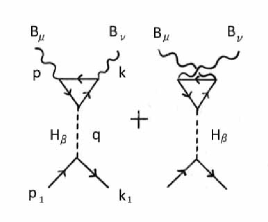
Figure 13: Fermion-antifermion pair annihilation through the intermediate Higgs-like mode to gauge boson pair.

Since the incident fermion and antifermion are lighter than the particles in the triangle loop, the former are assumed to be massless. Using $\sum_{s}U(p_{1})\bar{U}(p_{1})=/{\!\!\!}{p_{1}}$ and $\sum_{s}V(k_{1})\bar{V}(k_{1})=/{\!\!\!}{k_{1}}$, we obtain the squared amplitude

$$\frac{1}{4}\sum_{s,s^{\prime}}|{\cal M}|^{2}=g^{4}\left(\frac{m_{f}}{\langle\widehat{\beta}\rangle}\right)^{4}12(p_{1}\cdot k_{1})$$

$$\times\frac{\displaystyle{[V_{h}+m_{f}ReF_{1}(q)]^{2}+m_{f}^{2}[ImF_{1}(q)]^{2}}}{(q^{2}-m_{H}^{2})^{2}+\displaystyle{\left(\frac{1}{24\pi}\frac{m_{f}}{\langle\widehat{\beta}\rangle}\right)^{2}\left(1-\frac{4m_{f}^{2}}{q^{2}}\right)(q^{2}-4m_{f}^{2})^{2}}}.$$

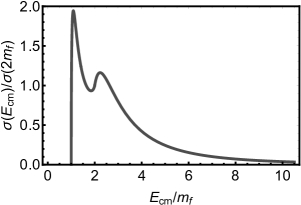
Figure 14: The rate of total cross section $\sigma(E_{cm})$ to $\sigma(2m_{f})$ in the fermion-antifermion annihilation to gauge boson pair through the intermediate Higgs-like collective mode, in the case of $m_{B}=80$ GeV, $m_{f}=160$ GeV, $m_{H}=123$ GeV and $V_{h}/m_{f}=0.02$.

In the center-of-mass frame where $p_{1}=(E_{cm}/2,\mbox{\boldmath$p$}_{1})$ and $k_{1}=(E_{cm}/2,-\mbox{\boldmath$p$}_{1})$, we can use $q^{2}=(p_{1}+k_{1})^{2}=E_{cm}^{2}$ and $p_{1}\cdot k_{1}=E_{cm}^{2}/2$. The total cross section $\sigma(E_{cm})$ is given by

$$\sigma(E_{cm})=\frac{\pi}{E_{cm}^{2}}\sqrt{1-\frac{4m_{B}^{2}}{E_{cm}^{2}}}\sum_{s,s^{\prime}}|{\cal M}|^{2}.$$ (50)

Figure 14 shows the rate of total cross section $\sigma(E_{cm})$ to $\sigma(2m_{f})$ in the case of $V_{h}/m_{f}=0.02$, and same $m_{f}$, $m_{B}$, $m_{H}$ as in Figure 10. The steep rise of $\sigma$ occurs at $E_{cm}=2m_{B}$. In contrast to the Higgs model, $\sigma$ gradually increases below $E_{cm}=2.3m_{f}$, and later decreases at $E_{cm}>2.3m_{f}$, which are peculiar feature of the Higgs-like excitation mode. The smaller the rate $V_{h}/m_{f}$ is in Eq.(LABEL:eq:615), this gradual increase and decrease of $\sigma(E_{cm})$ is is more clearly observed around $E_{cm}=2.3m_{f}$. (If $m_{H}>2m_{B}$, a sharp resonance peak representing a pole at $q^{2}=m_{H}^{2}$ also appears.) This $E_{cm}$-dependence mainly comes from $ReF_{1}$ and $ImF_{1}$. It is not affected by the damping of the Higgs-like mode $H_{\beta}$, because the effect of damping is weakened by the small factor $(1/24\pi)^{2}$ in Eq.(LABEL:eq:615). The gradual increase and decrease of the cross section around $E_{cm}=2.3m_{f}$ is a key feature for the experimental confirmation of the physical vacuum, which is absent in $L_{h}(x)$.

VII Renormalizability

In the Higgs model, symmetry breaking is caused simply by changing the sign of the coefficient $\mu^{2}$ in the Higgs potential $-\mu^{2}|v_{h}+h|^{2}+\lambda|v_{h}+h|^{4}$. Renormalizability of the Higgs model is systematically proved using the generating functional with this Higgs potential [33]. (1) In the symmetric vacuum, this generating functional is expanded in powers of the Higgs field $h(x)$. In the symmetry-broken vacuum, it is expanded in powers of $h(x)-v_{h}$. The algebraic relationship between these two types of expansion can be obtained, which assures that the renormalizability of the theory in the symmetric vacuum can be transferred to that in the symmetry-broken one. (2) When the Bogoliubov-Parasuik-Hepp-Zimmermann (BPHZ) method is applied to the Ward-Takahashi identities derived from this generating functional, renormalizability is systematically proved without reference to the symmetric model [34].

In the present model using $L_{3}(x)$ in Eq.(32), however, the Higgs potential is not assumed. Hence, we can not immediately apply this systematic method. Rather, we go back to the inductive proof of renormalizability originated by Dyson in QED [35]. Let us consider the following Green’s functions: $S(p)$ for the massive fermion $\psi$,

$$[S(p)]^{-1}=-\gamma\cdot p+m_{f}-\Sigma^{*}(p),$$ (51)

$D(p^{2})$ for the massive gauge boson $B_{\mu}$ in Eq.(22),

$$[D(p^{2})]^{-1}=-p^{2}+m_{B}^{2}-\Pi^{*}(p^{2}),$$ (52)

and $G(p^{2})$ for the Higgs-like mode $H_{\beta}$

$$[G(p^{2})]^{-1}=-p^{2}+m_{H}^{2}-\Pi_{H}^{*}(p^{2}).$$ (53)

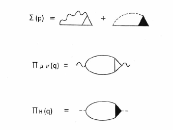
Figure 15: (a) Self energy $\Sigma(p)$ of the fermion $\psi$, (b) Vacuum polarization $\Pi_{\mu\nu}(q)$ of the gauge field $B_{\mu}$, (c) Vacuum polarization $\Pi_{H}(q)$ of the Higgs-like mode $H_{\beta}$. Wavy and dotted lines represent $B_{\mu}$ and $H_{\beta}$, respectively. A white triangle denotes a vertex $\Gamma_{\mu}$ between $B_{\mu}$ and $\psi$, and a black triangle denotes $\widehat{\Gamma}_{H}$ between $H_{\beta}$ and $\psi$.

The self energy $\Sigma^{*}(p)$ of fermions satisfies the following Dyson equations illustrated in Figure 15,

$$i\Sigma^{*}(p) = \frac{g^{2}}{(2\pi)^{4}}\int d^{4}k\gamma_{\nu}S(p-k)\Gamma_{\mu}(p-k,p)D^{\mu\nu}(k)$$ (54)

$$+ \frac{1}{(2\pi)^{4}}\left(\frac{m_{f}}{\langle\widehat{\beta}\rangle}\right)^{2}\int d^{4}kS(p-k)\widehat{\Gamma}_{H}(p-k,p)G(k)$$

$$\equiv i\Sigma_{1}(p)+i\Sigma_{2}(p)$$

where the vertex $\Gamma_{\mu}$ illustrated by a white triangle is the vertex function between $B_{\mu}$ and $\psi$, and another vertex $\widehat{\Gamma}_{H}$ illusrated by a black triangle is the vertex function between $H_{\beta}$ and $\psi$. Correspondingly, the self energy $\Sigma(p)$ of fermion is composed of $\Sigma_{1}(p)$ due to the coupling to $B_{\mu}$, and $\Sigma_{2}(p)$ due to the coupling to $H_{\beta}$ [36].

Similarly, the vacuum polarization $\Pi_{\mu\nu}^{*}(p^{2})$ of the massive gauge boson satisfies

$$i\Pi_{\mu\nu}^{*}(p^{2})=\frac{g^{2}}{(2\pi)^{4}}\int d^{4}ktr[S(p+k)\gamma_{\mu}S(k)\Gamma_{\nu}(k,p+k)],$$ (55)

and the vacuum polarization $\Pi_{H}^{*}(p^{2})$ of the Higgs-like mode satisfies

$$i\Pi_{H}^{*}(p^{2})=\frac{g^{2}}{(2\pi)^{4}}\int d^{4}ktr[S(p+k)S(k)\widehat{\Gamma}_{H}(k,p+k)].$$ (56)

VII.1 The vertex $\Gamma_{\mu}(p,p^{\prime})$ between $B_{\mu}$ and $\psi$

For the vertex $\Gamma_{\mu}(p,p^{\prime})=\gamma_{\mu}+\Lambda_{\mu}^{*}(p,p^{\prime})$ between $B_{\mu}$ and $\psi$ in Eq.(54), its proper vertex $\Lambda_{\mu}^{*}(p,p^{\prime})$ satisfies the following Dyson equation as illustrated in Figure 16(a)

$$\Lambda_{\mu}^{*}(p,p^{\prime})$$ (57)

$$=\frac{g^{2}}{(2\pi)^{4}}\int d^{4}k\Gamma_{\nu}(p+k,k)S(p+k)D^{\nu\rho}(k)$$

$$\quad\times\Gamma_{\rho}(k,k+p^{\prime})S(-p^{\prime}+k)\Gamma_{\mu}(p+k,-p^{\prime}+k)$$

$$+\frac{1}{(2\pi)^{4}}\left(\frac{m_{f}}{\langle\widehat{\beta}\rangle}\right)^{2}\int d^{4}k\widehat{\Gamma}_{H}(p+k,k)S(p+k)G(k)$$

$$\quad\times\widehat{\Gamma}_{H}(k,k+p^{\prime})S(-p^{\prime}+k)\Gamma_{\mu}(p+k,-p^{\prime}+k)$$

$$+\cdots.$$

Figure 16: (a) Proper vertex $\Lambda_{\mu}$ between the fermion $\psi$ and the gauge field $B_{\mu}$, (b) Proper vertex $\Lambda_{H}$ between the fermion $\psi$ and the Higgs-like mode $H_{\beta}$.

This $\Lambda_{\mu}^{*}(p,p^{\prime})$ is related to the fermion self-energy $\Sigma_{1}^{*}(p)$ (due to the coupling to $B_{\mu}$) as [37]

$$\frac{\partial}{\partial p_{\mu}}\Sigma_{1}^{*}(p)=\Lambda_{\mu}(p,p).$$ (58)

Similarly, if we consider a proper vertex $\Lambda_{H}(p,p^{\prime})$ for $\widehat{\Gamma}_{H}(p,p^{\prime})=1+\Lambda_{H}(p,p^{\prime})$ between $H_{\beta}$ and $\psi$ in Eq.(54), it satisfies the Dyson equation illustrated in Figure 16(b). The other fermion self-energy $\Sigma_{2}(p)$ (due to the coupling to $H_{\beta}$) is related to this $\Lambda_{H}$ as

$$\frac{\partial}{\partial p}\Sigma_{2}^{*}(p)=\Lambda_{H}(p,p).$$ (59)

With these $\Lambda_{\mu}(p,p)$ and $\Lambda_{H}(p,p)$, we obtain the Green function of fermions

$$[S(p)]^{-1}=-\gamma\cdot p+m_{f}-\int_{p_{0}}^{p}dk^{\mu}\Lambda_{\mu}(k,k)-\int_{p_{0}}^{p}dk\Lambda_{H}(k,k).$$ (60)

We will introduce the following renormalization-constants $Z_{i}$ ($i=1\sim 5$ )

$$S(p)=Z_{2}S^{ren}(p),$$ (61)

$$D_{\mu\nu}(p^{2})=Z_{3}D_{\mu\nu}^{ren}(p^{2}),$$ (62)

$$G(p^{2})=Z_{5}G^{ren}(p^{2}),$$ (63)

$$\Gamma_{\mu}(p,p^{\prime})=Z_{1}^{-1}\Gamma_{\mu}^{ren}(p,p^{\prime}),$$ (64)

$$\widehat{\Gamma}_{H}(p,p^{\prime})=Z_{4}^{-1}\widehat{\Gamma}_{H}^{ren}(p,p^{\prime}).$$ (65)

Let us estimate the divergence appearing successively in the perturbation expansion in Eq.(57).

(1) In the expansion of $\Lambda_{\mu}(p,p^{\prime})$, we focus on $\Lambda_{\mu}$ of the order of $g^{2j}$ obtained by $j$ times of iteration. These $\Lambda_{\mu}$ contain $2j$ $S(p)$, $j$ $D(p^{2})$, and $2j$ $\Gamma_{\mu}(p,p^{\prime})$, in addition to the original $\Gamma_{\mu}$. When $S(p)$, $D(p^{2})$, $\Gamma_{\mu}$ and $\widehat{\Gamma}_{H}$ are replaced by their counterparts in Eqs.(61) $\sim$ (65), this $\Lambda_{\mu}(p,p^{\prime})$ is renormalized as

$$\Lambda_{\mu}(p,p^{\prime})=(Z_{1}^{-1}Z_{2}Z_{3}^{1/2})^{2j}Z_{1}^{-1}\Lambda_{\mu}^{ren}(p,p^{\prime}),$$ (66)

(2) Next, we focus on each $\Lambda_{\mu}$ of the order of $(m_{f}/\langle\widehat{\beta}\rangle)^{2j}$. In addition to the original $\Gamma_{\mu}$, they contain $2j$ $S(p)$, $j$ $G(p^{2})$, and $2j$ $\widehat{\Gamma}_{H}(p,p^{\prime})$. Hence, this $\Lambda_{\mu}(p,p^{\prime})$ is renormalized as

$$\Lambda_{\mu}(p,p^{\prime})=(Z_{4}^{-1}Z_{2}Z_{5}^{1/2})^{2j}Z_{1}^{-1}\Lambda_{\mu}^{ren}(p,p^{\prime}),$$ (67)

If $g$ is replaced by

$$g^{ren}=Z_{1}^{-1}Z_{2}Z_{3}^{1/2}g,$$ (68)

and $\langle\widehat{\beta}\rangle$ by

$$\langle\widehat{\beta}\rangle_{ren}^{-1}=Z_{4}^{-1}Z_{2}Z_{5}^{1/2}\langle\widehat{\beta}\rangle^{-1},$$ (69)

the total proper vertex is renormalized as

$$\Lambda_{\mu}(p,p^{\prime})=Z_{1}^{-1}\Lambda_{\mu}^{ren}(p,p^{\prime},g^{ren},\langle\widehat{\beta}\rangle_{ren}),$$ (70)

For the higher-order terms with various combination of $g^{2}$ and $(m_{f}/\langle\widehat{\beta}\rangle)^{2}$, similar renormalization is possible.

VII.2 The vertex $\widehat{\Gamma}_{H}(p,p^{\prime})$ between $H_{\beta}$ and $\psi$

For the vertex $\widehat{\Gamma}_{H}(p,p^{\prime})=1+\Lambda_{H}(p,p^{\prime})$ between $H_{\beta}$ and $\psi$ in Figure 16(b), the proper vertex $\Lambda_{H}(p,p^{\prime})$ has a similar structure to $\Lambda_{\mu}(p,p^{\prime})$ if $\Gamma_{\mu}$ for the external $B_{\mu}$ is replaced by $\widehat{\Gamma}_{H}$ for the external $H_{\beta}$. Hence, using Eqs.(68) and (69), $\Lambda_{H}(p,p^{\prime})$ is renormalized as

$$\Lambda_{H}(p,p^{\prime})=Z_{4}^{-1}\Lambda_{H}^{ren}(p,p^{\prime},g^{ren},\langle\widehat{\beta}\rangle_{ren}),$$ (71)

and $Z_{1}=Z_{4}$. Since Eqs.(58) and (59) also hold for the renormalized quantities, $Z_{2}=Z_{1}=Z_{4}$ is obtained. Using Eqs.(70) and Eq.(71) in (60), we obtain the total renormalized fermion self-energy $\Sigma^{ren}(p)=\Sigma^{*}_{1}(p)+\Sigma^{*}_{2}(p)$, and the renormalized $S^{ren}(p)$.

VII.3 The vacuum polarization $\Pi(p)$ of the massive gauge field $B_{\mu}$

For the vacuum polarization $\Pi^{*}(p)$ of $B_{\mu}$ in Eq.(52), the proper vertex $\Delta_{\mu}(p,p^{\prime})$ satisfying

$$\frac{\partial}{\partial p_{\mu}}\Pi^{*}(p)=\Delta_{\mu}(p,p),$$ (72)

is defined. This $\Delta_{\mu}(p,p)$ is useful, because the Green’s function $D(p^{2})$ of $B_{\mu}$ is expressed as

$$[D(p^{2})]^{-1}=-p^{2}+m_{B}^{2}-\int_{p^{\prime}_{0}}^{p}dk^{\mu}\Delta_{\mu}(k,k).$$ (73)

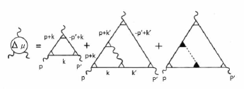
Figure 17: Proper vertex $\Delta_{\mu}$ between the gauge fields $B_{\mu}$.

This $\Delta_{\mu}(p,p^{\prime})$ satisfies the following Dyson equation illustrated in Figure 17

$$\Delta_{\mu}^{*}(p,p^{\prime})=\frac{g^{2}}{(2\pi)^{4}}\int d^{4}k\Gamma_{\nu}(p+k,k)S(p+k)S(k)$$ (74)

$$\mbox{ }\times\Gamma_{\nu}(k,k+p^{\prime})S(-p^{\prime}+k)\Gamma_{\mu}(p+k,-p^{\prime}+k)$$

$$+\frac{g^{4}}{(2\pi)^{8}}\int d^{4}kd^{4}k^{\prime}\Gamma_{\nu}(p+k,k)S(p+k)\Gamma_{\sigma}(p+k,p^{\prime}+k)$$

$$\mbox{ }\times S(p+k^{\prime})S(k)\Gamma_{\tau}(k,k^{\prime})D^{\sigma\tau}(k-k^{\prime})S(k^{\prime})$$

$$\mbox{ }\times\Gamma_{\nu}(k^{\prime},-p^{\prime}+k^{\prime})S(k^{\prime}-p^{\prime})\Gamma_{\mu}(p+k^{\prime},-p^{\prime}+k^{\prime})$$

$$+\frac{1}{(2\pi)^{8}}g^{2}\left(\frac{m_{f}}{\langle\widehat{\beta}\rangle}\right)^{2}\int d^{4}kd^{4}k^{\prime}\Gamma_{\nu}(p+k,k)S(p+k)$$

$$\mbox{ }\times\widehat{\Gamma}_{H}(p+k,p^{\prime}+k)S(p+k^{\prime})$$

$$\mbox{ }\times S(k)\widehat{\Gamma}_{H}(k,k^{\prime})G(k-k^{\prime})S(k^{\prime})\Gamma^{\nu}(k^{\prime},-p^{\prime}+k^{\prime})$$

$$\mbox{ }\times S(k^{\prime}-p^{\prime})\Gamma_{\mu}(p+k^{\prime},-p^{\prime}+k^{\prime})$$

$$+\cdots.$$

Only few terms are written in the above expansion, but it extends to the higher-order terms of $g^{2}$ and $(m_{f}/\langle\widehat{\beta}\rangle)^{2}$.

(1) Let us consider $\Delta_{\mu}$ of the order of $g^{2j}$ in the above expansion. They contain $(2j+1)$ $S(p)$, $(j-1)$ $D_{\mu\nu}(p^{2})$, and $(2j+1)$ $\Gamma_{\mu}(p,p^{\prime})$ [38]

$$\Delta_{\mu}(p,p^{\prime}) = Z_{2}^{2j+1}Z_{3}^{j-1}Z_{1}^{-(2j+1)}\Delta^{ren}_{\mu}(p,p^{\prime})$$

$$= Z_{2}^{2j+1}Z_{3}^{j-1}Z_{1}^{-2j}Z_{2}^{-1}\Delta^{ren}_{\mu}(p,p^{\prime})$$

$$= (Z_{1}^{-1}Z_{2}Z_{3}^{1/2})^{2j}Z_{3}^{-1}\Delta^{ren}_{\mu}(p,p^{\prime}).$$

Hence, if we replace $g$ by $g^{ren}$ defined in Eq.(68), each $\Delta_{\mu}$ with $g^{2j}$ is renormalized.

(2) Similarly, for $\Delta_{\mu}$ with the coefficient $g^{i}(m_{f}/\langle\widehat{\beta}\rangle)^{j}$, it contains $(i+j+1)$ $S(p)$, $(i/2-1)D_{\mu\nu}(p)$, $j/2$ $G(p^{2})$, $(i+1)$ $\Gamma_{\mu}(p,p^{\prime})$, and $j$ $\widehat{\Gamma}_{H}(p,p^{\prime})$ [39]

$$\Delta_{\mu}(p,p^{\prime}) = Z_{2}^{i+j+1}Z_{3}^{i/2-1}Z_{5}^{j/2}Z_{1}^{-(i+1)}Z_{4}^{-j}\Delta^{ren}_{\mu}(p,p^{\prime})$$

$$= (Z_{1}^{-1}Z_{2}Z_{3}^{1/2})^{i}(Z_{4}^{-1}Z_{2}Z_{5}^{1/2})^{j}Z_{3}^{-1}\Delta^{ren}_{\mu}(p,p^{\prime}).$$

Hence, if we replace $g$ by $g^{ren}$ in Eq.(68), and $\langle\widehat{\beta}\rangle$ by $\langle\widehat{\beta}\rangle_{ren}$ in Eq.(69), each $\Delta_{\mu}$ with $g^{i}(m_{f}/\langle\widehat{\beta}\rangle)^{j}$ is renormalized.

(3) As a result, the total proper vertex in Figure.17 is renormalized as

$$\Delta_{\mu}(p,p^{\prime})=Z_{3}^{-1}\Delta_{\mu}^{ren}(p,p^{\prime},g^{ren},\langle\widehat{\beta}\rangle_{ren}).$$ (77)

Using Eq.(77) in Eq.(73), we obtain the renormalized $D^{ren}(p^{2})$.

For the higher terms, similar renormalization is possible.

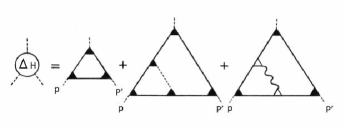
Figure 18: Proper vertex $\Delta_{H}$ between the Higgs-like modes $H_{\beta}$.

VII.4 The vacuum polarization $\Pi_{H}(p)$ of the Higgs-like mode $H_{\beta}$

For the vacuum polarization $\Pi_{H}(p)$ of the Higgs-like mode $H_{\beta}$ in Eq.(53), the proper vertex $\Delta_{H}(p,p^{\prime})$ satisfying

$$\frac{\partial}{\partial p}\Pi^{*}_{H}(p)=\Delta_{H}(p,p),$$ (78)

is defined. This $\Delta_{H}(p,p)$ is useful, because the Green’s function $G(p^{2})$ of the Higgs-like mode $H_{\beta}$ is expressed as

$$[G(p^{2})]^{-1}=-p^{2}+m_{H}^{2}-\int_{p^{\prime\prime}_{0}}^{p}dk\Delta_{H}(k,k).$$ (79)

The proper vertex $\Delta_{H}(p,p^{\prime})$ satisfies the Dyson equation shown in Figure 18. If $\widehat{\Gamma}_{H}$ (black triangle) is replaced by $\Gamma_{\mu}$ (white triangle), and $\Gamma_{\mu}$ by $\widehat{\Gamma}_{H}$, it shows a similar structure to Figure 17 for $\Delta_{\mu}$. Hence, in analogy with Eq.(77), the proper vertex is renormalized as

$$\Delta_{H}(p,p^{\prime})=Z_{5}^{-1}\Delta_{H}^{ren}(p,p^{\prime},g^{ren},\langle\widehat{\beta}\rangle_{ren}).$$ (80)

where $Z_{5}=Z_{3}$. Using Eq.(80) in Eq.(79), we obtain the renormalized $G^{ren}(p^{2})$.

VII.5 The renormalized masses of $\psi$, $B_{\mu}$ and $H_{\beta}$

The renormalized mass of the fermion $\psi$ is a solution of $[S(p)]^{-1}=0$, in which $\Lambda^{ren}_{\mu}(p,p^{\prime},g^{ren},\langle\widehat{\beta}\rangle^{ren})$ and $\Lambda^{ren}_{H}(p,p^{\prime},g^{ren},\langle\widehat{\beta}\rangle^{ren})$ are used in Eq.(60),

Similarly, the renormalized masses of $B_{\mu}$ and $H_{\beta}$ are solutions of $[D(p^{2})]^{-1}=0$ in Eq.(73), and $[G(p^{2})]^{-1}=0$ in Eq.(79), respectively. (When such masses are calculated, $\Delta^{ren}_{\mu}(p,p^{\prime},g^{ren},\langle\widehat{\beta}\rangle^{ren})$ and $\Delta^{ren}_{H}(p,p^{\prime},g^{ren},\langle\widehat{\beta}\rangle^{ren})$ must be used, respectively.)

In view of Eqs.(51) $\sim$ (53), we obtain the first approximation of such renormalized masses as follows

$$m_{f}^{ren}=m_{f}-\Sigma^{ren}(m_{f}),$$ (81)

$$(m_{B}^{ren})^{2}=m^{2}_{B}-\Pi^{ren}(m_{B}^{2}),$$ (82)

$$(m_{H}^{ren})^{2}=m^{2}_{H}-\Pi_{H}^{ren}(m_{H}^{2}),$$ (83)

in which $\Sigma^{ren}$, $\Pi^{ren}$ and $\Pi_{H}^{ren}$ are self energy and vacuum polarizations in the right-hand side of Eqs.(60), (73) and (79) using the renormalized quantities.

Since the Higgs Lagrangian density $L_{h}(x)$ does not exist in our model, all renormalization constants $Z_{i}$ ($i=$ 1 $\sim$ 5) are determined so as to absorb only the logarithmic divergence, not the quadratic one.

VIII Discussion

VIII.1 Implications for the Higgs Lagrangian

The power of the Higgs Lagrangian density $L_{h}(x)$ in providing experimental predictions comes from its simple structure. Many quantities are derived from a single quantity $v_{h}$, such as the gauge boson’s mass in $m_{B}=gv_{h}$, fermion’s mass in $(m_{f}/v_{h})\bar{\varphi}\varphi h$, and the coupling of Higgs boson to gauge boson pair in $gv_{h}g^{\mu\nu}B_{\mu}B_{\nu}h$. If $L_{h}(x)$ is replaced by a more microscopic description, these $v_{h}$’s appearing in the different quantities may not have the same value. The precise measurement of the properties of the Higgs-like particle on this point will have a crucial importance for future development.

In the Higgs model, there are three parameters: two coefficients $\mu$ and $\lambda$ in the Higgs potential $-\mu^{2}|h|^{2}+\lambda|h|^{4}$, and the fermion masses $m_{f}$. In the present model, there are five parameters: four type of condensed energies in the physical vacuum, (a) the two-point correlation in the physical vacuum leading to $m_{B}$ in Eq.(16), (b) the condensed field-energy $\langle\widehat{\beta}\rangle$ of massless gauge boson, leading to $m_{f}$ in Eq.(13), (c) the three-point correlations in the physical vacuum leading to $V_{h}$ and $W_{h}$ in Eqs.(35) and (44). In addition to them, (d) the upper end of energy-momentum $\Lambda$ of fermions involved in the excitation in Eq.(26).

When the precise measurement of the Higgs-like particle is performed, the above degree of freedom will turn out to be important.

VIII.2 Extension to the electroweak interaction

When we apply the present model to the electroweak interaction, it is appropriate to begin with the third generation, in which fermions with large masses, such as the top and bottom quarks (plus $\tau$ lepton and $\tau$ neutrino), are included. Such a Lagrangian density without the Higgs field is given by

$$L_{0}(x) = -\frac{1}{4}B^{\mu\nu}B_{\mu\nu}-\frac{1}{4}W^{a\mu\nu}W^{a}_{\mu\nu}$$ (86)

$$+ \bar{q}(i\partial_{\mu}+g\tau_{a}W_{\mu}^{a}+g^{\prime}Y_{Q}B_{\mu})\gamma^{\mu}q$$

$$+ \bar{l}(i\partial_{\mu}+g\tau_{a}W_{\mu}^{a}+g^{\prime}Y_{L}B_{\mu})\gamma^{\mu}l$$

$$+ \bar{r}\left(i\partial_{\mu}+g^{\prime}\left[\begin{array}[]{cc}Y_{t}&0\\ 0&Y_{b}\end{array}\right]B_{\mu}\right)\gamma^{\mu}r$$

$$+ \bar{l}_{r}\left(i\partial_{\mu}+g^{\prime}\left[\begin{array}[]{cc}0&0\\ 0&Y_{\tau}\end{array}\right]B_{\mu}\right)\gamma^{\mu}l_{r},$$ (89)

where

$$B^{\mu\nu} = \partial_{\mu}B^{\nu}-\partial_{\nu}B^{\mu},$$

$$W_{\mu\nu}^{a} = \partial_{\mu}W^{a}_{\nu}-\partial_{\nu}W^{a}_{\mu}-gf^{abc}W^{b}_{\mu}W^{c}_{\nu},$$ (90)

and massless fermions (top and bottom quarks, $\tau$ lepton and $\tau$ neutrino) make up left-handed doublets $q$ and $l$, and right-handed doublets $r$ and $l_{r}$,

$$q=\left(\begin{array}[]{cc}\varphi_{t}\\ \varphi_{b}\end{array}\right)_{L},l=\left(\begin{array}[]{cc}\varphi_{\nu_{\tau}}\\ \varphi_{\tau}\end{array}\right)_{L},r=\left(\begin{array}[]{cc}\varphi_{t}\\ \varphi_{b}\end{array}\right)_{R},l_{r}=\left(\begin{array}[]{cc}0\\ \varphi_{\tau}\end{array}\right)_{R}\\$$ (91)

For the quarks in the third generation, the physical vacuum in Eq.(7) is generalized so that it reflects $SU(2)\times U(1)$ symmetry of the top and bottom quarks as

$$|\widetilde{0}\rangle=e^{i\tau_{3}\alpha_{3}(x)}$$ (94)

$$\mbox{}\times\left(\begin{array}[]{cc}\prod_{p,s}\left(\cos\theta^{t}_{\mbox{\boldmath$p$}}+\sin\theta^{t}_{\mbox{\boldmath$p$}}e^{i\alpha_{3}(x)}b_{t}^{s\dagger}(-\mbox{\boldmath$p$})a_{t}^{s\dagger}(\mbox{\boldmath$p$})\right)|0_{r}\rangle\\ \prod_{p,s}\left(\cos\theta^{b}_{\mbox{\boldmath$p$}}+\sin\theta^{b}_{\mbox{\boldmath$p$}}e^{i\alpha_{3}(x)}b_{b}^{s\dagger}(-\mbox{\boldmath$p$})a_{b}^{s\dagger}(\mbox{\boldmath$p$})\right)|0_{r}\rangle\end{array}\right)$$

In this case, the following condensed-energy accumulates in the physical vacuum. The field energy of the massless gauge boson condenses in the vacuum as

$$\widehat{g}^{2} \langle\widetilde{0}|\int T^{00}_{W,(t)}(x)d^{3}x|\widetilde{0}\rangle+\widehat{g^{\prime}}^{2}Y_{Q}\langle\widetilde{0}|\int T^{00}_{B,(t)}(x)d^{3}x|\widetilde{0}\rangle$$

$$= \widehat{g^{\prime}}^{2} Y_{t}\langle\widetilde{0}|\int T^{00}_{B,(t)}(x)d^{3}x|\widetilde{0}\rangle=m_{t},$$ (96)

then producing the mass of the top quark. Similarly, the kinetic energy of the left-handed and right-handed quarks separately condense in vacuum

$$m_{W}^{2}=g^{2}\int d^{4}Y\langle\widetilde{0}|\bar{q}(Y)\tau_{a}\gamma_{\mu}q(Y)\bar{q}(0)\tau_{a}\gamma^{\mu}q(0)|\widetilde{0}\rangle,\\$$ (97)

and

$$m_{B}^{2}=g^{\prime 2}\int d^{4}Y$$ (103)

$$\mbox{}\times\langle\widetilde{0}|\left[\bar{q}(Y)Y_{Q}\gamma_{\mu}q(Y)+\bar{r}(Y)\left(\begin{array}[]{cc}Y_{t}&0\\ 0&Y_{b}\end{array}\right)\gamma_{\mu}r(Y)\right]$$

$$\mbox{}\times\left[\bar{q}(0)Y_{Q}\gamma^{\mu}q(0)+\bar{r}(0)\left(\begin{array}[]{cc}Y_{t}&0\\ 0&Y_{b}\end{array}\right)\gamma^{\mu}r(0)\right]|\widetilde{0}\rangle$$

leading to masses of real gauge bosons. By this generalization, the following possibilities are expected.

(a) In the GWS model, $W_{\mu}^{a}$ and $B_{\mu}$ are reorganized to $W_{\mu}^{\pm},Z_{\mu}$ and $A_{\mu}$. When $L_{h}(x)$ in Eq.(8) is extended to include $W_{\mu}^{a}$ and $B_{\mu}$, the couplings of $B_{\mu}$ to $W^{1}_{\mu}$ and $W^{2}_{\mu}$ inevitably appear. In order to eliminate such a couplings, the vacuum condensate of Higgs particle is phenomenologically assumed to have a structure $\langle 0|h|0\rangle=(0,v_{h})$ . The extension of the present model has a possibility of deriving the vanishing of $B_{\mu}W^{1}_{\mu}$ and $B_{\mu}W^{2}_{\mu}$, not from $(0,v_{h})$, but from the dynamical reason.

(b) When the argument in Section 3 is extended across different generations, a microscopic explanation of CKM matrix is expected. If $a(p)$ and $b(-p)$ in the second term of Eq.(11) represent the down and strange quarks respectively, an orthogonal transformation giving rise to the mixing of different generations is introduced for the state coupled to the gauge field, and the Cabibbo angle is defined as an angle of such a transformation.

(c) In the electroweak version of the present model, two types of condensed kinetic energy of massless quarks in Eqs.(97) and (56) are assumed, and therefore the definition of Weinberg angle $\theta_{W}$, which determines the mixing of $W^{3}_{\mu}$ and $B_{\mu}$, will be slightly changed.

(d) Intensely examined by experiments now are the custodial symmetry in the coupling of the observed Higgs-like particle to $A_{\mu}$, $Z_{\mu}$ and $W_{\mu}^{a}$, and the existence of the anomalous coupling in it [40]. In the Higgs model, the coupling of the Higgs field $h$ to $A_{\mu}$, $Z_{\mu}$ and $W_{\mu}^{a}$ comes from the common $v_{h}$. In the electroweak version of the present model, the effective coupling of the Higgs-like mode to $A_{\mu}$, $Z_{\mu}$ and $W_{\mu}^{a}$ have a variety of strength and $q^{2}$-dependence. The anomalous effective coupling such as Eq.(38) is worth precise measurements.

(e) When the present model is generalized to the electroweak interaction, the Higgs model and the present model will give different predictions in the intermediate- and high-energy processes. For example, the present model predicts the total cross section $\sigma(q^{2})$ of the fermion-antifermion annihilation to gauge boson pair, in a different way from the Higgs model. In addition to the rise at $q^{2}=(2m_{B})^{2}$, the gradual increase and decrease of $\sigma(q^{2})$ around $q^{2}=(2m_{f})^{2}$ is expected. The precise measurements of properties of the recently discovered Higgs-like particle are expected in future experiment.

Appendix A Contributions of the space-like path to amplitudes

The motion in Figure.2(a) is expressed by the second term in the following amplitude

$$Amp(t_{2}-t_{1})=1-\int\frac{d\mbox{\boldmath$p$}^{\prime}}{(2\pi)^{3}\omega_{p^{\prime}}}\int d\mbox{\boldmath$x$}_{1}d\mbox{\boldmath$x$}_{2}$$ (105)

$$\times\langle 0|b^{\dagger}(\mbox{\boldmath$x$}_{2})U_{2}(\mbox{\boldmath$x$}_{2})U_{1}(\mbox{\boldmath$x$}_{1})a(\mbox{\boldmath$x$}_{1})|0\rangle$$

$$\times\exp(i[\mbox{\boldmath$p$}^{\prime}\cdot(\mbox{\boldmath$x$}_{2}-\mbox{\boldmath$x$}_{1})-\omega_{p^{\prime}}(t_{2}-t_{1})]),$$

where $\omega_{p^{\prime}}=|\mbox{\boldmath$p$}^{\prime}|$ for massless fermions. Rewriting the differential $d\mbox{\boldmath$p$}^{\prime}$ in Eq.(105) by $\omega_{p^{\prime}}^{2}d\Omega d\omega_{p^{\prime}}$, this is an example of such a type of Fourier integral

$$f(t)=\int^{\infty}_{0}F(\omega)\exp(i\omega t)d\omega.$$ (106)

Here, for an arbitray $F(\omega)$, $f(t)$ cannot be zero for any finite interval of $t$. Hence, even if $\mbox{\boldmath$x$}_{2}$ is outside the light cone of $\mbox{\boldmath$x$}_{1}$ in Eq.(105), the integral is not zero. The amplitude in Eq.(105) is determined not only by the timelike, but also by the spacelike paths [9].

Appendix B The proof of $A^{s}(\mbox{\boldmath$p$})|\widetilde{0}\rangle=B^{s}(-\mbox{\boldmath$p$})|\widetilde{0}\rangle=0$

The proof of $A^{s}(\mbox{\boldmath$p$})|\widetilde{0}\rangle=B^{s}(-\mbox{\boldmath$p$})|\widetilde{0}\rangle=0$ for Eq.(5) is as follows. Defining an operator

$$K=i\sum_{p,s}\theta_{\mbox{\boldmath$p$}}[b^{s\dagger}(-\mbox{\boldmath$p$})a^{s\dagger}(\mbox{\boldmath$p$})-a^{s}(\mbox{\boldmath$p$})b^{s}(-\mbox{\boldmath$p$})],$$ (107)

and applying the following expansion

$$e^{-iK}Fe^{iK}=F+[-iK,F]+\frac{1}{2!}\left[-iK,[-iK,F]\right]+\cdots,$$ (108)

to the operators $a^{s}(\mbox{\boldmath$p$})$ and $b^{s}(-\mbox{\boldmath$p$})$ for $F$, and to Eq.(107) for $K$, we rewrite Eqs.(3) and (4) in the following compact form

$$A^{s}(\mbox{\boldmath$p$})=e^{-iK}a^{s}(\mbox{\boldmath$p$})e^{iK},\quad B^{s}(-\mbox{\boldmath$p$})=e^{-iK}b^{s}(-\mbox{\boldmath$p$})e^{iK}.$$ (109)

The vacuum $|\widetilde{0}\rangle$ in $A^{s}(\mbox{\boldmath$p$})|\widetilde{0}\rangle=B^{s}(-\mbox{\boldmath$p$})|\widetilde{0}\rangle=0$ is expressed as

$$|\widetilde{0}\rangle = e^{-iG}|0\rangle$$

$$= \exp\left(\sum_{p,s}\theta_{\mbox{\boldmath$p$}}[b^{s\dagger}(-\mbox{\boldmath$p$})a^{s\dagger}(\mbox{\boldmath$p$})-a^{s}(\mbox{\boldmath$p$})b^{s}(-\mbox{\boldmath$p$})]\right)|0\rangle.$$

$$= \prod_{p,s}\left[\sum_{n}\frac{1}{n!}\theta_{\mbox{\boldmath$p$}}^{n}[b^{s\dagger}(-\mbox{\boldmath$p$})a^{s\dagger}(\mbox{\boldmath$p$})-a^{s}(\mbox{\boldmath$p$})b^{s}(-\mbox{\boldmath$p$})]^{n}\right]|0\rangle.$$

Because massless fermions and antifermions obey Fermi statistics, only a single particle can occupy each state on the hyperboloid ($p^{2}=0$) set at each point in space, and we obtain for each $p$

$$\sum_{n}\frac{\theta^{n}}{n!}(b^{\dagger}a^{\dagger}-ab)^{n}|0\rangle$$ (111)

$$=|0\rangle+\theta b^{\dagger}a^{\dagger}|0\rangle-\frac{\theta^{2}}{2!}abb^{\dagger}a^{\dagger}|0\rangle-\frac{\theta^{3}}{3!}b^{\dagger}a^{\dagger}abb^{\dagger}a^{\dagger}|0\rangle$$

$$+\frac{\theta^{4}}{4!}abb^{\dagger}a^{\dagger}abb^{\dagger}a^{\dagger}|0\rangle+\cdots.$$

In this expansion, $\cos\theta_{\mbox{\boldmath$p$}}$ appears in the sum of even-order terms of $\theta$, and $\sin\theta_{\mbox{\boldmath$p$}}$ appears in the sum of odd-order terms, and then Eq.(5) is yielded.

Appendix C The anomalous coupling of Higgs-like mode

In the anomalous effective coupling of the Higgs-like collective mode to gauge boson, $F_{2}(q^{2},p^{2},k^{2},m_{f})$ and $F_{3}(q^{2},p^{2},k^{2},m_{f})$ are included in Eq.(38). Following the standard procedure, we obtain such $F_{2}$ and $F_{3}$ as

$$F_{2}(q^{2},p^{2},k^{2},m_{f})=-\frac{16m_{B}^{2}}{(4\pi)^{2}}\left[\frac{q^{4}-3(p^{2}+k^{2})q^{2}+8p^{2}k^{2}}{q^{2}(q^{2}-4p^{2})(q^{2}-4k^{2})}\right]$$ (112)

$$-\frac{16m_{B}^{2}}{(4\pi)^{2}}\frac{(p^{2}+k^{2})q^{6}+2(p^{4}+k^{4}-8p^{2}k^{2})q^{4}+64p^{4}k^{4}}{q^{2}(q^{2}-4p^{2})^{2}(q^{2}-4k^{2})^{2}}$$

$$\quad\mbox{}\times f\left(\frac{q}{2m_{f}}\right)$$

$$+\frac{16m_{B}^{2}}{(4\pi)^{2}}\left[\frac{(q^{2}+2p^{2})p^{2}}{q^{2}(q^{2}-4p^{2})^{2}}f\left(\frac{p}{2m_{f}}\right)+(p\leftrightarrow k)\right]$$

$$+\frac{4}{(4\pi)^{2}}\frac{(q^{2}-2p^{2})(q^{4}-[6p^{2}+4m_{f}^{2}]q^{2}-4p^{4}+16p^{2}m_{f}^{2})}{q^{2}(q^{2}-4p^{2})^{2}}$$

$$\quad\mbox{}\times C_{0}(p^{2},p^{2},q^{2},m_{f}^{2},m_{f}^{2},m_{f}^{2})$$

$$+(p\leftrightarrow k),$$

$$F_{3}(q^{2},p^{2},k^{2},m_{f})=\frac{16m_{B}^{2}}{(4\pi)^{2}}\left[\frac{(p^{2}+k^{2})q^{2}-8p^{2}k^{2}}{q^{2}(q^{2}-4p^{2})(q^{2}-4k^{2})}\right]$$ (113)

$$+\frac{32m_{B}^{2}}{(4\pi)^{2}}\left[\frac{(p^{2}+k^{2})q^{6}-(p^{4}+k^{4}+16p^{2}k^{2})q^{4}}{q^{2}(q^{2}-4p^{2})^{2}(q^{2}-4k^{2})^{2}}\right]f\left(\frac{q}{2m_{f}}\right)$$

$$+\frac{32m_{B}^{2}}{(4\pi)^{2}}\left[\frac{(24(p^{4}k^{2}+p^{2}k^{4})q^{2}-32p^{4}k^{4}}{q^{2}(q^{2}-4p^{2})^{2}(q^{2}-4k^{2})^{2}}\right]f\left(\frac{q}{2m_{f}}\right)$$

$$-\frac{32m_{B}^{2}}{(4\pi)^{2}}\left[\frac{(q^{2}-p^{2})p^{2}}{q^{2}(q^{2}-4p^{2})^{2}}f\left(\frac{p}{2m_{f}}\right)+(p\leftrightarrow k)\right]$$

$$+\frac{8}{(4\pi)^{2}}p^{2}\frac{(q^{4}+[4m_{f}^{2}-2p^{2}]q^{2}+4p^{4}-16p^{2}m_{f}^{2})}{q^{2}(q^{2}-4p^{2})^{2}}$$

$$\quad\times C_{0}(p^{2},p^{2},q^{2},m_{f}^{2},m_{f}^{2},m_{f}^{2})$$

$$+(p\leftrightarrow k).$$

References

- [1] An example of this viewpoint is the coherent state of photons. Photons coupled to the macroscopic classical current form the coherent state. The macroscopic classical current produces the sequential perturbation to photons, and the coherent state is the eternal intermediate state.
- [2] R.O.Friedrichs, Comm. Pure.Appl.Math., 4, 161 (1951), 5, 1, 349 (1952).
- [3] L.van.Hove, Physica 18, 145 (1952).
- [4] O.Miyatake, J.Inst.Polytech.Osaka City Iniv 2A, 89 (1952), 3A, 145 (1952) .
- [5] R.Haag, Mat.-Fys.Medd.Danske Vid.Selsk. 29, No.12 (1955).
- [6] In nuclear physics, the relativistic many-body states of massive fermions have been studied. However, they are many-body states after spontaneous symmetry breaking.
- [7] This is necessary even under the law with time-reversal-symmetry.
- [8] E.C.G.Stueckelberg, Helv.Phys.Acta 14, 588 (1941).
- [9] R.P.Feynman, Phys.Rev. 76, 749 (1949). As a review, R.P.Feynman, The reason for antiparticles, in Elementary Particles and the Law of Physics, edited by R.MacKenzie and P.Doust, (Cambridge, 1987) 1.
- [10] When two incident fermions run in opposite directions, such time-reversed motions appear only on one side of fermion.
- [11] Equations (3) and (4) have the same form as the Bogoliubov transformation in superconductivity [J.Bardeen, L.N.Cooper, and J.R.Schrieffer, Phys.Rev. 106, 162 (1957)], but they have different physical meaning.
- [12] In the non-relativistic physics, because the reversal of temporal order does not occur, the state given by is always the free vacuum.
- [13] Y.Nambu and G.Jona-Lasinio, Phys.Rev. 122, 345 (1961).
- [14] In view of , this contains the Lorentz- and gauge-invariant form of gauge boson’s operator-products.
- [15] The massive particles in the symmetric vacuum have their own phase freely. In contrast, the massless fermions and antifermions in have a common phase , and can not have their own phase freely. This is a kind of symmetry breaking of the system, in the same sense that the translational symmetry in the gas or liquid is broken in the crystal lattice.
- [16] F.Englert and R.Brout, Phys.Rev.Lett 13, 321 (1964).
- [17] P.W.Higgs, Phys.Lett 12, 132 (1964).
- [18] J.Schwinger, Phys.Rev. 82, 664 (1951).
- [19] H.Euler and W.Heisenberg, Z. Phys. 98, 714 (1936).
- [20] and in Eq.(12) were derived in [13] as inner products of the Lorentz-boosted 2-component massive spinor , with that of the massless ones. The derivation from the stability condition of the physical vacuum implies that the massive fermion and antifermion are not only Lorentz-covariant but also stable constructions of the massless ones.
- [21] Although the fermions in the bubble diagram in Figure 4 and the triangle loop in 7(a) are massless, its excitation from is simply written using the massive fermion operator . Hence, appears in the denominators in Eqs.(26) and (36).
- [22] S.Elitzur, Phys.Rev. D 12, 3978 (1975).
- [23] G.F.De Angelis, D.De Falco, and F.Guerra Phys.Rev.D 17, 1624 (1978).
- [24] S.L.Glashow, Nucl.Phys. 22, 579 (1961).
- [25] S.Weinberg Phys.Rev.Lett.B 19, 1264 (1967).
- [26] A.Salam, in Elementary Particle Theory edited by N.Svartholm, (Almqvist and Wiksell, 1968) 367.
- [27] ATLAS Collaboration, Observation of a new particle in the search for the Standard Model Higgs boson with the ATLAS detector at the LHC, Phys.Lett.B 716, 1 (2012).
- [28] CMS Collaboration, Observation of a new boson at a mass of 125 GeV with the CMS experiment at the LHC, Phys.Lett.B 716, 30 (2012).
- [29] H.H.Patel, Comput.Phys.Commun 197, 276 (2015).
- [30] In the GWS model of the electroweak interaction, the triangular-loop coupling similar to causes the decay of the Higgs particle into photon pairs. A.I.Vainshtein, M.B.Voloshin, V.I.Zakharov and M.A.Shifman, Sov.J.Nucl.Phys 30, 711 (1979).
- [31] G.Passarino and M.J.G.Veltman, Nucl.Phys.B 160, 151 (1979)
- [32] D.Bardin and G.Passarino, The standard model in the making, (Oxford, 1999)
- [33] E.S.Abers and B.W.Lee, Gauge theories, Phys.Rep. 9 (1973) 1.
- [34] B.W.Lee, Phys.Rev. D5, 823 (1972).
- [35] F.J.Dyson, Phys.Rev. 75, 1736 (1949).
-
[36]
The Goldstone mode also couples to fermion in of Eq.(32). But, when the propagator in Eq.(22) is decomposed as
the renormalization of the fermion self-energy due to the propagator of is cancelled by that due to the second term of this . Hence, only the renormalization of due to is considered.(114) - [37] J.C.Ward, Proc.Phys.Soc.A 64, 54 (1951).
- [38] Since one of comes from the differential of , in the first line of Eq.(LABEL:eq:795) must be replaced by . For the perturbation expansion of in Figure 18 as well, the same situation occurs for .
- [39] For the order of in Eq.(74) where in , is not explicitly written. But, for the higher-order terms in the expansion, must be added. Hence, appears in the first line of Eq.(LABEL:eq:80). As in [38], since one of comes from the differential of , must be replaced by in the second line.
- [40] CMS Collaboration, Constraints on anomalous Higgs boson couplings using production and decay information in the four-lepton final state, Phys.Lett.B 775, 1 (2017): arXiv:1707.00541 [hep-ex].