The antenna phase center motion effect in high-accuracy spacecraft tracking experiments

Abstract

We present an improved model for the antenna phase center motion effect for high-gain mechanically steerable ground-based and spacecraft-mounted antennas that takes into account non-perfect antenna pointing. Using tracking data of the RadioAstron spacecraft we show that our model can result in a correction of the computed value of the effect of up to $2\times 10^{-14}$ in terms of the fractional frequency shift, which is significant for high-accuracy spacecraft tracking experiments. The total fractional frequency shift due to the phase center motion effect can exceed $1\times 10^{-11}$ both for the ground and space antennas depending on the spacecraft orbit and antenna parameters. We also analyze the error in the computed value of the effect and find that it can be as large as $4\times 10^{-14}$ due to uncertainties in the spacecraft antenna axis position, ground antenna axis offset and misalignment, and others. Finally, we present a way to reduce both the ground and space antenna phase center motion effects by several orders of magnitude, e.g. for RadioAstron to below $1\times 10^{-16}$, by tracking the spacecraft simultaneously in the one-way downlink and two-way phase-locked loop modes, i.e. using the Gravity Probe A configuration of the communications links.

1 Introduction

The phase center motion effect exhibited by high-gain mechanically steerable antennas is well-known in the fields of very long baseline interferometry (VLBI) and orbit determination (OD) of deep space probes, and constitutes an essential part of the corresponding data reduction models (Wade, 1970; Moyer, 1971, 2005). We consider novel aspects of this effect that are relevant to tracking near-Earth spacecraft (SC). In this case both the ground-based and spacecraft-mounted antenna usually do not point at each other precisely but there are small pointing errors caused primarily by inaccuracy of the predicted orbit. To take this into account the well-known equations for the antenna phase center motion (APCM) effect need to be modified. For small pointing errors the required modification of the original equations consists simply in the replacement of the actual antenna pointing angles with those that correspond to the true position of the signal source (or target, if the antenna is transmitting).

The magnitude of the ground APCM effect is proportional to the offset between the rotation axes of the antenna and is formally zero for antennas with intersecting axes. For SC-mounted antennas the APCM effect is proportional to the distance between the SC center of mass and the intersection point of the antenna rotation axes and is usually non-zero.

In this paper we are primarily concerned with the influence of the APCM effect on the frequency of received and transmitted signals. Stated in terms of the fractional frequency shift, $\Delta f/f$, our results are independent of the base frequency of the signal and apply universally to tracking SC at S-, X-, Ka- or any other frequency band. Equations for the additional phase delay due to the effect, which might be of interest to the problem of simultaneously tracking SC by several ground antennas in the VLBI regime (Duev et al., 2012), are also provided.

The problem of tracking SC of space very-long-baseline interferometry (space-VLBI or SVLBI) missions represents one of the primary applications of our results (for details on the techniques of VLBI and SVLBI see Thompson et al. (2017) and Gurvits (2020)). Indeed, APCM effects for such spacecraft are usually large due to the use of large high-gain antennas that are needed to transmit large amounts of captured astronomical data at high data rates: 128 Mbit/s for the recent RadioAstron mission (Kardashev et al., 2013) and up to many Gbit/s for prospective successors (Gurvits, 2020). Also, the usually high orbit ellipticity, which provides for broad coverage of lengths and orientations of the space-to-ground interferometer baseline vectors (the vectors between the ground and space antennas), additionally increases the effect near perigee passages by several orders of magnitude. Finally, VLBI requires highly stable atomic frequency standards to be used at each of the participating radio telescope, including those in space, to coherently time-tag the signals received from astronomical sources. Those frequency standards not only provide time and frequency reference signals for the on-board electronic equipment but also are usually used to synchronize downlink signal frequencies, which provides for performing high-accuracy radio science experiments with space-VLBI SC (Biriukov et al., 2014; Litvinov et al., 2018; Nunes et al., 2020; Gurvits, 2020; Litvinov & Pilipenko, 2021). Therefore, to evaluate the significance of the changes we introduced to the APCM effect model we apply it to the case of the RadioAstron spacecraft (Kardashev et al., 2013) and the NRAO140 antenna of the Green Bank Earth Station (Ford et al., 2014) which served the RadioAstron SVLBI mission.

We find that the correction we introduced is significant for high-accuracy Doppler tracking experiments. For the case of the NRAO140 antenna tracking the RadioAstron SC, it reaches $2\times 10^{-14}$ in terms of the fractional frequency shift. The magnitude of the total fractional frequency shift due to the APCM effect exceeds $1\times 10^{-11}$ at some parts of the orbit, both for the ground and spaceborne antenna. The effect is therefore large enough to be taken into account even for regular OD, which we demonstrate using data from Doppler tracking experiments performed with RadioAstron.

Since the APCM effect is significant, the question arises if it can be taken into account accurately enough. In order to answer it we consider several error sources that may contribute to the APCM effect, such as the uncertainties in the position of the intersection point of the SC antenna axes, ground antenna axis offset, and ground antenna axis alignment, among others. Using RadioAstron we find that near perigees some of these errors can exceed $4\times 10^{-14}$ in terms of the fractional frequency shift.

In order to ensure that these results are not specific to RadioAstron we consider a possible follow-up SVLBI mission with a SC on a less eccentric orbit, similar to the one suggested in (Hong et al., 2014). We find that in this case both the correction due to imperfect pointing of the ground and spaceborne antennas and the error of estimating the APCM effect are of comparable magnitude to those of RadioAstron.

The significance of the above-mentioned numbers becomes obvious if one considers the parameters of the frequency stability and accuracy of the atomic frequency standards used in such experiments. For example, the instability of the hydrogen maser of the RadioAstron spacecraft reached $2\times 10^{-15}$ in terms of the fractional frequency variations at the averaging time of one hour (Vremya-Ch, 2006). For the cesium fountain clock of the ACES experiment, which will be performed at the International Space Station, the instability is expected to reach $\sim 10^{-16}$ at averaging times of $\sim$ 1 day (Heß et al., 2011). Laboratory devices with the accuracy and stability parameters of $\sim 10^{-18}$ at averaging times of $\sim$ 1 hour have already been demonstrated (Bothwell et al., 2019).

It is therefore of much interest to reduce the APCM effect, or at least the error of estimating it, down to a level that is below the stability and accuracy of modern frequency standards. One solution is to avoid using mechanically steerable high-gain antennas in high-accuracy SC tracking experiments. However, this may not be possible for SC on high Earth orbits, other planet orbiters, and deep space probes.

An alternative approach, suggested in this paper, is to compensate for the APCM effect by using a specific configuration of the communication links, i.e. that of the simultaneously operating one-way downlink and two-way phase-locked loop. In the one-way mode the SC’s downlink signal is synchronized to its on-board frequency standard, and in the two-way, or phase-locked loop mode, the phase of the spacecraft’s downlink signal is synchronized to that of the uplink signal transmitted by a ground tracking station (TS). Such configuration was first used in the Gravity Probe A mission (Vessot & Levine, 1979) to compensate for the contributions of the non-relativistic Doppler effect and troposphere to the frequency shift of the signal transmitted by the SC. (The tropospheric frequency shift is compensated up to the fluctuations induced by the atmospheric refractive index variations, mostly due to water vapour, which occur on time scales shorter than the signal light travel time and length scales smaller than the separation between the up- and downlink signal paths.) We show that this scheme is also very effective in reducing the APCM effect, both for ground and spaceborne antennas. For example, for RadioAstron it reduces the total fractional frequency shift due to the APCM effect by several orders of magnitude, down to below $1\times 10^{-16}$. Thus, at least in gravity-related experiments, the Gravity Probe A compensation scheme cancels, or significantly reduces, all the major unwanted frequency shifts except for the one due to the ionosphere. The ionospheric contribution can be cancelled by using multi-frequency links (Vessot & Levine, 1979).

The outline of the paper is as follows. In Section 2 we present our generalized equations for computing the APCM effect which take into account imperfect antenna pointing. We consider the cases of ground-based and SC-mounted antennas and also analyze the errors in the estimated APCM effect. In Section 3 we apply these equations to the RadioAstron spacecraft. In Section 4 we present the results of a similar analysis for a possible future follow-up SVLBI mission. In Section 5 we develop equations for the compensation of the APCM effect using the Gravity Probe A scheme and apply them to the case of the RadioAstron spacecraft. We summarize our results in Section 6.

2 Theory

The antenna structure gives rise to several effects that influence the phase, and thus the frequency, of the received and transmitted signals. These effects include, among others, the variable geometric delay of the signal propagation resulting from the antenna motion due to tracking the source/target, temperature-induced variations of the antenna reference point position, gravity loading experienced by flexible antenna structures, and the differential feed rotation. Here we only consider the first of these effects and for the details on the rest refer the reader to (Wade, 1970; Moyer, 2005; Sovers et al., 1998; Sovers & Fanselow, 1987) .

2.1 Ground-based antennas

High-gain steerable ground-based dish antennas usually use one of the following three types of mounts: alt-azimuth (alt-az), polar (or equatorial) and X-Y (North-South or East-West) (Fig. 1). For alt-az antennas the azimuth axis is oriented in the direction of the local zenith and is fixed relative to the Earth while the elevation axis lies in a plane perpendicular to it and rotates around it. Alt-az antennas are often designed such that their two axes nominally intersect and the axis offset is zero. However, designs with non-intersecting axes are also common. In the latter case the offset of the elevation axis from the azimuth axis can either be positive (the antenna dish is closer to the source compared to the zero-offset case, Fig. 1a) or negative (correspondingly, farther, Fig. 1b). Alt-az antennas with large axis offsets include the 70-meter Ussuriysk RT-70 antenna (4 m axis offset) and all antennas of the VLBA network (25 m diameter, 2.1 m axis offset) (SKED antenna catalog, 2020).

A polar (equatorial) mount antenna has its polar axis oriented along the Earth rotation axis and the declination axis lies in a plane that is perpendicular to the polar axis. This antenna design makes it easy to track celestial sources since tracking requires rotating only the polar axis. Polar mounts usually have large axis offsets of order of a few meters, with the largest one to date being that of the Green Bank NRAO140 43m antenna, for which it equals 14.9 m (Langston, 2012).

An X-Y antenna has its Earth-fixed X axis in the horizontal plane, oriented in the North-South or East-West direction, and its Y axis in the perpendicular plane. X-Y antennas usually have axis offsets of order of a few meters, with the 26m Hobart antenna currently having the largest one of 8.2 m (SKED antenna catalog, 2020).

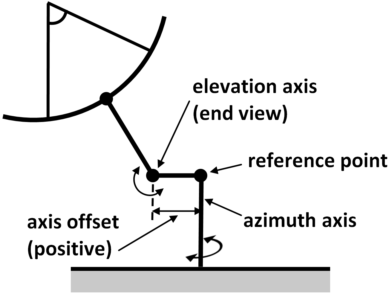
(a) Alt-azimuth mount with a positive axis offset

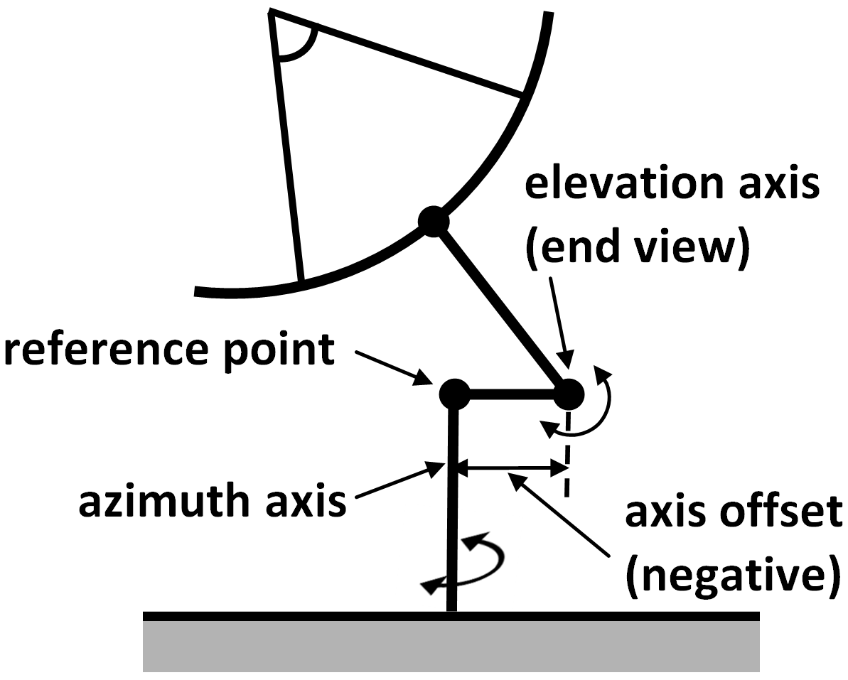
(b) Alt-azimuth mount with a negative axis offset

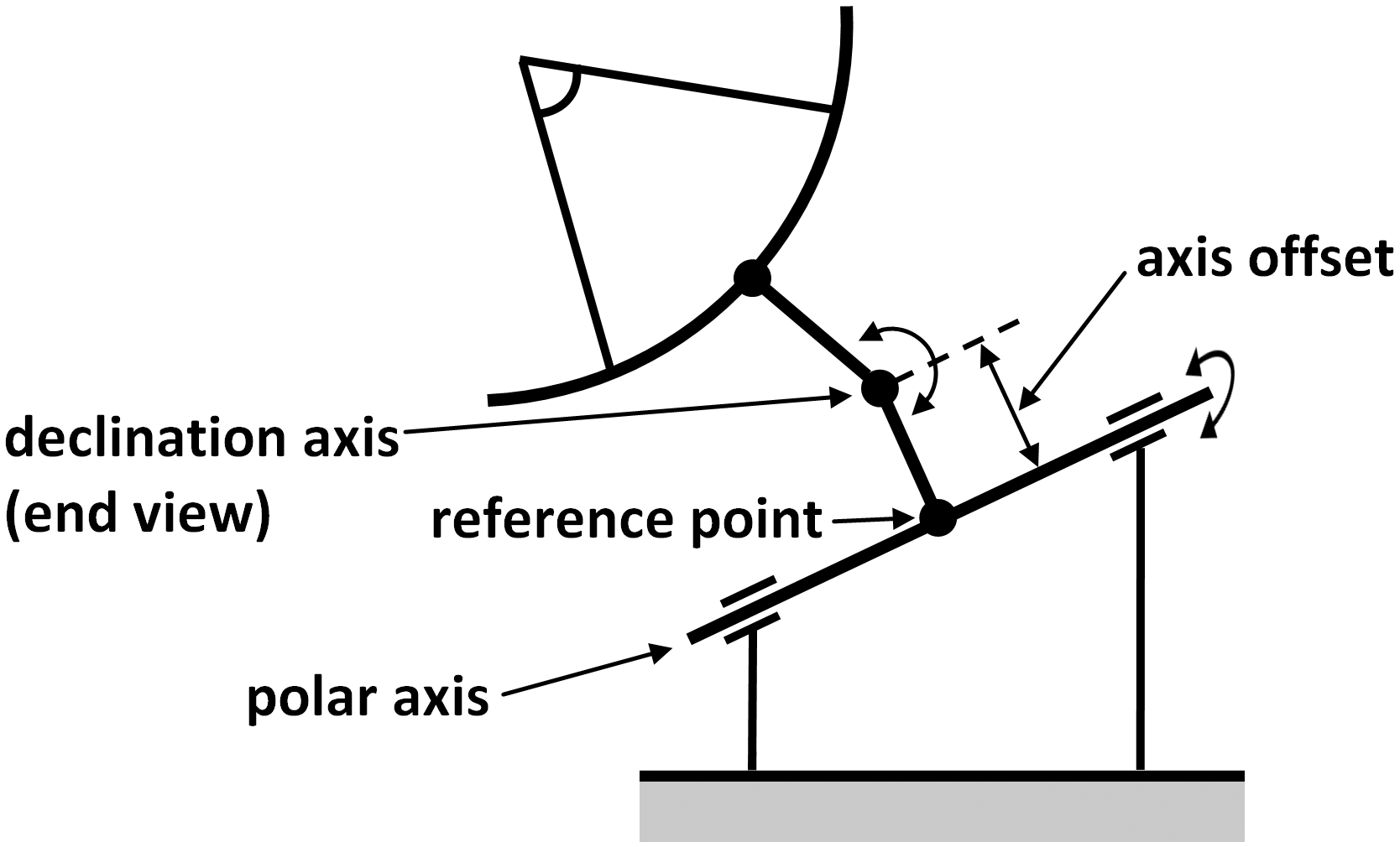
(c) Polar mount

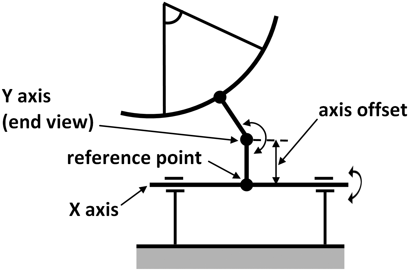
(d) X-Y mount

Figure 1: Common mount types of ground steerable high-gain antennas.

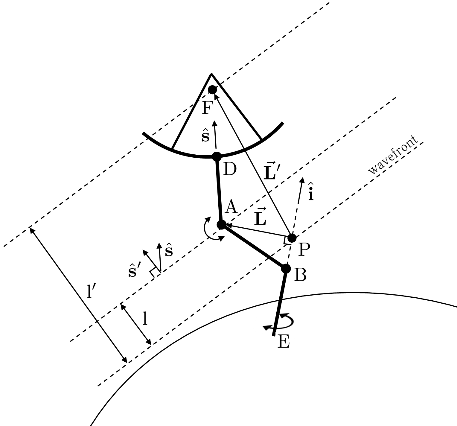
Figure 2: Generic mount of a ground steerable high-gain antenna. Dashed lines mark the positions of the wavefront at the moments of its passing through the antenna focus, $F$, antenna rotation axis $A$, and the antenna reference point, $P$.

Let us now consider a generalized antenna structure that encompasses all the three antenna mounts described above (Fig. 2). The antenna has two perpendicular rotation axes: $BE$, which is fixed relative to the Earth, and $A$ (end-view), which is movable. The Earth-fixed antenna reference point, $P$, used to refer all the incoming/outgoing signals to, is usually chosen on axis $BE$ and defined as its intersection with the plane that is perpendicular to $BE$ and contains axis $A$. If the two axes intersect then $P$ is simply the intersection point of the axes. Let us further introduce the unit vector $\hat{\mathbf{s}}$ along the antenna symmetry axis, $AD$, the unit vector $\hat{\mathbf{i}}$ along axis $BE$, and the unit vector $\hat{\mathbf{s}}^{\prime}$ in the direction of propagation of the wavefront, which we assume to be plane. (We ignore the wavefront curvature according to (Sovers et al., 1998).) Finally, we define the axis separation vector $\mathbf{L}=\overrightarrow{PA}$, denote the antenna focus by $F$, and introduce $\mathbf{L^{\prime}}=\overrightarrow{PF}$.

The influence of the antenna motion on the parameters of received and transmitted signals, such as phase, frequency, and time of arrival can be easily understood from Fig. 2. Without loss of generality let us consider the case of the antenna receiving a signal from a SC and assume a prime focus antenna construction. While the received signal characteristics are referred to the Earth-fixed reference point $P$, in reality the wavefront first reaches the movable antenna dish surface, then travels a fixed-length path to the focus, $F$, and then passes along waveguides and cables, again of fixed length, to the data acqusition equipment. (As noted above, we neglect the environmental effects.) The fixed-length parts of the signal path in the antenna structure, waveguides, cabling, and equipment delays can usually be neglected, both in VLBI and SC tracking, since they add constant offsets to the signal phase and delay and do not influence the frequency (Sovers et al., 1998). It is the variation of the distance between the positions of the wavefront at the moments when it passes through points $F$ and $P$, which we denote by $l^{\prime}$, that gives a variable contribution to the measured signal characteristics. Obviously, we have

$$l^{\prime}=\hat{\mathbf{s}}^{\prime}\cdot\mathbf{L^{\prime}},$$ (1)

where $\mathbf{L^{\prime}}=\overrightarrow{PF}$. Note that in general $\hat{\mathbf{s}}^{\prime}$ does not lie in the plane of vectors $\hat{\mathbf{s}}$ and $\mathbf{L}$ since both of the antenna pointing angles, e.g. elevation and azimuth, may be in error.

Eq. (1) gives a general expression for the length of that part of the signal path which varies due to the antenna motion. The respective general expressions for the extra phase delay, $\tau^{\prime}$, and the fractional frequency shift, $\Delta f/f$, are:

$$\tau^{\prime}=\frac{l^{\prime}}{c}=\frac{\hat{\mathbf{s}}^{\prime}\cdot\mathbf{L^{\prime}}}{c},$$ (2)

$$\frac{\Delta f}{f}=-\frac{1}{c}\frac{d}{dt}(\hat{\mathbf{s}}^{\prime}\cdot\mathbf{L^{\prime}}).$$ (3)

Let us now consider the simplified case of negligible pointing errors:

$$\hat{\mathbf{s}}=\hat{\mathbf{s}}^{\prime}.$$ (4)

In this case it is easy to see that Eqs. (2) and (3) reduce to their unprimed analogues familiar from previous analyses (Sovers et al., 1998):

$$\tau=\frac{l}{c}=\frac{\hat{\mathbf{s}}\cdot\mathbf{L}}{c},$$ (5)

$$\frac{\Delta f}{f}=-\frac{1}{c}\frac{d}{dt}(\hat{\mathbf{s}}\cdot\mathbf{L}),$$ (6)

where $l$ is the distance between the wavefront positions at the moments when it passes through axis $A$ and point $P$:

$$l=\hat{\mathbf{s}}\cdot\mathbf{L}.$$ (7)

Indeed, if $\hat{\mathbf{s}}=\hat{\mathbf{s}}^{\prime}$ we have:

$$\begin{split}l^{\prime}&=\hat{\mathbf{s}}\cdot\left(\mathbf{L}+\overrightarrow{AF}\right)\\ &=l+AF,\end{split}$$ (8)

so that $l$ and $l^{\prime}$ differ only by a constant term of $AF$ which results in a constant phase delay term in Eq. (2) and does not contribute to the frequency shift of Eq. (3).

Simple geometric considerations lead to the following useful equation for the axis separation vector, which is independent of the assumption of $\hat{\mathbf{s}}=\hat{\mathbf{s}}^{\prime}$:

$$\mathbf{L}=\pm L\frac{\hat{\mathbf{i}}\times(\hat{\mathbf{s}}\times\hat{\mathbf{i}})}{\big{|}\hat{\mathbf{i}}\times(\hat{\mathbf{s}}\times\hat{\mathbf{i}})\big{|}}.$$ (9)

Here, $L=|\mathbf{L}|$ and the plus sign is used for “positive” offset antennas (such that when $\hat{\mathbf{s}}$ and $\mathbf{L}$ are parallel or antiparallel the antenna comes closer to the source as $L$ increases, e.g. as in Fig. 1a) and minus for “negative” offset antennas (vice versa, e.g. as in Fig. 1b). Let us return to the case of $\hat{\mathbf{s}}=\hat{\mathbf{s}}^{\prime}$. Using Eqs. (7) and (9), as well as the geometric relation of

$$\hat{\mathbf{i}}\times(\hat{\mathbf{s}}\times\hat{\mathbf{i}})=\hat{\mathbf{s}}-\hat{\mathbf{i}}(\hat{\mathbf{i}}\cdot\hat{\mathbf{s}}),$$ (10)

it is straightforward to obtain the following well-known equation for

$$l=\pm L\sqrt{1-(\hat{\mathbf{s}}\cdot\hat{\mathbf{i}})^{2}}=\pm L\cos\theta,$$ (11)

where we denoted

$$\theta=\frac{\pi}{2}-\angle(\hat{\mathbf{s}},\hat{\mathbf{i}}).$$ (12)

For the three antenna mounts discussed above, alt-az, polar, and X-Y, this angle is, respectively, elevation, declination, and auxiliary angle $Y$.

The assumption of $\hat{\mathbf{s}}=\hat{\mathbf{s}}^{\prime}$ is usually valid to a very good degree for the case of tracking celestial objects with well known coordinates. However, it can easily fail when tracking SC. Indeed, the accuracy of predicted orbits used for tracking SVLBI spacecraft can be as low as 5 km for each component of the position vector, which corresponds to $\angle(\hat{\mathbf{s}},\hat{\mathbf{s}}^{\prime})\sim 17^{\prime}$ for the distance to the SC of $\sim 1,000$ km (Zakhvatkin et al., 2020). When a ground TS is receiving signals sent by a SC, its antenna operators usually can partially compensate for the inaccuracy of the predicted orbit by applying constant pointing offsets that maximize the level of the received signal. However, this does not eliminate the pointing error completely (e.g. when it changes during the communication session) and such procedure cannot be performed when the TS is transmitting signals to the SC. It seems reasonable to assume that the pointing error is at least of the order that corresponds to the accuracy of the reconstructed SC orbit. For RadioAstron the accuracy of the reconstructed orbit near perigee is $\sim 100$ m for each component of the position vector, which corresponds to $\angle(\hat{\mathbf{s}},\hat{\mathbf{s}}^{\prime})\sim 20^{\prime\prime}$ at the distance to the SC of $\sim 1,000$ km (see Section 3.2). This pointing error is usually larger for the SC-mounted antenna since there is no operator on board to apply pointing corrections and also because predicted orbits used by spacecraft are often uploaded to the on-board computer a few days in advance of the communication sessions and thus are less up-to-date and less accurate than those used by ground antennas. Moreover, at least for RadioAstron, pointing angles for the onboard antenna are computed on the fly by the on-board computer based on simplified models of the spacecraft motion and signal propagation.

Now, let us consider the practically important case when

$$\hat{\mathbf{s}}\neq\hat{\mathbf{s}}^{\prime}$$ (13)

but the pointing errors are small. If we introduce the pointing error vector of

$$\delta\mathbf{s}=\hat{\mathbf{s}}^{\prime}-\hat{\mathbf{s}},$$ (14)

the assumption of small pointing errors can be stated as:

$$|\delta\mathbf{s}|\ll 1.$$ (15)

Note that, since $|\hat{\mathbf{s}}^{\prime}|=|\hat{\mathbf{s}}|=1$, we have:

$$\begin{split}\delta\mathbf{s}\cdot\hat{\mathbf{s}}^{\prime}=O(\delta\mathbf{s}^{2}),\\ \delta\mathbf{s}\cdot\hat{\mathbf{s}}=O(\delta\mathbf{s}^{2}).\end{split}$$ (16)

Substituting $\hat{\mathbf{s}}=\hat{\mathbf{s}}^{\prime}-\delta\mathbf{s}$ into Eq. (1) and expanding it in powers of $\delta\mathbf{s}$, and also using Eq. (16) and $\mathbf{L^{\prime}}=\mathbf{L}+\overrightarrow{AF}$, it is straightforward to obtain:

$$\begin{split}l^{\prime}&=\pm L\cos\theta^{\prime}+O(\delta\mathbf{s}^{2})\\ &=\pm L\cos\theta^{\prime}+O(\delta\mathbf{\theta}^{2}),\end{split}$$ (17)

where

$$\theta^{\prime}=\frac{\pi}{2}-\angle(\hat{\mathbf{s}}^{\prime},\hat{\mathbf{i}})$$ (18)

is the “true” elevation, declination, or auxiliary angle $Y$ of the SC relative to the ground antenna (respectively, for the alt-az, polar, and X-Y mounts) and $\delta\theta$ is the error in this angle:

$$\delta\theta=\theta^{\prime}-\theta.$$ (19)

Although Eqs. (11) and (17) formally look similar, their meaning is different. In Eq. (11) $\theta$ is the angle determined by the antenna pointing direction, $\hat{\mathbf{s}}$, while in Eq. (17) $\theta^{\prime}$ is determined by the actual source/target position relative to the antenna, $\hat{\mathbf{s}}^{\prime}$. Also, while Eq. (11) is exact, Eq. (17) is valid only for small pointing errors.

The expression for the fractional frequency shift due to the APCM effect can be obtained from Eq. (17) using Eq. (3) and assuming the rate of change of the $O(\delta\mathbf{\theta}^{2})$ term is small, i.e. $\frac{d}{dt}O(\delta\mathbf{\theta}^{2})=O(\delta\mathbf{\theta}^{2})$. Thus we have:

$$\frac{\Delta f}{f}=\pm\frac{L}{c}\dot{\theta}^{\prime}\sin\theta^{\prime}+O(\delta\mathbf{\theta}^{2}),$$ (20)

where the plus sign is for “positive” offset antennas and minus for the “negative” (as above).

The equations for the extra phase delay and fractional frequency shift for the three common antenna mounts are summarized in Table 1.

Antenna mount	Secondary angle	Delay correction, $\tau^{\prime}$	Frequency correction, $\Delta f/f$
alt-az	elevation $\gamma^{\prime}$	$\pm(L/c)\cos{\gamma^{\prime}}$	$\pm\;\;\;(L/c)\;\dot{\gamma}^{\prime}\sin\gamma^{\prime}$
polar	declination $\delta^{\prime}$	$\pm(L/c)\,\cos{\delta^{\prime}}$	$\pm\;\;\;(L/c)\;\dot{\delta}^{\prime}\sin\delta^{\prime}$
X-Y	auxiliary angle $Y^{\prime}$	$\pm(L/c)\,\cos{Y^{\prime}}$	$\pm\;\;\;(L/c)\;\dot{Y}^{\prime}\sin Y^{\prime}$

Table 1: Equations to compute the antenna phase center motion effect for common antenna mounts. The upper sign is for “positive” axis offset antennas while the lower one, respectively, for the negative (see the text for details).

2.2 Spaceborne antennas

Let us now consider SC-mounted antennas. The equations for the APCM effect for spaceborne antennas are obtained relatively straightforwardly and in close analogy to the case of ground antennas. The description of the SC motion is usually given in terms of the position of its center of mass, point $C$ on Fig. 3, and its attitude in a selected reference frame. For Earth-orbiting SC an Earth-centered inertial reference frame is usually used, e.g. EME2000. The center of mass, $C$, also serves as the antenna reference point, i.e. the characteristics of the signals received and/or transmitted by the antenna are referred to this point. An insignificant difference from ground antenna mounts is that in this case it is $AB$ that usually serves as one of the two antenna axes instead of $BE$. The other axis is oriented normal to the plane of Fig. 3 and located at the axis intersection point $A$.

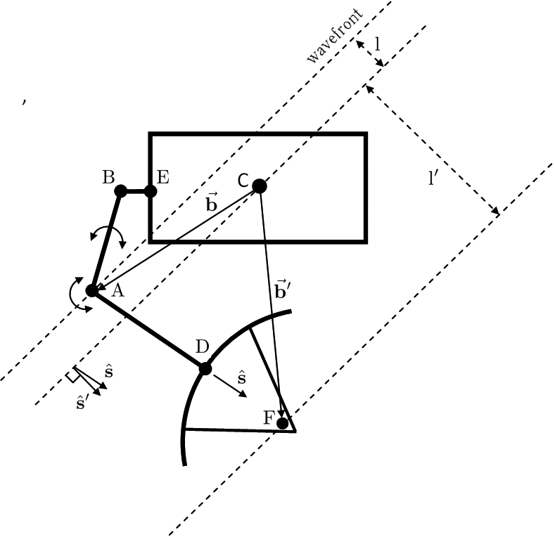
Figure 3: Generic spacecraft steerable high-gain antenna mount. Dashed lines mark the positions of the wavefront at the moments of its passing through the antenna focus, $F$, the antenna axis intersection point, $A$, and the spacecraft center of mass, $C$, which also serves as the antenna reference point.

Now, we define the unit vector $\hat{\mathbf{s}}^{\prime}$ in the direction of the source/target, i.e. normal to the wavefront (which we again consider to be plane), the unit vector $\hat{\mathbf{s}}$ in the direction of the antenna symmetry axis, $AD$, the displacement vector of the antenna primary focus from the center of mass, $\overrightarrow{CF}=\mathbf{b^{\prime}}$, and a similar displacement vector for the axes intersection point, $A$: $\overrightarrow{CA}=\mathbf{b}$. In analogy to the ground case, the APCM effect is determined by the variable distance between the positions of the wavefront at the moments of its passing through the antenna focus, $F$, and the reference point, $C$:

$$l^{\prime}=\mathbf{b^{\prime}}\cdot\hat{\mathbf{s}}^{\prime}.$$ (21)

Also similar to the ground case, when the pointing errors can be neglected, i.e. $\hat{\mathbf{s}}^{\prime}=\hat{\mathbf{s}}$, we can use $\mathbf{b^{\prime}}=\mathbf{b}+\overrightarrow{AF}$ and $\overrightarrow{AF}=AF\cdot\hat{\mathbf{s}}$ to obtain:

$$l^{\prime}=l+\mathrm{const},$$ (22)

where $l$ is the distance travelled by the wavefront between its positions when passing through the axis intersection point, $A$, and the center of mass, $C$:

$$l=\mathbf{b}\cdot\hat{\mathbf{s}}.$$ (23)

If there are small pointing errors:

$$|\delta\mathbf{s}|=|\hat{\mathbf{s}}^{\prime}-\hat{\mathbf{s}}|\ll 1,$$ (24)

it is straightforward to show that Eq. (21), again in analogy with the ground case, simplifies to:

$$l^{\prime}=\mathbf{b}\cdot\hat{\mathbf{s}}^{\prime}+\mathrm{const}+O(\delta\mathbf{s}^{2}).$$ (25)

The advantage of this equation over Eq. (21) is that vector $\mathbf{b}$ is fixed in the spacecraft reference frame while vector $\mathbf{b^{\prime}}$ moves according to the antenna motion.

The generic expression for the fractional frequency shift of the signal received or transmitted by the SC antenna can be obtained from Eq. (21) using Eq. (3):

$$\frac{\Delta f}{f}=-\frac{1}{c}\frac{d}{dt}(\mathbf{b^{\prime}}\cdot\hat{\mathbf{s}}^{\prime}).$$ (26)

For small pointing errors we have:

$$\frac{\Delta f}{f}=-\frac{1}{c}\frac{d}{dt}(\mathbf{b}\cdot\hat{\mathbf{s}}^{\prime})+O(\delta\mathbf{s}^{2}),$$ (27)

where we again assumed that the rate of change of $O(\delta\mathbf{s}^{2})$ terms in Eq. (25) is small. In many cases, e.g. in SVLBI, the spacecraft maintains constant attitude in an inertial reference frame when communicating with a TS. In this case vector $\mathbf{b}$ is constant in an inertial reference frame and Eq. (27) further simplifies to:

$$\frac{\Delta f}{f}=-\frac{1}{c}(\mathbf{b}\cdot\dot{\hat{\mathbf{s}}}^{\prime})+O(\delta\mathbf{s}^{2}).$$ (28)

For numerical computations of the APCM effect, as well as its uncertainties, it is useful to specify vector $\mathbf{b}$ in the SC-fixed reference frame, which we denote by $\mathbf{b}_{\mathrm{sc}}$, while vector $\hat{\mathbf{s}}^{\prime}$ is more naturally defined in the inertial reference frame. Denoting the transformation matrix from the SC-fixed to the inertial frame by $\mathrm{R}$, we obtain the following equation for the APCM effect due to the SC antenna (assuming a constant SC attitude in the inertial frame):

$$\frac{\Delta f}{f}=-\frac{1}{c}(\mathrm{R}\mathbf{b}_{\mathrm{sc}}\cdot\dot{\hat{\mathbf{s}}}^{\prime})+O(\delta\mathbf{s}^{2}).$$ (29)

2.3 Error analysis

In high-accuracy experiments we are interested not only in the magnitude of the APCM effect but also in estimating the errors in its computed values. The errors can be assessed using equations obtained above by varying them with respect to the particular parameters. For example, the error in the fractional frequency shift of Eq. (29) due to an error, $\delta\mathbf{b}_{\mathrm{sc}}$, in the position of the fixed SC antenna axis relative to the SC center of mass is:

$$\delta\left(\frac{\Delta f}{f}\right)=-\frac{1}{c}((\mathrm{R}\,\delta\mathbf{b}_{\mathrm{sc}})\cdot\dot{\hat{\mathbf{s}}}^{\prime})+O(\delta\mathbf{s}^{2}).$$ (30)

Then, for the uncertainty in the fractional frequency shift due to the APCM effect, which we will characterize by the standard deviation, we have:

$$\sigma_{\Delta f/f}=\left(\frac{1}{c^{2}}(\dot{\hat{\mathbf{s}}}^{\prime})^{\mathrm{T}}\mathrm{R}\Sigma_{b}\mathrm{R}^{\mathrm{T}}\dot{\hat{\mathbf{s}}}^{\prime}+...\right)^{1/2}+O(\delta\mathbf{s}^{2}),$$ (31)

Error source	Affected parameter	RadioAstron	Possible follow-up SVLBI mission
Uncertainty in the offset between the ground antenna axes	$L$	0.002 m	0.002 m
Ground antenna axis misalignment	$\hat{\mathbf{i}}$	5′	5′
Uncertainty in the position of the intersection point of the SC antenna axes relative to the SC center of mass	$\mathbf{b}_{\mathrm{sc}}$	0.005 m	0.001 m
Uncertainty in the SC attitude	$\mathrm{R}$	10′′	1′′
Uncertainty in the TS-to-SC direction due to the SC position uncertainty	$\hat{\mathbf{s}}$	100m $\rightarrow$ 20′′	10m $\rightarrow$ 2′′

Table 2: Uncertainties in the parameters that affect the computed phase and frequency shift due to the antenna phase center motion effect. Two sets of values are given: one is relevant for RadioAstron and the other is a set of tentative values assumed for a possible follow-up SVLBI mission. For the unit vector along the ground antenna fixed axis, $\hat{\mathbf{i}}$, and the unit vector in the TS-to-SC direction, $\hat{\mathbf{s}}$, the uncertainties in each of the two angles that define the orientation of these vectors are specified. The uncertainties in the direction of $\hat{\mathbf{s}}$ are computed from the specified average uncertainties in the components of the SC position vector, assuming a distance to the TS of 1,000 km. For the on-board antenna axis position vector, $\mathbf{b}$, the uncertainty in each of its three components is specified. For the transformation matrix, $\mathrm{R}$, the uncertainty in each of the three angles that define its components are specified. In all cases the specified uncertainties in vector components and angles are assumed independent.

where $\Sigma_{b}$ is the variance-covariance matrix of the components of vector $\mathbf{b}_{\mathrm{sc}}$ and the ellipsis denotes similar terms due to other parameters, which we assumed to be independent from $\mathbf{b}_{\mathrm{sc}}$.

The rate of change of the TS-to-SC direction vector, $\hat{\mathbf{s}}^{\prime}$, significantly depends on the orbit parameters, the TS location, and the SC position on the orbit. Therefore, an error analysis of the APCM effect should be performed for each mission individually, taking into account its configuration and the particular values of uncertainties in the parameters. Moreover, it is necessary to characterize $\sigma_{\Delta f/f}$ not with a single, e.g. maximum, value but as a function of the SC position on its orbit.

In the next two sections we outline the results of two such error analyses based on Eq. (31) and a similar equation for the uncertainty in the ground APCM effect (which can be straightforwardly obtained from Eq. (3) or (20)): one for the RadioAstron SC and another for a SC of a possible follow-up SVLBI mission. Section 3 can also serve as a rather detailed account of the part of the error budget of the RadioAstron gravitational redshift experiment (Litvinov et al., 2018; Nunes et al., 2020) which is relevant to the APCM effect. For simplicity we consider only some of the possible error sources, see Table 2, and treat each of the listed parameter as independent. We also assume each component of the vector parameters to be independent. The particular values given in Table 2 are commented on in the next Section.

3 The APCM effect in the RadioAstron SVLBI mission

3.1 The RadioAstron spacecraft

The RadioAstron spacecraft served the RadioAstron SVLBI mission from 2011 to 2019 and helped astronomers observe various astrophysical objects at the highest angular resolution to date (Kardashev et al., 2013; Johnson et al., 2016; Giovannini et al., 2018; Kravchenko et al., 2020). In 2019 the spacecraft stopped responding to commands and the observational part of the mission ended. The satellite is on a highly eccentric orbit around the Earth which was designed to evolve significantly throughout the mission under the gravitational influence of the Moon, as well as other factors, within a broad range of the orbital parameter space (perigee altitude 1,000–82,000 km, apogee altitude 273,000–357,000 km, period 8.2–10.2 day, Figs. 4 and 5).

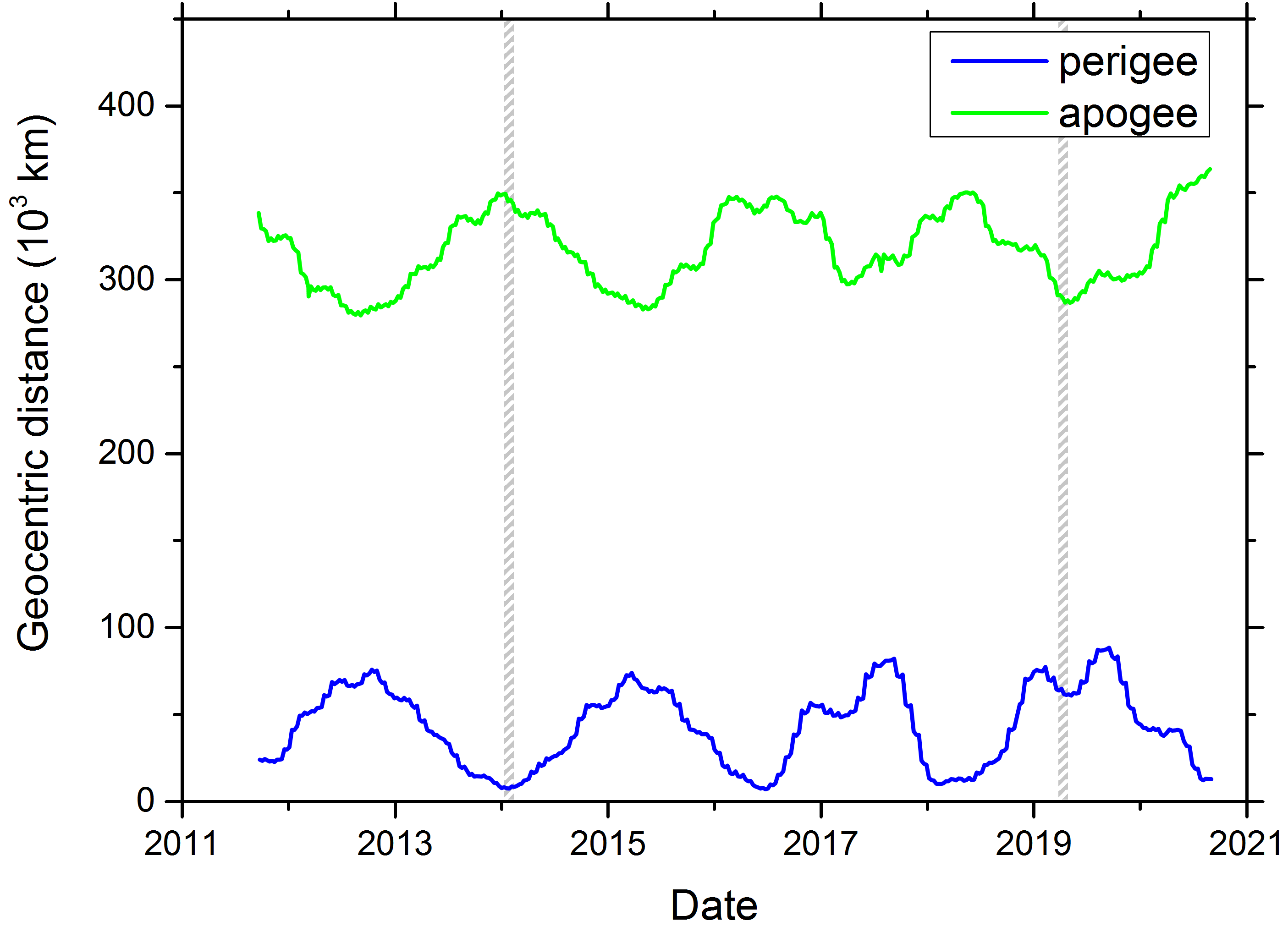
Figure 4: Evolution of the apogee and perigee of the RadioAstron spacecraft. The evolution of the orbit is caused largely by the gravitational interaction with the Moon. The two segments used in the analyses of Sections 3.3 and 5 are hatched.

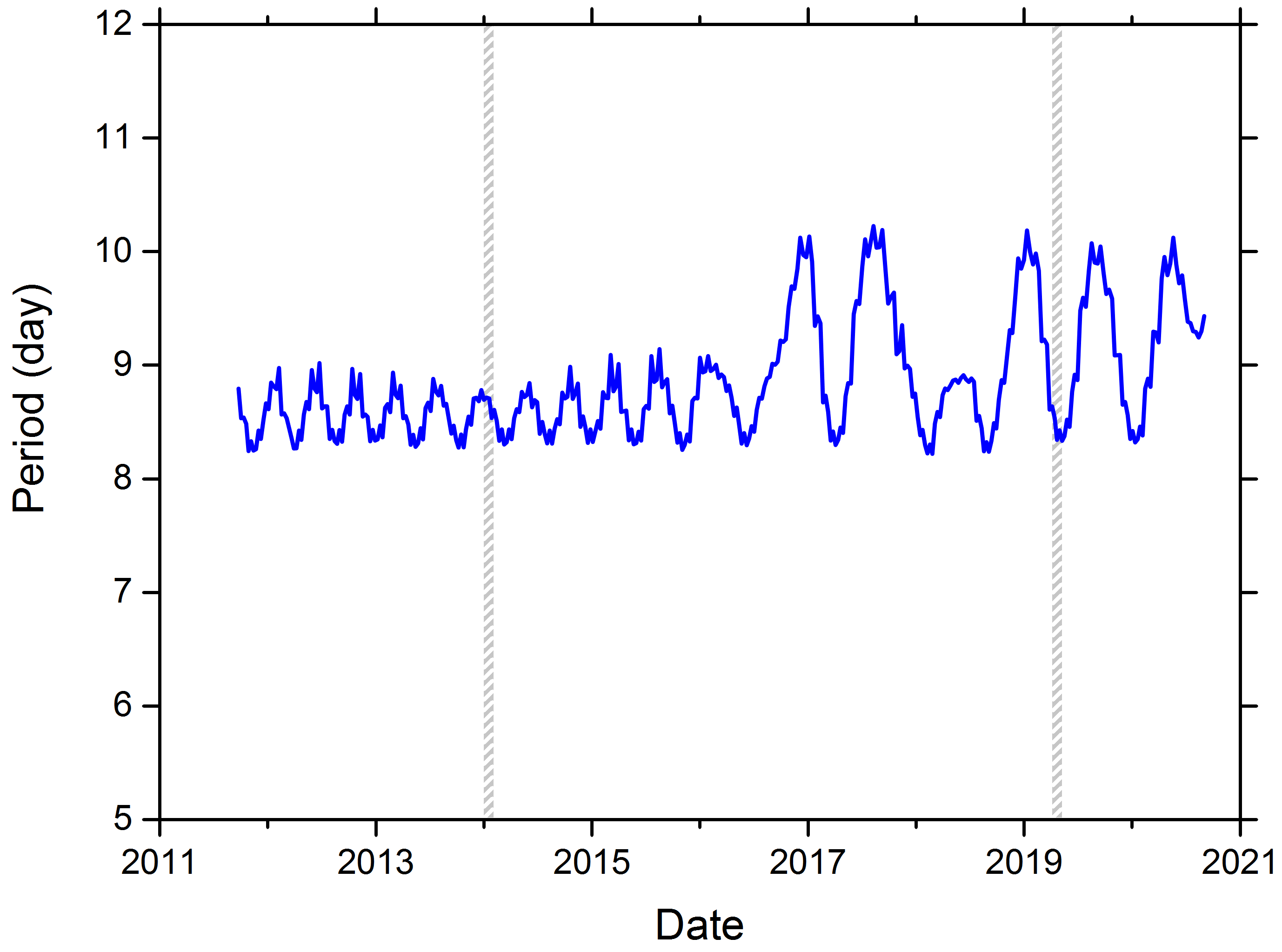
Figure 5: Evolution of the period of the RadioAstron spacecraft. The irregular low spike in 2018 is caused by an orbital maneuver applied to avoid colliding with the Earth. The two segments used in the analyses of Sections 3.3 and 5 are hatched.

The SC is equipped with five antennas: 1) one 10-meter high-gain parabolic spacecraft-fixed antenna used for observing celestial sources; 2) one 1.5m high-gain parabolic mechanically steerable antenna for a) transmitting high-bit-rate observational data to the Earth, b) transmitting the highly stable signal of the on-board hydrogen maser frequency standard to the Earth for the purpose of Doppler tracking, and c) receiving a stable signal from an Earth-based hydrogen maser for use as a reference on board (backup mode); 3) three omnidirectional antennas for transmitting telemetry, receiving commands, Doppler and range tracking. The antenna of interest to us is the 1.5 m high-gain steerable antenna (Fig. 6).

This antenna communicated with the mission’s two ground TS that were used to collect science data, receive one- and two-way Doppler, and also to provide uplink reference signal for the spacecraft. The mission’s two tracking stations were the Pushchino TS of the Pushchino Radio Astronomy Observatory (Moscow region, Russia) with its 22m alt-az mount radio telescope RT-22 and the Green Bank Earth Station of the National Radio Astronomy Observatory (West Virginia, US) with its 43-meter NRAO140 polar mount radio telescope. The parameters of these two antennas are given in Table 3.

3.2 Description of the data, error sources, and data processing

According to the equations derived in Section 2, to compute the APCM effect both for the ground and space antennas the following data are needed: the SC orbit, the position of the SC-fixed antenna axis relative to its center of mass, the SC attitude as a function of time, the coordinates of the ground an- tenna,   and   its   axis   offset.   The information   on   the   actual

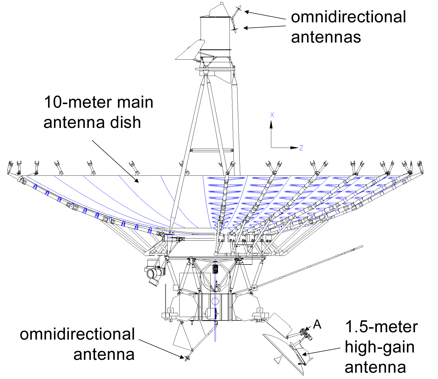
Figure 6: A technical drawing of the RadioAstron spacecraft (Fedorchuk & Arkhipov, 2014). The spacecraft is equipped with several antennas, the largest of which is the 10-meter spacecraft-fixed parabolic dish used in astronomical observations. The antenna of interest to us is the 1.5-meter high-gain mechanically steerable antenna. Point $A$ marks the intersection of the rotation axes of this antenna.

pointing of the antennas during communication sessions is not needed as long as pointing errors are small.

In our analysis we use long-term predicted orbits provided for the RadioAstron mission by the ballistic center of the Keldysh Institute for Applied Mathematics (KIAM) (Zakhvatkin et al., 2020). Orbits of this type were produced primarily for the purpose of long-term planning of the mission operations. For a prediction time of about a month the average uncertainties in each component of the SC position and velocity vectors of such orbits can reach, correspondingly, 10 km and several cm/s. (These uncertainties are distributed unevenly between the vector components along and across the line of sight.) The KIAM also provides significantly more accurate aposteriori reconstructed orbits with average uncertainties in each component of the position and velocity vectors of $\sim$200 m and 2–3 mm/s, correspondingly. (These uncertainties are distributed relatively evenly between the vector components and also depend on the distance to the SC: near perigees the uncertainty in the SC position is usually several times lower than near apogees while that in the velocity is correspondingly larger.) In this paper we do not use reconstructed orbits to compute the APCM effect because orbits of this type are available only for the time segments when observations were performed and also because the accuracy of long-term predicted orbits is sufficient for our illustrative purposes. However, since in the data processing of experiments performed with RadioAstron one uses reconstructed orbits, we estimate the uncertainty in the TS-to-SC direction, $\hat{\mathbf{s}}^{\prime}$, using the SC position uncertainty relevant to reconstructed orbits. For simplicity, we use a single value for the uncertainties in each of the two angles that determine the TS-to-SC direction and estimate it using the average uncertainty in the SC position that is relevant to perigees, i.e. 100 m (see Table 2).

	Pushchino	Green Bank
Location	Moscow region, Russia	West Virginia, USA
Latitude	54∘49.0′14.24	+38∘26′16.166′′
Longitude	37∘37′41.84′′	-79∘50′08.810′′
Height	239.09 m	812.50 m
Dish diameter	22 m	43 m
Mount type	alt-az	polar
Axis offset	0.0 m	14.94 m

Table 3: Parameters of the antennas of the two tracking stations of the RadioAstron mission.

In order to compute the components of the displacement of the intersection point of the SC rotation axes off the SC center of mass, $\mathbf{b}$, we determined the coordinates of that point from a high-resolution technical drawing version of Fig. 6, while the position of the SC center of mass was obtained from internal technical documentation of the RadioAstron mission. The location of the center of mass depends on the amount of fuel in the tank, which for simplicity we assumed to be full. Thus we obtained:

$$\mathbf{b}_{\mathrm{sc}}=\left[-2.299;\>0;\>2.546\right]~{}\mathrm{m}.$$ (32)

The rigidity properties of the antenna mount construction and the accuracy of the position of the center of mass make it reasonable to attribute an uncertainty of $\sim 5$ mm to each component of vector $\mathbf{b}_{\mathrm{sc}}$ (Table 2).

Eq. (32) gives the components of vector $\mathbf{b}$ in the SC-fixed reference frame. In order to transform them to an inertial reference frame using the transformation matrix $\mathrm{R}$, see Eq. (29), the knowledge of the SC attitude as a function of time is required. The SC attitude during a particular observation almost always was maintained constant but it differed from one observation to another (the duration of an observation was usually of order of an hour). For the actual data processing the information on the SC attitude is obtained from the telemetry data provided by the on-board attitude control system. The accuracy of these data, obtained mostly from RadioAstron’s star trackers, corresponds to the uncertainty in each of the three angles that determine the SC orientation of $\sim 10^{\prime\prime}$ (Table 2). For our illustrative purposes we assume the SC always maintains a constant orientation in the inertial space, such that the transformation between the two reference frames is represented by the identity matrix, $\mathrm{R}=1$. However, we allow for an error in the realization of this orientation by the attitude control system, $\delta\mathrm{R}$, and estimate it using the above uncertainties in the orientation angles (assumed independent from each other).

The geodetic (ITRS) coordinates of the reference point of the Pushchino RT-22 antenna and its axis offset were obtained from internal documentation of the RadioAstron mission, while those of the NRAO140 antenna from (Langston, 2012). The uncertainties in the antenna reference point coordinates are of order of a cm and thus give negligible contribution to the uncertainty in the TS-to-SC direction compared to that of the SC position. The uncertainties in the axis offsets were assumed to be 2 mm based on the difference between the value provided in (Langston, 2012) and that obtained from data processing of global geodetic VLBI campaigns (Petrov, 2009).

Finally, we take into account the possibility for a small misalignment of the Earth-fixed axis of the ground antenna from its intended direction. For example, for an alt-az antenna its azimuth axis may be slightly offset from the true local zenith, for a polar mount antenna its polar axis may not point exactly along the Earth’s rotation axis. This error is reflected by an error in the direction of vector $\hat{\mathbf{i}}$ for which we assume a value of 5^′. This value is very tentative and corresponds to the misalignment of the electrical and mechanical axes of the NRAO140 antenna (Mezger et al., 1966). Antenna pointing calibrations can probably reduce it by at least half an order of magnitude.

The computation of the APCM effect for the ground and space antennas of the RadioAstron mission involves direct application of equations of Section 2. The errors are estimated according to Section 2.3.

3.3 Results

Due to the highly evolving character of RadioAstron’s orbit, we selected two distinct epochs for our analysis: a low-perigee epoch of January 2014 and a high-perigee epoch of April 2019. Some of the orbital parameters relevant to these two epochs, which we denote, respectively, A and B, are given in Table 4.

	Epoch A: Jan 2014	Epoch B: Apr 2019
Perigee (km)	7,361	64,745
Apogee (km)	345,060	286,804
Period (day)	8.6	8.5
Eccentricity	0.96	0.63

Table 4: The orbital parameters of the RadioAstron spacecraft for the two selected epochs of low (A) and high (B) perigee.

We computed the ground APCM effect only for the Green Bank NRAO140 antenna since the Pushchino antenna formally has a zero axis offset and thus does not exhibit it. For both selected epochs we show the evolution of the effect and its errors over a time span of approximately 1.5 orbital revolutions and a zoomed-in view into one of the perigees. The results are presented in Figs. 7–10.

Several aspects of these results are worth noting. First, since the effect and its errors vary over many orders of magnitude, we use a logarithmic scale which allows us to plot only the absolute values of the effect. This results in the many visible dips which are merely due to the effect changing its sign. Second, the curves are plotted even for the time segments when the SC was below the horizon for NRAO140 or the tracking constraints for the ground or space antenna were not met. This is done for the sake of visual clarity and because the particular SC visibility conditions and tracking constraints are affected in a semi-random way by the interplay of the particular values of the SC orbital parameters. It is worth noting, however, that the SC was visible to NRAO140 near and at the top of the spikes of the APCM effect in Fig. 7. An example of the data processing of a series of experiments performed near one of those spikes is presented below in Fig. 11. Another important observation is that the magnitudes of the space and ground effects are comparable. Further, as expected, near perigees the effect is larger in epoch $A$ than in $B$, by an order of magnitude, due to the more rapid motion of the SC across the sky. However, outside the near-perigee regions the situation is usually opposite, i.e. the effect is larger in epoch $B$ than in $A$, also by an order of magnitude. For each epoch both the ground and SC effects are larger than $10^{-13}$ on significant parts of the orbit and almost never fall below $10^{-14}$ in the high-perigee epoch.

The correction to the ground antenna effect implied by Eq. (20), that is, the necessity to use $\theta^{\prime}$ computed from the true TS-to-SC direction instead of the respective antenna pointing angle, $\theta$, is larger than $1\times 10^{-14}$ on some parts of the orbit and thus is significant for high-accuracy SC tracking experiments.

The errors of estimating the APCM effect are more significant near perigees as well. The largest are due to the SC antenna axis position uncertainty, ground antenna axis misalignment and the ground antenna axis offset.

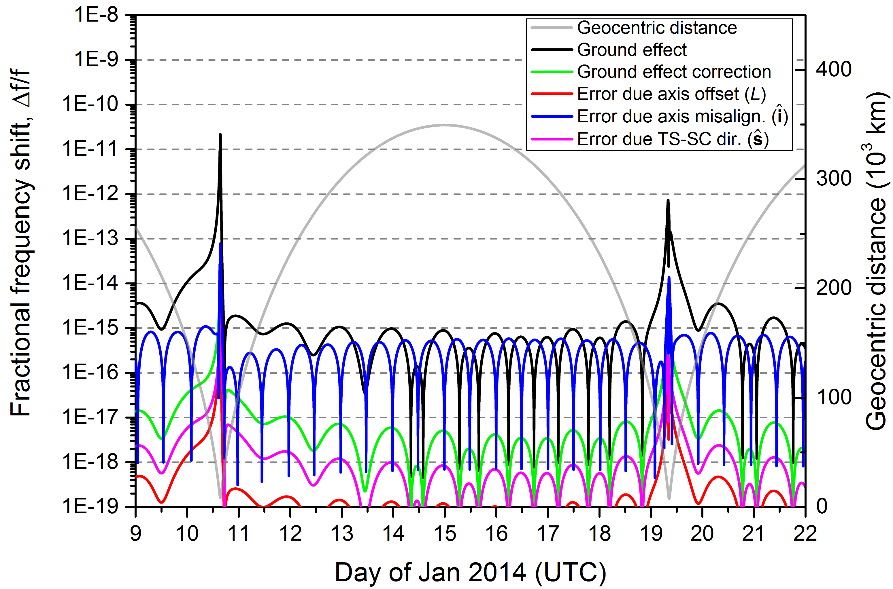
(a)

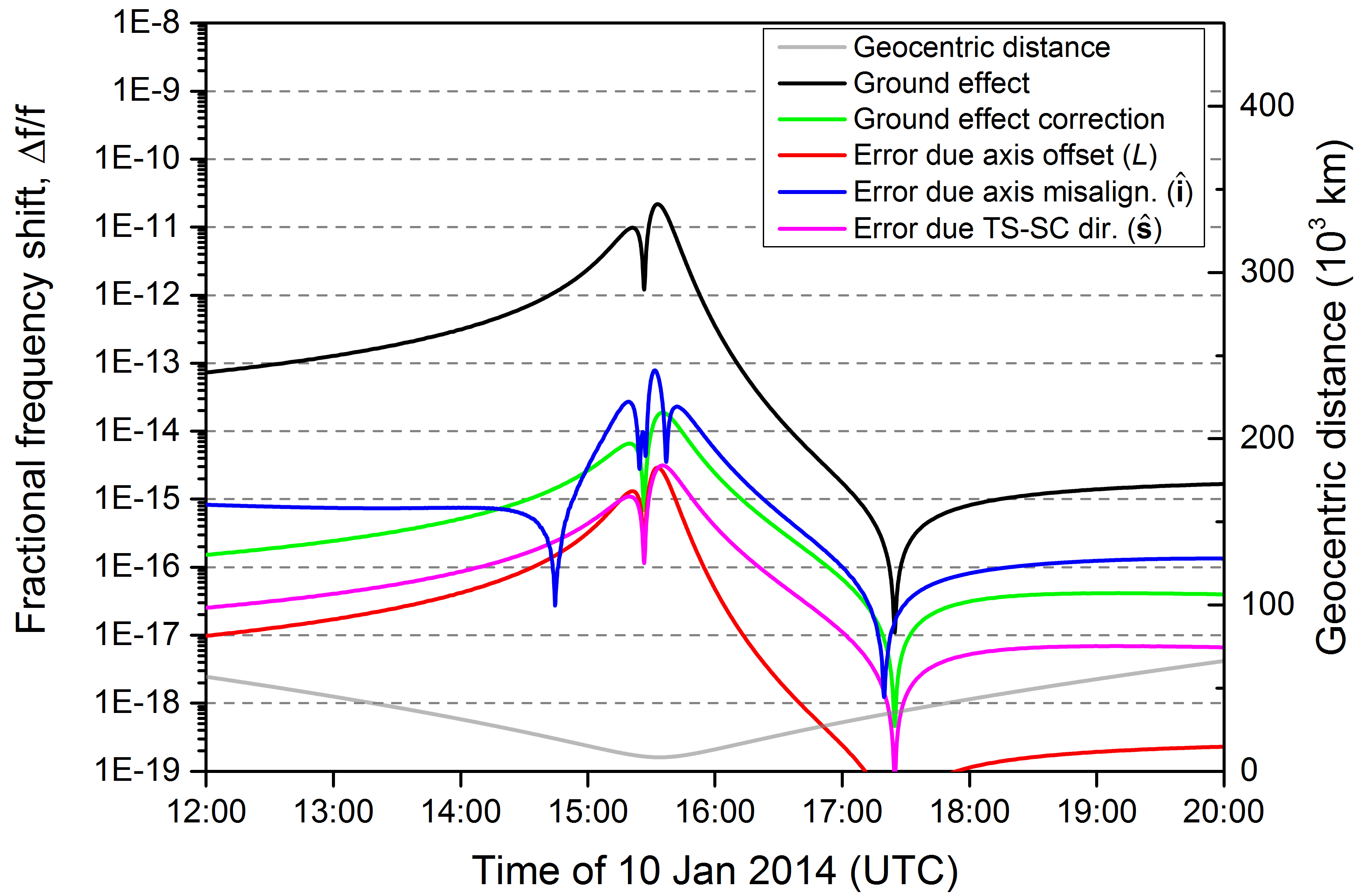
(b)

Figure 7: The APCM effect and its estimation errors for the Green Bank ground antenna tracking the RadioAstron spacecraft during low-perigee epoch A: (a) 9–23 January 2014; (b) zoom-in into the perigee of 10 January 2014. The APCM effect, denoted “ground effect” in the legend, is computed using Eq. (20). The “ground effect correction” is the error one makes in estimating the APCM effect if one uses the unprimed analogue of Eq. (20), i.e. one uses the actual antenna pointing angle $\theta$ (declination for the Green Bank NRAO140 antenna) instead of the pointing angle $\theta^{\prime}$ that corresponds to the true position of the SC. The three error curves depict the uncertainties in the computed values of the APCM effect due to the three error curves of Table 2 that are relevant to the ground APCM effect: the uncertainty in the offset between the ground antenna axes ($L$), the ground antenna axis misalignment ($\hat{\mathbf{i}}$), and the uncertainty in the TS-to-SC direction due to the SC position uncertainty ($\hat{\mathbf{s}}$). The SC visibility and ground antenna tracking constraints are not taken into account for the sake of visual clarity.

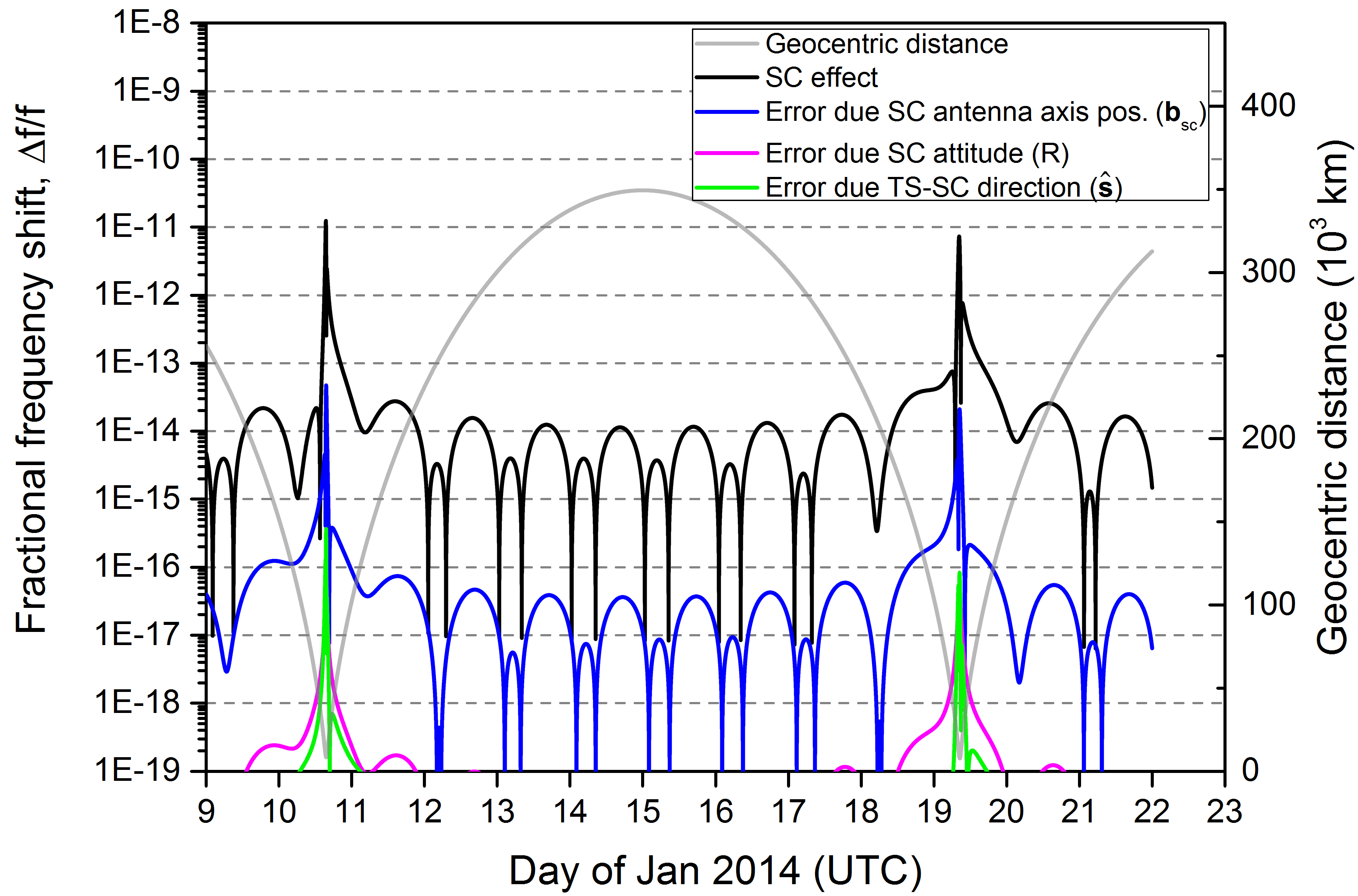
(a)

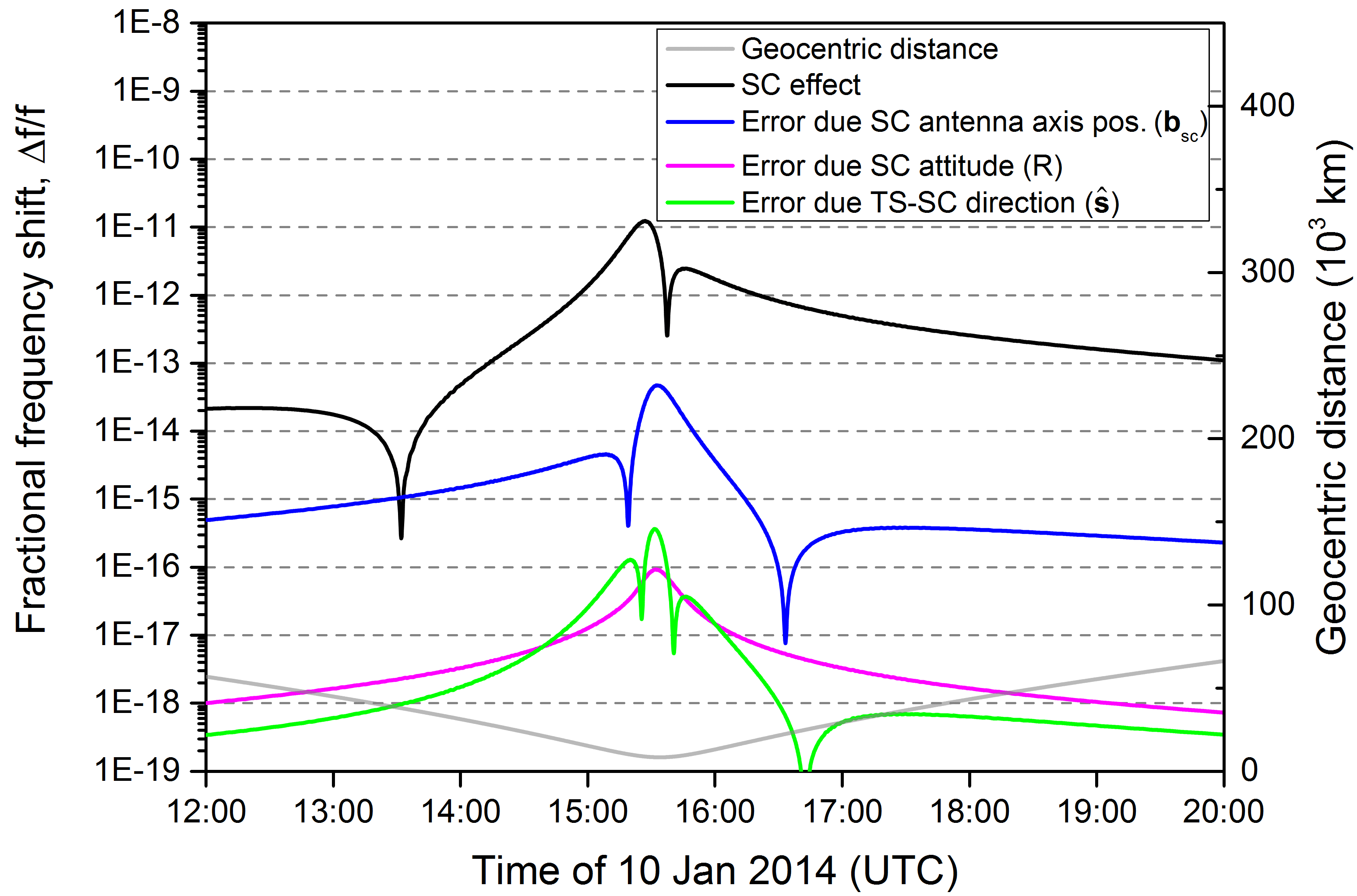
(b)

Figure 8: The APCM effect and its estimation errors for the RadioAstron on-board antenna tracking the Green Bank station during low-perigee epoch A: (a) 9–23 January 2014; (b) zoom-in into the perigee of 10 January 2014. The “SC effect” is computed using Eq. (29) with $\mathrm{R}=1$. The three error curves depict the uncertainties in the computed values of the APCM effect due to the three error sources of Table 2 that are relevant to the SC antenna: the uncertainty in the position of the intersection point of the SC antenna axes relative to the SC center of mass ($\mathbf{b}_{\mathrm{sc}}$), the uncertainty in the SC attitude ($\mathrm{R}$), and the uncertainty in the TS-to-SC direction due to the SC position uncertainty ($\hat{\mathbf{s}}$). Note that while here we assume that the SC maintains a specific constant orientation in the inertial reference frame, such that the rotation matrix $\mathrm{R}=1$, we allow for an error in the realization of this orientation by the attitude control system, $\delta\mathrm{R}\neq 0$. The SC visibility and ground antenna tracking constraints are not taken into account for the sake of visual clarity.

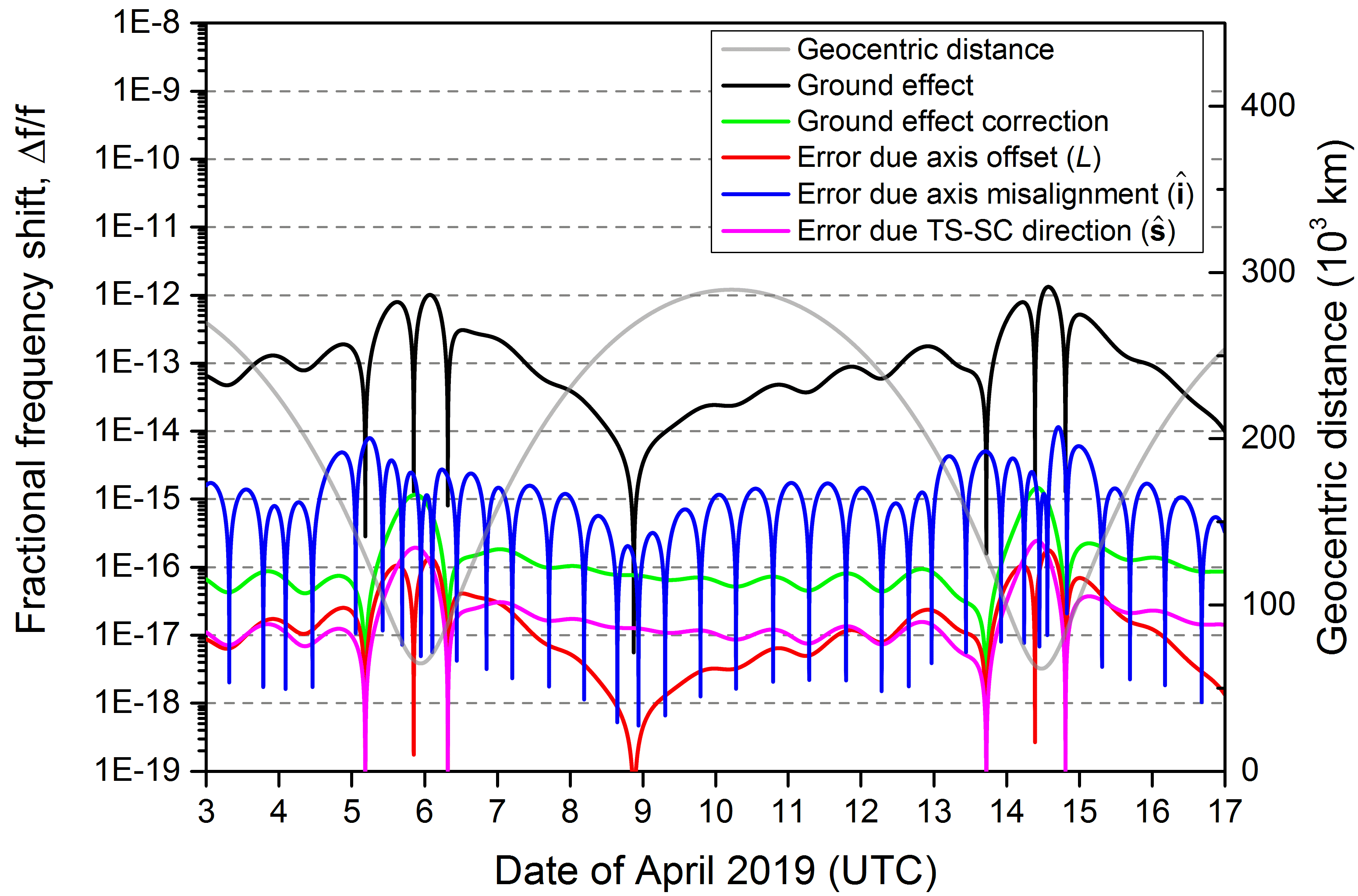
(a)

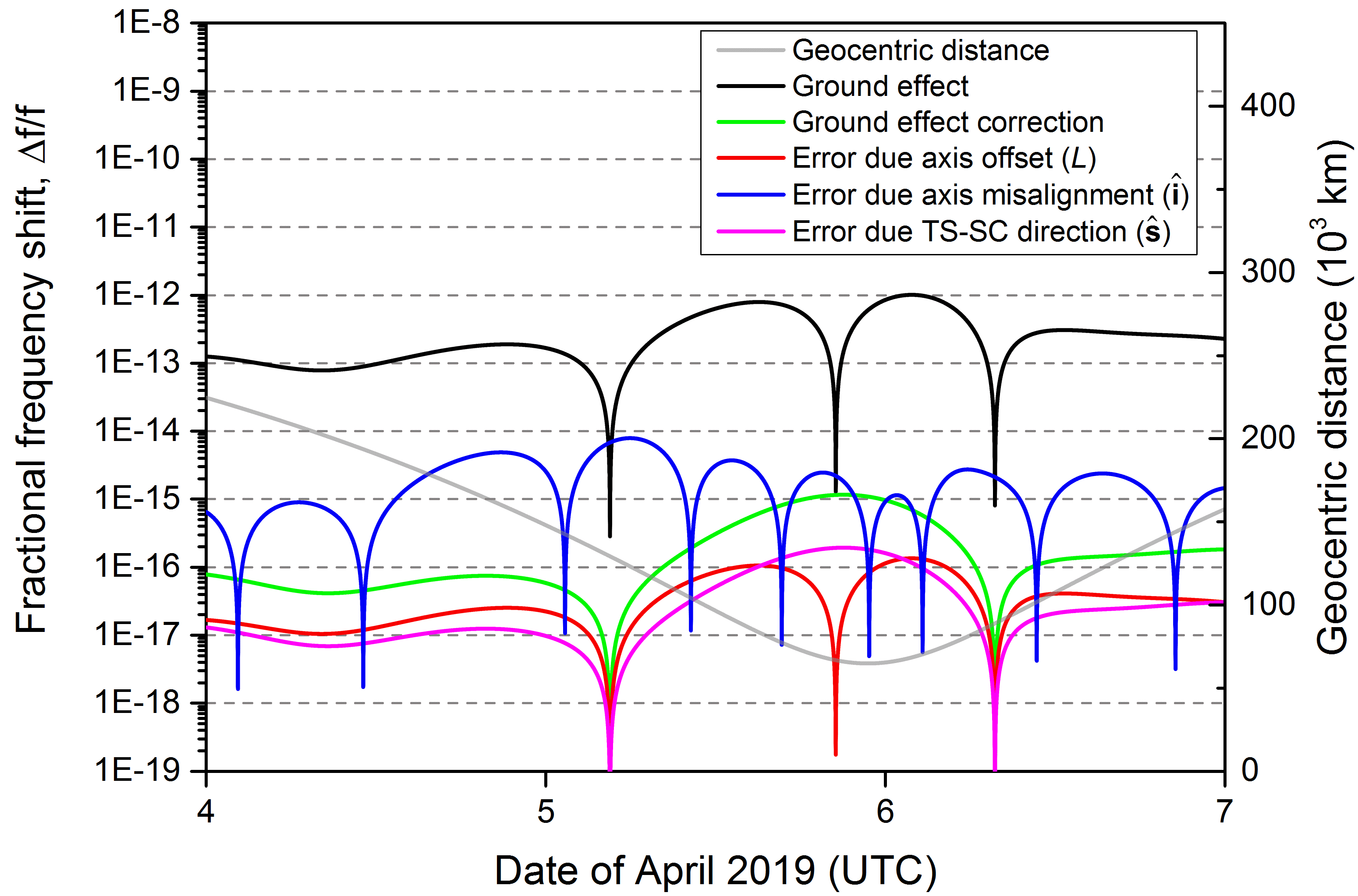
(b)

Figure 9: The APCM effect and its estimation errors for the Green Bank ground antenna tracking the RadioAstron spacecraft during high-perigee epoch B: (a) 3–17 April 2019; (b) zoom-in into the perigee of 5 April 2019. See caption of Fig. 7 for a description of the plots and other details.

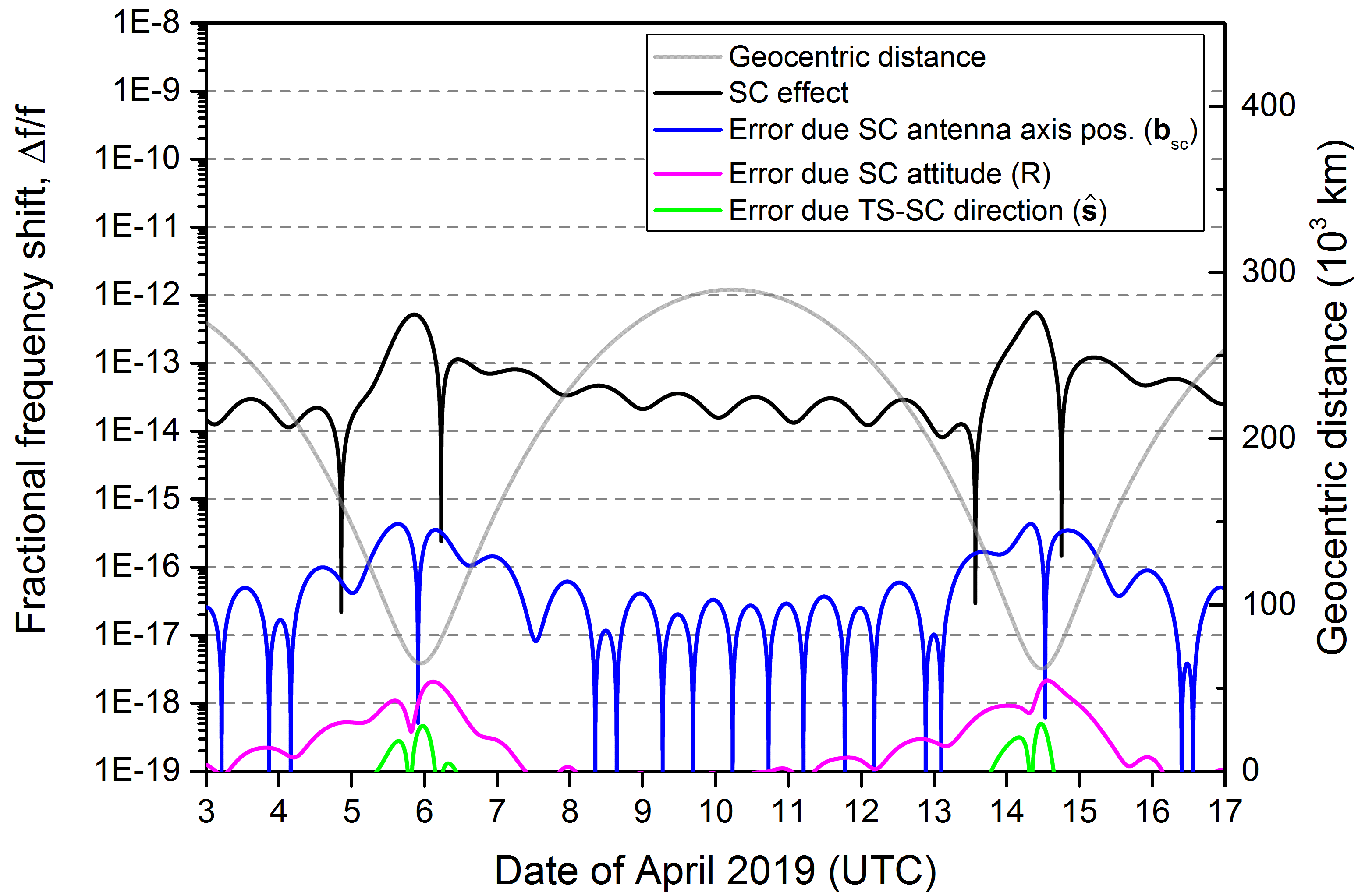
(a)

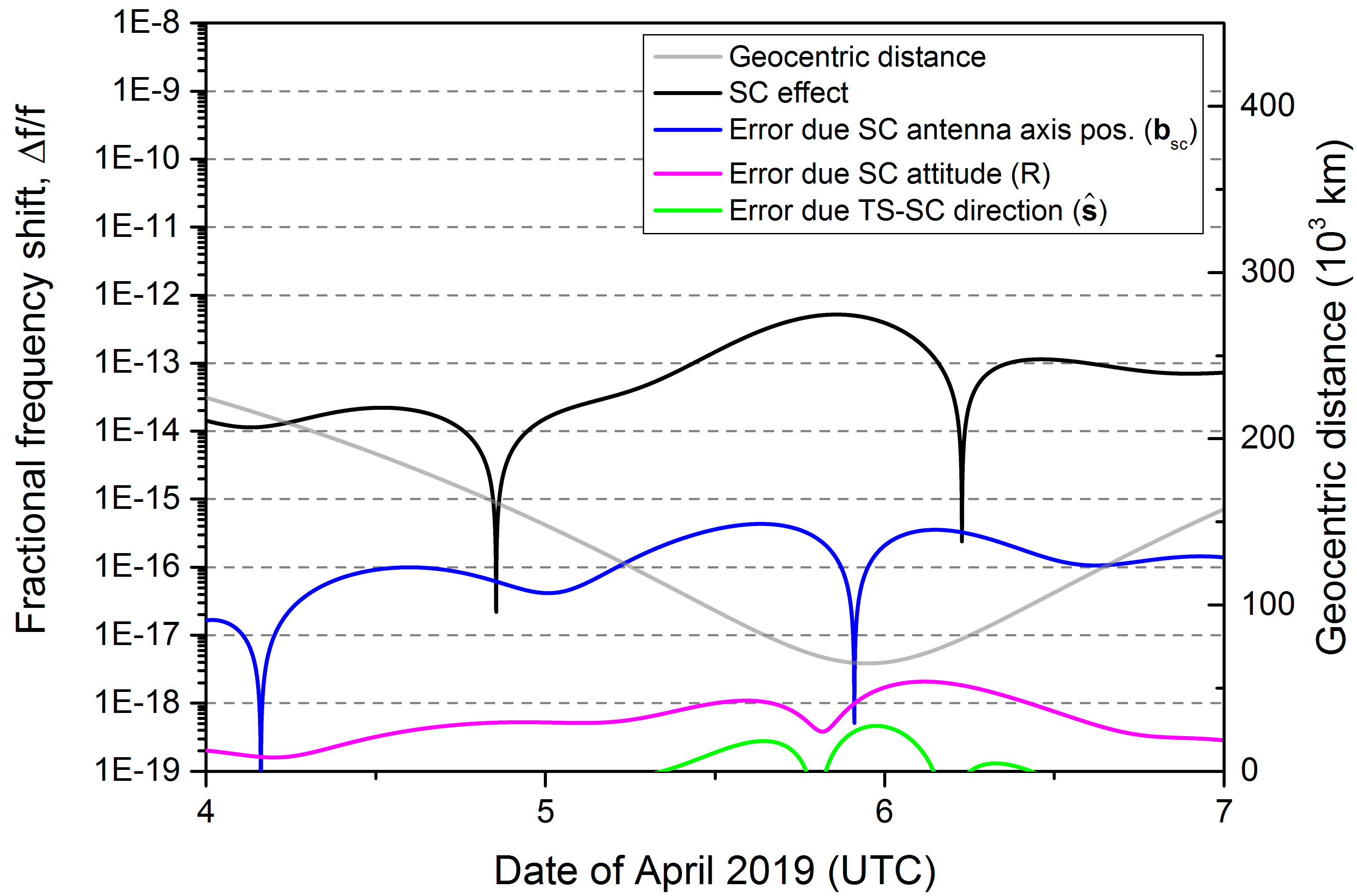
(b)

Figure 10: The APCM effect and its estimation errors for the RadioAstron on-board antenna tracking the Green Bank station during high-perigee epoch B: (a) 3–17 April 2019; (b) zoom-in into the perigee of 5 April 2019. See caption of Fig. 8 for a description of the plots and other details.

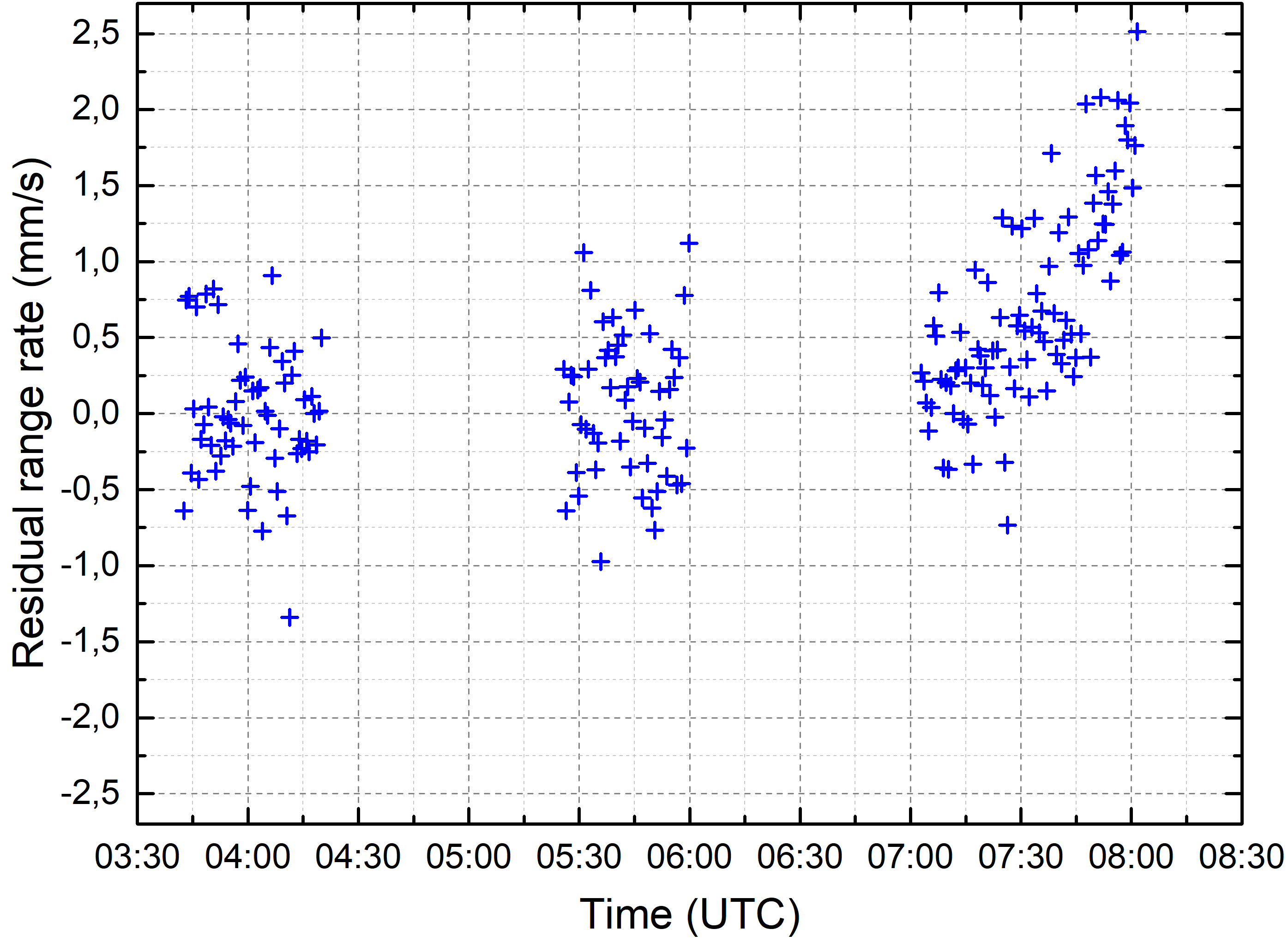
(a)

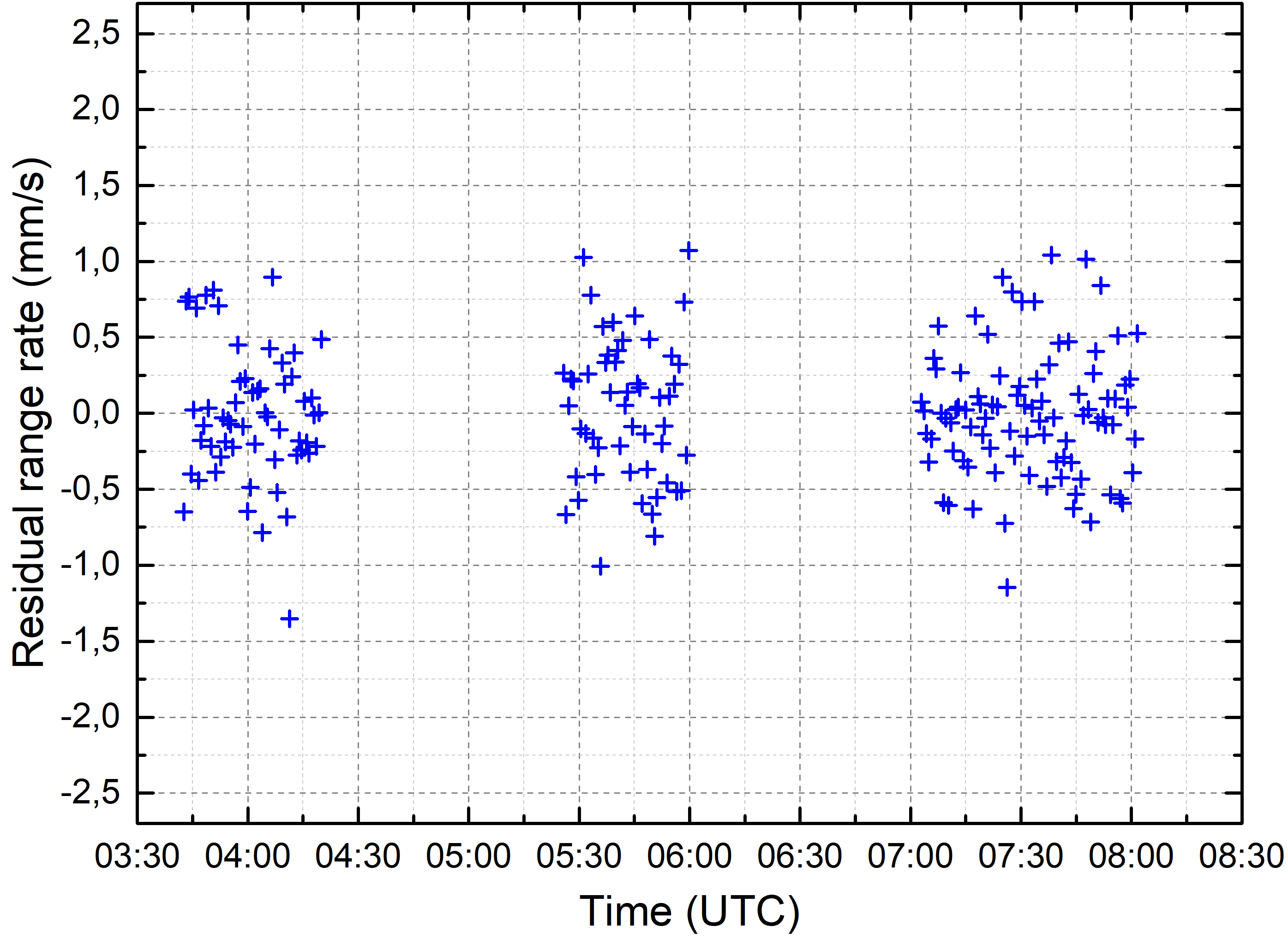
(b)

Figure 11: One-way Doppler residuals for the Green Bank antenna tracking the RadioAstron spacecraft on 19 January 2014. The APCM effects for the ground and space antennas are: (a) not taken into account; (b) taken into account. In this case the dominant contribution to the APCM effect is due to the space antenna.

Near the perigees of epoch $A$ the magnitude of the fractional frequency shift due to the APCM effect reaches $\sim 10^{-11}$ both for the ground and space antennas, which is equivalent to 3 mm/s in terms of the required velocity correction. This is significant not only for high-accuracy experiments but also for the SC orbit determination. To demonstrate this we asked the ballistic center of the KIAM to generate two orbital solutions that include the data of near-perigee observations of 19/01/2014 03:50–08:00 UTC (experiment code raks04c) performed with the Green Bank TS: one with the APCM effects not included in the model and the other taking them into account. The frequency residuals of the 8.4 GHz downlink signal, i.e. the differences between the observed frequency measurements and their computed values, that correspond to these two solutions are presented in Fig. 11. As expected, the inclusion of the APCM effects into the model results in a significantly better fit to the observational data.

4 Future missions

The technique of SVLBI, pioneered by VSOP (Hirabayashi et al., 1998) and RadioAstron, proved to be a very useful tool for radio astronomy. Several possibilities for follow-up missions are now being discussed (Gurvits, 2020). Most of them share similar features with RadioAstron: a highly eccentric orbit, a highly stable on-board frequency standard, and a large mechanically steerable high-gain antenna (see Section 1). This suggests that the results we obtained for RadioAstron will be useful in the preparation of the next generation of SVLBI missions. However, since the orbits considered for future missions are usually more circular than that of RadioAstron it seems reasonable to verify if the results presented in Section 3 are general and not peculiar to RadioAstron.

In order to address this question we repeated the computations of the previous Section for a SC with the orbital parameters specified in Table 5. These parameters are similar to those of the mission concept outlined in (Hong et al., 2014). Compared to RadioAstron, the orbit of this SC is more circular, not evolving, and has a shorter period. For our simulations we used the same ground antenna, the Green Bank Earth Station’s NRAO140 (Table 3), with the assumption of the same values for the relevant uncertainties (Table 2). For the SC we used the same values for the components of vector $\mathbf{b}$ as in Eq. (32) but assumed a 5-fold decrease in their uncertainties. We also assumed a 10-fold improvement in the accuracies of the spacecraft attitude and the TS-to-SC direction. All these assumptions are tentative and based on our analysis of the current state of the technology in the respective areas. The 10-fold improvement of the OD accuracy, which determines the uncertainty in the TS-to-SC direction, might be considered too conservative in view of the availability of high-accuracy satellite tracking means provided by satellite laser ranging and onboard GNSS receivers. However, both of these technologies currently have limited capabilities to support satellites on high Earth orbits (Winternitz et al., 2017).

Perigee (km)	10,000 km
Apogee (km)	57,131 km
Period (hr)	17.0 hr
Eccentricity	0.7
Inclination	28.5∘
RA of asc. node	220.0∘
Mean anomaly at epoch	0.0∘
Argument of perigee	0.0∘
Epoch	01/01/2030 00:00:00 UTC

Table 5: Orbital parameters assumed for the spacecraft of a possible future SVLBI mission.

The results of our simulations, spanning an arbitrarily chosen decade of 1–10 January 2030, are shown in Figs. 12 and 13. The magnitude of the APCM effect for the ground and space antennas is comparable to that of RadioAstron. The correction to the ground effect implied by Eq. (20) decreased according to our assumption of the better OD accuracy. Other errors also decreased according to our assumptions on improvements of the uncertainties. However, the error in the space APCM effect due to the uncertainty in vector $\mathbf{b}$ is still unacceptably large for high-accuracy experiments, $\sim 5\times 10^{-15}$, as well as the error in the ground APCM effect due to the ground antenna axis misalignment, $\sim 3\times 10^{-15}$.

To summarize, in this case, as with RadioAstron, the APCM effect is large enough so that it needs to be taken into account even for regular OD. The errors in its estimated values are negligible for regular OD but too large for the tracking data obtained with such antennas to be usable in experiments with modern frequency standards with frequency instability of $\sim 10^{-15}$ or better.

5 Compensation of the APCM effect

In Sections 3 and 4 we showed that the APCM effect and the errors of estimating it can be significant in spacecraft Doppler tracking experiments that demand frequency measurements with stability of better than $\sim 10^{-14}$. Now, we consider an approach to considerably reduce the magnitude of the APCM effect that is available when the SC communicates with the TS in one- and two-way modes simultaneously. All the equations derived in Section 2 are relevant to the one-way mode, i.e. when the SC transmits a signal synchronized to its on-board frequency standard and the TS receives it. In the two-way, or phase-locked loop mode, the phase of the spacecraft’s downlink signal is synchronized to that of the uplink signal   transmitted   by   the   TS.   In   order   to   obtain   the   equation

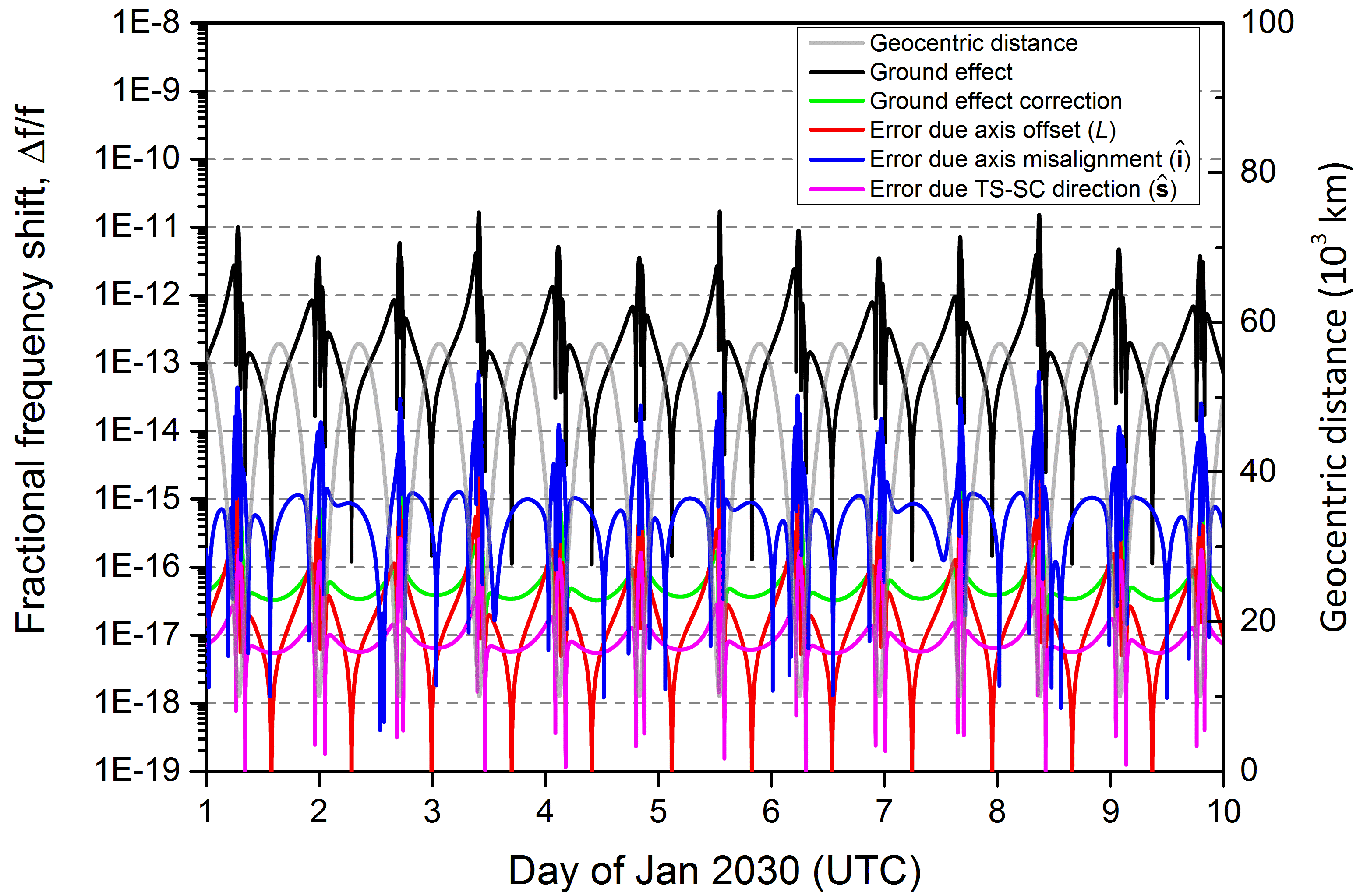
(a)

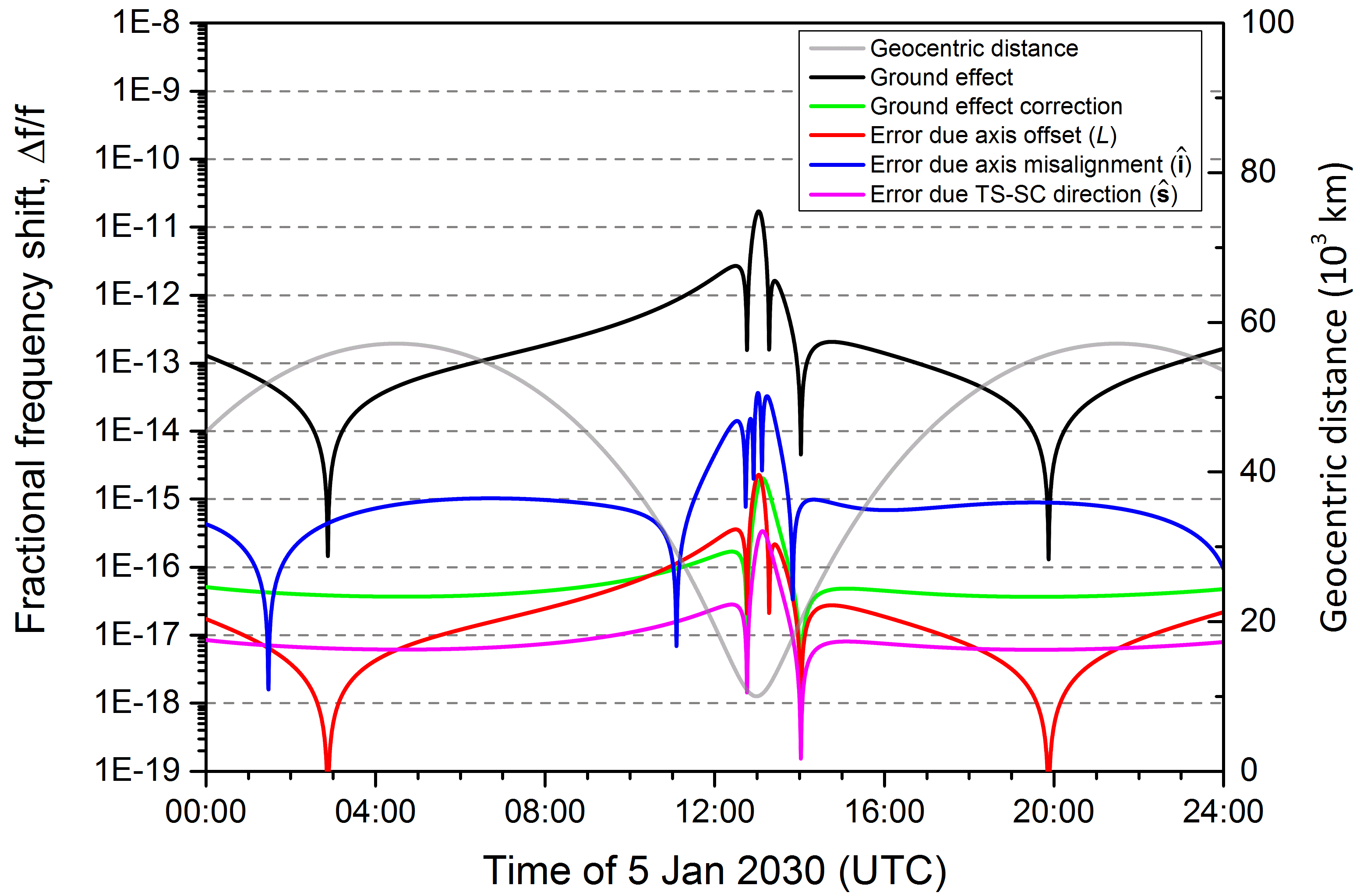
(b)

Figure 12: The APCM effect and its estimation errors for the Green Bank ground antenna tracking the spacecraft of a possible future SVLBI mission: (a) 1–10 January 2030; (b) zoom-in into the perigee of 5 January 2030. See caption of Fig. 7 for a description of the plots and other details.

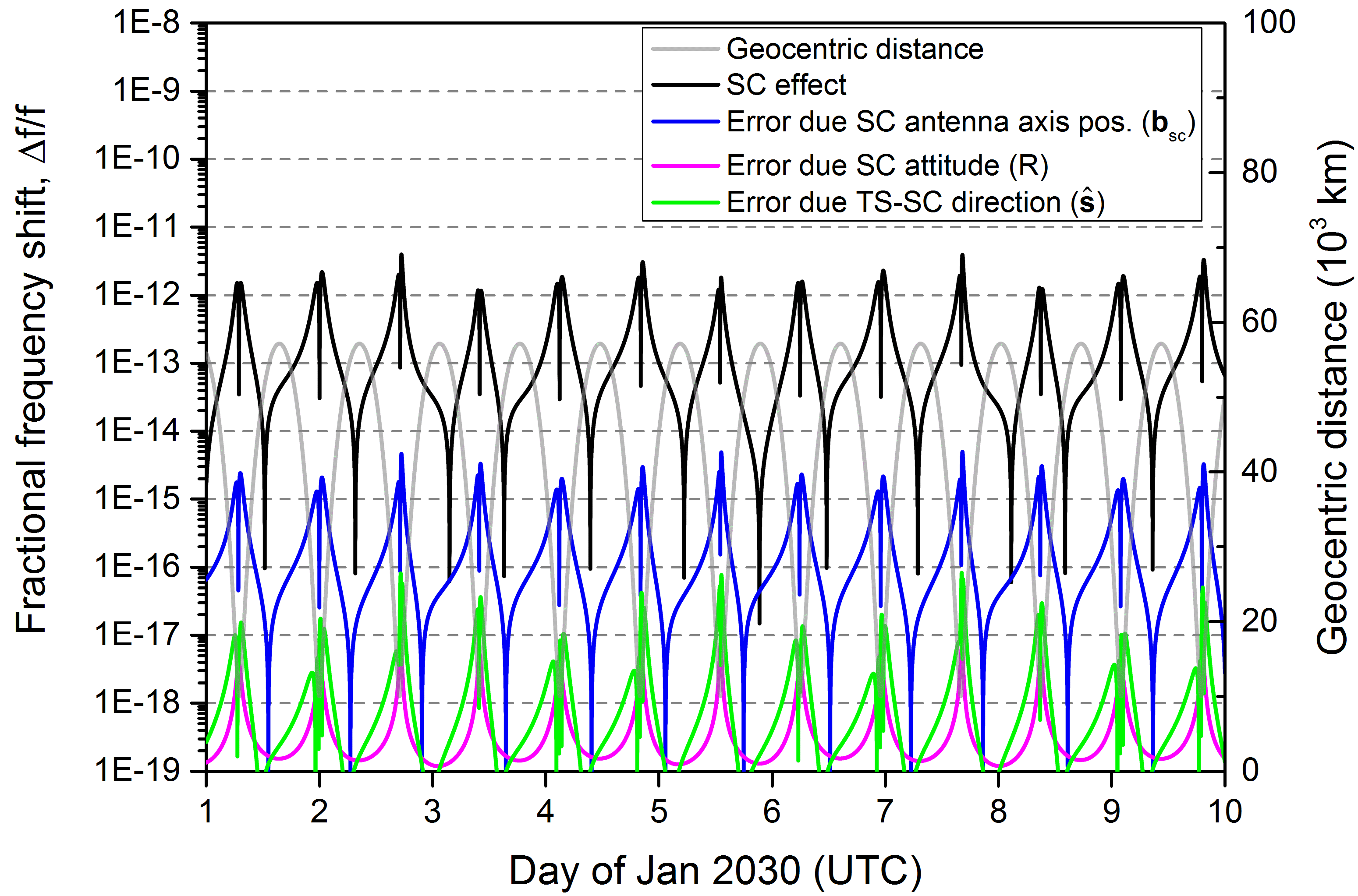
(a)

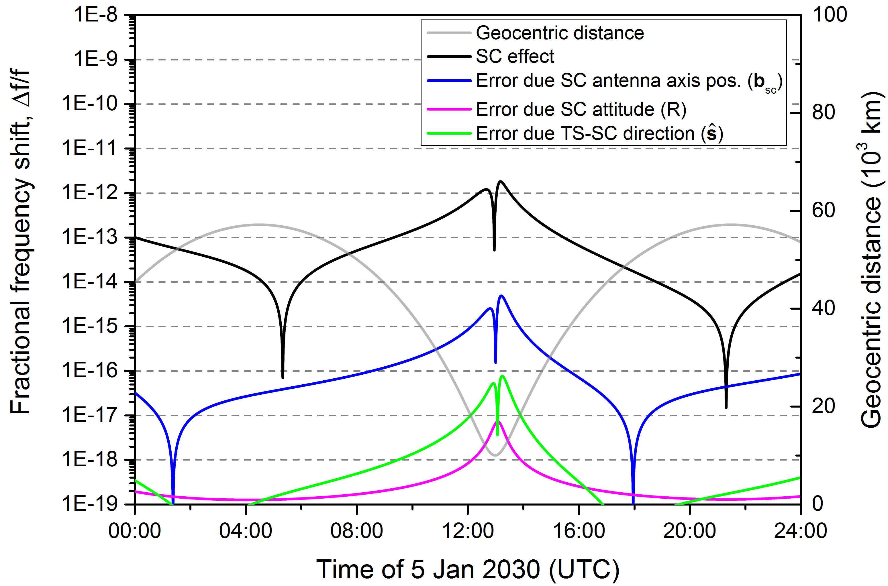
(b)

Figure 13: The APCM effect and its estimation errors for the on-board antenna of the spacecraft of a possible future SVLBI mission tracking the Green Bank station: (a) 1–10 January 2030; (b) zoom-in into the perigee of 5 January 2030. See caption of Fig. 8 for a description of the plots and other details.

for the APCM effect in this mode, we need to sum the relevant expressions for the up and down legs, taking into account the finite signal propagation time and a slight change of its propagation direction in the down leg due to the TS motion:

$$\begin{split}\frac{\Delta f_{\mathrm{2w}}^{\mathrm{(pcm)}}}{f}=\pm\frac{L}{c}\left(\sin{\theta^{\prime}_{12}}(t_{1})\cdot\dot{\theta}^{\prime}_{12}(t_{1})+\sin{\theta^{\prime}_{32}}(t_{3})\cdot\dot{\theta}^{\prime}_{32}(t_{3})\right)\\ +\>\frac{\mathbf{b^{\prime}}\cdot\mathbf{\dot{\hat{s}}}^{\prime}_{12}(t_{1})}{c}+\>\frac{\mathbf{b^{\prime}}\cdot\mathbf{\dot{\hat{s}}}^{\prime}_{32}(t_{3})}{c}+O(\delta\mathbf{\theta}^{2})+O(\delta\mathbf{s}^{2}).\end{split}$$ (33)

Here, $t_{1}$, $t_{2}$ and $t_{3}$ are the moments, respectively, when the signal is transmitted by the TS, received and retransmitted by the SC, and received by the TS (Fig. 14). Unit vector $\mathbf{\hat{s}}^{\prime}_{12}(t_{1})$ points in the direction of the signal propagation in the up leg, $\mathbf{\hat{s}}^{\prime}_{32}(t_{2})$ points in the direction opposite to that of the signal propagation in the down leg. The two ground antenna pointing angles, $\theta^{\prime}$, are defined as:

$$\theta^{\prime}_{12}(t_{1})=\frac{\pi}{2}-\angle(\mathbf{\hat{s}}^{\prime}_{12}(t_{1}),\mathbf{\hat{i}}(t_{1})),$$ (34)

$$\theta^{\prime}_{32}(t_{3})=\frac{\pi}{2}-\angle(\mathbf{\hat{s}}^{\prime}_{32}(t_{3}),\mathbf{\hat{i}}(t_{3})).$$ (35)

The other designations were introduced in Section 2. Note that in Eq. (33) the SC terms enter with the positive sign since the direction of the signal propagation in both legs is chosen op- posite to that assumed in Eqs. (27) and (28). Also note that we

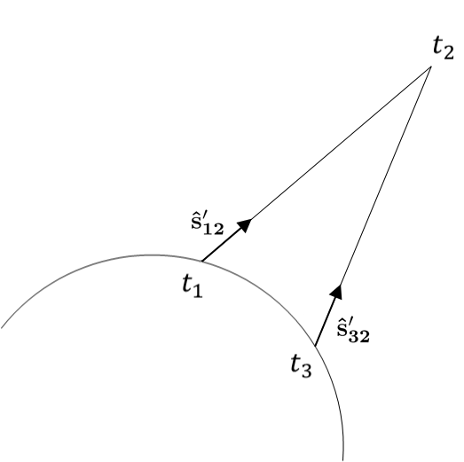
Figure 14: The schematic of the two-way signal propagation as viewed in an Earth-centered inertial reference frame. The signal is emitted by the tracking station at time $t_{1}$, received and coherently retransmitted by the spacecraft at time $t_{2}$ (neglecting the delays in the on-board equipment), and finally received by the tracking station at time $t_{3}$. During the signal travel time the tracking station slightly changes its position in the specified frame. Vector $\hat{\mathbf{s}}^{\prime}_{12}(t_{1})$ points in the direction along the signal propagation in the up leg, vector $\hat{\mathbf{s}}^{\prime}_{32}(t_{3})$ points in the direction opposite to that of the signal propagation in the down leg. The atmospheric refraction is ignored.

cannot drop the subscripts at $\theta^{\prime}$ since, for example, $\theta^{\prime}_{12}(t_{3})$ and $\theta^{\prime}_{32}(t_{3})$ are different antenna pointing angles that correspond to the SC positions, respectively, in the future and past of $t_{3}$.

Several assumptions were made in obtaining Eq. (33). The first is that the pointing errors are small, which is the basis of our analysis. Second, the signal delay in the on-board hardware was treated as negligible (actually it can be of order of a $\mu$s). We also assumed that the base frequencies of the signals in the up and down legs, $f$, are the same. In reality these frequencies are usually chosen to be different to avoid self-excitation of the antenna (for RadioAstron they are 7.2 GHz for the uplink and 8.4 and 15 GHz for the downlinks). Both of the latter aspects can be taken into account and do not change our final conclusions. Finally, we ignored the signal propagation path bending due to atmospheric refraction. This bending can be significant for low elevation angles of the ground antenna, e.g. $\delta\theta\sim 0.1^{\circ}$ for an elevation angle of 6^∘ (Sovers et al., 1998). However, since the up- and downlink signals are bent by almost exactly the same amount, $\delta\theta_{12}=\delta\theta_{32}$, the refractive corrections to the ground antenna pointing angles, $\theta^{\prime}_{12}$ and $\theta^{\prime}_{32}$, which could be introduced in Eq. (33) and Eq. (36) below, would cancel out in the final result of this Section given by Eq. (42).

If, in addition to retransmitting the signal received from the ground station, the SC also transmits a one-way signal synchronized to its on-board frequency standard, then for the frequency shift of this signal received at the TS at a time $t_{3}$ we have:

$$\begin{split}\frac{\Delta f_{\mathrm{1w}}^{\mathrm{(pcm)}}}{f}=\pm\frac{L}{c}\sin{\theta^{\prime}_{32}}(t_{3})\cdot\dot{\theta}^{\prime}_{32}(t_{3})+\frac{\mathbf{b^{\prime}}\cdot\dot{\hat{\mathbf{s}}}^{\prime}_{32}(t_{3})}{c}\\ +O(\delta\mathbf{\theta}^{2})+O(\delta\mathbf{s}^{2}).\end{split}$$ (36)

Again, this signal is usually transmitted at a frequency different from those of the up and down legs of the two-way signal, but we ignore it here.

The total frequency shift experienced by the one-way signal is a sum of contributions of various factors:

$$\Delta f_{\mathrm{1w}}=\Delta f_{\mathrm{kin}}+\Delta f_{\mathrm{grav}}+\Delta f_{\mathrm{media}}+\Delta f_{\mathrm{1w}}^{\mathrm{(pcm)}}+\Delta f_{\mathrm{1w}}^{\mathrm{(other)}},$$ (37)

where $\Delta f_{\mathrm{kin}}$ is the kinematic frequency shift of the first order in $v/c$, $\Delta f_{\mathrm{grav}}$ is the gravitational redshift, $\Delta f_{\mathrm{media}}$ is the correction due to the propagation media, $\Delta f_{\mathrm{1w}}^{\mathrm{(pcm)}}$ is the correction due to the APCM effect given by Eq. (36), and $\Delta f_{\mathrm{1w}}^{\mathrm{(other)}}$ is the contribution of other factors such as higher-order kinematic terms, instrumental effects, etc. Similarly, for the two-way signal we have:

$$\begin{split}\Delta f_{\mathrm{2w}}=2\Delta f_{\mathrm{kin}}+2\Delta f_{\mathrm{media}}+\Delta f_{\mathrm{2w}}^{\mathrm{(pcm)}}+\Delta f_{\mathrm{2w}}^{\mathrm{(other)}}+\Delta f^{\mathrm{(res)}},\end{split}$$ (38)

where $\Delta f_{\mathrm{2w}}^{\mathrm{(pcm)}}$ is the correction due to the APCM effect given by Eq. (33) and $\Delta f_{\mathrm{2w}}^{\mathrm{(other)}}$ labels the contribution of the “other” terms (see above) relevant to the two-way mode. Note that the two-way signal does not experience the gravitational frequency shift and, up to residual terms grouped into $\Delta f^{\mathrm{(res)}}$, has twice the kinematic and media contributions compared to the one-way signal. These residual terms are due to variations of the media properties on the time scale of signal propagation and the spatial scale of non-reciprocity of the signal paths of the up and down legs. Usually these terms are smaller than the respective contributions of $\Delta f_{\mathrm{kin}}$ and $\Delta f_{\mathrm{media}}$ by several orders of magnitude (Vessot & Levine, 1979; Litvinov et al., 2018).

Now, let us consider the following combination of the one- and two-way measurements: $\Delta f_{\mathrm{1w}}-\dfrac{\Delta f_{\mathrm{2w}}}{2}$. Using Eqs. (37) and (38) we obtain:

$$\Delta f_{\mathrm{1w}}-\frac{\Delta f_{\mathrm{2w}}}{2}=\Delta f_{\mathrm{grav}}+\Delta f_{\mathrm{kin}}^{\mathrm{(res)}}+\Delta f_{\mathrm{media}}^{\mathrm{(res)}}+\Delta f_{\mathrm{pcm}}^{\mathrm{(res)}}+\Delta f_{\mathrm{other}}^{\mathrm{(res)}}.$$ (39)

Here we split the residual terms of Eq. (38) into its kinematic, media, and “other” components and denoted

$$\Delta f_{\mathrm{pcm}}^{\mathrm{(res)}}=\Delta f_{\mathrm{1w}}^{\mathrm{(pcm)}}-\frac{\Delta f_{\mathrm{2w}}^{\mathrm{(pcm)}}}{2}.$$ (40)

A notable feature of Eq. (39) is that its right-hand side fully retains the contribution of the gravitational frequency shift of the one-way downlink signal, $\Delta f_{\mathrm{grav}}$, but the dominant contributions of the nonrelativistic Doppler shift and the troposphere

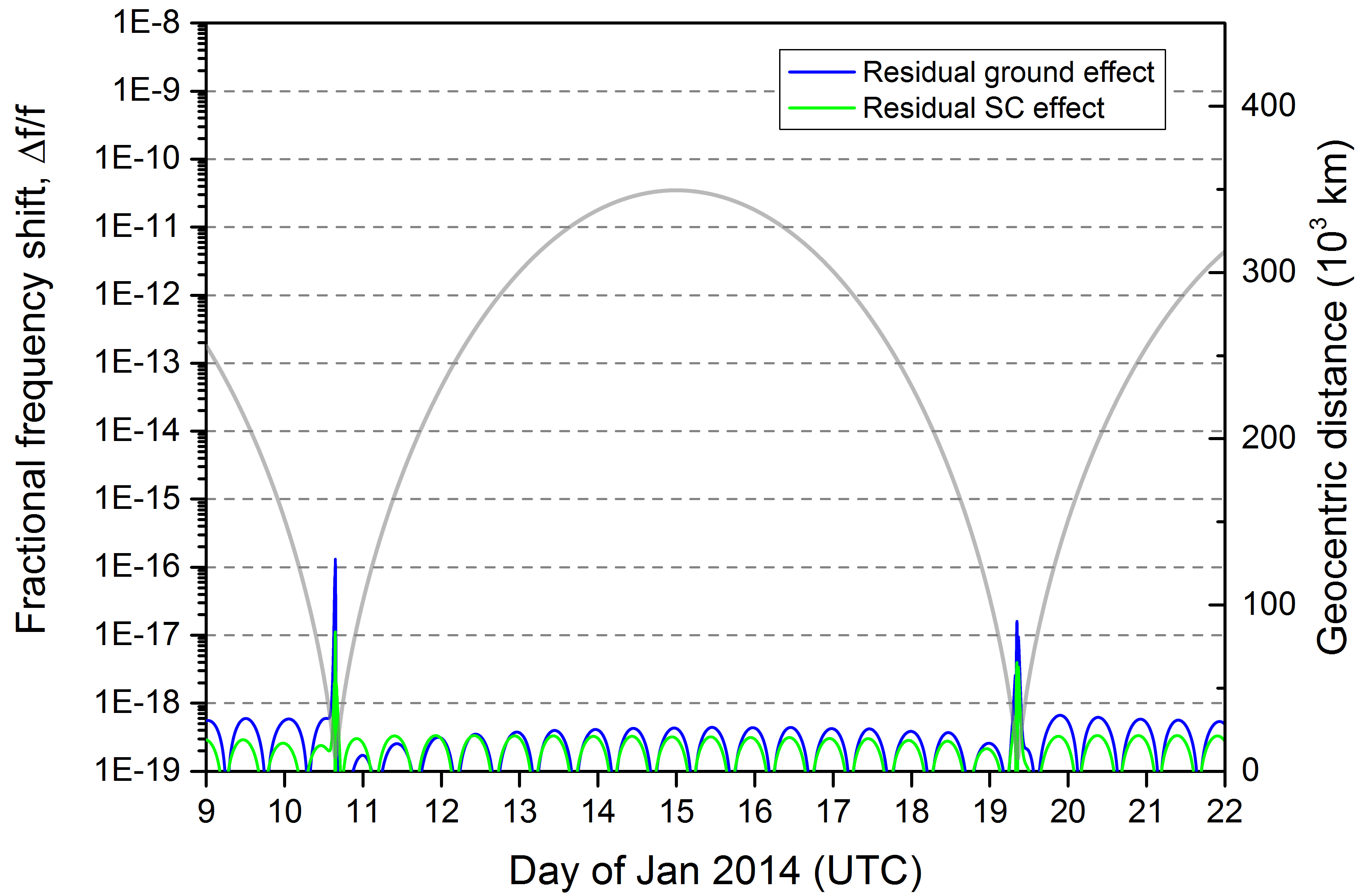
(a)

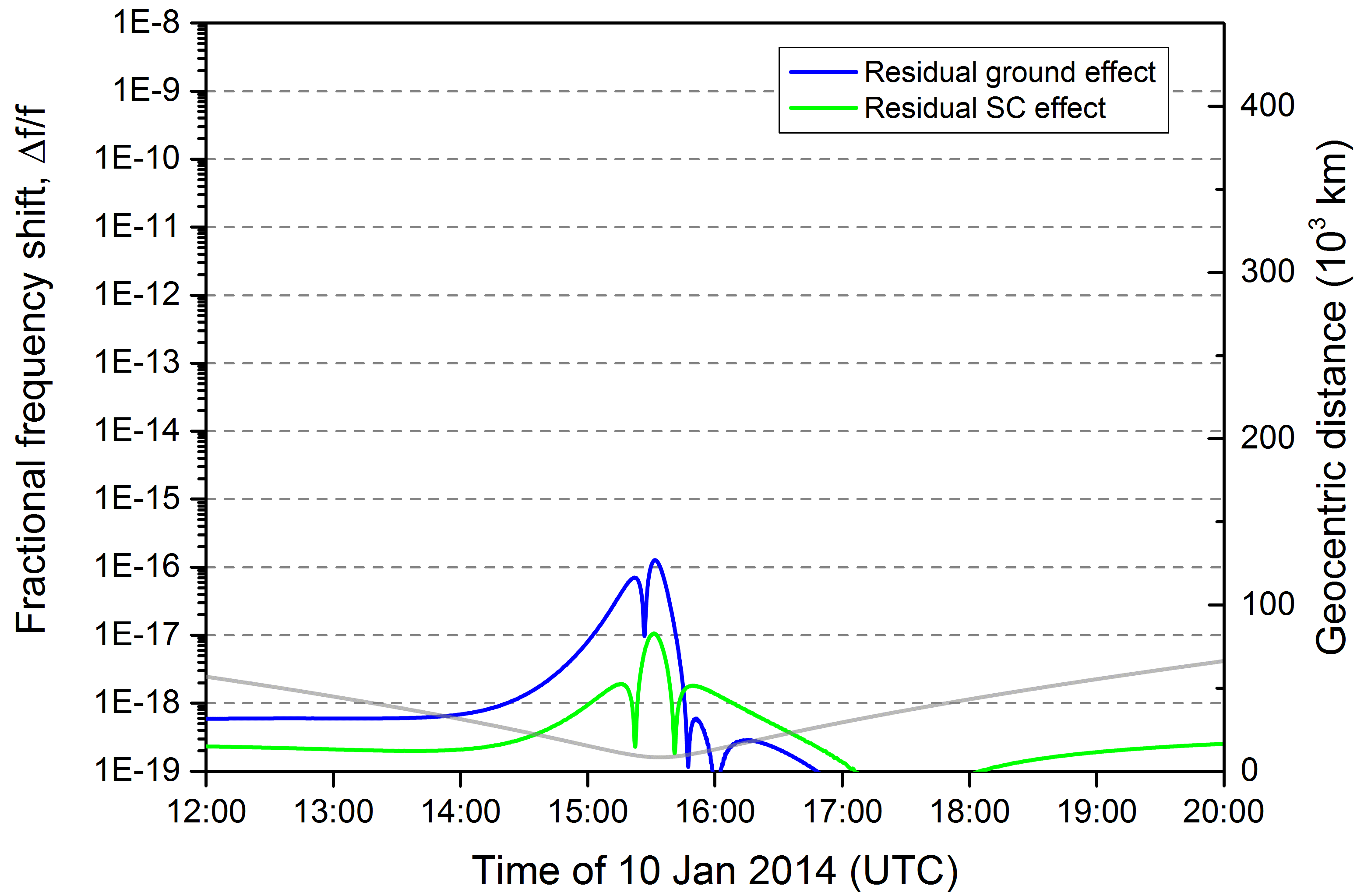
(b)

Figure 15: The residual APCM effect for the on-board and ground antennas after application of the compensation scheme of Eq. (39). The Green Bank station antenna tracking the RadioAstron spacecraft: (a) 9–23 January 2014; (b) zoom-in into the perigee of 10 January 2014.

are cancelled or, at minimum, reduced by many orders of magnitude, down to their residual terms labelled $\Delta f_{\mathrm{kin}}^{\mathrm{(res)}}$ and $\Delta f_{\mathrm{media}}^{\mathrm{(res)}}$.

The importance of Eq. (39) for high-accuracy gravity-related experiments was first recognized in the Gravity Probe A mission that measured the gravitational redshift, and the relevant violation parameter of the Einstein Equivalence Principle, with an accuracy of about 0.01% (Vessot et al., 1980). The space probe of that mission, however, used a low-gain non-tracking antenna and the APCM effect was not considered. An approach based on Eq. (39) is also used in the gravitational redshift experiment with RadioAstron (Litvinov et al., 2018; Nunes et al., 2020) and now makes an integral part of almost every prospective mission to measure the gravitational redshift (Altschul et al., 2015).

Our goal is to demonstrate that the residual APCM effect term in Eq. (39), $\Delta f_{\mathrm{pcm}}^{(\mathrm{res})}$, is significantly reduced compared to $\Delta f_{\mathrm{1w}}^{\mathrm{(pcm)}}$ and $\Delta f_{\mathrm{2w}}^{\mathrm{(pcm)}}$, similar to the reduction of the nonrelativistic Doppler and tropospheric terms. For simplicity let us consider the case of a polar mount ground antenna, so that the vector $\hat{\mathbf{i}}$ along its primary axis does not depend on time in an Earth-centered inertial reference frame (the change of $\hat{\mathbf{i}}$ due to the Earth’s nutation and polar motion can be neglected on the time scale of signal propagation). Then, using Eqs. (36) and  (33), as well as the expansion of

$$\begin{split}\mathbf{\hat{s}}^{\prime}_{12}(t_{1})=\;&\mathbf{\hat{s}}^{\prime}_{32}(t_{3})+2\frac{\mathbf{v}_{\mathrm{e}}(t_{3})}{c}\\ &-2\left(\frac{\mathbf{v}_{\mathrm{e}}(t_{3})}{c}\cdot\mathbf{\hat{s}}^{\prime}_{32}(t_{3})\right)\mathbf{\hat{s}}^{\prime}_{32}(t_{3})+O\left(\frac{v_{\mathrm{e}}}{c}\right)^{2},\end{split}$$ (41)

which straightforwardly follows from the relation between successive positions of the TS and its velocity, $\mathbf{v}_{\mathrm{e}}$, in a chosen Earth-centered inertial reference frame, we obtain:

$$\begin{split}\frac{\Delta f_{\mathrm{pcm}}^{\mathrm{(res)}}}{f}=\mp\frac{L}{c^{2}}\bigg{\{}\frac{\dot{\theta}^{\prime}}{\cos^{2}\theta^{\prime}}\left(\left(\mathbf{v}-\left(\mathbf{v}\cdot\mathbf{\hat{s}}^{\prime}\right)\mathbf{\hat{s}}^{\prime}\right)\cdot\hat{\mathbf{i}}\right)\\ +\tan\theta^{\prime}\left[\left(\left(\mathbf{a}-\left(\mathbf{a}\cdot\mathbf{\hat{s}}^{\prime}\right)\mathbf{\hat{s}}^{\prime}-\left(\mathbf{v}\cdot\dot{\hat{\mathbf{s}}}^{\prime}\right)\mathbf{\hat{s}}^{\prime}-\left(\mathbf{v}\cdot\mathbf{\hat{s}}^{\prime}\right)\dot{\hat{\mathbf{s}}}^{\prime}\right)\cdot\hat{\mathbf{i}}\right)\right]\bigg{\}}\\ -\,\frac{1}{c^{2}}\bigg{(}\mathbf{b^{\prime}}\cdot\left(\mathbf{a}-\left(\mathbf{a}\cdot\mathbf{\hat{s}}^{\prime}\right)\mathbf{\hat{s}}^{\prime}-\left(\mathbf{v}\cdot\dot{\hat{\mathbf{s}}}^{\prime}\right)\mathbf{\hat{s}}^{\prime}-\left(\mathbf{v}\cdot\mathbf{\hat{s}}^{\prime}\right)\dot{\hat{\mathbf{s}}}^{\prime}\right)\bigg{)}\\ +O(\delta\mathbf{\theta}^{2})+O(\delta\mathbf{s}^{2})+O(v/c)^{3},\end{split}$$ (42)

where, for brevity, we labeled: $\theta^{\prime}=\theta^{\prime}_{32}(t_{3})$, $\mathbf{\hat{s}}^{\prime}=\mathbf{\hat{s}}^{\prime}_{32}(t_{3})$, $\mathbf{v}=\mathbf{v}_{\mathrm{e}}(t_{3})$, and $\mathbf{a}=\mathbf{\dot{v}}_{\mathrm{e}}(t_{3})$. Although Eq. (42) looks cumbersome, it is clearly of $O(1/c)^{2}$. Thus we expect the residual APCM effect, $\Delta f_{\mathrm{pcm}}^{\mathrm{(res)}}$, to be much smaller than those in the one-way and two-way modes since the latter are of $O(1/c)$.

To demonstrate this we use the RadioAstron SC again. RadioAstron implemented the compensation scheme described above not fully in that the one- and two-way modes could be operated only intermittently but not simultaneously. This adds complication to the actual data processing but is not significant for our illustrative purposes. The residual APCM effect for RadioAstron during the low perigee epoch of January 2014 is shown in Fig. 15 assuming simultaneous tracking in the one- and two-way modes. Comparing it to Figs. 7 and 8 we note that the peak values of the ground APCM effect are reduced by 5 orders of magnitude and those of the space APCM effect, respectively, by 6. None of the two residual effects exceeds $1.3\times 10^{-16}$. In particular, such a significant reduction makes them negligible for the RadioAstron gravitational redshift experiment. Although such residual effect may not be negligible for future high-accuracy SC tracking experiments using the next generation of frequency standards with accuracy and stability of $\sim 10^{-16}$, it will clearly be possible to take it into account accurately enough using Eq. (42).

6 Conclusions

We have improved the model for the antenna phase center motion (APCM) effect for high-gain mechanically steerable antennas by taking into account pointing errors made by the antenna while tracking the source/target. This improvement is particularly relevant for high-accuracy SC tracking experiments. Using the data from radio tracking experiments performed with the RadioAstron spacecraft we showed that the magnitude of the APCM effect can be very large for spacecraft on highly elliptic orbits, i.e. of order $10^{-11}$ in terms of the fractional frequency shift both for ground and spaceborne antennas. The fractional frequency shift due to our correction to the APCM effect model can reach $2\times 10^{-14}$ for RadioAstron.

We also found that the error of taking the APCM effect into account can be as large $4\times 10^{-14}$. This is significant for many kinds of high-accuracy experiments, e.g. those concerned with studies of gravity. The largest contribution to the error is due to the uncertainty in the position of the intersection point of the SC antenna rotation axes relative to the SC center of mass, the ground antenna axis offset and the ground antenna axis misalignment. We found that the error due to the latter can reach even higher values, up to $7\times 10^{-14}$. However, we consider this value as preliminary according to the tentative value of the NRAO140 antenna axis misalignment we used.

We also considered a possible future SVLBI mission with a SC on a less eccentric orbit compared to RadioAstron and with an improved error budget. We found that in this case both the APCM effect and its errors are still unacceptably large for high-accuracy Doppler tracking experiments.

Finally, we showed that the APCM effect can be significantly reduced by using a specific configuration of the satellite communications links, i.e. by combining the data of simultaneous one- and two-way frequency measurements. For the case of RadioAstron this reduces both the ground and space APCM effects down to below $1\times 10^{-16}$, which provides a way for using high-gain mechanically steerable antennas in high-accuracy SC tracking experiments in the near future.

References

- Altschul et al. (2015) Altschul, B., Bailey, Q. G., Blanchet, L., Bongs, K., Bouyer, P., Cacciapuoti, L., Capozziello, S., Gaaloul, N., Giulini, D., Hartwig, J., Iess, L., Jetzer, P., Landragin, A., Rasel, E., Reynaud, S., Schiller, S., Schubert, C., Sorrentino, F., Sterr, U., Tasson, J. D., Tino, G. M., Tuckey, P., & Wolf, P. (2015). Quantum tests of the Einstein Equivalence Principle with the STE-QUEST space mission. Advances in Space Research, 55, 501–524. doi:10.1016/j.asr.2014.07.014. arXiv:1404.4307.
- Biriukov et al. (2014) Biriukov, A. V., Kauts, V. L., Kulagin, V. V., Litvinov, D. A., & Rudenko, V. N. (2014). Gravitational redshift test with the space radio telescope ‘‘RadioAstron’’. Astronomy Reports, 58(11), 783--795. doi:10.1134/S1063772914110018.
- Bothwell et al. (2019) Bothwell, T., Kedar, D., Oelker, E., Robinson, J. M., Bromley, S. L., Tew, W. L., Ye, J., & Kennedy, C. J. (2019). JILA SrI optical lattice clock with uncertainty of . Metrologia, 56(6), 065004. doi:10.1088/1681-7575/ab4089. arXiv:1906.06004.
- Duev et al. (2012) Duev, D. A., Molera Calvés, G., Pogrebenko, S. V., Gurvits, L. I., Cimó, G., & Bocanegra Bahamon, T. (2012). Spacecraft VLBI and Doppler tracking: algorithms and implementation. Astronomy & Astrophysics, 541, A43. doi:10.1051/0004-6361/201218885. arXiv:1203.4408.
- Fedorchuk & Arkhipov (2014) Fedorchuk, S. D., & Arkhipov, M. Y. (2014). On the assurance of the design accuracy of the space radio telescope RadioAstron. Cosmic Research, 52, 379--381. doi:10.1134/S0010952514050049.
- Ford et al. (2014) Ford, H. A., Anderson, R., Belousov, K., Brandt, J. J., Ford, J. M., Kanevsky, B., Kovalenko, A., Kovalev, Y. Y., Maddalena, R. J., Sergeev, S., Smirnov, A., Watts, G., & Weadon, T. L. (2014). The RadioAstron Green Bank Earth Station. In L. M. Stepp, R. Gilmozzi, & H. J. Hall (Eds.), Ground-based and Airborne Telescopes V Proc. SPIE 9145 (p. 91450B). doi:10.1117/12.2056761.
- Giovannini et al. (2018) Giovannini, G., Savolainen, T., Orienti, M., Nakamura, M., Nagai, H., Kino, M., Giroletti, M., Hada, K., Bruni, G., Kovalev, Y. Y., Anderson, J. M., D’Ammando, F., Hodgson, J., Honma, M., Krichbaum, T. P., Lee, S. S., Lico, R., Lisakov, M. M., Lobanov, A. P., Petrov, L., Sohn, B. W., Sokolovsky, K. V., Voitsik, P. A., Zensus, J. A., & Tingay, S. (2018). A wide and collimated radio jet in 3C84 on the scale of a few hundred gravitational radii. Nature Astronomy, 2, 472--477. doi:10.1038/s41550-018-0431-2. arXiv:1804.02198.
- Gurvits (2020) Gurvits, L. I. (2020). Space VLBI: from first ideas to operational missions. Advances in Space Research, 65(2), 868--876. doi:10.1016/j.asr.2019.05.042. arXiv:1905.11175.
- Heß et al. (2011) Heß, M. P., Stringhetti, L., Hummelsberger, B., Hausner, K., Stalford, R., Nasca, R., Cacciapuoti, L., Much, R., Feltham, S., Vudali, T., Léger, B., Picard, F., Massonnet, D., Rochat, P., Goujon, D., Schäfer, W., Laurent, P., Lemonde, P., Clairon, A., Wolf, P., Salomon, C., Procházka, I., Schreiber, U., & Montenbruck, O. (2011). The ACES mission: System development and test status. Acta Astronautica, 69, 929--938. doi:10.1016/j.actaastro.2011.07.002.
- Hirabayashi et al. (1998) Hirabayashi, H., Hirosawa, H., Kobayashi, H., Murata, Y., Edwards, P. G., Fomalont, E. B., Fujisawa, K., Ichikawa, T., Kii, T., Lovell, J. E. J., Moellenbrock, G. A., Okayasu, R., Inoue, M., Kawaguchi, N., Kameno, S., Shibata, K. M., Asaki, Y., Bushimata, T., Enome, S., Horiuchi, S., Miyaji, T., Umemoto, T., Migenes, V., Wajima, K., Nakajima, J., Morimoto, M., Ellis, J., Meier, D. L., Murphy, D. W., Preston, R. A., Smith, J. G., Tingay, S. J., Traub, D. L., Wietfeldt, R. D., Benson, J. M., Claussen, M. J., Flatters, C., Romney, J. D., Ulvestad, J. S., D’Addario, L. R., Langston, G. I., Minter, A. H., Carlson, B. R., Dewdney, P. E., Jauncey, D. L., Reynolds, J. E., Taylor, A. R., McCulloch, P. M., Cannon, W. H., Gurvits, L. I., Mioduszewski, A. J., Schilizzi, R. T., & Booth, R. S. (1998). Overview and Initial Results of the Very Long Baseline Interferometry Space Observatory Programme. Science, 281, 1825. doi:10.1126/science.281.5384.1825.
- Hong et al. (2014) Hong, X., Shen, Z., An, T., & Liu, Q. (2014). The Chinese space Millimeter-wavelength VLBI array - A step toward imaging the most compact astronomical objects. Acta Astronautica, 102, 217--225. doi:10.1016/j.actaastro.2014.05.026. arXiv:1403.5188.
- Johnson et al. (2016) Johnson, M. D., Kovalev, Y. Y., Gwinn, C. R., Gurvits, L. I., Narayan, R., Macquart, J.-P., Jauncey, D. L., Voitsik, P. A., Anderson, J. M., Sokolovsky, K. V., & Lisakov, M. M. (2016). Extreme Brightness Temperatures and Refractive Substructure in 3C273 with RadioAstron. Astrophys. J. Letters, 820(1), L10. doi:10.3847/2041-8205/820/1/L10. arXiv:1601.05810.
- Kardashev et al. (2013) Kardashev, N. S., Khartov, V. V., Abramov, V. V., Avdeev, V. Y., Alakoz, A. V., Aleksandrov, Y. A., Ananthakrishnan, S., Andreyanov, V. V., Andrianov, A. S., Antonov, N. M., Artyukhov, M. I., Arkhipov, M. Y., Baan, W., Babakin, N. G., Babyshkin, V. E., Bartel’, N., Belousov, K. G., Belyaev, A. A., Berulis, J. J., Burke, B. F., Biryukov, A. V., Bubnov, A. E., Burgin, M. S., Busca, G., Bykadorov, A. A., Bychkova, V. S., Vasil’kov, V. I., Wellington, K. J., Vinogradov, I. S., Wietfeldt, R., Voitsik, P. A., Gvamichava, A. S., Girin, I. A., Gurvits, L. I., Dagkesamanskii, R. D., D’Addario, L., Giovannini, G., Jauncey, D. L., Dewdney, P. E., D’yakov, A. A., Zharov, V. E., Zhuravlev, V. I., Zaslavskii, G. S., Zakhvatkin, M. V., Zinov’ev, A. N., Ilinen, Y., Ipatov, A. V., Kanevskii, B. Z., Knorin, I. A., Casse, J. L., Kellermann, K. I., Kovalev, Y. A., Kovalev, Y. Y., Kovalenko, A. V., Kogan, B. L., Komaev, R. V., Konovalenko, A. A., Kopelyanskii, G. D., Korneev, Y. A., Kostenko, V. I., Kotik, A. N., Kreisman, B. B., Kukushkin, A. Y., Kulishenko, V. F., Cooper, D. N., Kut’kin, A. M., Cannon, W. H., Larionov, M. G., Lisakov, M. M., Litvinenko, L. N., Likhachev, S. F., Likhacheva, L. N., Lobanov, A. P., Logvinenko, S. V., Langston, G., McCracken, K., Medvedev, S. Y., Melekhin, M. V., Menderov, A. V., Murphy, D. W., Mizyakina, T. A., Mozgovoi, Y. V., Nikolaev, N. Y., Novikov, B. S., Novikov, I. D., Oreshko, V. V., Pavlenko, Y. K., Pashchenko, I. N., Ponomarev, Y. N., Popov, M. V., Pravin-Kumar, A., Preston, R. A., Pyshnov, V. N., Rakhimov, I. A., Rozhkov, V. M., Romney, J. D., Rocha, P., Rudakov, V. A., Räisänen, A. et al. (2013). ‘‘RadioAstron’’ - A telescope with a size of 300 000 km: Main parameters and first observational results. Astronomy Reports, 57, 153--194. doi:10.1134/S1063772913030025. arXiv:1303.5013.
- Kravchenko et al. (2020) Kravchenko, E. V., Gómez, J. L., Kovalev, Y. Y., Lobanov, A. P., Savolainen, T., Bruni, G., Fuentes, A., Anderson, J. M., Jorstad, S. G., Marscher, A. P., Tornikoski, M., Lähteenmäki, A., & Lisakov, M. M. (2020). Probing the Innermost Regions of AGN Jets and Their Magnetic Fields with RadioAstron. III. Blazar S5 0716+71 at Microarcsecond Resolution. Astrophysical Journal, 893(1), 68. doi:10.3847/1538-4357/ab7dae. arXiv:2003.08776.
- Langston (2012) Langston, G. (2012). NRAO 43m Antenna Coordinates and Angular Limits. Technical Report EDIR Memo #324 National Radio Astronomy Observatory Charlottesville, Virginia.
- Litvinov & Pilipenko (2021) Litvinov, D., & Pilipenko, S. (2021). Testing the Einstein equivalence principle with two earth-orbiting clocks. Classical and Quantum Gravity, 38(13), 135010. doi:10.1088/1361-6382/abf895. arXiv:2108.09723.
- Litvinov et al. (2018) Litvinov, D. A., Rudenko, V. N., Alakoz, A. V., Bach, U., Bartel, N., Belonenko, A. V., Belousov, K. G., Bietenholz, M., Biriukov, A. V., Carman, R., Cimó, G., Courde, C., Dirkx, D., Duev, D. A., Filetkin, A. I., Granato, G., Gurvits, L. I., Gusev, A. V., Haas, R., Herold, G., Kahlon, A., Kanevsky, B. Z., Kauts, V. L., Kopelyansky, G. D., Kovalenko, A. V., Kronschnabl, G., Kulagin, V. V., Kutkin, A. M., Lindqvist, M., Lovell, J. E. J., Mariey, H., McCallum, J., Molera Calvés, G., Moore, C., Moore, K., Neidhardt, A., Plötz, C., Pogrebenko, S. V., Pollard, A., Porayko, N. K., Quick, J., Smirnov, A. I., Sokolovsky, K. V., Stepanyants, V. A., Torre, J. M., de Vicente, P., Yang, J., & Zakhvatkin, M. V. (2018). Probing the gravitational redshift with an Earth-orbiting satellite. Physics Letters A, 382(33), 2192--2198. doi:10.1016/j.physleta.2017.09.014. arXiv:1710.10074.
- Mezger et al. (1966) Mezger, P. G., Brown, H., Pauliny-Toth, I., Schraml, J., & Turlo, Z. (1966). Radio Tests of the NRAO 140-foot Telescope in the Wavelength Range Between 11 and 0.95 cm. Technical Report NRAO Internal Report National Radio Astronomy Observatory Charlottesville, Virginia.
- Moyer (1971) Moyer, T. D. (1971). Mathematical formulation of the Double-Precision Orbit Determination Program (DPODP). Technical Report 32-1527 Jet Propulsion Laboratory, California Institute of Technology Pasadena, California.
- Moyer (2005) Moyer, T. D. (2005). Formulation for observed and computed values of Deep Space Network data types for navigation volume 3 of Deep space communications and navigation. Wiley-Interscience.
- Nunes et al. (2020) Nunes, N. V., Bartel, N., Bietenholz, M. F., Zakhvatkin, M. V., Litvinov, D. A., Rudenko, V. N., Gurvits, L. I., Granato, G., & Dirkx, D. (2020). The gravitational redshift monitored with RadioAstron from near Earth up to 350,000 km. Advances in Space Research, 65(2), 790--797. doi:10.1016/j.asr.2019.03.012. arXiv:1904.01060.
- Petrov (2009) Petrov, L. (2009). VLBI global solution asg2009d. http://astrogeo.org/vlbi/solutions/2009d/. Accessed: 25/08/2021.
- SKED antenna catalog (2020) SKED antenna catalog (2020). https://github.com/nvi-inc/sked_catalogs. Accessed: 25/08/2021.
- Sovers & Fanselow (1987) Sovers, O. J., & Fanselow, J. L. (1987). Observation model and parameter partials for the JPL VLBI parameter estimation software MASTERFIT-1987. Technical Report 88-18523, JPL Publication 83-39 rev. 3 Jet Propulsion Laboratory, California Institute of Technology Pasadena, California.
- Sovers et al. (1998) Sovers, O. J., Fanselow, J. L., & Jacobs, C. S. (1998). Astrometry and geodesy with radio interferometry: experiments, models, results. Reviews of Modern Physics, 70, 1393--1454. doi:10.1103/RevModPhys.70.1393. arXiv:astro-ph/9712238.
- Thompson et al. (2017) Thompson, A. R., Moran, J. M., & Swenson, G. W., Jr. (2017). Interferometry and Synthesis in Radio Astronomy, 3rd Edition. doi:10.1007/978-3-319-44431-4.
- Vessot & Levine (1979) Vessot, R. F. C., & Levine, M. W. (1979). A test of the equivalence principle using a space-borne clock. General Relativity and Gravitation, 10, 181--204. doi:10.1007/BF00759854.
- Vessot et al. (1980) Vessot, R. F. C., Levine, M. W., Mattison, E. M., Blomberg, E. L., Hoffman, T. E., Nystrom, G. U., Farrel, B. F., Decher, R., Eby, P. B., & Baugher, C. R. (1980). Test of relativistic gravitation with a space-borne hydrogen maser. Physical Review Letters, 45, 2081--2084. doi:10.1103/PhysRevLett.45.2081.
- Vremya-Ch (2006) Vremya-Ch (2006). Active on-board hydrogen maser for Radioastron space mission VCH-1010. https://www.vremya-ch.com/english/product/index6e49.html?Razdel=8&Id=39. Accessed: 25/08/2021.
- Wade (1970) Wade, C. M. (1970). Precise Positions of Radio Sources. I. Radio Measurements. Astrophysical Journal, 162, 381 -- 390. doi:10.1086/150669.
- Winternitz et al. (2017) Winternitz, L. B., Bamford, W. A., Price, S. R., Carpenter, J. R., Long, A. C., & Farahmand, M. (2017). Global positioning system navigation above 76,000 km for nasa’s magnetospheric multiscale mission. NAVIGATION, 64(2), 289--300. doi:https://doi.org/10.1002/navi.198.
- Zakhvatkin et al. (2020) Zakhvatkin, M. V., Andrianov, A. S., Avdeev, V. Y., Kostenko, V. I., Kovalev, Y. Y., Likhachev, S. F., Litovchenko, I. D., Litvinov, D. A., Rudnitskiy, A. G., Shchurov, M. A., Sokolovsky, K. V., Stepanyants, V. A., Tuchin, A. G., Voitsik, P. A., Zaslavskiy, G. S., Zharov, V. E., & Zuga, V. A. (2020). RadioAstron orbit determination and evaluation of its results using correlation of space-VLBI observations. Advances in Space Research, 65(2), 798--812. doi:10.1016/j.asr.2019.05.007.