Turbulence-induced transport dynamo mechanism

Abstract

The transport dynamo mechanism, which describes the magnetic field generation by diffusion flow is reviewed. In this mechanism, the cross-field transport caused by the random motion of fluid breaks the frozen-flux approximation, and the resulting cross-field diffusion that can generate the magnetic field. Turbulence can play an important role in inducing such random motion. Compared to the conventional dynamo mechanism, this transport mechanism has several special features that the field generation can occur on a very slow time scale because the mechanism is mediated by diffusion and that this mechanism is practically meaningful only when there is density inhomogeneity. Turbulence can significantly enhance cross-field diffusion far beyond collisional transport. The physical meanings of the diffusion-generated magnetic fields are discussed in detail.

1 Introduction

The dynamo mechanism deals with the generation of magnetic fields by fluid motion. Identifying the large-scale magnetic field generation mechanism is crucial in laboratory and astrophysical plasmas [1]. The current theoretical structure of the dynamo mechanism started from Cowling’s anti-dynamo theorem. Cowling has demonstrated that the generation of the magnetic field by simple two-dimensional flows is not possible [2]. Since then, the dynamo theory has been advanced to find a fluid motion to generate the magnetic field in complicated three-dimensional geometry, which has a long history of development [3]. In his monograph, Cowling noted [2] that the real difficulty of the dynamo problem is ’finding a flow velocity relative to the field lines, not the total velocity of the material, where the field lines are carried about with the velocity of the material’. The flow velocities required to sustain the magnetic field in the Sun or the Earth are tiny compared to other velocities in the same material, but they have to be the relative ones to the field lines. There can exist many flow velocities much greater than the required velocities in a conducting medium, but the flow in such a medium tends to move together with the field line. Consequently, overcoming the effect of a nearly frozen-in field has become extremely difficult in a highly conducting medium. Thus, according to Cowling’s viewpoint, the essence of any dynamo theory may lie in finding a relative flow velocity to the magnetic field lines under the condition that fields are nearly frozen into the fluid.

From this perspective, cross-field diffusion in plasmas is of interest. By definition, cross-field diffusion describes the plasma transport across the magnetic field, where fluid elements can cross the magnetic field lines via random motion. Collisions, turbulence, and instabilities can contribute to such random motion. The cross-field plasma transport is important in thermonuclear fusion plasmas so that it has been intensively investigated. And yet, its potential ability to generate the magnetic field has been mostly overlooked.

The possibility of a diffusion flow to generate the magnetic field was proposed by the author along with his co-authors [4, 5, 6, 7, 8]. In this paper, the essential physics mechanism is elucidated based on previous work, to help the reader who might be interested in this new mechanism of magnetic field generation.

2 Alfvén’s frozen-in magnetic field theorem

Hannes Alfvén put forward the idea for the first time in 1942 that ”the matter of liquid” is ’fastened’ to the lines of force” in a conducting medium [9]. This idea can be understood as follows

The basic set of equations describing magnetohydrodynamics (MHD) in a conducting medium can be written in cgs units as,

the continuity equation

$$\frac{\partial\rho}{\partial t}+\nabla\cdot(\rho\mathbf{v})=0,$$ (1)

the momentum equation

$$\rho\left(\frac{\partial\mathbf{v}}{\partial t}+(\mathbf{v}\cdot\nabla)\mathbf{v}\right)=-\nabla p+\frac{1}{c}(\mathbf{J}\times\mathbf{B}),$$ (2)

Ohm’s law for MHD

$$\mathbf{E}+\frac{1}{c}\mathbf{v}\times\mathbf{B}={\eta}\mathbf{J},$$ (3)

where $c$ is the speed of light and $\eta$ is the resistivity.

These equations need to be supplemented by Faraday’s law

$$\frac{1}{c}\frac{\partial\mathbf{B}}{\partial t}=-\nabla\times\mathbf{E},$$ (4)

and Ampere’s law

$$\mathbf{J}=\frac{c}{4\pi}(\nabla\times\mathbf{B}),$$ (5)

and then Ohm’s law can give rise to the magnetic induction equation as

$$\frac{\partial\mathbf{B}}{\partial t}-\nabla\times(\mathbf{v}\times\mathbf{B})=\frac{\eta c^{2}}{4\pi}\nabla^{2}\mathbf{B}.$$ (6)

For a fluid with infinite electric conductivity, ${\displaystyle\eta\rightarrow 0}$, which is called the ideal MHD fluid, the final term in the induction equation vanishes, and the magnetic induction equation simplifies to

$${\partial{\mathbf{B}}\over\partial t}={\mathbf{\nabla}}\times({\mathbf{v}}\times{\mathbf{B}}).$$ (7)

The ideal MHD approximation is very useful describing many plasmas such as tokamaks, stars, galaxies, and accretion disks. In many astrophysical plasmas, ideal MHD corresponds to a substantial magnetic Reynolds number.

When a closed curve ${C}$ is drawn in plasma the magnetic flux on the surface ${{\mathbf{S}}}$ enclosed in this curve is defined by

$$\Phi_{B}=\oint_{S}\mathbf{B}\cdot d\mathbf{S},$$ (8)

yields the time derivative of the magnetic flux as

$$\frac{d\Phi_{B}}{dt}=\int_{S}\frac{\partial\mathbf{B}}{\partial t}\cdot d\mathbf{S}+\oint_{C}\mathbf{B}\cdot\mathbf{v}\times d\mathbf{l}.$$ (9)

Here ${d{\mathbf{l}}}$ is the differential line element of curve $C$. Curve $C$ moves with the fluid at velocity $\mathbf{v}$. Then, by using the magnetic induction equation (7), it is possible to get the time derivative of the magnetic flux as

$$\frac{d\Phi_{B}}{dt}=\int_{S}\mathbf{\nabla}\times(\mathbf{v}\times\mathbf{B})\cdot d\mathbf{S}+\oint_{C}\mathbf{B}\cdot\mathbf{v}\times d\mathbf{l}.$$ (10)

The first term on the right-hand side (RHS) can be written as, by Stoke’s theorem,

$$\int_{S}\mathbf{\nabla}\times(\mathbf{v}\times\mathbf{B})\cdot d\mathbf{S}=\oint_{C}\mathbf{v}\times\mathbf{B}\cdot d\mathbf{l},$$ (11)

and as a result, the first term cancels the second term on the RHS, making the total time derivative of the magnetic flux vanish as,

$$\frac{d\Phi_{B}}{dt}=\oint_{C}\mathbf{v}\times\mathbf{B}\cdot d\mathbf{l}+\oint_{C}\mathbf{B}\cdot\mathbf{v}\times d\mathbf{l}=0.$$ (12)

Therefore, in a conducting medium with infinite conductivity the magnetic flux is conserved. The conservation of magnetic flux allows flux tube be defined as a cylindrical volume of magnetic field lines embedded in fluid, where the fluid moves along with the field lines.

The frozen-in-field is one of the most important concepts in MHD. In a fully ionized plasma, electrons and ions revolve around the magnetic field line with the center of rotation in the magnetic field line. The average mass of a rotating electron or an ion is located at its center of rotation. When the magnetic field lines move, fluid elements consisting of electrons and ions move along with the magnetic field line, as if the mass were frozen in the magnetic field line. Many important macroscopic behaviors of a plasma can be easily understood by using this simple concept. The frozen-in-field is a very useful concept in MHD, and its validity is rarely challenged despite the fact that various approximations are adopted in MHD.

However, in a dynamic many-body system such as plasma, underlying microscopic motions can alter the principles of MHD. That is, random motion can break the frozen-in-field condition. More specifically, random motion caused by collisions, electromagnetic fluctuations, instabilities, and turbulence can distort the motions of electrons and ions, and break the plasma frozen in magnetic fields. Diffusion across a magnetic field can occur by random motion. In fact, cross-field diffusion is a well observed phenomenon in laboratory plasmas. Then, the question arises whether the velocity associated with diffusion, intrinsically relative to the magnetic field line, can generate the magnetic field. This question is the main subject addressed in this paper.

3 Can a magnetic field be generated by diffusion?

Diffusion can be described by Fick’s law,

$${\mathbf{\Gamma}}=-D\nabla n=n{\mathbf{v_{D}}},$$ (13)

where $n$ is the density, $D$ the diffusion coefficient, and ${\mathbf{v_{D}}}$ is the diffusive flow velocity.

The diffusion flow $\mathbf{\Gamma}$ across the magnetic field, denoted by $n\mathbf{v_{D}}$, can induce the electric field through the relationship

$$\Delta\mathbf{E}=-\frac{1}{c}(\mathbf{v_{D}}\times\mathbf{B})=-\frac{1}{nc}\mathbf{\Gamma}\times\mathbf{B}.$$ (14)

If this induced electric induced is added to equation (3), Ohm’s law becomes,

$$\mathbf{E}+\frac{1}{c}\mathbf{v}\times\mathbf{B}=-\frac{1}{nc}\mathbf{\Gamma}\times\mathbf{B}+\eta\mathbf{J}.$$ (15)

Taking the curl and multiplying $c$ of this equation yields

$$\frac{\partial\mathbf{B}}{\partial t}-\nabla\times(\mathbf{v}\times\mathbf{B})=\nabla\times({\frac{1}{n}\mathbf{\Gamma}\times\mathbf{B}})+\frac{\eta c^{2}}{4\pi}\nabla^{2}\mathbf{B},$$ (16)

which is the magnetic induction equation that includes the diffusion effect. It should be noted here that the transport effect is different from the thermoelectric current dynamo proposed by Haines [10], in which thermal electron transport occurs due to the temperature difference.

Diffusion flow can carry charge, mass, momentum, and heat, but the diffusion flow cannot simply be replaced with an advection flow. Diffusion is an irreversible process, and thus, the advection flow cannot fully represent the nature of diffusion. For instance, diffusion flow may not induce oscillatory behavior, and the magnetic field may not pull back a diffusing fluid that passes through the field line because the diffusion process is not reversible. Therefore, great care must be taken when expressing the transport of diffusion as MHD flow. However, transport activity can induce the electric field that satisfies Ohm’s law given in (15).

The magnetic field induced by the relative velocity of diffusion can be more clearly understood by considering it in a flux tube. At the boundaries of a flux tube, curve $C$ can be drawn fixed to the magnetic field lines. Tube boundaries can move with advection, but diffusion can permeate through the magnetic boundaries. This fixed curve selection to the magnetic field lines is different from the one moving with fluid typically adopted. When flux conservation is obtained in equation (12), the curve was chosen to move with fluid, i.e., in Lagrangian coordinates. However, in practice, magnetic fields are measured at fixed positions in an Eulerian manner rather than following fluid. It will be very difficult or even impossible to measure the magnetic field in the frame of diffusing fluid elements. In other words, measuring the magnetic field in Eulerian coordinates is just a practical method. Then, on the surface enclosed in a curve, $C$ fastened to the magnetic field lines, the time derivative of the flux $\Phi=\int\boldsymbol{B}\cdot\mathrm{d}\boldsymbol{S}$ becomes in the ideal MHD limit as, from equation (16),

$${\frac{d\Phi}{dt}} = \oint_{C}\mathbf{(v}+{\frac{1}{n}\mathbf{\Gamma})}\times\mathbf{B}\cdot d\mathbf{l}+\oint_{C}\mathbf{B}\cdot\mathbf{v}\times d\mathbf{l},$$ (17)

$$= \oint_{C}{\frac{1}{n}\mathbf{\Gamma}}\times\mathbf{B}\cdot d\mathbf{l},$$

$$= -2\pi rv_{D}B_{z},$$

with $v_{D}$ defined by

$$v_{D}=-D\frac{1}{n}\frac{\partial n}{\partial{r}}.$$

This result indicates that the magnetic flux contained in the flux tube can increase or decrease depending on the direction of diffusion flow. In a uniform plasma, there is no such directional transport and thus, there is no flux change. For a centrally high-density profile, such as a Gaussian profile, the magnetic flux decreases, but for a centrally low-density profile such as a ring-shaped plasma, the magnetic flux can increase.

When another curve $C^{\prime}$ is drawn to follow diffusion, the time derivative of the flux vanishes,

$${\frac{d\Phi}{dt}}=\oint_{C^{\prime}}\mathbf{(v}+{\frac{1}{n}\mathbf{\Gamma})}\times\mathbf{B}\cdot d\mathbf{l}+\oint_{C^{\prime}}\mathbf{B}\cdot(\mathbf{v}+\mathbf{v_{D}})\times d\mathbf{l}=0,\\$$ (18)

The magnetic flux on the surface enclosed in $C^{\prime}$ is conserved. According to Alfvén’s theorem, if the flux is conserved, the magnetic field lines move with the fluid.

$$\mathbf{B}\times[\nabla\times(\mathbf{E}\times\frac{1}{c}(\mathbf{v}\times\mathbf{B}))]=0.$$ (19)

The diffusive flow velocity $\mathbf{v_{D}}$ can satisfy the condition of Newcomb [11, 12]. This result allows fluid to move covariantly while maintaining a common magnetic field line.

Equation (9) for flux conservation can be rewritten using Ohm’s law as

$$\frac{d\Phi_{B}}{dt} = \int_{S}\frac{\partial\mathbf{B}}{\partial t}\cdot d\mathbf{S}+\oint_{C}\mathbf{B}\cdot\mathbf{v}\times d\mathbf{l}$$ (20)

$$= -c\int_{S}\nabla\times\big{[}\mathbf{E}+\frac{1}{c}(\mathbf{v}\times\mathbf{B})\big{]}\cdot d\mathbf{S}=0.$$

This result shows that if Ohm’s law is true, flux conservation is valid. For the diffusion flow, the relationship between Ohm’s law and the flux conservation still holds. Many approximations are used in deriving MHD equations. Alfvén’s theorem relies on these approximations and has intrinsic ambiguity at the microscopic level [13]. For diffusion flow, Ohm’s law can ensure flux conservation. Therefore working directly with Ohm’s law (or equations of magnetic induction) can be one way to avoid the conceptual ambiguity associated with frozen-in magnetic fields or the motion of magnetic field lines. Ohm’s law can gives a more accurate and clearer picture on field generation than flux conservation.

4 Transport dynamo by Bohm diffusion

The diffusion coefficient $D$ is determined by collisions, instability, and turbulence. Plasma diffusion is caused by underlying electric and magnetic fluctuations. In a fusion plasma device, anomalous diffusion can result in significant plasma transport towards the wall across the confining magnetic field.

In a fully ionized plasma, the plasma diffusion coefficient $D$ can be taken in the range from $D_{\mathrm{class}}$ to $D_{\mathrm{Bohm}}$, where $D_{\mathrm{class}}$ is the classical diffusion coefficient due to binary collisions and $D_{\mathrm{Bohm}}$ is the anomalous diffusion first discovered by Bohm [14, 15]. The classical and Bohm diffusion coefficients can be written as [16, 17],

$$D_{\mathrm{class}}=\eta\frac{nk(T_{i}+T_{e})c^{2}}{B^{2}}=\eta\frac{2nkTc^{2}}{B^{2}},$$ (21)

and

$$D_{\mathrm{Bohm}}=\frac{kT_{i}c}{16eB}=\frac{kTc}{16eB}.$$ (22)

For electron, ion, and total temperatures, $T_{e}=T_{i}=T$ is taken. The Bohm diffusion coefficient has a numerical factor uncertainty of 3 to 4, which is related to the underlying instability.

It was evidence in many experiments that the diffusion across the magnetic field is of Bohm-type, which implies that the underlying electromagnetic fluctuations are important. Therefore, the Bohm diffusion can be taken as the maximum diffusion coefficient. For a highly turbulent plasma developed by fluid instabilities, such as a Kelvin-Helmholtz instability, $D$ can be estimated from the statistical mean of the square of velocity fluctuations divided by the correlation time, as $D=<v^{2}>\tau$, where $v$ is the fluctuation velocity and $\tau$ is the correlation time [17].

The growth rate of the magnetic field can be estimated in the order of magnitude using equation (16). Assuming that the advection flow velocity is zero, $\mathbf{v}=0$, the magnetic induction equation becomes

$${\gamma{\mathbf{B}}}\sim-\frac{1}{{L}}({{v_{D}}}{\mathbf{B}})-\frac{\eta c^{2}}{4\pi}\frac{1}{L^{2}}\mathbf{B}.$$ (23)

The rate of change of the magnetic field can be, then, found as

$${\gamma}\sim-\frac{v_{D}}{L}-\frac{\eta c^{2}}{4\pi}\frac{1}{L^{2}}.$$ (24)

According to equation (13), the magnitude of the diffusive flow velocity is in the order of

$$v_{D}\sim\frac{D}{L}.$$ (25)

Thus, for classical diffusion,

$${\gamma} \sim -\frac{D_{class}}{L^{2}}-\frac{\eta c^{2}}{4\pi}\frac{1}{L^{2}},$$ (26)

$$\sim -\beta\frac{\eta c^{2}}{4\pi L^{2}}-\frac{\eta c^{2}}{4\pi}\frac{1}{L^{2}},$$

using the plasma beta $\beta=8\pi\frac{nKT}{B^{2}}$.

The first term in equation (26) is comparable to the second term when the plasma beta is in the order of $\mathcal{O}(1)$. When the plasma pressure is about the magnetic energy $P(=2nkT)\sim B^{2}/{8\pi}$, $D_{\mathrm{class}}\sim\eta c^{2}/4\pi$, and the effects of classical diffusion becomes comparable to those by resistive dissipation. Consequently, in the case of an outward flow, the effective resistivity is doubled by classical diffusion, but in the case of an inward flow, the magnetic field can be maintained against resistive dissipation.

For the Bohm diffusion normally caused by turbulence or instability, the magnetic induction term becomes much greater than the resistive dissipation term. The magnetic induction equation becomes roughly

$$\gamma{\mathbf{B}}\sim\frac{1}{L}{{v_{D}}}\mathbf{B}\sim\frac{1}{16L^{2}}\frac{kTc}{eB}{\mathbf{B}},$$ (27)

which yields the magnetic amplification rate for an inward diffusion as

$$\gamma\sim\frac{1}{16L^{2}}\frac{kTc}{eB}.$$ (28)

The major parameters in this growth rate estimation are the length scale $L$, magnetic field $B$, and temperature $T$. The growth rate decreases with the magnetic field and length scale, but increases with temperature. The growth rate estimate can be applied to a variety of situations. For the sunspot magnetic field, the amplification rate turns out to be in the range of a few days to years as will be shown below. The sunspot magnetic fields are expected to grow in the solar convection zone, starting as a small flux tube. The pressure balance for such a flux tube can be written as

$$p_{\mathrm{out}}=p_{\mathrm{in}}+\frac{B^{2}}{\ 8\pi},$$ (29)

and then, the pressure outside is higher than the one inside. Since $p=nT$, the density and temperature in the strong magnetic field region are lower than those in the outside region. This reasoning seems to agree with the observational fact that solar sunspots look dark due to cooler temperatures compared to the surrounding areas. Since the plasma density inside the sunspot is lower than the outside, there can be an inward diffusion flow.

The solar convection zone consists entirely of plasma, and the plasma parameters vary in a wide range. When the temperature is chosen as $T=2.3\times 10^{6}K\sim 100eV$ with the magnetic field as $B=5$ gausses and the tube size about $L=300$ km, the magnetic amplification rate becomes roughly as $\gamma\sim 6.25\times 10^{-6}\mathrm{/sec}\sim 0.012/\mathrm{day}$. The amplification rate depends on the plasma parameters and can vary widely, but at least this example shows how the growth rate estimation can be applied.

Maintaining the flux tube requires an external and internal plasma source and sink, respectively. The ionization and recombination of atoms can act as source and sink, respectively. If there is a recycling process of plasma ions, the density profile and magnetic fields can be sustained for a much longer time than the particle diffusion time, which is utilized in fusion research machines. In a controlled thermonuclear fusion device, recycling of the working gas at the boundary of the plasma is necessary to keep the plasma longer than the particle-confinement times [18]. It was shown that because of a high recycling rate, the plasma can be sustained for multiple particle-confinement times without the injection of gas from external sources in the vacuum system. A similar recycling process can also occur in other plasmas through ionization and recombination (see Figure 1).

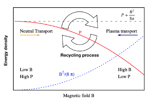
Figure 1: Plasma pressure and magnetic field energy density profiles. The recycling process can occur as shown

The transport dynamo mechanism by diffusion can be important in the laboratory plasma. In old-day Ohmic discharge experiments, it was found that a ring shape plasma initially formed near the wall, which quickly filled the center. During this process, magnetic fields of Bessel-function shapes were shown to be generated [19]. This subject will be discussed again later.

5 Necessity of additional dynamo mechanism in the mean-field dynamo theory

The mean-field dynamo theory is currently the main approach in pursuing the dynamo mechanism. In this theory, the magnetic field is generated by the nonlinear coupling of the flow velocity to the magnetic perturbation. When the field and velocity variables are decomposed into the mean and fluctuation parts, the induction equation (7) can be written as

$$\frac{\partial\overline{\mathbf{B}}}{\partial t}=\nabla\times(\overline{\mathbf{v}}\times\overline{\mathbf{B}})+\nabla\times\mathcal{E}+\frac{\eta c^{2}}{4\pi}\nabla^{2}\overline{\mathbf{B}},$$ (30)

where

$$\overline{\mathbf{v}^{\prime}}=\overline{\mathbf{B}^{\prime}}=0,$$ (31)

and

$$\mathcal{E}=\overline{\mathbf{v}^{\prime}\times\mathbf{B}^{\prime}}.$$ (32)

The overline denotes the average value, and the prime denotes the fluctuation. The electromotive force can be obtained from the average of the combined variables of velocity and magnetic fluctuations. Although the mean-field dynamo theory can explain certain dynamo activity, such as the solar butterfly diagram, there are still some concerns left about the mean-field dynamo theory.

The necessity for reconsideration or additional mechanisms to the current dynamo theory has been proposed by some authors [20, 21, 22]. One of the major drawbacks of the current dynamo theory pointed out is that it cannot adequately amplify the seed toroidal field to the desired levels [23].

The active regions of the Sun’s surface originate from strong toroidal magnetic fields that lie deep in the solar convection zone. Thin flux tube models of emerging flux loops through the solar convective envelope require a strong toroidal magnetic field at the base of the solar convection zone. Its magnetic energy is about 10 to 100 times the kinetic energy [23]. However, the mean-field dynamo theory has a difficulty in increasing the magnetic energy beyond the equipartition energy.

Ideal MHD is based on various approximations and many effects are omitted from the ideal MHD description. When the electron pressure effect becomes important, the Biermann battery can play an important role. When the electron pressure term is included, Ohm’s law (15) becomes

$$\mathbf{E}+\frac{1}{c}\mathbf{v}\times\mathbf{B}=-\frac{1}{nc}\mathbf{\Gamma}\times\mathbf{B}+\eta\mathbf{J}-\frac{\nabla{p_{e}}}{n_{e}e},$$ (33)

and this equation gives rise to the magnetic induction equation as,

$$\frac{\partial\mathbf{B}}{\partial t}-\nabla\times(\mathbf{v}\times\mathbf{B})=\nabla\times({\frac{1}{n}\mathbf{\Gamma}\times\mathbf{B}})+\frac{\eta c^{2}}{4\pi}\nabla^{2}\mathbf{B}-c\frac{\nabla{n_{e}}\times{\nabla{p_{e}}}}{{n_{e}}^{2}e}.$$ (34)

The last term in equation (34) is the Biermann battery term. Recently, Tzeferacos et al. studied the turbulent dynamo in colliding jet plasma experiments using a high-power laser and could observe the turbulent magnetic generation [24]. However, Ryu et al. pointed out by using simulation results that the Biermann battery effects may in fact have contributed more than they expected to their observed results [25]. The magnetic energy of a small-scale turbulent dynamo can be significantly affected by the Biermann battery effect. Whether the scale of magnetic generation is large or small, the search for additional dynamo mechanisms seems to be in order.

6 Exact solution for magnetic evolution

If the resistivity term in equation (16) is moved to the LHS and the flow velocity is set to be zero such that $\mathbf{v}=0$, the magnetic induction equation becomes a simple heat equation with a source term.

$$\frac{\partial\mathbf{B}}{\partial t}-\frac{\eta c^{2}}{4\pi}\nabla^{2}\mathbf{B}=\nabla\times(\frac{1}{n}\mathbf{\Gamma}\times\mathbf{B}).$$ (35)

In the absence of a source term, the homogeneous partial differential equations can be solved in cylindrical geometry using the Bessel function. The complexity of the source term on the RHS makes it difficult to solve equations analytically. However, Lee and Ryu [6, 7] have shown that if the diffusion flow velocity $v_{D}$ is of Bohm-type, analytically obtaining specific solutions is possible for magnetic fields with axial or azimuthal symmetry. By using a simple density profile and the Green’s function technique, the analytical solution for the magnetic field was obtained as follows.

$$\begin{array}[]{l}B_{z}(r,t)=B_{z}^{\mathrm{g}}(r,t)+B_{z}^{P}(r,t)\\ \quad=\sum_{m=1}^{\infty}\left[d_{m}+\int_{0}^{t}\mathrm{e}^{a\alpha_{0x}^{2}t^{\prime}/L^{2}}k_{m}\left(t^{\prime}\right)\mathrm{d}t^{\prime}\right]\mathrm{e}^{-a\alpha_{0\pi}^{2}t/L^{2}}\\ \quad\times J_{0}\left(\alpha_{0m}\frac{r}{L}\right),\end{array}$$ (36)

$$\begin{array}[]{l}B_{\theta}(r,t)=B_{\theta}^{\mathrm{g}}(r,t)+B_{\theta}^{\mathrm{P}}(r,t)\\ \quad=\sum_{m=1}^{\infty}\left[f_{m}+\int_{0}^{t}\mathrm{e}^{a\alpha_{1m}^{2}t^{\prime}/L^{2}}g_{m}\left(t^{\prime}\right)\mathrm{d}t^{\prime}\right]\mathrm{e}^{-a\alpha_{1}^{2}t/L^{2}}\\ \quad\times J_{1}\left(\alpha_{1m}\frac{r}{L}\right).\end{array}$$ (37)

Here, $\alpha_{0m}$ and $\alpha_{1m}$ are the $m$th zeroes of Bessel functions, and $\mathrm{g}$ and $P$ in the superscripts denote homogeneous and particular solutions, respectively. These results indicate that Bohm-type diffusion can amplify or reduce the magnetic field in the form of a Bessel function depending on the diffusion direction in the cylindrical approximation. For a 100 eV plasma in an apparatus of L=0.1 m with a radially increasing density profile as $n\sim exp(-x/L)$, the magnetic amplification in time becomes $(ckT/{16eL^{2})\alpha_{01}}^{2}t$ with ${\alpha_{01}=0.24}$, which becomes $3.6\times 10^{7}t$ /sec. Compared to the growth rate estimated using eq.(28), the growth rate obtained from the exact solution has an extra factor ${\alpha_{01}}^{2}$ associated with the first zero of Bessel function $J_{0}$ . The amplified magnetic field can be eventually saturated by the reduction of the diffusion coefficient due to increased magnetic fields and the decreased temperature by the increased magnetic energy.

On the other hand, if the magnetic field has dual directional components ${\mathbf{B}}={\mathbf{B}_{z}}+{\mathbf{B}_{\theta}}$, the diffusion source term becomes $\nabla\times({\mathbf{v_{D}}\times{\mathbf{B}}})=\nabla\times({\mathbf{v}_{D}}\times({\mathbf{B}_{z}}+{\mathbf{B}_{\theta}))}$, with the magnitude of the magnetic field $B=\sqrt{B_{z}^{2}+B_{\theta}^{2}}$, which determines the diffusion coefficient. Then, unlike the unidirectional the cases, the diffusion source term is no longer separable for each direction. In this case, simple growing and damping solutions cannot be obtained, and a computational study can only provide solutions for coupled magnetic induction equations. However, such a computational study is completely lacking at present.

As mentioned previously, many laboratory and astrophysical plasmas exhibit magnetic fields in the form of Bessel-functions, $J_{0}$ and $J_{1}$, in the toroidal and poloidal directions, respectively. Bessel function shaped magnetic fields have been shown to occur naturally in the force-free equilibrium,

$$\frac{1}{c}(J\times B)=0.$$ (38)

The path to this special magnetic configuration is currently thought to be due to turbulent relaxation toward the minimum energy state [26, 27], but how this relaxation can be achieved by turbulence in a deterministic system is not fully understood. Magnetic field evolution equations shown above in (36, 37) may provide further insight into this magnetic relaxation. As described above, if the magnetic evolution is governed by plasma transport, turbulence can also affect magnetic relaxation via plasma transport. This particular diffusion effect by turbulence on the magnetic evolution can be investigated in plasma devices like the Reversed Field Pinch (RFP) or the Field Reversed Configuration (FRC).

7 Conclusion

Turbulence plays an important role in the dynamo mechanism. Turbulence can generate the magnetic field through the mean-field dynamo mechanism, but inclusion of cross-field diffusion enables a new kind of dynamo mechanism. In this new mechanism, turbulence can generate magnetic fields in the following manner: turbulence induces diffusion of fluid through random motion and then generates a magnetic field through the cross-field diffusion flow. (see Figure 2)

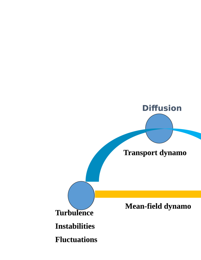
Figure 2: Turbulence can generate magnetic fields directly via mean-field dynamo and indirectly via transport dynamo. D denotes the diffusion process

Plasma diffusion across the magnetic field has been observed in many laboratory plasmas. In thermonuclear fusion plasmas, the cross-field diffusion plays an important role in plasma-confinement and thus has been intensively studied. However, the potential of diffusion flow to generate magnetic fields has been overlooked. Despite the fact that significant amounts of magnetic fields can be induced by diffusion, there is no dedicated experiment yet to measure the plasma diffusion in relation to magnetic field generation.

The generation of a magnetic field by diffusion has a few distinguishing characteristics: First, since magnetic generation is mediated by a very slow diffusion process, it can occur on a much slower time scale than the Alfvén time scale. Second, this mechanism can only occur in nonuniform situations, because there is no diffusion flow in a uniform situation. In addition, turbulence can greatly enhance the magnetic generation by increasing the diffusion coefficient. Furthermore, this process is irreversible. Therefore, the diffusion flow is completely different from the advection flow. The irreversible diffusion flow has the ability to generate magnetic fields due to its innate property of having a relative velocity to the magnetic field line. This effect is absent in the advection flow. Therefore, it can be concluded that there are two kinds of flows in MHD; advection, where bulk fluid volume moves with magnetic field lines at the same velocity, and diffusion, where fluid permeates through the magnetic field line with a relative velocity. Both satisfy Ohm’s law and flux conservation required in ideal MHD.

Plasma transport by diffusion is a widespread phenomenon in laboratory and astrophysical plasmas. Diffusion flows have the ability to generate a magnetic field. However, at present, confirming evidence is lacking. If the magnetic field could be sufficiently amplified by a transport flow, it could have significant implications for a broad range of magnetic activities in plasma. From this perspective, the transport dynamo mechanism may need more attention and more theoretical and experimental studies.

8 Acknowledgements

This work was supported by IBS (Institute for Basic Science) under the contract IBS-R012-D1.

9 References

References

- [1] Kulsrud R. 2005, Plasma Physics for Astrophysics (Princeton University Press, Princeton, NJ, 2005).
- [2] Cowling T. 1976 Magnetohydrodynamics, Chap5, p86, Adam Hilgar, Bristol.
- [3] Brandenburg A. 2018 J. Plasma Phys. 84(4) 735840404.
- [4] Ryu C.M. 1984 Los Alamos preprint, LA-UR–84-1677; Ryu C.-M. 1987 J. Astron. Space Sci. 4(2) 95.
- [5] Ryu C.M. and Yu M. 1998 Phys. Scr. 57(5) 601.
- [6] Lee T.Y and Ryu C.M. 2004 Phys. Plasmas 11 5462.
- [7] Lee T.Y. and Ryu C.M. 2007 J. Phys. D: App. Phys. 40(19) 5912.
- [8] Ryu C.M. 2019 46th EPs conference P4.4008.
- [9] Alfvén, H. (1942). ”Existence of electromagnetic-hydrodynamic waves”. Nature. 150: 405. doi:10.1038/150405d0 : Arkiv för matematik, astronomi och fysik. 29B(2): 1–7.
- [10] Haines M.G. 1981 Phys. Rev. Lett. 47 917.
- [11] Fälthammar C.-G. 2006 Am. J. Phys. 74 454.
- [12] Newcomb W.A. 1958 An. Phys. 3 358.
- [13] Bellan P. M. 2006 Fundamentals of plasma physics, (Cambridge University Press), p. 100.
- [14] Bohm, D., Burhop, E. H. S., and Massey, H. S. W. in The Characteristics of Electrical Discharges in Magnetic Fields, edited by A. Guthrie and R. K. Wakerling (McGraw‐Hill, New York, 1949), Chap. 2.
- [15] Spitzer, L., 1960 “Particle Diffusion across a Magnetic Field” , Phys. of Fluids 3, 659. doi:10.1063/1.1706104.
- [16] Chen F. 1974 introduction to Plasma Physics and Controlled FusionChap.5 (Plenum Press, New York and London.
- [17] Dawson J.M. 1983 Rev. Mod. Phys. 55 403.
- [18] Marmar E. 1978 J. Nucl. Mater. 59 450.
- [19] Lovberg R. H. 1959 Annals of Physics 8 311 DOI: 10.1016/0003-4916(59)90001-6.
- [20] Charbonneau P. 2016 Nature 535 500.
- [21] Wright N. and Drake J. 2016 Nature 535 526.
- [22] Guerrero G. and Käpylä P. 2011 A&A 533, A40.
- [23] Fan Y. Living Rev. Sol. Phys., 2009 6: 4.
- [24] Tzeferacos, P. et al. 2018 Nat. Comm. 9 (1), 591.
- [25] Ryu C.M. et al. 2019 High Energ. Dens. Phys. 3, 74.
- [26] Taylor J.B. 1974 Phys. Rev. Lett. 33 1139. doi: 10.1103/PhysRevLett.33.1139
- [27] Taylor J.B. 1986 Relaxation and magnetic reconnection in plasmas. Rev. Mod. Phys., 58:741–763, July. doi: 10.1103/RevModPhys.58.741.