Fast and Interpretable Consensus Clustering via Minipatch Learning

Abstract

Consensus clustering has been widely used in bioinformatics and other applications to improve the accuracy, stability and reliability of clustering results. This approach ensembles cluster co-occurrences from multiple clustering runs on subsampled observations. For application to large-scale bioinformatics data, such as to discover cell types from single-cell sequencing data, for example, consensus clustering has two significant drawbacks: (i) computational inefficiency due to repeatedly applying clustering algorithms, and (ii) lack of interpretability into the important features for differentiating clusters. In this paper, we address these two challenges by developing IMPACC: Interpretable MiniPatch Adaptive Consensus Clustering. Our approach adopts three major innovations. We ensemble cluster co-occurrences from tiny subsets of both observations and features, termed minipatches, thus dramatically reducing computation time. Additionally, we develop adaptive sampling schemes for observations, which result in both improved reliability and computational savings, as well as adaptive sampling schemes of features, which leads to interpretable solutions by quickly learning the most relevant features that differentiate clusters. We study our approach on synthetic data and a variety of real large-scale bioinformatics data sets; results show that our approach not only yields more accurate and interpretable cluster solutions, but it also substantially improves computational efficiency compared to standard consensus clustering approaches.

1 Introduction

Consensus clustering is a widely used unsupervised ensemble method in the domains of bioinformatics, pattern recognition, image processing, and network analysis, among others. This method often outperforms conventional clustering algorithms by ensembling cluster co-occurrences from multiple clustering runs on subsampled observations (Ghaemi et al., 2009). However, consensus clustering has many drawbacks when dealing with large data sets typical in bioinformatics. These include computational inefficiency due to repeated clustering of very large data on multiple subsamples, degraded clustering accuracy due to high sensitivity to irrelevant features, as well as a lack of interpretability. Consider, for example, the task of discovering cell types from single-cell RNA sequencing data. This data often contains tens-of-thousands of cells and genes, making consensus clustering computationally prohibitive. Additionally, only a small number of genes are typically responsible for differentiating cell types; consensus clustering considers all features and provides no interpretation of which features or genes may be important. Inspired by these challenges for large-scale bioinformatics data, we propose a novel approach to consensus clustering that utilizes tiny subsamples or minipatches as well as adaptive sampling schemes to speed computation and learn important features.

1.1 Related Work

Several types of consensus functions in ensemble clustering have been proposed, including co-association based function (Fred, 2001; Fred and Jain, 2002b; Kellam et al., 2001; Azimi et al., 2006), hyper-graph partitioning (Strehl and Ghosh, 2002; Ng et al., 2001; Karypis and Kumar, 1998), relabeling and voting approach (Dudoit and Fridlyand, 2003; Fischer and Buhmann, 2003b, a), mixture model (Topchy et al., 2004a, 2005; Analoui and Sadighian, 2007), and mutual information (Luo et al., 2006; Topchy et al., 2003; Azimi et al., 2007). Co-association based function, such as consensus clustering, is faster in convergence and is more applicable to large-scale bioinformatics data sets. Our approach is based on consensus clustering, whose concept is straightforward. In order to achieve evidence accumulation, a consensus matrix is constructed from pairwise cluster co-occurrence, ranging in $[0,1]$. It is later regarded as a similarity matrix of the observations to obtain the final clustering results (Fred and Jain, 2005). Closely related to our work, numerous variants of consensus clustering with adaptive subsampling strategies on observations have been proposed. For instance, Duarte et al. (2012) update the sampling weights of objects with their degrees of confidence, which are subtracted by clustering the consensus matrix; Parvin et al. (2013) compute sampling weights by the uncertainty of object assignments based on consensus indices’ distances to $0.5$; and Topchy et al. (2004b) adaptively subsample objects according to the consistency of clustering assignments in previous iterations. Besides adaptive sampling, Ren et al. (2017) overweight the observations with high confusion, and assigns the one-shot weights to obtain final clustering results. However, the existing sampling schemes focus on observations only and do not take feature relevance in to consideration. So these methods show inferior performance in application to sparse data sets, where only a small set of features can significantly influence cluster assignments.

Many clustering methods and pipelines have been proposed that specifically focus on single cell RNA-seq data (Kiselev et al., 2017; Yang et al., 2019; Satija et al., 2015; Wolf et al., 2018; Trapnell et al., 2014). A popular approach, SC3 (Kiselev et al., 2017), employs consensus clustering by applying dimension reduction to the subsampled data and then applying K-means. Satija et al. (2015) integrate dropout imputation and dimension reduction with a graph-based clustering algorithm. Another widely used and simple approach is to conduct tSNE dimension reduction followed by K-Means clustering (Kiselev et al., 2019). Many have discussed the computational challenge of clustering large-scale single-cell sequencing data (Kiselev et al., 2019) and have sought to address this via dimension reduction. But clustering based on dimension reduced data is no longer directly interpretable; that is, one cannot determine which genes are directly responsible for differentiating cell type clusters. The motivation of our approach is not only to develop a fast computational approach, but also to develop a method which has built-in feature interpretability to discover deferentially expressed genes.

A series of clustering algorithms have been proposed to add insights on feature importance. Some clustering algorithms conduct sparse feature selection through regularization within clustering algorithms. For example, sparse K-Means (sparseKM), sparse hierarchical clustering (spaeseHC) (Witten and Tibshirani, 2010) and sparse convex clustering (Wang et al., 2018; Wang and Allen, 2021) facilitate feature selection by solving a lasso type optimization problem. But this type of sparse clustering algorithm is often slow and highly sensitive to hyper-parameter choices; thus they face maybe computational challenges for large data. Another class of methods ranks features by their influence to results. The resulting sensitivity to the changes of one feature can be measured by the difference of silhouette widths of clustering results (Yu et al., 2019), difference of the entropy of consensus matrices (Dash and Liu, 2000), or consistency of graph spectrum (Zhao and Liu, 2007). However, feature ranking methods have to measure the importance of each feature separately, which lead to extremely high computational cost. Additionally, Liu et al. (2018) propose a post-hoc feature selection method which solves an optimization problem to determine important features within the regular consensus clustering algorithm; however, this approach suffers from major computational hurdles for large data. Therefore, we are motivated to propose an extension of consensus clustering to dramatically improve clustering accuracy, provide model interpretability, and simultaneously ease the computational burden, by incorporating innovative adaptive sampling schemes on both features and observations with minipatch learning.

1.2 Contributions

In this paper, we propose a novel methodology as an extension of consensus clustering, which demonstrates major advantages in large scale bioinformatics data sets. Specifically, we seek to improve computational efficiency, provide interpretability in terms of feature importance, and at the same time improve clustering accuracy. We achieve these goals by leveraging the idea of minipatch learning (Yao and Allen, 2020; Yao et al., 2021; Toghani and Allen, 2021) which is an ensemble of learners trained on tiny subsamples of both observations and features. Compared to only subsampling observations in existing consensus clustering ensembles, by learning on many tiny data sets, our approach offers dramatic computational savings. In addition, we develop novel adaptive sampling schemes for both observations and features to concentrate learning on observations with uncertain cluster assignments and on features which are most important for separating clusters. This provides inherent interpretations for consensus clustering and also further improves computational efficiency of the learning process. We test our novel methods and compare them to existing approaches through extensive simulations and four large real-data case studies from bioinformatics and imaging. Our results show major computational gains with our run time on the same order as that of hierarchical clustering as well as improved clustering accuracy, feature selection performance, and interpretability.

2 Minipatch Consensus Clustering

Let $\boldsymbol{X}\in\mathbb{R}^{N\times M}$ be the data matrix of interest, with $M$ features measured over $N$ observations. $\boldsymbol{x_{i}}\in\mathbb{R}^{M}$ is the $M$-dimensional feature vector observed for sample $i$. We assume that the observations can be separated into $K$ non-overlapping and exhaustive clusters; our goal is to find these clusters. We propose to extend popular consensus clustering techniques (Monti et al., 2003) to be able to more accurately and computationally efficiently detect clusters in high-dimensional noisy data common in bioinformatics (Hayes et al., 2006; Verhaak et al., 2010). We also seek ways to ensure our clusters are interpretable through feature selection. To this end, we propose a number of innovations and improvements to consensus clustering outlined in our Minipatch Consensus Clustering framework in Algorithm 1. Similar to consensus clustering, our approach repeatedly subsamples the data, applies clustering, and records the $N\times N$ co-cluster membership matrix, $\boldsymbol{\mathcal{V}}$. It then ensembles all the co-cluster membership information together into the $N\times N$ consensus matrix $\boldsymbol{\mathcal{S}}$. This consensus matrix takes values in $[0,1]$ indicating the proportion of times two observations are clustered together; it can be regarded as a similarity matrix for the observations. A perfect consensus matrix includes only entries of $0$ or $1$, where observations are always assigned to the same clusters; values in between indicate the (un)reliability of cluster assignments for each observation. To obtain final cluster assignments, one can cluster the estimated consensus matrix, which typically yields more accurate clusters than applying standard, non-ensembled clustering algorithms (Ghaemi et al., 2009).

While the core of our approach is identical to that of consensus clustering, we offer three major methodological innovations in Steps 1 and 2 of Algorithm 1 that yield dramatically faster, more accurate, and interpretable results. Our first innovation is building cluster ensembles based on tiny subsets (typically 10% or less) of both observations and features termed minipatches (Yao and Allen, 2020; Yao et al., 2021; Toghani and Allen, 2021). Note that existing consensus clustering approaches form ensembles by subsampling typically 80% of observations and all the features for each ensemble member (Wilkerson and Hayes, 2010). For large-scale bioinformatics data where the number of observations and features could be in the tens-of-thousands, repeated clustering of this large data is a major computational burden. Instead, our approach termed Minipatch Consensus Clustering (MPCC) subsamples a tiny fraction of both observations and features and hence has obvious computational advantages:

Proposition 1

The computational complexity of MPCC in Algorithm 1 is $O(mn^{2}T+N^{2})$, where $T$ is the total number of minipatches.

Since $m$ and $n$ are very small, the dominating term is the $N^{2}$ computations required to update the consensus matrix. This compares very favorably to existing consensus clustering approaches which if the default of 80% of observations are subsampled in each run, then the time complexity is $O(MN^{2}T)$, which can be very slow for both large $N$ and large $M$ datasets. On the other hand, our method is comparable in complexity to hierarchical clustering which is also $O(N^{2})$ (Murtagh, 1983), but is perhaps slower than K-Means which is $O(N)$ (Pakhira, 2014). The proof of Proposition 1 is given in Appendix A.

While MPCC offers dramatic computational improvements over standard consensus clustering, one may ask whether the results will be as accurate. We investigate and address this question from the perspective of how tiny subsamples of observations and separately features affect clustering results. First, note that if a tiny fraction of observations is subsampled, then by chance some of the clusters may not be represented; this is especially the case for large $K$ or for uneven cluster sizes. Existing consensus clustering approaches typically apply a clustering algorithm with fixed $K$ to each subsample, but this practice would prove detrimental for our approach. Instead, we propose to choose the number of clusters on each minipatch adaptively. While there are many techniques in the literature to do so that could be employed with our method (Fred and Jain, 2005, 2002a), we are motivated to choose the number of clusters very quickly with nearly no additional computation. Hence, we propose to exclusively use hierarchical clustering on each minipatch and to cut the tree at the $h$ quantile (typically set to 0.95) of the dendrogram height to determine the number of clusters and cluster membership. This approach is not only fast but adaptive to the number of clusters present in the minipatch, and results change smoothly with cuts at different heights. Our empirical results reveal that this approach performs well on minipatches and we specifically investigate its utility, sensitivity, and tuning of $h$ in Appendix F; importantly, we find that setting $h=.95$ to nearly universally yields the best results and hence we suggest fixing this value. Additionally, we provide details on hyper-parameters, tuning, and stopping criteria in Appendix F.

Next, one may ask how subsampling the features in minipatches affects clustering accuracy. Obviously for high-dimensional data in which only a small number of features are relevant for differentiating clusters, subsampling minipatches containing the correct features would improve results. We address such possibilities in the next section. But if this is not the case, would clustering accuracy suffer? Since we apply hierarchical clustering which takes distances as input, we seek to understand how far off our distance input can be when we employ sub-samples of features. To this end, we consider distances that can be written in the form of the sum; this includes popular distances like the Manhattan or squared Euclidean distance, among others. The following result probabilistically bounds the deviations of the distances computed using only a subset of features:

Proposition 2

For $\epsilon>0$ and $|\hat{d}_{i,i^{\prime}}-d^{*}_{i,i^{\prime}}|\in[0,1]$, $P\left(|\hat{d}_{i,i^{\prime}}-d^{*}_{i,i^{\prime}}|\geq\epsilon\right)\leq 2\exp\left(\frac{-2m\epsilon^{2}}{(1-\frac{m-1}{M})}\right)$,

where $d_{i,i^{\prime}}^{*}=\frac{1}{M}f(x_{i},x_{i^{\prime}})$ is the distance between observations $x_{i}$ and $x_{i^{\prime}}$ using the full set of $M$ features, and $\hat{d}_{i,i^{\prime}}=\frac{1}{m}\sum_{j\in{j_{1},...,j_{m}}}f(x_{i,j},x_{i^{\prime},j})$ is the distance using a subset of $m$ features. This is derived from the Hoeffding inequality (Serfling, 1974). This result states that the probability that distances computed on minipatches are far off from original distances is small, under the worst-case scenario. This provides some reassurances that clustering accuracy based on subsampling features should not greatly suffer. While smaller minipatches yield faster computations, there may be a slight trade-off in terms of clustering accuracy. Our empirical results in Appendix F suggest that such a trade-off is generally slight or negligible, so we can typically utilize smaller minipatches.

  Input: $\boldsymbol{X}$, $n$, $m$, $\boldsymbol{\mathcal{V}}^{(0)}$, $\boldsymbol{\mathcal{D}}^{(0)}$, $h$;

while stopping criteria not meet do

       1. Obtain minipatch $\boldsymbol{X}_{I_{t},F_{t}}$ $\in\mathbb{R}^{n\times m}$ by subsampling $n$ observations $I_{t}\subset\{1,...,N\}$ and $m$ featrues $F_{t}\subset\{1,...,M\}$, without replacement; • MPCC subsamples uniformly at random; • MPACC uses the adaptive observation sampling scheme only; • IMPACC uses both adaptive feature and observation sampling schemes simultaneously; 2. Obtain estimated clustering result $\mathcal{C}^{(t)}$ by fitting hierarchical clustering to $\boldsymbol{X}_{I_{t},F_{t}}$ and cut tree at $h$ height quantile; 3. Update co-clustering membership matrix $\boldsymbol{\mathcal{V}}$ and co-sampling matrix $\boldsymbol{\mathcal{D}}$: $\boldsymbol{\mathcal{V}}^{(t)}(i,i^{\prime})=\boldsymbol{\mathcal{V}}^{(t-1)}(i,i^{\prime})+\mathbb{I}(\mathcal{C}^{t}_{i}=\mathcal{C}^{t}_{i^{\prime}});\quad\boldsymbol{\mathcal{D}}^{(t)}(i,i^{\prime})=\boldsymbol{\mathcal{D}}^{(t-1)}(i,i^{\prime})+\mathbb{I}(i\in I_{t},i^{\prime}\in I_{t}))$;

end while

Calculate consensus matrix $\boldsymbol{\mathcal{S}}(i,i^{\prime})=\frac{\boldsymbol{\mathcal{V}}^{(T)}(i,i^{\prime})}{\max(1,\boldsymbol{\mathcal{D}}^{(T)}(i,i^{\prime}))}$;

Obtain final clustering result $\hat{\Pi}$ by using $\boldsymbol{\mathcal{S}}$ as a similarity matrix;

Output: $\boldsymbol{\mathcal{S}}$, $\hat{\Pi}$. 

Algorithm 1 Minipatch Consensus Clustering

We have introduced minipatch consensus clustering (MPCC) using random subsamples of both features and observations. The advantage of this approach is its computational speed, which our empirical results in Section 3 suggest is on the order of standard clustering approaches such as hierarchical and spectral clustering (hence confirming Proposition 1). But, one may ask whether clustering results can be improved by perhaps optimally sampling observations and/or features instead of using random sampling. Some have suggested such possibilities in the context of consensus clustering (Duarte et al., 2012; Parvin et al., 2013; Topchy et al., 2004b; Ren et al., 2017); we explore it and develop new approaches for this in the following sections.

2.1 Minipatch Adaptive Consensus Clustering (MPACC)

One may ask whether it is possible to improve upon minipatch consensus clustering in terms of both speed and clustering accuracy by adaptively sampling observations. For example, we may want to sample observations that are not well clustered more frequently to learn their cluster assignments faster. In the method MiniPatch Adaptive Consensus Clustering (MPACC), we propose to dynamically update sampling weights, with a focus on observations that are difficult to be clustered and that are less frequently sampled. In addition, we leverage the adaptive weights by designing a novel observation sampling scheme.

Input: $\boldsymbol{\mathcal{S}}^{(t-1)}$, $\{I_{l}\}_{l=1}^{t-1}$, $\alpha_{I}$;

1. Calculate sample uncertainty $\boldsymbol{u}_{i}=\frac{1}{N}\sum_{i^{\prime}=1}^{N}\boldsymbol{\mathcal{S}}^{(t-1)}_{i,i^{\prime}}(1-\boldsymbol{\mathcal{S}}^{({t-1})}_{i,i^{\prime}})\times\frac{t-1}{\sum_{l=1}^{t-1}\mathbb{I}(i\in I_{l})}$;

2. Update observation weight vector $\boldsymbol{w_{I}}^{(t)}=\alpha_{I}\boldsymbol{w_{I}}^{(t-1)}+(1-\alpha_{I})\frac{\boldsymbol{u}}{\sum_{i=1}^{N}\boldsymbol{u}_{i}}$;

Output: $\boldsymbol{w_{I}}^{(t)}$.

Algorithm 2 Weight updating in adaptive observation sampling scheme

Specifically, we propose to dynamically update observations weights by adjusted confusion values. To measure the level of clustering uncertainty, confusion values are derived from consensus matrix, given by $confusion_{i}=\frac{1}{N}\sum_{i^{\prime}=1}^{N}\boldsymbol{\mathcal{S}}_{i,i^{\prime}}(1-\boldsymbol{\mathcal{S}})_{i,i^{\prime}}$ for observation $i$. A larger confusion value near $0.25$ indicates poorer clustering with unstable assignments, and the minimum confusion value $0$ suggests perfect clustering. Note that confusions tend to grow with iterations because more consensus values are updated from the initial value $0$. Therefore, a large confusion value due to oversampling cannot truly reflect the level of uncertainty. To eliminate bias caused by oversampling and to upweight less frequently sampled observations, we further adjust confusion values by sampling frequencies of observations in previous iterations, as presented in Algorithm 2.

The next question is, how do we leverage the weights to dynamically construct minipatches as the number of iterations grows? One simple solution is to probabilistically subsample with probability ($Prob$) proportional to the weights. But the problem with this approach is that the clustering performance will be compromised if we only tend to sample uncertain and difficult observations. To resolve such drawback, we develop an exploitation and exploration plus probabilistic ($EE+Prob$) sampling scheme (Algorithm 3). The scheme consists of two sampling stages: a burn-in stage and an adaptive stage. The purpose of the burn-in stage is to explore the entire observation space and ensure every observation is sampled several times. During the next adaptive stage, observations with the levels of uncertainty greater than a threshold are classified into the high uncertainty set, and the algorithm exploits this set by sampling $\gamma^{(t)}$ proportion of observations using probabilistic sampling. Here, $\gamma^{(t)}\in[0.5,1]$ is a monotonically increasing parameter that controls sampling size in the exploitation and exploration step. Meanwhile, the algorithm explores the rest of observations with uniform weights, to avoid exclusively focusing on difficult observations. The reason why we randomly sample the observations that we are confident about is that, we need to include a fair amount of easy-to-cluster observations to construct well-defined clusters in each minipatch so as to better cluster the uncertain ones. We also propose to use the $EE+Prob$ scheme as our adaptive feature sampling scheme, which is discussed in Section 2.2.

Input:$t$, $n$, $N$, $E$, $\{\gamma^{(t)}\}$, $\boldsymbol{w_{I}}^{(t-1)}$, $\{\tau\}$;

Initialization:$Q=[\frac{N}{n}]$, $\mathcal{I}=\{1,...,N\}$; 

if $t\leq E\cdot Q$ then

       // Burn-in stage

      if $mod_{Q}(t)=1$ then

             // New epoch

            Randomly reshuffle feature index set $\mathcal{I}$ and partition into disjoint sets $\{\mathcal{I}_{q}\}_{q=0}^{Q-1}$; 

      else

            

            Set $I_{t}=\mathcal{I}_{mod_{Q}(t)}$; 

       end if

      

else

      // Adaptive stage

      

Update observation weights $\boldsymbol{w_{I}}^{(t)}$ by Algorithm 2; 2. Create high uncertainty set $\mathcal{H}_{I}=\{i\in\{1,...,N\}:\boldsymbol{w_{I}}^{(t)}_{i}>{\tau_{\boldsymbol{w_{I}}^{(t)}}}\}$; 3. Exploitation: sample $\min(n,\gamma^{(t)}|\mathcal{H}_{I}|)$ observations $I_{t,1}\subseteq\mathcal{H}_{I}$ with probability $\boldsymbol{w_{I}}_{\mathcal{H}_{I}^{t}}$; 4. Exploration: sample $(n-\min(n,\gamma^{(t)}|\mathcal{H}|_{I}))$ observations $I_{t,2}\subseteq\{1,...,N\}\backslash\mathcal{H}_{I}$ uniformly at random; 5. Set $I_{t}=I_{t,1}\cup I_{t,2}$;

end if

Output: $I_{t}$.

 

Algorithm 3 Adaptive Observation (Features) Sampling Scheme - $EE+Prob$

2.1.1 Relation to Existing Literature

Several have suggested similar weight updating approaches in the consensus clustering literature. Ren et al. (2017) also obtain observation weights by confusion values as in our method. The difference is that, their methods only use the weight scheme at the final clustering step rather than adaptive sampling. On the other hand, similar to our adaptive weight updating scheme, Duarte et al. (2012); Topchy et al. (2004b); Parvin et al. (2013) iteratively update weights depending on clustering history. However, these existing methods utilize probabilistic sampling, so they would largely suffer from biased sampling and inaccurate results by only focusing on hard observations. However, instead of probabilistic sampling, we design the $EE+Prob$ sampling scheme to leverage the weights, which is inspired by the exploration and exploitation ($EE$) scheme from multi-arm bandits (Bouneffouf and Rish, 2019; Slivkins, 2019) and also employed for feature selection with minipatches in Yao and Allen (2020). Compared to the latter, the innovation in our approach is to combine the advantages of probabilistic sampling and exploitation-exploration sampling which proves to have particular advantages for clustering. Comparisons with other possible sampling schemes proposed in the literature are shown in Appendix F.

2.2 Interpretable Minipatch Adaptive Consensus Clustering (IMPACC)

One major drawback of consensus clustering is that it lacks interpretability into important features. This is especially important for high-dimensional data like that in bioinformatics where we expect only a small subset of features to be relevant for determining clusters. To address this, we develop a novel adaptive feature sampling approach termed Interpretable Minipatch Adaptive Consensus Clustering (IMPACC) that learns important features for clustering and hence improves clustering accuracy for high-dimensional data. In clustering, two types of approaches to determine important features have been proposed. One is to obtain a sparse solution by solving an optimization problem (Witten and Tibshirani, 2010; Wang et al., 2018; Wang and Allen, 2021), and another one is to rank features by their influence to results (Yu et al., 2019; Dash and Liu, 2000; Zhao and Liu, 2007). However, in data sets with a large number of observations and features, both kinds of methods suffer from significant computational inefficiency. So the question we are interested in is, can we achieve fast, accurate and reliable feature selection within the consensus clustering process with minipatches? We address this question by proposing a novel adaptive feature weighting method that measures the feature importance in each minipatch and then ensembles the results to increase the weights of the important features. Given these adaptive feature weights, we can then utilize our adaptive sampling scheme proposed in Algorithm 3 to more frequently sample important features.

Outlined in Algorithm 4, we propose an adaptive feature weighting scheme by testing whether each feature is associated with the estimated cluster labels on that minipatch. To do so, we use a simple ANOVA test in part, because it is computationally fast and only requires one matrix multiplication. Based on the p-values from these tests, we establish an important feature set, $A$, and obtain the importance scores as the frequency of features being classified into this feature set over iterations. Then the feature sampling weights are dynamically updated with learning rate $\alpha_{F}$. Therefore, by ensembling feature importance obtained from each iteration, we are able to simultaneously improve clustering accuracy and build model interpretability from resulting feature weights, with minimal sacrifices in terms of computational time.

 

Input: $\boldsymbol{X}_{I_{t},F_{t}}$, $\mathcal{C}^{(t-1)}$, $\{F_{l}\}_{l=1}^{t-1}$, $\{A^{l}\}_{l=1}^{t-2}$, $\{\eta\}$, $\boldsymbol{w_{F}}^{(t-1)}$, $\alpha_{F}$;

For each feature $j\in F_{t-1}$, conduct ANOVA test between features $j$ and $\mathcal{C}^{(t-1)}$, record p-value $p_{j}^{(t-1)}$;

Create a feature support $A^{(t-1)}\subseteq F_{t-1}$: $A^{(t-1)}=\{j\in\{1,...,m\}:p^{(t-1)}_{j}<\eta_{p^{(t-1)}}\}$;

Update feature weight vector $\boldsymbol{w_{F}}^{(t+1)}\in\mathbb{R}^{M}$ by ensembling feature supports $\{A^{l}\}_{l=1}^{(t-1)}$:

$$\boldsymbol{w_{F}}_{j}^{(t)}=\alpha_{F}\boldsymbol{w_{F}}_{j}^{(t-1)}+(1-\alpha_{F})\frac{\sum\limits_{l=1}^{t-1}\mathbb{I}(j\in F_{l},j\in{A}^{l})}{\max(1,{\sum\limits_{l=1}^{t-1}}\mathbb{I}(j\in F_{l}))};$$

Output: $\boldsymbol{w_{F}}^{(t)}$.

Algorithm 4 Weight updating in adaptive feature sampling scheme

We propose to utilize the same type of $EE+Prob$ sampling scheme (Algorithm 3) given our feature weights to learn the important features for clustering. Such a scheme exploits the important features and samples these more frequently as the algorithm progress. But it also balances exploring other features to ensure that potentially important features are not missed. Our final IMPACC algorithm then utilizes both adaptive observation sampling and adaptive feature sampling to both improve computation and clustering accuracy while also providing feature interpretability. Utilizing minipatches in consensus clustering allows us to develop these innovative adaptive sampling schemes and be the first to propose feature learning in this context.

Even though IMPACC has several hyper-parameters, in practice, our methods are quite robust and reliable to parameter selections, and generally give a strong performance under default parameter settings. Therefore, we are freed from the computationally expensive hyper-parameter tuning process and its computational burdens. We include a study on learning accuracy with different levels of hyper-parameters, the default values, and also suggest a data-driven tuning process in Appendix F.

Overall, the proposed MPACC with only adaptive sampling on observation is more suitable for data of no or little sparsity; and IMPACC, which adaptively subsamples both observations and features in minipatch learning, can be more useful when dealing with high dimensional and sparse data set in bioinformatics. It enhances model accuracy, scalability, and interpretability, by focusing on uncertain observations and important features in an efficient manner. Our empirical study in Section 3 demonstrates the major advantages of the IMPACC method in terms of clustering quality, feature selection accuracy and computation saving.

3 Empirical Studies

In this section we assess the performance of IMPACC and MPCC with application to a high dimensional and high noise synthetic simulation study in Section 3.1 and four large-scale real data sets in Section 3.2 , in comparison with several conventional clustering strategies.

3.1 Synthetic Data

We evaluate the performance of MPCC and IMPACC in terms of clustering accuracy and computation time with widely used competitors, and compare IMPACC’s feature selection accuracy with the existing sparse feature selection techniques. Simulations are conducted under three scenarios: sparse, weak sparse and no sparse. We only show the results of sparse simulation, as it is the best representative of high dimensional bioinformatics data, and results of the other two scenarios can be found in Appendix C.

In the sparse simulation study, each data set is created from a mixture of Gaussian with block-diagonal covariance matrix $\Sigma=\textbf{I}_{\frac{M}{5},\frac{M}{5}}\otimes(\rho\cdot\textbf{1}_{5}\cdot\textbf{1}_{5}^{T}+(1-\rho)\cdot\textbf{I}_{5,5})$, where $\otimes$ denotes the Kronecker product. The parameter $\rho$ is set to be $0.5$. We set the number of observations, features and clusters to be $N=500$, $M=5,000$, $K=4$, respectively, and the numbers of observations in each cluster are $20$, $80$, $120$, $280$. The means of features in synthetic data is $\mu=[\mu_{k},\mu_{0}]$, where $\mu_{k}\in\mathbb{R}^{25}$ and $\mu_{0}=\textbf{0}_{4975}$ are the means of $25$ signal features and $4,975$ noise features, respectively. The signal-to-noise (SNR) ratio is defined as the L2-norm of feature means: $SNR=\|\mu\|_{2}$. In order to assess feature selection capability, synthetic data is generated with $SNR$ ranging from 1 to 8. Specifically, the signal features are generated with $\mu_{1}=\frac{SNR}{5}\cdot\textbf{1}_{25}$, $\mu_{2}=(\frac{SNR}{5}\cdot\textbf{1}_{13}^{T},-\frac{SNR}{5}\cdot\textbf{1}_{12}^{T})^{T}$, $\mu_{3}=(-\frac{SNR}{5}\cdot\textbf{1}_{13}^{T},\frac{SNR}{5}\cdot\textbf{1}_{12}^{T})^{T}$, $\mu_{4}=-\frac{SNR}{5}\cdot\textbf{1}_{25}$. Data with higher SNR ratio has more informative signal features so is easier to be clustered. For all clustering algorithms, we assume oracle number of clusters $K$. Hierarchical clustering is applied as the final algorithm in IMPACC and MPCC, with number of iterations determined by an early stopping criteria, as described in Appendix B. And we have exactly the same setting as those of MPCC in regular consensus clustering, including the number of iterations. Ward’s minimum variance method with Manhattan distance is used in all hierarchical clustering related methods.

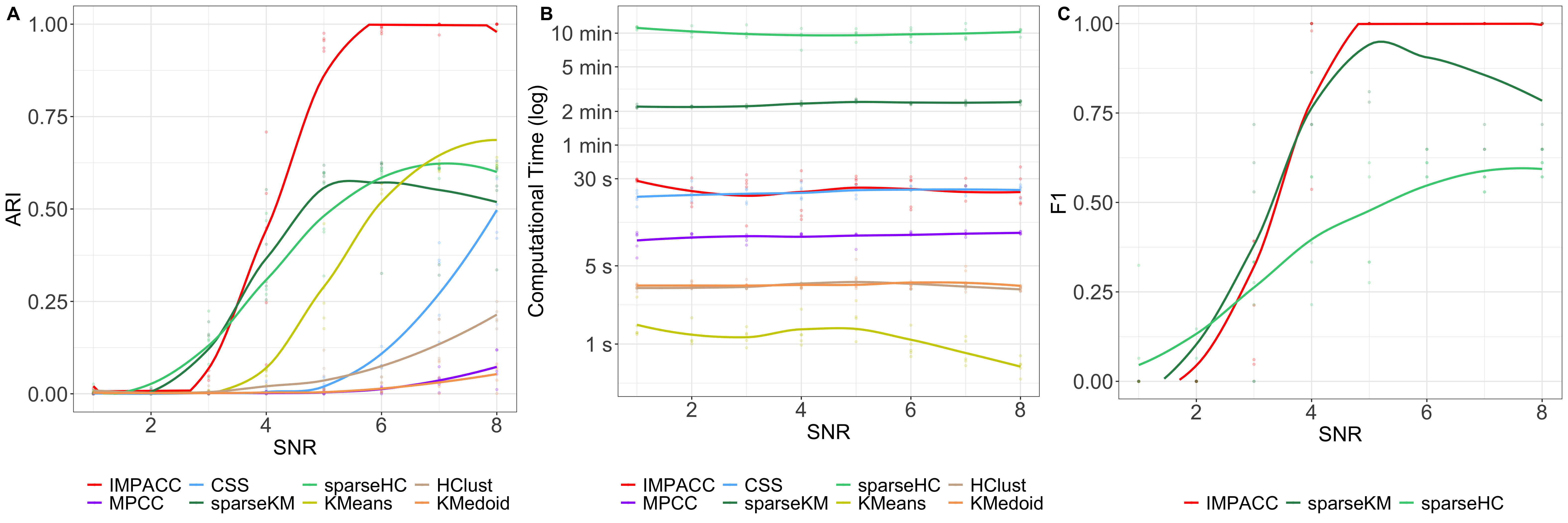
Figure 1: Clustering performance (ARI), feature selection accuracy (F1 score), and computation time on sparse synthetic data sets. (A) ARI (higher is better) of estimated grouping; (B) computation time in log seconds; (C) F1 score for signal feature estimates. IMPACC has superior performance over competing methods in clustering and feature selection accuracy with significant computation saving.

We use adjusted rand index (ARI) to evaluate the clustering performance, and F1 score to measure feature selection accuracy, which both range in $[0,1]$, with a higher value indicating higher accuracy. The averaged results over 10 repetitions are shown in Figure 1. Overall, IMPACC yields the best clustering performance over all competing methods with the highest ARI in most of the $SNR$ settings. Comparing feature selection performance, IMPACC has perfect recovery on informative features, with an F1 score equaling to $1$ when $SNR$ is large, and is significantly better than sparseKM and sparseHC. Additionally, IMPACC achieves significantly major computational advantages comparing to sparse feature selection clustering strategies. All of the computation time is recorded on a laptop with 16GB of RAM (2133 MHz) and a dual-core processor (3.1 GHz). Note that we only show results of the sparse simulation scenario in Figure 1, and we include the other two scenarios in Appendix C. Our methods are still dominant in noisy and weak sparse situations, but IMAPCC shows little improvement on the no-sparsity scenario when all the features are relevant.

3.2 Case Studies on Real Data

We apply our methods to three RNA-seq data sets and one image data set with known cluster labels, whose information is reported in Table 1. In the RNA-seq data, gene expressions are transformed by $x\mapsto\log_{2}(1+x)$ before conducting clustering algorithms; the image data set is adjusted to be within the range $[0,1]$. With the same settings in Section 3.1, we evaluate the learning performance of MPCC and IMPACC with existing methods, with the number of clusters being oracle.

	PANCAN	Brain	Neoplastic	COIL20
Data type	RNA-seq	scRNA-seq	scRNA-seq	Image
Tissue	tumor cells	brain cells	neoplastic infiltrating cells
# clusters	5	4	7	20
# observations	761	366	3,576	1,440
# features	13,244	21,413	28,805	1,024
% zeros	14.2%	80.06%	81.36%	34.38%
citation	Weinstein et al. (2013)	Darmanis et al. (2015)	Darmanis et al. (2017)	Nene et al. (1996)
GEO accession code	GSE43770	GSE67835	GSE84465

Table 1: Data sets used in empirical study.

Table 2 summarizes clustering results on real data sets. IMPACC consistently outperforms all competing methods at discovering known clusters with the highest ARI score, and it demonstrates major computational advantages, sometimes even beating hierarchical clustering. Clustering followed by dimension reduction via tSNE can have faster and better clustering accuracy for some of the data sets, but they fail to provide interpretability in terms of feature importance. Even though single cell RNA-seq specific methods Seurat and CS3 have comparable accuracy in the brain data set, these methods select genes with high variance before performing clustering algorithm and do not provide inherent interpretations of important genes. Note that R failed to apply sparseHC to large genomics data due to excessive demand on computing memory. Further, even though MPCC has slightly lower ARI than IMPACC, it still yields better performance in learning accuracy over consensus and standard methods, and it achieves the fastest computational speed over all other methods in most of the data sets, excluding K-Means clustering. Additionally, we visualize the consensus matrices of IMPACC and compare to that of regular consensus clustering in Figure 2. We can conclude that IMPACC is able to produce more accurate consensus matrices, with clearer diagonal blocks of clusters and less noise on off-diagonal entries.

	ARI				Time (s)
	PANCAN	brain	neoplastic	COIL20	PANCAN	brain	neoplastic	COIL20
IMPACC (HC)	0.939	0.978	0.908	0.744	18.491	29.204	1843.033	115.119
IMPACC (Spec)	0.828	0.924	0.856	0.711
MPCC (HC)	0.922	0.844	0.808	0.715	13.021	9.631	2170.650	91.319
MPCC (Spec)	0.833	0.804	0.842	0.67
Consensus (HC)	0.761	0.610	0.398	0.719	88.380	30.787	8866.810	1730.019
Consensus (Spec)	0.770	0.548	0.534	0.665
sparseKM	0.784	0.961	0.486	0.459	1236.009	375.658	62580.775	207.68
sparseHC	N/A	0.247	N/A	0.158	N/A	1540.236	N/A	1867.174
KMeans	0.797	0.588	0.513	0.542	2.154	1.558	97.083	0.305
KMedoid	0.795	0.255	0.160	0.532	30.494	12.261	6063.345	9.079
HClust	0.769	0.613	0.413	0.688	28.016	13.835	6052.748	6.274
Spectral	0.776	0.575	0.671	0.561	19.640	7.561	1463.087	69.546
tSNE+KMeans	0.863	0.702	0.346	0.614	29.222	15.008	1577.265	8.859
tSNE+KMedoid	0.960	0.944	0.342	0.740	29.390	15.023	1582.872	13.138
tSNE+HClust	0.990	0.950	0.445	0.760	29.240	15.001	1577.719	8.906
tSNE+Spectral	0.789	0.726	0.725	0.641	44.824	17.541	3126.325	121.169
Seurat		0.908	0.683			4.285	25.019
CS3		0.978	0.453			134.920	1486.074

Table 2: Clustering performance (ARI) and computation time in seconds on real data sets with known cluster labels. The IMPACC method outperforms others in clustering performance, with significant improvements on computational cost compared to sparseKM, sparseHC and consensus clustering. The MPCC method also yields comparable clustering performance, and achieves the fastest computational speed excluding K-Means clustering.

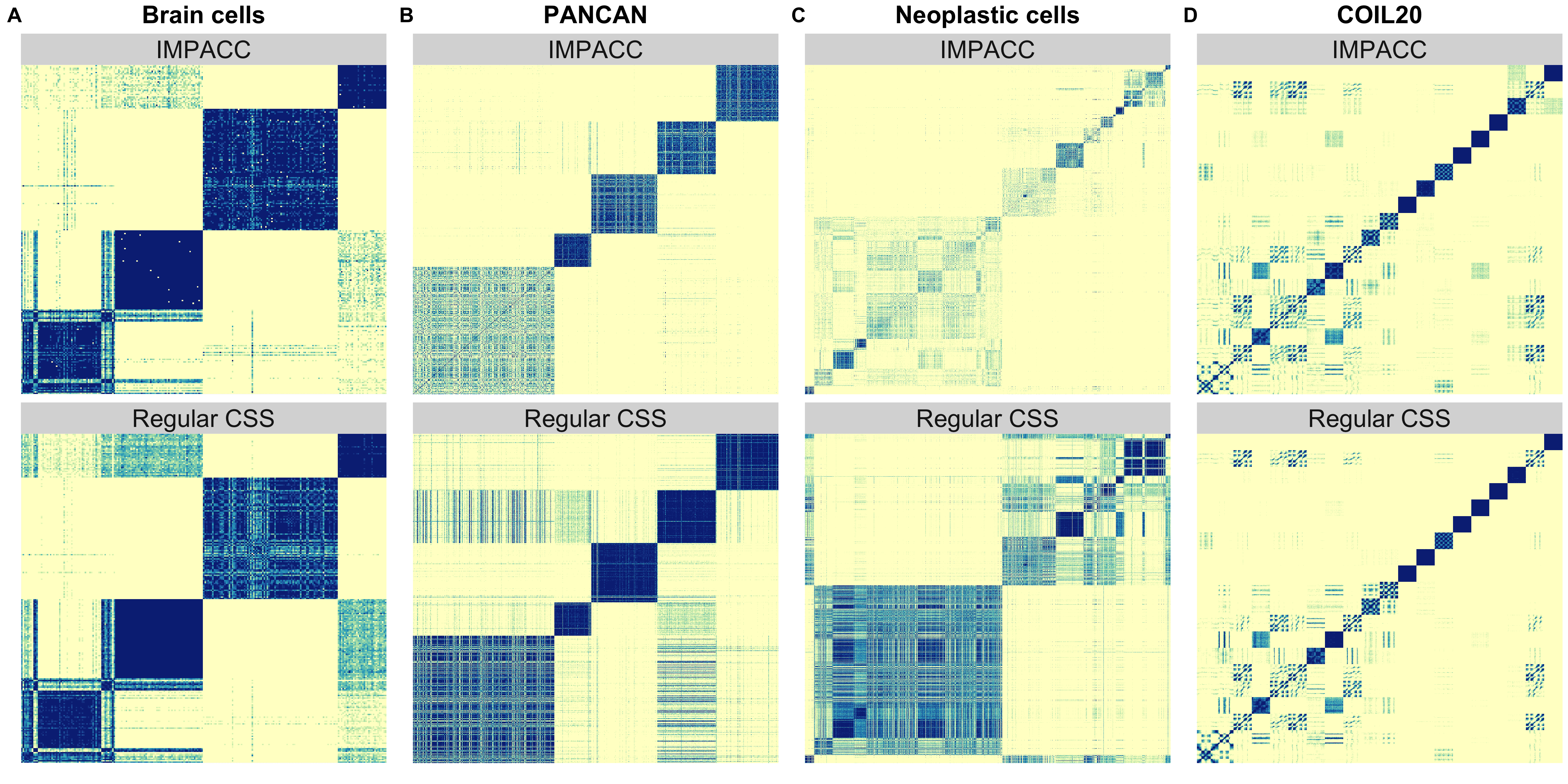
Figure 2: Heatmaps of final consensus matrix derived from IMPACC and consensus clustering respectively, using oracle number of clusters. Darker color indicates higher consensus value.

IMPACC further provides interpretablility in terms of feature importance. 19 of top 25 genes with high importance (feature score $\in[0.78,1]$) in brain cell data set are enriched/enhanced in brain; in top 25 genes (feature score $\in[0.933,1]$) in the PANCAN tumor data set, 11 genes are prognostic cancer markers and 13 are enriched/enhanced in tissues; 9 of the top 25 genes (feature score $\in[0.52,1])$ in neoplastic cells are enriched in the brain, and 17 genes are prognostic cancer markers. For example, BCAN is highly relevant to tumor cell migration with contribution to nervous system development, and OPALIN is a known marker in oligodendrocytes (Darmanis et al., 2017). The gene information is sourced from the Human Protein Atlas (Pontén et al., 2008), and more details on significant genes can be found in Appendix D.

To further evaluate the model interpretability of IMPACC, sparseKM and sparseHC, we perform pathway analysis on the most important genes discovered by each method. We determined genes as important if their feature importance scores were higher than the mean plus one standard deviation of all scores. IMPACC is able to identify a larger set of important genes with more discrepancy between signal and noise genes. By performing KEGG pathway analysis, we find the important genes obtained from IMPACC are enriched in much more biological meaningful pathways with smaller p-values, comparing to those identified by sparseKM and sparseHC. For example, as shown in Table  3, $578$, $89$ and $27$ important genes are detected by IMPACC, sparseKM and sparseHC, respectively in the brain cell data. The top enriched KEGG pathways from IMPACC is GABAergic synapse, which is the main neurotransmitter in adult mammalian brain (Watanabe et al., 2002). Therefore, IMPACC provides accurate and reliable interpretations on scientifically important genes. Additional pathway analyses are detailed in Appendix D .

	IMAPCC			sparseKM			sparseHC
	Pathway	Name	p-value	Pathway	Name	p-value	Pathway	Name	p-value
1	hsa04727	GABAergic synapse	2.357e-15	hsa04964	Proximal tubule bicarbonate reclamation	1.3191e-07	hsa04976	Bile secretion	0.0011
2	hsa04911	Insulin secretion	1.457e-12	hsa04727	GABAergic synapse	8.602e-06	hsa04964	Proximal tubule bicarbonate reclamation	0.0013
3	hsa04721	Synaptic vesicle cycle	2.208e-12	hsa04976	Bile secretion	0.0001	hsa04724	Glutamatergic synapse	0.0022
4	hsa04978	Mineral absorption	3.492e-09	hsa04978	Mineral absorption	0.0003	hsa04919	Thyroid hormone signaling pathway	0.0027
5	hsa04971	Gastric acid secretion	1.121e-08	hsa04919	Thyroid hormone signaling pathway	0.00052	hsa01230	Biosynthesis of amino acids	0.0131

Table 3: Top 5 enriched KEGG pathways in brain cell data set

4 Discussion

We have proposed novel and powerful methodologies for consensus clustering using minipatch learning with random or adaptive sampling schemes. We have demonstrated that both MPCC and IMPACC are stable, robust, and offer superior performance than competing methods in terms of computational accuracy. Further, the approaches offer dramatic computational savings with runtime comparable to hierarchical or spectral clustering. Finally, IMPACC offers interpretable results by discovering features that differentiate clusters. This method is particularly applicable to sparse, high-dimensional data sets common in bioinformatics. Our empirical results suggest that our method might prove particularly important for discovering cell types from single-cell RNA sequencing data. Note that while our methods offer computational advantages over consensus clustering for all settings, our method does not seem to offer any dramatic improvement in clustering accuracy for non-sparse and non-high-dimensional data sets. In future work, one can further optimize computations through memory-efficient management of the large consensus matrix and through hashing or other approximate schemes. Overall, we expect IMPACC to become a critical instrument for clustering analyses of complicated and massive data sets in bioinformatics as well as a variety of other fields.

Funding

This work has been supported by NSF DMS-1554821 and NIH 1R01GM140468.

Conflict of Interest: none declared.

References

- Analoui and Sadighian [2007] Morteza Analoui and Niloufar Sadighian. Solving cluster ensemble problems by correlation’s matrix & ga. In Intelligent Information Processing III: IFIP TC12 International Conference on Intelligent Information Processing (IIP 2006), September 20–23, Adelaide, Australia 3, pages 227–231. Springer, 2007.
- Azimi et al. [2006] Javad Azimi, Mehdi Mohammadi, Morteza Analoui, et al. Clustering ensembles using genetic algorithm. In 2006 International Workshop on Computer Architecture for Machine Perception and Sensing, pages 119–123. IEEE, 2006.
- Azimi et al. [2007] Javad Azimi, Monireh Abdoos, and Morteza Analoui. A new efficient approach in clustering ensembles. In International Conference on Intelligent Data Engineering and Automated Learning, pages 395–405. Springer, 2007.
- Bouneffouf and Rish [2019] Djallel Bouneffouf and Irina Rish. A survey on practical applications of multi-armed and contextual bandits. arXiv preprint arXiv:1904.10040, 2019.
- Darmanis et al. [2015] Spyros Darmanis, Steven A Sloan, Ye Zhang, Martin Enge, Christine Caneda, Lawrence M Shuer, Melanie G Hayden Gephart, Ben A Barres, and Stephen R Quake. A survey of human brain transcriptome diversity at the single cell level. Proceedings of the National Academy of Sciences, 112(23):7285–7290, 2015.
- Darmanis et al. [2017] Spyros Darmanis, Steven A Sloan, Derek Croote, Marco Mignardi, Sophia Chernikova, Peyman Samghababi, Ye Zhang, Norma Neff, Mark Kowarsky, Christine Caneda, et al. Single-cell rna-seq analysis of infiltrating neoplastic cells at the migrating front of human glioblastoma. Cell reports, 21(5):1399–1410, 2017.
- Dash and Liu [2000] Manoranjan Dash and Huan Liu. Feature selection for clustering. In Pacific-Asia Conference on knowledge discovery and data mining, pages 110–121. Springer, 2000.
- Duarte et al. [2012] João MM Duarte, Ana LN Fred, and F Jorge F Duarte. Adaptive evidence accumulation clustering using the confidence of the objects’ assignments. In Pacific-Asia Conference on Knowledge Discovery and Data Mining, pages 70–87. Springer, 2012.
- Dudoit and Fridlyand [2003] Sandrine Dudoit and Jane Fridlyand. Bagging to improve the accuracy of a clustering procedure. Bioinformatics, 19(9):1090–1099, 2003.
- Fischer and Buhmann [2003a] B. Fischer and J.M. Buhmann. Bagging for path-based clustering. IEEE Transactions on Pattern Analysis and Machine Intelligence, 25(11):1411–1415, 2003a. doi:10.1109/TPAMI.2003.1240115.
- Fischer and Buhmann [2003b] Bernd Fischer and Joachim M. Buhmann. Path-based clustering for grouping of smooth curves and texture segmentation. IEEE Transactions on Pattern Analysis and Machine Intelligence, 25(4):513–518, 2003b.
- Fred [2001] Ana Fred. Finding consistent clusters in data partitions. In International Workshop on Multiple Classifier Systems, pages 309–318. Springer, 2001.
- Fred and Jain [2002a] Ana Fred and Anil K Jain. Evidence accumulation clustering based on the k-means algorithm. In Joint IAPR International Workshops on Statistical Techniques in Pattern Recognition (SPR) and Structural and Syntactic Pattern Recognition (SSPR), pages 442–451. Springer, 2002a.
- Fred and Jain [2002b] Ana LN Fred and Anil K Jain. Data clustering using evidence accumulation. In Object recognition supported by user interaction for service robots, volume 4, pages 276–280. IEEE, 2002b.
- Fred and Jain [2005] Ana LN Fred and Anil K Jain. Combining multiple clusterings using evidence accumulation. IEEE transactions on pattern analysis and machine intelligence, 27(6):835–850, 2005.
- Ghaemi et al. [2009] Reza Ghaemi, Md Nasir Sulaiman, Hamidah Ibrahim, Norwati Mustapha, et al. A survey: clustering ensembles techniques. World Academy of Science, Engineering and Technology, 50:636–645, 2009.
- Hayes et al. [2006] D Neil Hayes, Stefano Monti, Giovanni Parmigiani, C Blake Gilks, Katsuhiko Naoki, Arindam Bhattacharjee, Mark A Socinski, Charles Perou, and Matthew Meyerson. Gene expression profiling reveals reproducible human lung adenocarcinoma subtypes in multiple independent patient cohorts. Journal of Clinical Oncology, 24(31):5079–5090, 2006.
- Karypis and Kumar [1998] George Karypis and Vipin Kumar. A fast and high quality multilevel scheme for partitioning irregular graphs. SIAM Journal on scientific Computing, 20(1):359–392, 1998.
- Kellam et al. [2001] Paul Kellam, Xiaohui Liu, Nigel Martin, Christine Orengo, Stephen Swift, and Allan Tucker. Comparing, contrasting and combining clusters in viral gene expression data. In Proceedings of 6th workshop on intelligent data analysis in medicine and pharmocology, pages 56–62, 2001.
- Kiselev et al. [2017] Vladimir Yu Kiselev, Kristina Kirschner, Michael T Schaub, Tallulah Andrews, Andrew Yiu, Tamir Chandra, Kedar N Natarajan, Wolf Reik, Mauricio Barahona, Anthony R Green, et al. Sc3: consensus clustering of single-cell rna-seq data. Nature methods, 14(5):483–486, 2017.
- Kiselev et al. [2019] Vladimir Yu Kiselev, Tallulah S Andrews, and Martin Hemberg. Challenges in unsupervised clustering of single-cell rna-seq data. Nature Reviews Genetics, 20(5):273–282, 2019.
- Liu et al. [2018] Hongfu Liu, Ming Shao, and Yun Fu. Feature selection with unsupervised consensus guidance. IEEE Transactions on Knowledge and Data Engineering, 31(12):2319–2331, 2018.
- Luo et al. [2006] Huilan Luo, Furong Jing, and Xiaobing Xie. Combining multiple clusterings using information theory based genetic algorithm. In 2006 International Conference on Computational Intelligence and Security, volume 1, pages 84–89. IEEE, 2006.
- Monti et al. [2003] Stefano Monti, Pablo Tamayo, Jill Mesirov, and Todd Golub. Consensus clustering: a resampling-based method for class discovery and visualization of gene expression microarray data. Machine learning, 52(1-2):91–118, 2003.
- Murtagh [1983] Fionn Murtagh. A survey of recent advances in hierarchical clustering algorithms. The computer journal, 26(4):354–359, 1983.
- Nene et al. [1996] Sameer A. Nene, Shree K. Nayar, and Hiroshi Murase. Columbia object image library (coil-20). Technical report, 1996.
- Ng et al. [2001] Andrew Ng, Michael Jordan, and Yair Weiss. On spectral clustering: Analysis and an algorithm. Advances in neural information processing systems, 14:849–856, 2001.
- Pakhira [2014] Malay K Pakhira. A linear time-complexity k-means algorithm using cluster shifting. In 2014 International Conference on Computational Intelligence and Communication Networks, pages 1047–1051. IEEE, 2014.
- Parvin et al. [2013] Hamid Parvin, Behrouz Minaei-Bidgoli, Hamid Alinejad-Rokny, and William F Punch. Data weighing mechanisms for clustering ensembles. Computers & Electrical Engineering, 39(5):1433–1450, 2013.
- Pontén et al. [2008] Fredrik Pontén, Karin Jirström, and Matthias Uhlen. The human protein atlas—a tool for pathology. The Journal of Pathology: A Journal of the Pathological Society of Great Britain and Ireland, 216(4):387–393, 2008.
- Ren et al. [2017] Yazhou Ren, Carlotta Domeniconi, Guoji Zhang, and Guoxian Yu. Weighted-object ensemble clustering: methods and analysis. Knowledge and Information Systems, 51(2):661–689, 2017.
- Satija et al. [2015] Rahul Satija, Jeffrey A Farrell, David Gennert, Alexander F Schier, and Aviv Regev. Spatial reconstruction of single-cell gene expression data. Nature biotechnology, 33(5):495–502, 2015.
- Serfling [1974] R. J. Serfling. Probability Inequalities for the Sum in Sampling without Replacement. The Annals of Statistics, 2(1):39 – 48, 1974. doi:10.1214/aos/1176342611. URL https://doi.org/10.1214/aos/1176342611.
- Slivkins [2019] Aleksandrs Slivkins. Introduction to multi-armed bandits. arXiv preprint arXiv:1904.07272, 2019.
- Strehl and Ghosh [2002] Alexander Strehl and Joydeep Ghosh. Cluster ensembles—a knowledge reuse framework for combining multiple partitions. Journal of machine learning research, 3(Dec):583–617, 2002.
- Toghani and Allen [2021] Mohammad Taha Toghani and Genevera I Allen. Mp-boost: Minipatch boosting via adaptive feature and observation sampling. In 2021 IEEE International Conference on Big Data and Smart Computing (BigComp), pages 75–78. IEEE, 2021.
- Topchy et al. [2005] A. Topchy, A.K. Jain, and W. Punch. Clustering ensembles: models of consensus and weak partitions. IEEE Transactions on Pattern Analysis and Machine Intelligence, 27(12):1866–1881, 2005. doi:10.1109/TPAMI.2005.237.
- Topchy et al. [2003] Alexander Topchy, Anil K Jain, and William Punch. Combining multiple weak clusterings. In Third IEEE international conference on data mining, pages 331–338. IEEE, 2003.
- Topchy et al. [2004a] Alexander Topchy, Anil K Jain, and William Punch. A mixture model for clustering ensembles. In Proceedings of the 2004 SIAM international conference on data mining, pages 379–390. SIAM, 2004a.
- Topchy et al. [2004b] Alexander Topchy, Behrouz Minaei-Bidgoli, Anil K Jain, and William F Punch. Adaptive clustering ensembles. In Proceedings of the 17th International Conference on Pattern Recognition, 2004. ICPR 2004., volume 1, pages 272–275. IEEE, 2004b.
- Trapnell et al. [2014] Cole Trapnell, Davide Cacchiarelli, Jonna Grimsby, Prapti Pokharel, Shuqiang Li, Michael Morse, Niall J Lennon, Kenneth J Livak, Tarjei S Mikkelsen, and John L Rinn. The dynamics and regulators of cell fate decisions are revealed by pseudotemporal ordering of single cells. Nature biotechnology, 32(4):381–386, 2014.
- Verhaak et al. [2010] Roel GW Verhaak, Katherine A Hoadley, Elizabeth Purdom, Victoria Wang, Yuan Qi, Matthew D Wilkerson, C Ryan Miller, Li Ding, Todd Golub, Jill P Mesirov, et al. Integrated genomic analysis identifies clinically relevant subtypes of glioblastoma characterized by abnormalities in pdgfra, idh1, egfr, and nf1. Cancer cell, 17(1):98–110, 2010.
- Wang et al. [2018] Binhuan Wang, Yilong Zhang, Will Wei Sun, and Yixin Fang. Sparse convex clustering. Journal of Computational and Graphical Statistics, 27(2):393–403, 2018.
- Wang and Allen [2021] Minjie Wang and Genevera I Allen. Integrative generalized convex clustering optimization and feature selection for mixed multi-view data. Journal of Machine Learning Research, 22(55):1–73, 2021.
- Watanabe et al. [2002] Masahito Watanabe, Kentaro Maemura, Kiyoto Kanbara, Takumi Tamayama, and Hana Hayasaki. Gaba and gaba receptors in the central nervous system and other organs. International review of cytology, 213:1–47, 2002.
- Weinstein et al. [2013] John N Weinstein, Eric A Collisson, Gordon B Mills, Kenna R Mills Shaw, Brad A Ozenberger, Kyle Ellrott, Ilya Shmulevich, Chris Sander, and Joshua M Stuart. The cancer genome atlas pan-cancer analysis project. Nature genetics, 45(10):1113–1120, 2013.
- Wilkerson and Hayes [2010] Matthew D Wilkerson and D Neil Hayes. Consensusclusterplus: a class discovery tool with confidence assessments and item tracking. Bioinformatics, 26(12):1572–1573, 2010.
- Witten and Tibshirani [2010] Daniela M Witten and Robert Tibshirani. A framework for feature selection in clustering. Journal of the American Statistical Association, 105(490):713–726, 2010.
- Wolf et al. [2018] F Alexander Wolf, Philipp Angerer, and Fabian J Theis. Scanpy: large-scale single-cell gene expression data analysis. Genome biology, 19(1):1–5, 2018.
- Yang et al. [2019] Yuchen Yang, Ruth Huh, Houston W Culpepper, Yuan Lin, Michael I Love, and Yun Li. Safe-clustering: single-cell aggregated (from ensemble) clustering for single-cell rna-seq data. Bioinformatics, 35(8):1269–1277, 2019.
- Yao and Allen [2020] Tianyi Yao and Genevera I Allen. Feature selection for huge data via minipatch learning. arXiv preprint arXiv:2010.08529, 2020.
- Yao et al. [2021] Tianyi Yao, Daniel LeJeune, Hamid Javadi, Richard G Baraniuk, and Genevera I Allen. Minipatch learning as implicit ridge-like regularization. In 2021 IEEE International Conference on Big Data and Smart Computing (BigComp), pages 65–68. IEEE, 2021.
- Yu et al. [2019] Jaehong Yu, Hua Zhong, and Seoung Bum Kim. An ensemble feature ranking algorithm for clustering analysis. Journal of Classification, pages 1–28, 2019.
- Zhao and Liu [2007] Zheng Zhao and Huan Liu. Spectral feature selection for supervised and unsupervised learning. In Proceedings of the 24th international conference on Machine learning, pages 1151–1157, 2007.