Asymptotic Distributions for Likelihood Ratio Tests
for the Equality of Covariance Matrices

Wenchuan Guo^a, Yongcheng Qi^b

^aBiometrics & Data Sciences, Bristol Myers Squibb, 3551 Lawrenceville Princeton, Lawrence Township, NJ 08543, USA.

^bDepartment of Mathematics and Statistics, University of Minnesota Duluth, 1117 University Drive, Duluth, MN 55812, USA.

Abstract. Consider $k$ independent random samples from $p$-dimensional multivariate normal distributions. We are interested in the limiting distribution of the log-likelihood ratio test statistics for testing for the equality of $k$ covariance matrices. It is well known from classical multivariate statistics that the limit is a chi-square distribution when $k$ and $p$ are fixed integers. Jiang and Yang [13] and Jiang and Qi [12] have obtained the central limit theorem for the log-likelihood ratio test statistics when the dimensionality $p$ goes to infinity with the sample sizes. In this paper, we derive the central limit theorem when either $p$ or $k$ goes to infinity. We also propose adjusted test statistics which can be well approximated by chi-squared distributions regardless of values for $p$ and $k$. Furthermore, we present numerical simulation results to evaluate the performance of our adjusted test statistics and the log-likelihood ratio statistics based on classical chi-square approximation and the normal approximation.

Keywords:  Likelihood ratio test, central limit theorem, multivariate normal distribution, multivariate Gamma function.

1 Introduction

High-dimensional data are increasingly common in many applications of statistics, encountered particularly in biological, meteorological, and financial studies. If we have $n$ observations from a $p$-dimensional population, it is natural to set up an $n\times p$ data matrix. The analysis of such matrices includes hypothesis testing, interval estimation and modeling, and is elaborated in many classical textbooks of multivariate analysis such as Anderson [2], Muirhead [16], and Eaton [9]. In these books, the properties of these tests, estimations or models are based on the assumption that the data dimensionality $p$ is a fixed constant or is negligible compared with the sample size $n$. However, due to the explosive development and improvement of computing power and data collection methods, the data dimension is often high. The traditional assumption of small $p$ large $n$ is no longer valid because the dimensionality $p$ can be proportionally large compared with the sample size $n$. Some recent results in this situation have been found in Bai et al.  [3], Ledoit and Wolf [14], Jiang et al.  [11], Jiang and Yang [13], Jiang and Qi [12], Dette and Dörnemann [8], and references therein.

Given that $k$ independent samples are observed and each of them is from a $p$-dimensional multivariate normal distribution, we are interested in testing the equality of $k$ covariance matrices of multivariate normal distributions under the assumption that either $p\rightarrow\infty$, or $k\rightarrow\infty$, or both. The results in this direction can be very useful when one considers multivariate analysis of variance problems for high dimensional data that are resulted from a large number of treatments.

We denote $N_{p}(\mu,\Sigma)$ as the multivariate normal distribution with dimensionality $p$, where $\mu$ is the mean vector and $\Sigma$ is the covariance matrix. Assume $k\geq 2$ is an integer. Let $\{x_{i1},\cdots,x_{in_{i}}$}, $1\leq i\leq k$ be $k$ independent random samples from $N_{p}(\mu_{i},\Sigma_{i})$, where the mean vectors $\mu_{i}$ and covariance matrices $\Sigma_{i}$ are unknown. Consider the following hypothesis test:

$$H_{0}:\Sigma_{1}=\cdots=\Sigma_{k}~{}\text{ vs }~{}H_{a}:H_{0}\text{ is not true}.$$ (1.1)

Define

$$\overline{x}_{i}={1\over n_{i}}\sum_{j=1}^{n_{i}}x_{ij},~{}~{}~{}A_{i}=\sum_{j=1}^{n_{i}}(x_{ij}-\overline{x}_{i})(x_{ij}-\overline{x}_{i})^{\prime},\;1\leq i\leq k,$$

and

$$A=A_{1}+\cdots+A_{k},~{}\text{ and }~{}n=n_{1}+\cdots+n_{k}.$$

The likelihood ratio test for (1.1), derived by Wilks [22], is as follows:

$$\Lambda_{n}=\frac{\prod_{i=1}^{k}(|A_{i}|)^{n_{i}/2}}{(|A|)^{n/2}}\cdot\frac{n^{np/2}}{\prod_{i=1}^{k}n_{i}^{n_{i}p/2}}.$$

The details can be found in Section 8.2.2 of Muirhead [16]. The test statistic $\Lambda_{n}$ is non-degenerate only if every $A_{i}$ is of full rank, which means that $p<n_{i}$ is required for all $i=1,\dots,k$, i.e, $p<\min_{1\leq i\leq k}n_{i}$. However, the drawback of this likelihood-ratio test is that it is biased when the sample sizes $n_{1},\dots,n_{k}$ are not all equal, which means that the probability of rejecting $H_{0}$ in (1.1) when $H_{0}$ is true can be larger than the probability of rejecting $H_{0}$ with $H_{0}$ is false. This phenomenon was first noticed by Brown [6] with $p=1$. In what follows, we use instead the following modified likelihood ratio test statistic $\Lambda_{n}^{*}$ suggested by Bartlett [4]:

$$\Lambda_{n}^{*}=\frac{\prod_{i=1}^{k}(|A_{i}|)^{(n_{i}-1)/2}}{(|A|)^{(n-k)/2}}\cdot\frac{(n-k)^{(n-k)p/2}}{\prod_{i=1}^{k}(n_{i}-1)^{(n_{i}-1)p/2}}.$$ (1.2)

$\Lambda_{n}^{*}$ is derived by substituting the sample size $n_{i}$ by the degree of freedom $n_{i}-1$ and sum of $n_{i}$ by $n-k$. It is proved by Sugiura and Nagao [21] that this modified likelihood ratio test is unbiased when $k=2$. A generalization to general integer $k$ is made in Perlman [17].

Assume $p$ and $k$ are fixed integers. Under the null hypothesis in (1.1), Box [5] proved that $-2\rho\log\Lambda_{n}^{*}$ has a chi-square limit

$$-2\rho\log\Lambda_{n}^{*}\stackrel{{\scriptstyle d}}{{\to}}\chi_{f}^{2}$$ (1.3)

as $\min_{1\leq i\leq k}n_{i}\rightarrow\infty$, where

$$f={1\over 2}p(p+1)(k-1),$$ (1.4)

and

$$\rho=1-\frac{2p^{2}+3p-1}{6(p+1)(k-1)(n-k)}(\sum_{i=1}^{k}{n-k\over n_{i}-1}-1).$$

Note that $\rho$ converges to $1$ as $\min_{1\leq i\leq k}n_{i}\to\infty$. The classic theory for likelihood ratio test statistics states that $-2\log\Lambda_{n}^{*}\stackrel{{\scriptstyle d}}{{\to}}\chi_{f}^{2}$. The correction factor $\rho$ is introduced in (1.3) for a better chi-square approximation rate.

The likelihood ratio test of size $\alpha$ based on the asymptotic distribution of $-2\rho\log\Lambda_{n}^{*}$ is to reject $H_{0}$ (1.1) when the sample is falling on the region

$$R_{1}=\{-2\rho\log\Lambda_{n}^{*}>c_{f}(\alpha)\},$$ (1.5)

where $c_{f}(\alpha)$ is the $\alpha$-level upper quantile of $\chi_{f}^{2}$ distribution. The details can be found in Muirhead [16], p.308.

In recent studies, the assumption on the fixed dimensionality $p$ is relaxed to change with the sample size $n_{i}$ so that the ratio $p/n_{i}$ converges to a constant between 0 and 1, i.e.,

$$\lim_{n\rightarrow\infty}{p\over n_{i}}=y_{i}\in(0,1).$$ (1.6)

For instance, using the Random Matrix Theory method, the correction to the traditional likelihood ratio test for testing the equality of two covariance matrices is given in Bai et al. [3] as

$$L={|A|^{n_{1}/2}\cdot|B|^{n_{2}/2}\over|n_{1}A/n+n_{2}B/n|^{n/2}},$$

where the two sample covariance matrices are denoted as $A$ and $B$, and a central limit theorem is established for $-2\log L$ under assumption (1.6). An extension to case $y_{i}=1$ is also considered in Jiang, Jiang and Yang [11]. Furthermore, for likelihood ratio test for the equality of $k$ covariance matrices, Jiang and Yang [13] and Jiang and Qi [12] have obtained the following central limit theorem (CLT)

$$\frac{\log\Lambda_{n}^{*}-a_{n}}{b_{n}}\stackrel{{\scriptstyle d}}{{\to}}N(0,1),$$ (1.7)

where $a_{n}$ and $b_{n}>0$ are asymptotic mean and standard deviation as the functions of $n$ and $p$. In their work, $k\geq 2$ is a fixed integer, the dimensionality $p$ can be proportionally large to the sample size $n_{i}$ or much smaller than $n_{i}$, that is, $p/n_{i}\rightarrow y_{i}\in[0,1]$ and $n_{i}-1\geq p$ for $1\leq i\leq k$.

The central limit theorem (1.7) can also be true when both $k$ and $p$ change with the sample sizes. Guo [10] and Dette and Dörnemann [8] establish the asymptotic normality under very restrictive conditions on both $k$ and $p$. See Remark 3 in Section 2 for more details.

The likelihood ratio statistic cannot be applied to the test of the homogeneity of several covariance matrices if the dimensionality $p$ is larger than some of the sample sizes since the corresponding sample covariance matrices are singular. To overcome this problem, Schott [19], Srivastava and Yanagihara [20] propose two test statistics based on trace of sample covariance matrices. Subsequent papers such as Li and Chen [15], Cai, Liu and Xia [7], Yang and Pan [23], and Zheng et al. [24] have developed various test statistics which can be also applied to non-normal populations.

Our objective in this paper is to investigate the limiting distribution of the log-likelihood ratio test statistic $-2\log\Lambda^{*}_{n}$ for the multivariate normal distributions under the minimal conditions. We have pointed out that the likelihood ratio test exits only if $1\leq p<\min_{1\leq i\leq k}n_{i}$. In this paper, we assume that both $p$ and $k$ can change with sample sizes, $1\leq p<\min_{1\leq i\leq k}n_{i}$, and $\min_{1\leq i\leq k}n_{i}$ tends to infinity. We will show in Theorem 2.1 that $-2\log\Lambda^{*}_{n}$, after properly normalized, converges in distribution to the standard normal distribution if $\max(p,k)\to\infty$. Without imposing this additional condition, we propose an adjusted log-likelihood ratio test statistic (ALRT) in (2.7) in Section 2 and prove in Theorem 2.2 that the ALRT statistic is approximately distributed a chi-square with $\frac{1}{2}p(p+1)(k-1)$ degrees of freedom. Neither $-2\log\Lambda^{*}_{n}$ nor $-2\rho\log\Lambda^{*}_{n}$ shares this property when $p$ or $k$ are too large.

The rest of the paper is organized as follows. In Section 2, we give the main results in the paper, including the CLT for $-2\log\Lambda^{*}_{n}$ and chi-square approximation to the ALRT statistics and some discussions; In Section 3, we carry out a simulation study to compare the performance of $-2\log\Lambda^{*}_{n}$ based on the classical chi-square approximation, the normal approximation and the ALRT statistics based on the chi-square approximation. All proofs are provided in Section 4.

2 Main results

We first introduce some notations. Let $\Gamma(x)$ denote the gamma function given by

$$\Gamma(x)=\int^{\infty}_{0}t^{x-1}e^{-t}dt,~{}~{}~{}x>0.$$

Define the digamma function $\psi$ by

$$\psi(x)=\frac{d\log\Gamma(x)}{dx}=\frac{\Gamma^{\prime}(x)}{\Gamma(x)},~{}~{}~{}x>0.$$ (2.1)

Define

$$\xi(x)=-2(\log(1-x)+x),~{}~{}~{}~{}~{}x\in[0,1).$$ (2.2)

$\xi(x)$ is nonnegative in $[0,1)$.

Throughout this paper, we write $n=\sum^{n}_{i=1}n_{i}$ and assume that the minimal sample size $\min_{1\leq i\leq k}n_{i}$ goes to infinity. Furthermore, both the dimensionality parameter $p$ and number of the populations $k$ can diverge. For this reason, we write $p=p_{n}$ and $k=k_{n}$ to indicate that both parameters may change with the sample sizes.

Define

$$\mu_{n} = (n-k_{n})\sum^{p_{n}}_{j=1}\psi(\frac{n-k_{n}+1-j}{2})-\sum_{i=1}^{k_{n}}(n_{i}-1)\sum^{p_{n}}_{j=1}\psi(\frac{n_{i}-j}{2})$$

$$~{}~{}+p_{n}\sum^{k_{n}}_{i=1}(n_{i}-1)\log(n_{i}-1)-p_{n}(n-k_{n})\log(n-k_{n})$$

and

$$\sigma_{n}^{2}=\sum^{k_{n}}_{i=1}(n_{i}-1)^{2}\xi(\frac{p_{n}}{n_{i}})-(n-k_{n})^{2}\xi(\frac{p_{n}}{n-k_{n}+1})+p_{n}(k_{n}-1).$$ (2.4)

Theorem 2.1.

Assume $1\leq p_{n}<\min_{1\leq i\leq k_{n}}n_{i}$ and $\min_{1\leq i\leq k_{n}}n_{i}\to\infty$. Let $\Lambda_{n}^{*}$ be as in (1.2). Then, under $H_{0}$ in (1.1),

$$\frac{-2\log\Lambda_{n}^{*}-\mu_{n}}{\sigma_{n}}\overset{d}{\to}N(0,1)~{}~{}~{}\mbox{ as }n\to\infty$$ (2.5)

if and only if $\max(p_{n},k_{n})\to\infty$ as $n\to\infty$.

Based on the Theorem 2.1, the rejection region of the test (1.1) at level $\alpha$ is

$$R_{2}=\{(-2\log\Lambda_{n}^{*}-\mu_{n})/\sigma_{n}>z_{\alpha}\},$$ (2.6)

where $z_{\alpha}$ is $\alpha$ level critical value of the standard normal distribution.

The chi-square appropriation in (1.3) and the central limit theorem in Theorem 2.1 exhibit two different types of limiting distributions for inference. As our simulation study in Section 3 indicates, when $\max(k_{n},p_{n})$ is small, the chi-square approximation (1.3) works very well; while $\max(p_{n},k_{n})$ is large, the normal approximation prevails. In practice, one needs to decide which approximation should be used. The two theoretical results don’t clearly suggest when to use the normal approximation and when to use the chi-square approximation. It is desirable if we are able to construct a test statistic which is a linear function of $-2\log\Lambda^{*}_{n}$ with a unified asymptotic distribution regardless of values of $p_{n}$ and $k_{n}$. The chi-square distributions are better choices than the normal distribution for this purpose since $-2\log\Lambda^{*}_{n}$ is not asymptotically normal when both $p$ and $k$ are small. We note that the ratio of the mean and the variance of a chi-square distribution is $1:2$. However, neither $-2\log\Lambda^{*}_{n}$ nor $-2\rho\log\Lambda^{*}_{n}$ is well approximated by a chi-square distribution when $\max(p_{n},k_{n})$ is too large as the ratio of their asymptotic means and variances is not very close to $1:2$ in this case.

We propose the following adjusted log-likelihood ratio test (ALRT) statistic

$$Z_{n}=(-2\log\Lambda_{n}^{*})\sqrt{\frac{2f_{n}}{\sigma_{n}^{2}}}+f_{n}-\mu_{n}\sqrt{\frac{2f_{n}}{\sigma_{n}^{2}}},$$ (2.7)

where $f_{n}=\frac{1}{2}p_{n}(p_{n}+1)(k_{n}-1)$ as given in (1.4), $\mu_{n}$ and $\sigma_{n}^{2}$ are defined in (2) and (2.4), respectively. Note that the ALRT is essentially the LRT statistic since it is a linear function of the log-likelihood ratio test statistic, $-2\log\Lambda_{n}^{*}$. This new test statistic achieves an asymptotic mean $\frac{1}{2}p_{n}(p_{n}+1)(k_{n}-1)$ and an asymptotic variance $p_{n}(p_{n}+1)(k_{n}-1)$. We have the following theorem regarding the chi-square approximation of $Z_{n}$ statistic.

Theorem 2.2.

Assume $p_{n}\geq 1$ and $k_{n}\geq 2$ are two sequences of integers, $p_{n}<\min_{1\leq i\leq k_{n}}n_{i}$ and $\min_{1\leq i\leq k_{n}}n_{i}\to\infty$. Then we have under $H_{0}$ in (1.1) that

$$\lim_{n\to\infty}\sup_{-\infty<x<\infty}|P(Z_{n}\leq x)-P(\chi^{2}_{f_{n}}\leq x)|=0.$$ (2.8)

Based on Theorem 2.2, the rejection region of the test (1.1) at level $\alpha$ is

$$R_{3}=\{Z_{n}>c_{f_{n}}(\alpha)\},$$ (2.9)

where $c_{f_{n}}(\alpha)$ is the $\alpha$-level critical value of a chi-square distribution with $f_{n}=\frac{1}{2}p_{n}(p_{n}+1)(k_{n}-1)$ degrees of freedom.

Under some restrictive conditions, we can avoid using the digamma function when we approach the mean of $-2\log\Lambda^{*}_{n}$. We have the following theorem.

Theorem 2.3.

Assume $p_{n}$ and $k_{n}\geq 2$ are two sequences of positive integers such that $\min_{1\leq i\leq k_{n}}n_{i}\to\infty$, $\sqrt{k_{n}}/\min_{1\leq i\leq k_{n}}n_{i}\to 0$ as $n\to\infty$, and there exists a constant $\delta\in(0,1)$ such that $p_{n}\leq\delta\min_{1\leq i\leq k_{n}}n_{i}$ for all large $n$. Define

$$\bar{\mu}_{n}=(n-k_{n})(p_{n}-n+k_{n}+\frac{1}{2})\log(1-\frac{p_{n}}{n-k_{n}+1})-\sum^{k_{n}}_{i=1}(n_{i}-1)(p_{n}-n_{i}+\frac{3}{2})\log(1-\frac{p_{n}}{n_{i}})-p_{n}(k_{n}-1).$$ (2.10)

(a). If $Z_{n}$ given in (2.7) is redefined with $\mu_{n}$ being replaced by $\bar{\mu}_{n}$ , then (2.8) holds under $H_{0}$ in (1.1);
(b). Additionally, if $\max(p_{n},k_{n})\to\infty$ as $n\to\infty$, then $(-2\log\Lambda_{n}^{*}-\bar{\mu}_{n})/\sigma_{n}$ converges to $N(0,1)$ under $H_{0}$ in (1.1).

Remark 1. In both Theorems 2.1 and 2.2, we assume $1\leq p_{n}<\min_{1\leq i\leq k_{n}}n_{i}$ and $\min_{1\leq i\leq k_{n}}n_{i}\to\infty$ as $n\to\infty$. The first condition ensures the likelihood ratio test statistics exist and the second condition guarantees that the minimal sample size goes to infinity so that the asymptotic properties of $-2\log\Lambda^{*}_{n}$ can be investigated. Both conditions are necessary and cannot be weakened. Theorem 2.1 shows that a necessary and sufficient condition for the central limit theorems is $\lim_{n\to\infty}\max(p_{n},k_{n})=\infty$, which is equivalent to $\lim_{n\to\infty}f_{n}=\infty$, where $f_{n}=\frac{1}{2}p_{n}(p_{n}+1)(k_{n}+1)$. If $f_{n}$ is bounded or fixed, the distribution of $-2\log\Lambda_{n}^{*}$ is well approximated by $\chi_{f_{n}}^{2}$ distribution. More generally, Theorem 2.2 ensures that the ALRT statistic, $Z_{n}$ as defined in (2.7), is well approximately by $\chi_{f_{n}}^{2}$.

Remark 2. In both Theorems 2.1 and 2.2, the digamma function $\psi$ as defined in (2.1) is involved in the computation of the asymptotic mean $\mu_{n}$ of $-2\log\Lambda_{n}^{*}$ via equation (2). We notice that the digamma function $\psi$ is built in software R and can be calculated using the digamma function in R.

Remark 3. Assume the null hypothesis in (1.1) holds, $1\leq p_{n}<\min_{1\leq i\leq k_{n}}n_{i}$, and $\min_{1\leq i\leq k_{n}}n_{i}\to\infty$. Our Theorem 2.1 indicates that $\lim_{n\to\infty}\max(p_{n},k_{n})=\infty$ is the necessary and sufficient for the central limit limit theorems of $-2\log\Lambda_{n}^{*}$. In Guo [10], it is shown that

$$\frac{-2\log\Lambda_{n}^{*}-\bar{\mu}_{n}}{\sigma_{n}}\overset{d}{\to}N(0,1)~{}~{}~{}\mbox{ as }n\to\infty$$

under additional conditions that $k_{n}/\min_{1\leq i\leq k_{n}}n_{i}\to 0$, $\min(p_{n},k_{n})\to\infty$ as $n\to\infty$, and there exists a constant $\delta\in(0,1)$ such that $p_{n}\leq\delta\min_{1\leq i\leq k_{n}}n_{i}$ for all large $n$. Theorem 3 in Dette and Dörnemann [8] states that $-2\log\Lambda_{n}^{*}$, after properly normalized, converges in distribution to the standard normal under a different set of additional assumptions that $p_{n}/(n-k_{n})\to 0$, $\min(p_{n},k_{n})\to\infty$, $k_{n}/\sqrt{p_{n}(n-k_{n})}\to 0$ as $n\to\infty$, and there exists a constant $\delta\in(0,1)$ such that $p_{n}\leq\delta\min_{1\leq i\leq k_{n}}n_{i}$ for all large $n$. Clearly, either in Guo [10] or Dette and Dörnemann [8], the following situations are not under consideration:

(a) $\lim_{n\to\infty}p_{n}/\min_{1\leq i\leq k_{n}}n_{i}=1$;

(b) $\lim_{n\to\infty}k_{n}/(p_{n}\max_{1\leq i\leq k_{n}}n_{i})>0$.

Remark 4. As we have mentioned earlier, conditions $1\leq p_{n}<\min_{1\leq i\leq k_{n}}n_{i}$ and $\min_{1\leq i\leq k_{n}}n_{i}\to\infty$ are necessary for discussion on the asymptotic distribution of $-2\log\Lambda^{*}_{n}$. Theorem 2.2 indicates that the new test statistic $Z_{n}$ can be approximated by chi-square distribution uniformly over $1\leq p_{n}<\min_{1\leq i\leq k_{n}}n_{i}$ and $k_{n}\geq 2$ as $\min_{1\leq i\leq k_{n}}n_{i}\to\infty$. However, there is a transition from chi-square to the normal in the limiting distribution of $-2\log\Lambda^{*}_{n}$.

3 Simulation study

In this section, we carry out some simulation studies to compare the performance for the likelihood ratio test statistics based on three different approximations, including the classic chi-square approach (1.3), the CLT approach (2.5) and ALRT approach (2.8). The corresponding rejection regions for a size $\alpha$ test on (1.1) are given in equations (1.5), (2.6) and (2.9), respectively.

We compare the three test statistics as follows: a). We plot the histograms of the three statistics and see how well the histograms for each statistic fits its theoretical distribution under the null hypothesis of (1.1); b). We estimate the sizes (or type I errors) and determine which test statistic is more accurate; c). We estimate the power for each test statistic under some alternative hypotheses of (1.1).

For each combination of $p$ and $k$ with $p=3,20,50,95$ and $k=5,20,50$, we set $n_{i}=100$ for $1\leq i\leq k$. We generate $k$ random samples with sample sizes $n_{1},\cdots,n_{k}$ respectively from multivariate normal distributions with selected covariance matrices, and then we calculate three test statistics. Histograms, estimation of sizes and powers are based on $10,000$ replicates. In our histograms and tables for sizes and powers for three test statistics, we use “Chisq”, “CLT” and “ALRT” to denote the classic chi-square approximation (1.3), normal approximation (2.5), and adjusted chi-square approximation (2.8), respectively.

3.1 Histograms and empirical sizes

We generate random samples from $k$ multivariate normal distributions under the null hypothesis of (1.1). Denote the common variance matrix as $\Sigma$ which is a $p$ by $p$ matrix. Since the distribution function of $\Lambda^{*}_{n}$ doesn’t depend on the matrix $\Sigma$, we can simply set $\Sigma=I_{p}$ as a $p$ by $p$ identity matrix.

For each combination of $p$ and $k$, we plot the histograms for the three standardized test statistics, namely $-2\rho\log\Lambda_{n}^{*}$, $(-2\log\Lambda_{n}^{*}-\mu_{n})/\sigma_{n}$, and $Z_{n}$. The histograms for these statistics are also compared with their approximate density functions – a chi-squared distribution with $\frac{1}{2}p(p+1(k-1)$ degrees of freedom, the standard normal distribution, and a chi-squared distribution with $f=\frac{1}{2}p(p+1)(k-1)$ degrees of freedom, respectively, as established in (1.3), (2.5) and (2.8). See Figure 1 and Figures S2 and S3 in the supplement.

The histograms in Figure 1 and Figures S2 and S3 reveal the overall performance for the three test statistics. We can conclude that the classic chi-square approximation works well when $p$ is small and gets worse as $p$ increases, the normal approximation starts to get better as $f=\frac{1}{2}p(p+1)(k-1)$ increases, and only the histograms for the adjusted test statistic fit the chi-squared curves in all cases.

The empirical sizes for all three tests at level $\alpha=0.05$ are reported in Table 1. A good test in terms of the type I errors (or sizes) will have an actual size close to its nominal level $0.05$. The adjusted test statistic outperforms over the other two test statistics since its sizes are close to $0.05$ in all cases. In particular, the classic chi-square approximation performs well only when $p$ is relatively small. When $p$ is large, the null hypothesis is rejected with a probability close to one.

Figure 1: Histograms of $-2\rho\log\Lambda_{n}^{*}$ (Chisq), $(-2\log\Lambda_{n}^{*}-\mu_{n})/\sigma_{n}$ (CLT), and $Z_{n}$ (ALRT), where $n_{i}=100$, $1\leq i\leq k$, with $k=3$ and $p=5,20,50,95$.

Table 1: The size of LRT for equality of $k$ covariance matrices

Conditions	Chisq	CLT	ALRT
$n_{i}=100,~{}k=~{}3,~{}p=~{}5$	0.0501	0.0636	0.0529
$n_{i}=100,~{}k=~{}3,~{}p=20$	0.0575	0.0608	0.0569
$n_{i}=100,~{}k=~{}3,~{}p=50$	0.1861	0.0539	0.0521
$n_{i}=100,~{}k=~{}3,~{}p=95$	1.0000	0.0689	0.0678
$n_{i}=100,~{}k=20,~{}p=~{}5$	0.0511	0.0576	0.0529
$n_{i}=100,~{}k=20,~{}p=20$	0.0639	0.0542	0.0530
$n_{i}=100,~{}k=20,~{}p=50$	0.8135	0.0533	0.0529
$n_{i}=100,~{}k=20,~{}p=95$	1.0000	0.0618	0.0614
$n_{i}=100,~{}k=50,~{}p=~{}5$	0.0490	0.0540	0.0505
$n_{i}=100,~{}k=50,~{}p=20$	0.0755	0.0525	0.0519
$n_{i}=100,~{}k=50,~{}p=50$	0.9937	0.0554	0.0551
$n_{i}=100,~{}k=50,~{}p=95$	1.0000	0.0619	0.0618

3.2 Comparison of powers

The power of a test is the probability of rejecting $H_{0}$ when $H_{0}$ is false. For each combination of $k$ and $p$, we take $k$ random samples, and the $i$-th sample is from a multivariate normal distribution with mean vector 0 and covariance matrix $\Sigma_{i}=I_{p}+\frac{0.05(i-1)}{\sqrt{k}}J_{p}$ for $1\leq i\leq k$, where $I_{p}$ is a $p$ by $p$ identity matrix, and $J_{p}$ is a $p$ by $p$ matrix with all entries being equal to $1$. Again, all sample sizes are the same with $n_{1}=\cdots=n_{k}=100$ in the study. The powers for the three test statistics are estimated based on $10,000$ replicates, and they are reported in Table 2.

We first note that all three test statistics are linear combinations of $-2\log\Lambda_{n}^{*}$, the corresponding rejection regions at level $\alpha$ are of the same type as $\{-2\log\Lambda_{n}^{*}>c\}$. The only difference is that the values of cutoff $c$ corresponding to the three approximations are different. That means the three rejections $R_{1},R_{2}$ and $R_{3}$, defined in (1.5), (2.6) and (2.9), respectively, are nested each other. A large rejection region has a larger size of test and a larger power as well. From Table 2, we can see that whenever any two test statistics have really close sizes, they have similar powers. When the classic chi-square approximation fails, that is, it produces a large size, it also yields a large power. However, its large power does not make any sense here. So we compare the normal approximation and the chi-square approximation based on the test statistic $Z_{n}$. We observe that both test statistics have comparable powers when the normal approximation achieves a reasonable size.

Finally, we will demonstrate how the powers of the three test statistics change with $p$ or $k$ while other variables remain constant. For illustration purpose, we set $k=10$ and $n_{i}=100$ when $p$ increases from $10$ to $90$, and set $p=50$ and $n_{i}=100$ when $k$ increases from $10$ to $90$. The covariance structures are the same as specified in the beginning of this subsection. The curves of the powers for the three test statistics are plotted in Figure 2. We see that the power of the classic chi-square statistic (Chisq) is much larger when $p$ is bigger, and this is the case for the two plots in the figure. Keep in mind that we have set $p=50$ in the second plot in Figure 2. This phenomenon happens since the classic chi-square approach results in a much larger type I error than the nominal level $0.05$ as in Table 1. Two other methods are very close in terms of power.

Table 2: The power of LRT for equality of $k$ covariance matrices

Conditions	Chisq	CLT	ALRT
$n_{i}=100,~{}k=~{}3,~{}p=~{}5$	0.0744	0.0958	0.0778
$n_{i}=100,~{}k=~{}3,~{}p=20$	0.1203	0.1260	0.1194
$n_{i}=100,~{}k=~{}3,~{}p=50$	0.3249	0.1233	0.1197
$n_{i}=100,~{}k=~{}3,~{}p=95$	1.0000	0.0987	0.0976
$n_{i}=100,~{}k=20,~{}p=~{}5$	0.5587	0.5809	0.5656
$n_{i}=100,~{}k=20,~{}p=20$	0.7025	0.6728	0.6690
$n_{i}=100,~{}k=20,~{}p=50$	0.9858	0.3798	0.3775
$n_{i}=100,~{}k=20,~{}p=95$	1.0000	0.1478	0.1473
$n_{i}=100,~{}k=50,~{}p=~{}5$	0.9992	0.9992	0.9992
$n_{i}=100,~{}k=50,~{}p=20$	0.9971	0.9951	0.9951
$n_{i}=100,~{}k=50,~{}p=50$	1.0000	0.7544	0.7534
$n_{i}=100,~{}k=50,~{}p=95$	1.0000	0.2284	0.2278

Figure 2: Plots of powers for $-2\rho\log\Lambda_{n}^{*}$ (Chisq), $(-2\log\Lambda_{n}^{*}-\mu_{n})/\sigma_{n}$ (CLT), and $Z_{n}$ (ALRT) with $n_{1}=\cdots=n_{k}=100$. The left one shows how the powers change with $p$ when $k=10$, and the right one displays how the powers change with $k$ when $p=50$.

3.3 Concluding remark

In this paper, we study the limiting distribution of the likelihood ratio test statistics for testing equality of the covariance matrices from $k$ multivariate normal populations. We allow both $k$ and the dimensionality $p$ of the populations to change with the sample sizes. We establish the central limit theorem for the log-likelihood test when $\max(k,p)$ tends to infinity. Further, we propose an adjusted log likelihood test statistic and prove that the distribution of the new test statistic can be well approximated by a chi-squared distribution regardless of how $k$ and $p$ change with the sample sizes. This new test outperforms in terms of accuracy in type I error and has the comparable power as the classic chi-square approximation or the normal approximation when they are applicable.

4 Proofs

The standard notation to describe the limiting behavior of a function is denoted by big $O$ and small $o$. Precisely, for two sequences of numbers $\{a_{n},n\geq 1\}$ and $\{b_{n},n\geq 1\}$, $a_{n}=O(b_{n})$ as $n\rightarrow\infty$ means that $\lim\sup_{n\to\infty}|a_{n}/b_{n}|<\infty$ and $a_{n}=o(b_{n})$ as $n\rightarrow\infty$ means that $\lim_{n\to\infty}a_{n}/b_{n}=0$. The symbol $a_{n}\sim b_{n}$ stands for $\lim_{n\to\infty}a_{n}/b_{n}=1$. For two functions $f$ and $g$, we also use $f(x)=O(g(x)),f(x)=o(g(x))$, and $f(x)\sim g(x)$ with the similar meaning as $x\rightarrow x_{0}\in[-\infty,\infty]$.

The multivariate gamma function, denoted by $\Gamma_{p}(z)$, is defined as

$$\Gamma_{q}(z)=\pi^{q(q-1)/4}\prod_{i=1}^{q}\Gamma\Big{(}z-{1\over 2}(i-1)\Big{)},$$ (4.1)

for complex numbers $z$ with Re$(z)>{1\over 2}(q-1)$, where $q\geq 1$ is an integer. In our applications we only need to consider $\Gamma_{q}(z)$ for real variable $z>\frac{q-1}{2}$. We will put much effort in expand the function $\Gamma_{q}(z)$ below.

The function $\xi(x)$ defined in (2.2) is nonnegative in $x\in[0,1)$. It is easy to see that $\xi(0)=0$ and $\xi^{\prime}(x)=\frac{2x}{1-x}$. We have

$$\xi(x)=\xi(x)-\xi(0)\\ =\int_{0}^{x}\xi^{\prime}(t)dt\\ =2\int_{0}^{x}\frac{t}{1-t}dt.$$

By writing $t=ux$, we have $dt=xdu$, and

$$\xi(x)=2\int_{0}^{1}\frac{ux^{2}}{1-ux}du=2x^{2}\int_{0}^{1}\frac{u}{1-ux}du,~{}~{}~{}~{}~{}x\in[0,1).$$

Now we define

$$\eta(x)=\frac{\xi(x)}{x^{2}}=2\int_{0}^{1}\frac{u}{1-ux}du,~{}~{}~{}~{}x\in[0,1).$$ (4.2)

We can conclude that

$$\eta(0)=1,~{}~{}\lim_{x\uparrow 1}\eta(x)=\infty,\mbox{ and }\eta(x)\geq 1\mbox{ is increasing in }[0,1).$$ (4.3)

4.1 Some auxiliary lemmas

Lemma 4.1.

Assume $\{r_{m},~{}m\geq 2\}$ is any sequence of integers such that $1\leq r_{m}<m$ and $r_{m}/m\to$ as $m\to\infty$. Then for any $\delta>0$

$$\max_{r_{m}\leq q<m}\big{(}\frac{m}{q(m-q)}\big{)}^{\delta}\frac{1}{\eta(\frac{q}{m})}\to 0~{}~{}~{}\mbox{as }m\to\infty,$$

where $\eta$ is defined in (4.2).

Proof. One can easily verify

$$\frac{m}{q(m-q)}\leq\frac{m}{m-1}\leq 2,~{}~{}~{}~{}~{}~{}~{}\mbox{ for }1\leq q<m$$ (4.4)

and

$$\min_{r_{m}\leq q\leq m-r_{m}}\frac{m}{q(m-q)}\leq\frac{m}{r_{m}(m-r_{m})}\to 0~{}~{}\mbox{ as }m\to\infty.$$ (4.5)

Then it follows from equations (4.3), (4.4) and (4.5) that

$$\max_{r_{m}\leq q<m}\big{(}\frac{m}{q(m-q)}\big{)}^{\delta}\frac{1}{\eta(\frac{q}{m})} = \max\Big{(}\max_{r_{m}\leq q\leq m-r_{m}}\big{(}\frac{m}{q(m-q)}\big{)}^{\delta}\frac{1}{\eta(\frac{q}{m})},\max_{m-r_{m}\leq q\leq m}\big{(}\frac{m}{q(m-q)}\big{)}^{\delta}\frac{1}{\eta(\frac{q}{m})}\Big{)}$$

$$\leq \max\Big{(}\big{(}\max_{r_{m}\leq q\leq m-r_{m}}\frac{m}{q(m-q)}\big{)}^{\delta},\frac{2^{\delta}}{\eta(\frac{m-r_{m}}{m})}\Big{)}$$

$$\to 0$$

as $m\to\infty$. This completes the proof. $\blacksquare$

Lemma 4.2.

As $m\to\infty$

$$\max_{1\leq q<m}\frac{q^{2}}{m^{2}(m-q)}\frac{1}{\xi(\frac{q}{m})}=o(1).$$ (4.6)

and

$$\max_{1\leq q<m}\frac{q}{m(m-q)^{2}}\frac{1}{\xi(\frac{q}{m})}=o(1).$$ (4.7)

Proof. Let $r_{m}$ be any sequence of integers satisfying Lemma 4.1. Since

$$\frac{q^{2}}{m^{2}(m-q)}\frac{1}{\xi(\frac{q}{m})}=\frac{1}{m-q}\frac{1}{\eta(\frac{q}{m})}$$

and $\eta(x)\geq 1$, we have

$$\max_{1\leq q<m}\frac{q^{2}}{m^{2}(m-q)}\frac{1}{\xi(\frac{q}{m})} = \max\Big{(}\max_{r_{m}\leq q<m}\frac{q}{m}\frac{m}{q(m-q)}\frac{1}{\eta(\frac{q}{m})},\max_{1\leq q<r_{m}}\frac{1}{m-q}\frac{1}{\eta(\frac{q}{m})}\Big{)}$$

$$\leq \max\Big{(}\max_{r_{m}\leq q<m}\frac{m}{q(m-q)}\frac{1}{\eta(\frac{q}{m})},\max_{1\leq q<r_{m}}\frac{1}{m-q}\Big{)}$$

$$= \max\Big{(}\max_{r_{m}\leq q<m}\frac{m}{q(m-q)}\frac{1}{\eta(\frac{q}{m})},\frac{1}{m-r_{m}+1}\Big{)},$$

which converges to zero as $m\to\infty$ according to Lemma 4.1. This proves (4.6)

(4.7) can be proved in the same manner and the details are omitted. $\blacksquare$

Lemma 4.3.

For any $x_{0}>0$, there exist constants $C_{1}$ and $C_{2}$ such that

$$|\psi(x)-\log x+\frac{1}{2x}+\frac{1}{12x^{2}}|\leq\frac{C_{0}}{x^{4}},~{}~{}~{}x\geq x_{0};$$ (4.8)

$$|\psi^{\prime}(x)-\frac{1}{x}-\frac{1}{2x^{2}}|\leq\frac{C_{1}}{x^{3}},~{}~{}~{}x\geq x_{0}.$$ (4.9)

Proof. Without loss of generality, assume $x_{0}\in(0,1)$.

It follows from Formulas 6.3.18 and 6.4.12 in Abramowitz and Stegun [1] that

$$\psi(x)=\log x-\frac{1}{2x}-\frac{1}{12x^{2}}+O(\frac{1}{x^{4}}),$$

$$\psi^{\prime}(x)=\frac{1}{x}+\frac{1}{2x^{2}}+O(\frac{1}{x^{3}})$$

as $x\to\infty$. Therefore, there exist constant $x_{1}\geq 1$ and $C>0$ such that (4.8) and (4.9) hold for $x\geq C$ with $C_{0}=C_{1}=C$. It remains to show that (4.8) and (4.9) hold for $x_{0}\leq x\leq x_{1}$. We show (4.8) only for illustration. Since the function $\psi(x)-\log x+\frac{1}{2x}+\frac{1}{12x^{2}}$ is continuous in $[x_{0},x_{1}]$, we have $C_{3}:=\sup_{x\in[x_{,}x_{1}]}|\psi(x)-\log x+\frac{1}{2x}+\frac{1}{12x^{2}}|<\infty$. By setting $C_{0}=\max(C,x_{1}^{4}C_{3})$, we have

$$|\psi(x)-\log x+\frac{1}{2x}+\frac{1}{12x^{2}}|\leq C_{3}\leq\frac{C_{3}x_{1}^{4}}{x^{4}}=\frac{C_{0}}{x^{4}},~{}~{}x\in[x_{0},x_{1}].$$

Obviously, we also have

$$|\psi(x)-\log x+\frac{1}{2x}+\frac{1}{12x^{2}}|\leq\frac{C}{x^{4}}\leq\frac{C_{0}}{x^{4}},~{}~{}x\in[x_{1},\infty).$$

This proves (4.8). The proof of Lemma 4.3 is done. $\blacksquare$

Lemma 4.4.

Define

$$s(x)=(x-\frac{1}{2})\log(x)-x,~{}~{}x>0$$

and

$$h(x)=\log\Gamma(x)-s(x),~{}~{}x>0.$$ (4.10)

Then we have

$$s^{\prime}(x)=\log x-\frac{1}{2x},~{}s^{\prime\prime}(x)=\frac{1}{x}+\frac{1}{2x^{2}},~{}s^{\prime\prime\prime}(x)=-\frac{1}{x^{2}}-\frac{1}{x^{3}},$$ (4.11)

and there exists a constant $c>0$ such that

$$|h^{\prime\prime}(x)|\leq\frac{C}{x^{3}},~{}~{}~{}x\geq 1/4.$$

Proof. (4.11) is obvious. The last estimate in the lemma follows from (4.9) by noting that $h^{\prime\prime}(x)=\psi^{\prime}(x)-s^{\prime\prime}(x)$. $\blacksquare$

Lemma 4.5.

We have for any $\delta\geq 1$

$$0\leq\frac{1}{x^{\delta}}-\frac{1}{y^{\delta}}\leq\frac{\delta(y-x)}{x^{\delta}y},~{}~{}~{}y>x>0.$$ (4.12)

Proof. In fact, for any $\delta\geq 1$, $y>x>0$

$$0\leq\frac{1}{x^{\delta}}-\frac{1}{y^{\delta}}=\delta\int^{y}_{x}\frac{1}{t^{1+\delta}}dt\leq\frac{\delta}{x^{\delta-1}}\int^{y}_{x}\frac{1}{t^{2}}dt=\frac{\delta}{x^{\delta-1}}(\frac{1}{x}-\frac{1}{y})=\frac{\delta(y-x)}{x^{\delta}y},$$

proving (4.12). $\blacksquare$

Lemma 4.6.

As $m\to\infty$,

$$\sum^{q}_{i=1}(\frac{1}{m-i}-\frac{1}{m-1})=-\frac{q}{m}-\log(1-\frac{q}{m})+O(\frac{q}{m(m-q)}),$$ (4.13)

$$\sum^{q}_{i=1}\Big{(}\log(m-i)-\log(m-1)\Big{)}=(q-m+\frac{1}{2})\log(1-\frac{q}{m})-\frac{(m-1)q}{m}+O(\frac{q}{m(m-q)}),$$ (4.14)

$$\sum_{i=1}^{q}({1\over m-i}-\frac{1}{m-1})=-{q\over m}-\log(1-{q\over m})-\frac{q}{2(m-1)^{2}}+o(\xi(\frac{q}{m})),$$ (4.15)

$$\sum^{q}_{i=1}\frac{1}{(m-i)^{2}}=\frac{q}{(m-1)^{2}}+o(\xi(\frac{q}{m}))$$ (4.16)

and for any fixed $\delta\geq 2$

$$\sum^{q}_{i=1}\frac{1}{(m-i)^{\delta}}=O(\frac{q}{(m-q)^{\delta-1}m})$$ (4.17)

uniformly over $1\leq q<m$ as $m\to\infty$.

Proof. (4.13) and (4.14) are proved in Lemma 5 in Qi, Wang and Zhang [18].

Recall the relation of $\xi(x)$ and $\eta(x)$ from (4.2) that $\xi(x)=x^{2}\eta(x)$ for $0<x<1$. Then we have

$$\frac{q}{m(m-q)}\frac{1}{\xi(\frac{q}{m})}=\frac{m}{q(m-q)}\frac{1}{\eta(\frac{q}{m})},~{}~{}1\leq q<m.$$

Let $r_{m}$ be any sequence of integers such that $1\leq r_{m}<m$ and $r_{m}/m\to 0$ as $m\to\infty$, From from Lemma 4.1 we have

$$\max_{r_{m}\leq q<m}\frac{q}{m(m-q)}\frac{1}{\xi(\frac{q}{m})}\to 0~{}~{}~{}\mbox{as }m\to\infty$$

and

$$\max_{r_{m}\leq q<m}\frac{q}{(m-1)^{2}}\frac{1}{\xi(\frac{q}{m})}\leq\max_{r_{m}\leq q<m}\frac{q}{m(m-q)}\frac{1}{\xi(\frac{q}{m})}\to 0~{}~{}~{}\mbox{as }m\to\infty,$$

which combined with (4.13) yields that (4.15) holds uniformly over $r_{m}\leq q<m$ as $m\to\infty$. It remains to show that (4.15) holds uniformly over $1\leq q<r_{m}$ as $m\to\infty$. In fact, by uisng Taylor’s expansion we have uniformly over $1\leq q<r_{m}$

$$\sum_{i=1}^{q}({1\over m-i}-\frac{1}{m-1}) = \sum_{i=1}^{q}\frac{1}{m-1}(\frac{1}{1-\frac{i-1}{m-1}}-1)$$

$$= \sum_{i=1}^{q}\frac{1}{m-1}\big{(}\frac{i-1}{m-1}+O((\frac{i-1}{m-1})^{2})\big{)}$$

$$= \sum_{i=1}^{q}\big{(}\frac{i-1}{(m-1)^{2}}+O((\frac{(i-1)^{2}}{(m-1)^{2}})\big{)}$$

$$= \frac{q(q-1)}{2(m-1)^{2}}+O(\frac{q^{3}}{m^{3}})$$

$$= \frac{q^{2}}{2(m-1)^{2}}-\frac{q}{2(m-1)^{2}}+O(\frac{q^{3}}{m^{3}})$$

and

$$-\frac{q}{m}-\log(1-\frac{q}{m})=\frac{q^{2}}{2m^{2}}+O(\frac{q^{3}}{m^{3}}),$$

which imply

$$\sum^{q}_{i=1}(\frac{1}{m-i}-\frac{1}{m-1}) = -\frac{q}{m}-\log(1-\frac{q}{m})-\frac{q}{2(m-1)^{2}}+\big{(}\frac{q^{2}}{(m-1)^{2}}-\frac{q^{2}}{m^{2}}\big{)}+O(\frac{q^{3}}{m^{3}})$$

$$= -\frac{q}{m}-\log(1-\frac{q}{m})-\frac{q}{2(m-1)^{2}}+O(\frac{q^{3}}{m^{3}})$$

$$= -\frac{q}{m}-\log(1-\frac{q}{m})-\frac{q}{2(m-1)^{2}}+O(\frac{r_{m}}{m}\frac{q^{2}}{m^{2}})$$

$$= -\frac{q}{m}-\log(1-\frac{q}{m})-\frac{q}{2(m-1)^{2}r}+o(\xi(\frac{q}{m}))$$

uniformly over $1\leq q<r_{m}$ as $m\to\infty$. In the las step we use that $r_{m}/m\to 0$ as $m\to\infty$ and $\xi(\frac{q}{m})=\frac{q^{2}}{m^{2}}\eta(\frac{q}{m})\geq\frac{q^{2}}{m^{2}}$. This completes the proof of (4.15).

For $1\leq i\leq q<m$, we have

$$0\leq\frac{1}{(m-i)^{2}}-\frac{1}{(m-1)^{2}} = (\frac{1}{m-i}-\frac{1}{m-1})(\frac{1}{m-i}+\frac{1}{m-1})$$

$$\leq \frac{2}{m-i}(\frac{1}{m-i}-\frac{1}{m-1})$$

$$= \frac{2(i-1)}{(m-i)^{2}(m-1)}$$

$$\leq \frac{2(q-1)}{m-1}\frac{1}{(m-i)^{2}}$$

$$\leq \frac{2(q-1)}{m-1}(\frac{1}{m-i-0.5}-\frac{1}{m-i+0.5}).$$

Therefore, from (4.6)

$$0\leq\sum^{q}_{i=1}\frac{1}{(m-i)^{2}}-\frac{q}{(m-1)^{2}} \leq \frac{2(q-1)}{m-1}(\frac{1}{m-q-0.5}-\frac{1}{m-0.5})$$

$$= \frac{2(q-1)q}{(m-1)(m-q-0.5)(m-0.5)}$$

$$= O(\frac{q^{2}}{m^{2}(m-q)})$$

$$= o(\xi(\frac{q}{m}))$$

uniformly over $1\leq 1<m$ as $m\to\infty$, proving (4.16).

When $\delta=2$, we have from the above proof that

$$\sum^{q}_{i=1}\frac{1}{(m-i)^{2}}\leq\frac{q}{(m-1)^{2}}+O(\frac{q^{2}}{m^{2}(m-q)^{2}})=O(\frac{q}{(m-q)m}),$$

that is, (4.17) holds with $\delta=2$. When $\delta>2$,

$$\sum^{q}_{i=1}\frac{1}{(m-i)^{\delta}}\leq\frac{1}{(m-q)^{\delta-2}}\sum^{q}_{i=1}\frac{1}{(m-i)^{2}}=O(\frac{1}{(m-q)^{\delta-2}}\frac{q}{(m-q)m})=O(\frac{q}{(m-q)^{\delta-1}m}),$$

proving (4.17). $\blacksquare$

Lemma 4.7.

Assume $p_{n}\geq 1$ and $k_{n}\geq 2$ are two sequences of integers such that $1\leq p_{n}<\min_{1\leq i\leq k_{n}}n_{i}$ for all large $n$, and $\min_{1\leq i\leq k_{n}}n_{i}\to\infty$ as $n\to\infty$. Then

$$\liminf_{n\to\infty}\frac{\sigma_{n}^{2}}{p_{n}(p_{n}+1)(k_{n}-1)}\geq 1,$$ (4.18)

and for all large $n$

$$\eta(\frac{p_{n}}{n-k_{n}+1})\leq\eta(\frac{1}{k_{n}})\leq\eta(\frac{1}{2}),$$ (4.19)

where $\sigma_{n}^{2}$ and $\eta(x)$ are defined in (2.4) and (4.2), respectively.

Proof. Without loss of generality, assume $n_{1}=\max_{1\leq i\leq k_{n}}n_{i}$. Since $\min_{1\leq i\leq k_{n}}n_{i}>p_{n}\geq 1$ and $k_{n}\geq 2$, we have

$$n-k_{n}+1=\sum^{k_{n}}_{i=1}(n_{i}-1)+1\geq k_{n}(n_{1}-1)+1>n_{1}$$

Also note that $\delta_{n}:=2\max_{1\leq i\leq k_{n}}(1-\frac{(n_{i}-1)^{2}}{n_{i}^{2}})=2(1-(1-\frac{1}{\min_{1\leq i\leq k_{n}}n_{i}})^{2})\to 0$ as $n\to\infty$. From (4.3), $\eta(\frac{p_{n}}{n_{i}})\geq\eta(\frac{p_{n}}{n_{1}})\geq 1$ and $\eta(\frac{p_{n}}{n-k_{n}+1})\leq\eta(\frac{p_{n}}{n_{1}})$. We have for all large $n$

$$\sigma_{n}^{2} = p_{n}^{2}\Big{(}\sum^{k_{n}}_{i=1}\frac{(n_{i}-1)^{2}}{n_{i}^{2}}\eta(\frac{p_{n}}{n_{i}})-\frac{(n-k_{n})^{2}}{(n-k_{n}+1)^{2}}\eta(\frac{p_{n}}{n-k_{n}+1})\Big{)}+p_{n}(k_{n}-1)$$

$$\geq p_{n}^{2}\Big{(}\sum^{k_{n}}_{i=1}\frac{(n_{i}-1)^{2}}{n_{i}^{2}}\eta(\frac{p_{n}}{n_{1}})-\eta(\frac{p_{n}}{n_{1}})\Big{)}+p_{n}(k_{n}-1)$$

$$\geq p_{n}^{2}\Big{(}\sum^{k_{n}}_{i=1}\frac{(n_{i}-1)^{2}}{n_{i}^{2}}-1\Big{)}\eta(\frac{p_{n}}{n_{1}})+p_{n}(k_{n}-1)$$

$$\geq p_{n}^{2}\Big{(}\sum^{k_{n}}_{i=1}(1-\frac{\delta_{n}}{2})-1\Big{)}+p_{n}(k_{n}-1)$$

$$\geq p_{n}^{2}(k_{n}-1)(1-\delta_{n})+p_{n}(k_{n}-1)$$

$$\geq p_{n}(p_{n}+1)(k_{n}-1)(1-\delta_{n}),$$

which implies (4.18).

Since $n-k_{n}=\sum_{1\leq i\leq k_{n}}(n_{i}-1)\geq k_{n}p_{n}$, we have

$$\frac{p_{n}}{n-k_{n}+1}<\frac{1}{k_{n}}\leq\frac{1}{2},$$ (4.20)

which yields (4.19) from the monotonicity of $\eta$ given in (4.3). $\blacksquare$

Lemma 4.8.

Assume there exists a constant $\delta\in(0,1)$ such that

$$p_{n}\leq\delta\min_{1\leq i\leq k_{n}}n_{i}~{}\mbox{for all large $n$,}~{}\lim_{n\to\infty}\frac{\sqrt{k_{n}}}{\min_{1\leq i\leq k_{n}}n_{i}}=0,~{}\mbox{ and }\lim_{n\to\infty}\min_{1\leq i\leq k_{n}}n_{i}=\infty.$$ (4.21)

Then

$$\lim_{n\to\infty}\frac{\mu_{n}-\bar{\mu}_{n}}{\sigma_{n}}=0,$$ (4.22)

where $\mu_{n}$ and $\bar{\mu}_{n}$ are defined in (2) and (2.10), respectively.

Proof. Define

$$g(x)=\psi(x)-\log x+\frac{1}{2x},~{}~{}~{}x>0.$$

Then we have for any positive integers $m,q$ with $m>q\geq 1$

$$\uptau(m,q):=\sum^{q}_{i=1}g(\frac{m-i}{2})=\sum^{q}_{i=1}\psi(\frac{m-i}{2})-\sum^{q}_{i=1}\log(\frac{m-i}{2})+\sum^{q}_{i=1}\frac{1}{m-i}.$$ (4.23)

Since $n-k_{n}=\sum^{k_{n}}_{i=1}(n_{i}-1)\geq k_{n}(\min_{1\leq i\leq k_{n}}n_{i}-1)\to\infty$, we have from (4.20) that $n-k_{n}+1-p_{n}\geq\frac{1}{2}(n-k_{n})$ for all large $n$ and $n-k_{n}-p_{n}\to\infty$ as $n\to\infty$.

From (4.23), (4.8), condition (4.21) and Lemma 4.7 we have

$$(n-k_{n})\uptau(n-k_{n}+1,p_{n}) = (n-k_{n})\sum^{p_{n}}_{j=1}g(\frac{n-k_{n}+1-j}{2})$$

$$= O((n-k_{n})\sum^{p_{n}}_{j=1}\frac{1}{(n-k_{n}+1-j)^{2}})$$

$$= O(\frac{p_{n}}{n-k_{n}})$$

$$= o(\sigma_{n}),$$

and

$$\sum^{k_{n}}_{i=1}(n_{i}-1)\uptau(n_{i},p_{n}) = \sum^{k_{n}}_{i=1}(n_{i}-1)\sum^{p_{n}}_{j=1}g(\frac{n_{i}-j}{2})$$

$$= \sum^{k_{n}}_{i=1}(n_{i}-1)\sum^{p_{n}}_{j=1}O(\frac{1}{(n_{i}-j)^{2}})$$

$$= O(p_{n})\sum^{k_{n}}_{i=1}\frac{1}{n_{i}}$$

$$= O(\frac{p_{n}k_{n}}{\min_{1\leq i\leq k_{n}}n_{i}})$$

$$= o(p_{n}\sqrt{k_{n}})$$

$$= o(\sigma_{n}).$$

Hence we have

$$(n-k_{n})\uptau(n-k_{n}+1,p_{n})-\sum^{k_{n}}_{i=1}(n_{i}-1)\uptau(n_{i},p_{n})=o(\sigma_{n}).$$

In view of (2), (4.23), and equations (4.14) and (4.13) in Lemma 4.6 we have

$$\mu_{n} = (n-k_{n})\sum^{p_{n}}_{j=1}\log(\frac{n-k_{n}+1-j}{2})-\sum_{i=1}^{k_{n}}(n_{i}-1)\sum^{n_{i}}_{j=1}\log(\frac{n_{i}-j}{2})$$

$$-(n-k_{n})\sum^{p_{n}}_{j=1}\frac{1}{n-k_{n}+1-j}+\sum_{i=1}^{k_{n}}(n_{i}-1)\sum^{p_{n}}_{j=1}\frac{1}{n_{i}-j}$$

$$+(n-k_{n})\uptau(n-k_{n}+1,p_{n})-\sum^{k_{n}}_{i=1}(n_{i}-1)\uptau(n_{i},p_{n})$$

$$+p_{n}\sum^{k_{n}}_{i=1}(n_{i}-1)\log(n_{i}-1)-p_{n}(n-k_{n})\log(n-k_{n})$$

$$= (n-k_{n})\sum^{p_{n}}_{j=1}\big{(}\log(n-k_{n}+1-j)-\log(n-k_{n})\big{)}$$

$$~{}-\sum_{i=1}^{k_{n}}(n_{i}-1)\sum^{p_{n}}_{j=1}\big{(}\log(n_{i}-j)-\log(n_{i}-1)\big{)}$$

$$~{}-(n-k_{n})\sum^{p_{n}}_{j=1}\big{(}\frac{1}{n-k_{n}+1-j}-\frac{1}{n-k_{n}}\big{)}+\sum_{i=1}^{k_{n}}(n_{i}-1)\sum^{n_{i}}_{j=1}\big{(}\frac{1}{n_{i}-j}-\frac{1}{n_{i}-1}\big{)}$$

$$~{}+p_{n}(k_{n}-1)o(\sigma_{n})$$

$$= (n-k_{n})(p_{n}-n+k_{n}-\frac{1}{2})\log(1-\frac{p_{n}}{n-k_{n}+1})-\frac{(n-k_{n})^{2}p_{n}}{n-k_{n}+1}$$

$$-\sum^{k_{n}}_{i=1}(n_{i}-1)(p_{n}-n_{i}+\frac{1}{2})\log(1-\frac{p_{n}}{n_{i}})+\sum^{k_{n}}_{i=1}\frac{(n_{i}-1)^{2}p_{n}}{n_{i}}$$

$$-(n-k_{n})(-\frac{p_{n}}{n-k_{n}+1}-\log(1-\frac{p_{n}}{n-k_{n}+1}))+\sum^{k_{n}}_{j=1}(n_{i}-1)(-\frac{p_{n}}{n_{i}}-\log(1-\frac{p_{n}}{n_{i}}))$$

$$+p_{n}(k_{n}-1)+O(\frac{p_{n}}{n})+O(\sum^{k_{n}}_{i=1}\frac{p_{n}}{n_{i}})+o(\sigma_{n})$$

$$= (n-k_{n})(p_{n}-n+k_{n}+\frac{1}{2})\log(1-\frac{p_{n}}{n-k_{n}+1})-\sum^{k_{n}}_{i=1}(n_{i}-1)(p_{n}-n_{i}+\frac{3}{2})\log(1-\frac{p_{n}}{n_{i}})$$

$$+\sum^{k_{n}}_{i=1}\frac{(n_{i}-1)^{2}p_{n}}{n_{i}}-\frac{(n-k_{n})^{2}p_{n}}{n-k_{n}+1}+\frac{(n-k_{n})p_{n}}{n-k_{n}+1}-\sum^{k_{n}}_{i=1}\frac{(n_{i}-1)p_{n}}{n_{i}}+p_{n}(k_{n}-1)+o(\sigma_{n}).$$

Moreover, under condition (4.21), we have

$$\sum^{k_{n}}_{i=1}\frac{(n_{i}-1)^{2}p_{n}}{n_{i}}-\frac{(n-k_{n})^{2}p_{n}}{n-k_{n}+1}$$

$$= p_{n}\sum^{k_{n}}_{i=1}\frac{(n_{i}-1)^{2}-n_{i}^{2}}{n_{i}}-p_{n}\frac{(n-k_{n})^{2}-(n-k_{n}+1)^{2}}{n-k_{n}+1}+\sum^{k_{n}}_{i=1}n_{i}p_{n}-(n-k_{n}+1)p_{n}$$

$$= p_{n}\sum^{k_{n}}_{i=1}(\frac{1}{n_{i}}-2)-p_{n}(\frac{1}{n-k_{n}+1}-2)+p_{n}(k_{n}-1)$$

$$= p_{n}\sum^{k_{n}}_{i=1}\frac{1}{n_{i}}-\frac{p_{n}}{n-k_{n}+1}-p_{n}(k_{n}-1)$$

$$= -p_{n}(k_{n}-1)+o(\sigma_{n})$$

and

$$\frac{(n-k_{n})p_{n}}{n-k_{n}+1}-\sum^{k_{n}}_{i=1}\frac{(n_{i}-1)p_{n}}{n_{i}}=-p_{n}(k_{n}-1)+\sum^{k_{n}}_{i=1}\frac{p_{n}}{n_{i}}-\frac{p_{n}}{n-k_{n}+1}=-p_{n}(k_{n}-1)+o(\sigma_{n}).$$

Then we conclude (4.22). $\blacksquare$

Let $f$ be any function defined over $(0,\infty)$. For integers $q$ and $m$ with $1\leq q<m$, define the function

$$\Lambda_{f,\;m,q}(t)=\sum^{q}_{i=1}f(\frac{m-i}{2}+t),~{}~{}t>-\frac{m-q}{2}.$$ (4.24)

We need this definition in the following proofs.

Lemma 4.9.

For any integers $1\leq q<m$, define

$$G_{m,q}(x)=\sum^{q}_{i=1}\Big{(}s(\frac{(m-i)}{2}+x)-s(\frac{m-1}{2}+x)\Big{)},~{}~{}~{}x>\frac{m-q}{2},$$

where the function $s(x)$ is defined in Lemma 4.4. Then

$$G_{m,q}(\frac{(m-1)t}{2})-G_{m,q}(0)$$

$$= \Big{(}\Lambda_{s^{\prime},\;m,q}(0)-qs^{\prime}(\frac{m-1}{2})\Big{)}\frac{(m-1)t}{2}+\Big{(}\xi(\frac{q}{m})(1+o(1))-\frac{q}{(m-1)^{2}}\Big{)}\frac{(m-1)^{2}t^{2}}{8}$$

and

$$\Lambda_{s,\;m,q}(\frac{(m-1)t}{2})-\Lambda_{s,\;m,q}(0)$$

$$= \Big{(}\Lambda_{s^{\prime},\;m,q}(0)-qs^{\prime}(\frac{m-1}{2})\Big{)}\frac{(m-1)t}{2}+\Big{(}\xi(\frac{q}{m})(1+o(1))-\frac{q}{(m-1)^{2}}\Big{)}\frac{(m-1)^{2}t^{2}}{8}$$

$$~{}~{}~{}+\frac{(m-1)q}{2}(1+t)\log(1+t)+\frac{(m-1)q}{2}(1+\log\frac{m-1}{2})t-\frac{q}{2}\log(1+t)$$

hold uniformly over $|t|\leq(\varepsilon+\frac{1}{m-q})\frac{m-q}{2(m-1)}$, $1\leq q<m$ as $\varepsilon\to 0$ and $m\to\infty$.

Proof. We will apply Taylor’s theorem to expand a smooth function $f(x)$, that is, that is, for any $x>0$, $x+y>0$ there exists a constant $c$ between $x$ and $x+y$ such that

$$f(x+y)=f(x)+f^{\prime}(x)y+f^{\prime\prime}(x)\frac{y^{2}}{2}+f^{\prime\prime\prime}(c)\frac{y^{3}}{6}.$$ (4.27)

In our application here, we will assume $x\geq\frac{1}{2}$, and $|y|\leq\frac{1}{2}x$.

We note that

$$\frac{m-i}{2}\geq\frac{1}{4},~{}~{}~{}\frac{1}{2}\leq\frac{\frac{(m-i)}{2}+\frac{(m-1)t}{2}}{\frac{(m-i)}{2}}\leq\frac{3}{2},\$$ (4.28)

when $|t|\leq\frac{m-q}{2(m-1)}$, $1\leq i\leq q<m$.

Now it follows from (4.27) that for each $1\leq i\leq q$, there a constant $c_{i}$ between $\frac{m-i}{2}$ and $\frac{(m-i)}{2}+\frac{(m-1)t}{2}$ such that

$$g_{i}(t): = s(\frac{(m-i)}{2}+\frac{(m-1)t}{2})-s(\frac{m-1}{2}+\frac{(m-1)t}{2})-(s(\frac{m-i}{2})-s(\frac{m-1}{2}))$$

$$= \big{(}s^{\prime}(\frac{m-i}{2})-s^{\prime}(\frac{m-1}{2})\big{)}\frac{(m-1)t}{2}+\big{(}s^{\prime\prime}(\frac{m-i}{2})-s^{\prime\prime}(\frac{m-1}{2})\big{)}\frac{(m-1)^{2}t^{2}}{8}$$

$$~{}~{}~{}~{}+\big{(}s^{\prime\prime\prime}(\frac{(m-i)}{2}+c_{i})-s^{\prime\prime\prime}(\frac{m-1}{2}+c_{i})\big{)}\frac{(m-1)^{3}t^{3}}{48}.$$

Set

$$R_{i}=\big{(}s^{\prime\prime\prime}(\frac{(m-i)}{2}+c_{i})-s^{\prime\prime\prime}(\frac{m-1}{2}+c_{i})\big{)}\frac{(m-1)^{3}t^{3}}{48}.$$

Then

$$G_{m,q}(\frac{(m-1)t}{2}) = \sum^{q}_{i=1}(s(\frac{m-i}{2})-s(\frac{m-1}{2}))+\sum^{q}_{i=1}g_{i}(t)$$

$$= G_{m,q}(0)+\sum^{q}_{i=1}g_{i}(t)$$

$$= G_{m,q}(0)+\Big{(}\Lambda_{s^{\prime},\;m,q}(0)-qs^{\prime}(\frac{m-1}{2})\Big{)}\frac{(m-1)t}{2}$$

$$+\Big{(}\Lambda_{s^{\prime\prime},\;m,q}(0)-qs^{\prime\prime}(\frac{m-1}{2})\Big{)}\frac{(m-1)^{2}t^{2}}{8}+\sum^{q}_{i=1}R_{i}.$$

From (4.11), (4.28), and Lemma 4.5 we have

$$|R_{i}| \leq \left(\frac{1}{(\frac{m-i}{2}+c_{i})^{2}}-\frac{1}{(\frac{m-1}{2}+c_{i})^{2}}+\frac{1}{(\frac{m-i}{2}+c_{i})^{3}}-\frac{1}{(\frac{m-1}{2}+c_{i})^{3}}\right)\frac{(m-1)^{3}|t|^{3}}{48}$$

$$\leq \left(\frac{2i}{(\frac{m-i}{2}+c_{i})^{2}(\frac{m-1}{2}+c_{i}))}+\frac{3i}{(\frac{m-i}{2}+c_{i})^{3}(\frac{m-1}{2}+c_{i}))}\right)\frac{(m-1)^{3}|t|^{3}}{48}$$

$$\leq \frac{64q}{(m-i)^{2}(m-1)}\frac{(m-1)^{3}|t|^{3}}{48}$$

$$\leq \frac{2(m-1)^{2}q|t|^{3}}{(m-i)^{2}}$$

and, thus from (4.17), (4.6), (4.2) and (4.3)

$$\sum^{q}_{i=1}|R_{i}| \leq 2(m-1)^{2}q|t|^{3}\sum^{q}_{i=1}\frac{1}{(m-i)^{2}}$$

$$= O(\frac{(m-1)q^{2}|t|^{3}}{(m-q)}$$

$$= O((\varepsilon+\frac{1}{m-q})\frac{m-q}{2(m-1)}\frac{(m-1)q^{2}|t|^{2}}{(m-q)})$$

$$= O(\frac{\varepsilon q^{2}}{(m-1)^{2}}+\frac{q^{2}}{(m-1)^{2}(m-q)})(m-1)^{2}t^{2}$$

$$= o(\xi(\frac{q}{m}))(m-1)^{2}t^{2}$$

holds uniformly over $|t|\leq(\varepsilon+\frac{1}{m-q})\frac{m-q}{2(m-1)}$, $1\leq q<m$ as $\varepsilon\to 0$ and $m\to\infty$. Furthermore, in view of (4.11), (4.15) and (4.16) we have

$$\Lambda_{s^{\prime\prime},\;m,q}(0)-qs^{\prime\prime}(\frac{m-1}{2}) = 2\sum^{q}_{i=1}\Big{(}\frac{1}{m-i}-\frac{1}{m-1}\Big{)}+2\sum^{q}_{i=1}\Big{(}\frac{1}{(m-i)^{2}}-\frac{1}{(m-1)^{2}}\Big{)}$$

$$= \xi(\frac{q}{m})-\frac{q}{(m-1)^{2}}+o(\xi(\frac{q}{m}))$$

uniformly over $1\leq q<m$ as $m\to\infty$. (4.9) can be easily obtained by combining all results above.

Review the definition of $s(x)$ in Lemma 4.4 and the definition of $\Lambda$ in (4.24). Since $\Lambda_{s,\;m,q}(x)=G_{m,q}(x)+qs(\frac{m-1}{2}+x)$, we have

$$\Lambda_{s,\;m,q}(\frac{(m-1)t}{2})-\Lambda_{s,m,q}(0)=G_{m,q}(\frac{(m-1)t}{2})-G_{m,q}(0)+q\big{(}s(\frac{(m-1)(1+t)}{2})-s(\frac{m-1}{2})\big{)}.$$

By using (4.9) and the fact that

$$s(\frac{(m-1)(1+t)}{2})-s(\frac{m-1}{2})$$

$$= (\frac{(m-1)(1+t)}{2}-\frac{1}{2})\log(\frac{(m-1)(1+t)}{2})-(\frac{m-1}{2}-\frac{1}{2})\log(\frac{m-1}{2})+\frac{(m-1)t}{2}$$

$$= \frac{m-1}{2}(1+t)\log(1+t)+\frac{m-1}{2}(1+\log\frac{m-1}{2})t-\frac{1}{2}\log(1+t),$$

we conclude (4.9). $\blacksquare$

Lemma 4.10.

We have

$$\log\frac{\Gamma_{q}(\frac{m-1}{2}(1+t))}{\Gamma_{q}(\frac{m-1}{2})}$$

$$= \Big{(}\Lambda_{\psi,\;m,q}(0)-qs^{\prime}(\frac{m-1}{2})\Big{)}\frac{(m-1)t}{2}+\Big{(}\xi(\frac{q}{m})(1+o(1))-\frac{q}{(m-1)^{2}}\Big{)}\frac{(m-1)^{2}t^{2}}{8}$$

$$~{}~{}~{}+\frac{(m-1)q}{2}(1+t)\log(1+t)+\frac{(m-1)q}{2}(1+\log\frac{m-1}{2})t-\frac{q}{2}\log(1+t)$$

uniformly over $|t|\leq(\varepsilon+\frac{1}{m-q})\frac{m-q}{2(m-1)}$, $1\leq q<m$ as $\varepsilon\to 0$ and $m\to\infty$.

Proof. By the definition of $\Gamma_{q}$ function in (4.1), we have

$$\log\frac{\Gamma_{q}(\frac{m-1}{2}(1+t))}{\Gamma_{p}(\frac{m-1}{2})}=\sum_{i=1}^{q}\log\frac{\Gamma(\frac{m-i}{2}+\frac{(m-1)t}{2})}{\Gamma(\frac{m-i}{2})}=\Lambda_{\log\Gamma,\;m,q}(\frac{(m-1)t}{2})-\Lambda_{\log\Gamma,\;m,q}(0).$$ (4.29)

The function is well defined when $t>-\frac{m-q}{m-1}$.

For function $h(x)$ defined in (4.10), we apply Taylor’s formula with remainder

$$h(\frac{m-i}{2}+\frac{(m-1)t}{2})-h(\frac{m-i}{2})=h^{\prime}(\frac{m-i}{2})\frac{(m-1)t}{2}+h^{\prime\prime}(c_{i})\frac{(m-1)^{2}t^{2}}{8}$$ (4.30)

where $c_{i}$ is a number between $\frac{m-i}{2}+\frac{(m-1)t}{2}$ and $\frac{m-i}{2}$. Using Lemma 4.4 we have for some $C>0$

$$|h^{\prime\prime}(c_{i})|\leq\frac{C}{(m-i)^{3}},~{}~{}~{}1\leq i\leq q<m<\infty.$$

Summing up over $1\leq i\leq q$ on both sides of (4.30) yields

$$\Lambda_{h,\;m,q}(\frac{(m-1)t}{2})-\Lambda_{h,\;m,q}(0) = \Lambda_{h^{\prime},\;m,q}(0)\frac{(m-1)t}{2}+O(\sum^{q}_{i=1}\frac{1}{(m-i)^{3}})(m-1)^{2}t^{2}$$ (4.31)

$$= \Lambda_{h^{\prime},\;m,q}(0)\frac{(m-1)t}{2}+O(\frac{q}{(m-q)^{2}m})(m-1)^{2}t^{2}$$

$$= \Lambda_{h^{\prime},\;m,q}(0)\frac{(m-1)t}{2}+o(\xi(\frac{q}{m}))(m-1)^{2}t^{2}$$

uniformly over $|t|\leq(\varepsilon+\frac{1}{m-q})\frac{m-q}{2(m-1)}$, $1\leq q<m$ as $\varepsilon\to 0$ and $m\to\infty$. In the above estimation, we have used (4.17) from Lemma 4.6 and (4.7) from Lemma 4.2.

From (4.10), we have

$$\Lambda_{\log\Gamma,\;m,q}(\frac{(m-1)t}{2})=\Lambda_{h,\;m,q}(\frac{(m-1)t}{2})+\Lambda_{s,\;m,q}(\frac{(m-1)t}{2}).$$

Now by combining (4.29), (4.31), (4.9) and the above equations we have

$$\log\frac{\Gamma_{q}(\frac{m-1}{2}(1+t))}{\Gamma_{q}(\frac{m-1}{2})}$$

$$= \Lambda_{h,\;m,q}(\frac{(m-1)t}{2})-\Lambda_{h,\;m,q}(0)+\Lambda_{s,\;m,q}(\frac{(m-1)t}{2})-\Lambda_{s,\;m,q}(0)$$

$$= \Lambda_{h^{\prime},\;m,q}(0)\frac{(m-1)t}{2}+o(\xi(\frac{q}{m}))(m-1)^{2}t^{2}$$

$$+\Big{(}\Lambda_{s^{\prime},\;m,q}(0)-qs^{\prime}(\frac{m-1}{2})\Big{)}\frac{(m-1)t}{2}+\Big{(}\xi(\frac{q}{m})(1+o(1))-\frac{q}{(m-1)^{2}}\Big{)}\frac{(m-1)^{2}t^{2}}{8}$$

$$~{}~{}~{}+\frac{(m-1)q}{2}(1+t)\log(1+t)+\frac{(m-1)q}{2}(1+\log\frac{m-1}{2})t-\frac{q}{2}\log(1+t)$$

$$= \Big{(}\Lambda_{h^{\prime},\;m,q}(0)+\Lambda_{s^{\prime},\;m,q}(0)-qs^{\prime}(\frac{m-1}{2})\Big{)}\frac{(m-1)t}{2}+\Big{(}\xi(\frac{q}{m})(1+o(1))-\frac{q}{(m-1)^{2}}\Big{)}\frac{(m-1)^{2}t^{2}}{8}$$

$$~{}~{}~{}+\frac{(m-1)q}{2}(1+t)\log(1+t)+\frac{(m-1)q}{2}(1+\log\frac{m-1}{2})t-\frac{q}{2}\log(1+t)$$

$$= \Big{(}\Lambda_{\psi,\;m,q}(0)-qs^{\prime}(\frac{m-1}{2})\Big{)}\frac{(m-1)t}{2}+\Big{(}\xi(\frac{q}{m})(1+o(1))-\frac{q}{(m-1)^{2}}\Big{)}\frac{(m-1)^{2}t^{2}}{8}$$

$$~{}~{}~{}+\frac{(m-1)q}{2}(1+t)\log(1+t)+\frac{(m-1)q}{2}(1+\log\frac{m-1}{2})t-\frac{q}{2}\log(1+t)$$

uniformly over $|t|\leq(\varepsilon+\frac{1}{m-q})\frac{m-q}{2(m-1)}$, $1\leq q<m$ as $\varepsilon\to 0$ and $m\to\infty$. This completes the proof of the lemma. $\blacksquare$

Finally, we state the following lemma to express the moments of $W_{n}$ as a product of $\Gamma_{p}$ functions, which is available on page 302 in Muirhead [16].

Lemma 4.11.

Let $\Lambda_{n}^{*}$ be as in (1.2). Set

$$W_{n}=\frac{\prod_{i=1}^{k}|A|^{(n_{i}-1)/2}}{|A|^{(n-k)/2}}=\Lambda_{n}^{*}\cdot\frac{\prod_{i=1}^{k}(n_{i}-1)^{(n_{i}-1)p/2}}{(n-k)^{(n-k)p/2}}.$$ (4.32)

Assume $n_{i}>p$ for $1\leq i\leq k$. Then under $H_{0}$ in (1.1), we have

$$E(W_{n}^{t})=\frac{\Gamma_{p}\left({1\over 2}(n-k)\right)}{\Gamma_{p}\left({1\over 2}(n-k)(1+t)\right)}\cdot\prod_{i=1}^{k}\frac{\Gamma_{p}\left({1\over 2}(n_{i}-1)(1+t)\right)}{\Gamma_{p}\left({1\over 2}(n_{i}-1)\right)},$$

for all $t>\max_{1\leq i\leq k}{p-1\over n_{i}-1}-1$, where $\Gamma_{p}$ is defined as in (4.1).

4.2 Proofs of the main results

Proof of Theorem 2.1.

We first show the sufficiency, that is, (2.5) holds under condition $\max(p_{n},k_{n})\to\infty$.

By (4.32), we write

$$-2\log\Lambda_{n}^{*}=-2\log W_{n}+p_{n}\Big{(}\sum_{i=1}^{k_{n}}(n_{i}-1)\log(n_{i}-1)-(n-k_{n})\log(n-k_{n})\Big{)}.$$

Let

$$\mu_{n}^{\prime}=\mu_{n}-p_{n}\Big{(}\sum_{i=1}^{k_{n}}(n_{i}-1)\log(n_{i}-1)-(n-k_{n})\log(n-k_{n})\Big{)}.$$

that

$$\frac{-2\log W_{n}-\mu_{n}^{\prime}}{\sigma_{n}}\stackrel{{\scriptstyle d}}{{\to}}N(0,1),$$

as $n\rightarrow\infty$. We will use the moment generating function of $-2\log W_{n}$ and all we need is to prove that

$$E\exp\left\{\frac{-2\log W_{n}-\mu_{n}^{\prime}}{\sigma_{n}}w\right\}=E\left(W_{n}^{-2w/\sigma_{n}}\right)\exp(\mu_{n}^{\prime}(-w/\sigma_{n}))\rightarrow e^{w^{2}/2}$$

for all $|w|\leq 1/8$. Now we write $t_{n}=-2w/\sigma_{n}$. We need to show

$$\lim_{n\to\infty}\left(\log E\left(W_{n}^{t_{n}}\right)+\frac{1}{2}\mu_{n}^{\prime}t_{n}\right)=\frac{w^{2}}{2}.$$

When $|w|\leq\frac{1}{8}$, $|t_{n}|\leq\frac{1}{4\sigma_{n}}$. According to Lemma 4.7, for all large $n$, $\sigma_{n}\geq\frac{1}{2}p_{n}\sqrt{k_{n}-1}$ and thus $|t_{n}|\leq\frac{1}{2p_{n}\sqrt{k_{n}-1}}$. In this case,

$$t_{n}>-\frac{1}{2p_{n}\sqrt{k_{n}-1}}>-\frac{1}{p_{n}}>\frac{p_{n}-1}{p_{n}}-1\geq\frac{p_{n}-1}{\min_{1\leq i\leq k_{n}}n_{i}}-1=\max_{1\leq i\leq k_{n}}\frac{p_{n}-1}{n_{i}}-1.$$

Therefore, we can apply Lemma 4.11 for all large $n$ to get

$$\log E(W_{n}^{t_{n}})=\sum_{i=1}^{k_{n}}\log\frac{\Gamma_{p_{n}}\left({1\over 2}(n_{i}-1)(1+t_{n})\right)}{\Gamma_{p_{n}}\left({1\over 2}(n_{i}-1)\right)}-\log\frac{\Gamma_{p_{n}}\left({1\over 2}(n-k_{n})(1+t_{n})\right)}{\Gamma_{p_{n}}\left({1\over 2}(n-k_{n})\right)}.$$ (4.33)

The following equations will be used in approximating $\log E(W_{n}^{t_{n}})$ in (4.33):

$$n-k_{n}=\sum^{k_{n}}_{i=1}(n_{i}-1),$$

$$\sum^{k_{n}}_{i=1}(n_{i}-1)s^{\prime}(\frac{n_{i}-1}{2})-(n-k_{n})s^{\prime}(\frac{n-k_{n}}{2})=\sum^{k_{n}}_{i=1}(n_{i}-1)\log(n_{i}-1)-(n-k_{n})\log(n-k_{n})-(k_{n}-1),$$ (4.34)

$$\frac{(n-k_{n})^{2}p_{n}^{2}}{(n-k_{n}+1)^{2}}\eta(\frac{p_{n}}{n-k_{n}+1})=O(\sigma_{n}^{2})$$

from Lemma 4.7,

$$\sum^{k_{n}}_{i=1}(n_{i}-1)^{2}\xi(\frac{p_{n}}{n_{i}})\leq\sigma^{2}_{n}-\frac{(n-k_{n})^{2}p_{n}^{2}}{(n-k_{n}+1)^{2}}\eta(\frac{p_{n}}{n-k_{n}+1})=O(\sigma_{n}^{2}).$$

and $t_{n}\to 0$ as $n\to\infty$ since $\max(k_{n},p_{n})\to\infty$.

For any $m>p_{n}$,

$$|t_{n}| \leq \frac{1}{2p_{n}\sqrt{k_{n}-1}}\frac{2(m-1)}{m-p_{n}}\frac{m-p_{n}}{2(m-1)}$$

$$< \frac{1}{\sqrt{k_{n}-1}}(\frac{m-p_{n}+p_{n})}{(m-p_{n}}p_{n})\frac{m-p_{n}}{2(m-1)}$$

$$= \frac{1}{\sqrt{k_{n}-1}}\big{(}\frac{1}{p_{n}}+\frac{1}{m-p_{n}}\big{)}\frac{m-p_{n}}{2(m-1)}$$

$$= \big{(}\frac{1}{p_{n}\sqrt{k_{n}-1}}+\frac{1}{m-p_{n}}\big{)}\frac{m-p_{n}}{2(m-1)}.$$

Set $\varepsilon_{n}=\frac{1}{p_{n}\sqrt{k_{n}-1}}$. Then $\lim_{n\to\infty}\varepsilon_{n}=0$ since $\max(p_{n},k_{n})\to\infty$. Clearly, we have

$$|t_{n}|\leq\big{(}\varepsilon_{n}+\frac{1}{m-p_{n}}\big{)}\frac{m-p_{n}}{2(m-1)}$$

for $m=n_{i}$, $1\leq i\leq k_{n}$ and $m=n-k_{n}+1$. This implies Lemma 4.10 holds uniformly over $m=n_{i}$, $1\leq i\leq k_{n}$ and $m=n-k_{n}$ with $q=p_{n}$ as $n\to\infty$. Therefore, from (4.33)

$$\log E(W_{n}^{t_{n}})$$

$$= \sum_{i=1}^{k_{n}}\Big{(}\Lambda_{\psi,\;n_{i},p_{n}}(0)-p_{n}s^{\prime}(\frac{n_{i}-1}{2})\Big{)}\frac{(n_{i}-1)t_{n}}{2}-\Big{(}\Lambda_{\psi,\;n-k_{n}+1,p_{n}}(0)-p_{n}s^{\prime}(\frac{n-k_{n}}{2})\Big{)}\frac{(n-k_{n})t_{n}}{2}$$

$$~{}~{}~{}+\sum_{i=1}^{k_{n}}\Big{(}\xi(\frac{p_{n}}{n_{i}})(1+o(1))-\frac{p_{n}}{(n_{i}-1)^{2}}\Big{)}\frac{(n_{i}-1)^{2}t_{n}^{2}}{8}$$

$$~{}~{}~{}-\Big{(}\xi(\frac{p_{n}}{n-k_{n}+1})(1+o(1))-\frac{p_{n}}{(n-k_{n})^{2}}\Big{)}\frac{(n-k_{n})^{2}t_{n}^{2}}{8}$$

$$~{}~{}~{}+\sum_{i=1}^{k_{n}}\Big{(}\frac{(n_{i}-1)p_{n}}{2}(1+t_{n})\log(1+t_{n})+\frac{(n_{i}-1)p_{n}}{2}(1+\log\frac{n_{i}-1}{2})t_{n}-\frac{p_{n}}{2}\log(1+t_{n})\Big{)}$$

$$~{}~{}~{}-\Big{(}\frac{(n-k_{n})p_{n}}{2}(1+t_{n})\log(1+t_{n})+\frac{(n-k_{n})p_{n}}{2}(1+\log\frac{n-k_{n}}{2})t_{n}-\frac{p_{n}}{2}\log(1+t_{n})\Big{)}$$

$$= \frac{t_{n}}{2}\Big{\{}\sum_{i=1}^{k_{n}}(n_{i}-1)\Lambda_{\psi,\;n_{i},p_{n}}(0)-(n-k_{n})\Lambda_{\psi,\;n-k_{n}+1,p_{n}}(0)\Big{\}}$$

$$~{}~{}~{}-\frac{p_{n}t_{n}}{2}\Big{\{}\sum^{k_{n}}_{i=1}(n_{i}-1)s^{\prime}(\frac{n_{i}-1}{2})-(n-k_{n})s^{\prime}(\frac{n-k_{n}}{2})\big{)}\Big{\}}$$

$$~{}~{}~{}+\frac{t_{n}^{2}}{8}\Big{\{}\sum_{i=1}^{k_{n}}(n_{i}-1)^{2}\xi(\frac{p_{n}}{n_{i}})-(n-k_{n})^{2}\xi(\frac{p_{n}}{n-k_{n}+1})-p_{n}(k_{n}-1)\Big{\}}(1+o(1))$$

$$~{}~{}~{}+\frac{p_{n}t_{n}}{2}\Big{\{}\sum_{i=1}^{k_{n}}(n_{i}-1)\log\frac{n_{i}-1}{2}-(n-k_{n})\log\frac{n-k_{n}}{2}\Big{\}}$$

$$~{}~{}~{}-\frac{p_{n}(k_{n}-1)}{2}\log(1+t_{n})$$

$$= :I_{1}+I_{2}+I_{3}+I_{4}+I_{5}.$$

Since

$$I_{1}=-\frac{1}{2}\mu_{n}^{\prime}t_{n},$$

$$I_{2}+I_{4}=\frac{1}{2}p_{n}(k_{n}-1)t_{n}$$

from (4.34), and

$$I_{5}=-\frac{p_{n}(k_{n}-1)}{2}\log(1+t_{n})=-\frac{1}{2}p_{n}(k_{n}-1)t_{n}+p_{n}(k_{n}-1)\frac{t_{n}^{2}}{4}(1+o(1)).$$

by Taylor’s expansion, we have

$$\log E(W_{n}^{t_{n}})+\frac{1}{2}\mu_{n}^{\prime}t_{n}$$

$$= \frac{t_{n}^{2}}{8}\Big{(}\sum_{i=1}^{k_{n}}(n_{i}-1)^{2})\xi(\frac{p_{n}}{n_{i}})-(n-k_{n})^{2}\xi(\frac{p_{n}}{n-k_{n}+1})+p_{n}(k_{n}-1)\Big{)}(1+o(1))$$

$$= \frac{1}{8}\Big{(}\frac{-2w}{\sigma_{n}}\Big{)}^{2}\sigma_{n}^{2}(1+o(1))$$

$$\to \frac{w^{2}}{2}$$

as $n\to\infty$.

To prove the necessity, we need to show that (2.5) implies $\lim_{n\to\infty}\max(p_{n},k_{n})=\infty$. If condition $\lim_{n\to\infty}\max(p_{n},k_{n})=\infty$ is not sure, then we see that exists a subsequence of $n$, say, $\{n^{\prime}\}$ such that $p_{n^{\prime}}=p$ and $k_{n^{\prime}}=k$ for all large $n^{\prime}$, where $p$ and $k$ are two fixed integers. Then it follows from the classic chi-square approximation (1.3) that $-2\log\Lambda_{n^{\prime}}^{*}$ converges in distribution to a chi-square distribution with $f=\frac{1}{2}p(p+1)(k-1)$ degrees of freedom as $n^{\prime}\to\infty$. This is contradictory to (2.5).

This completes the proof of the theorem. $\blacksquare$

Proof of Theorem 2.2.

To prove (2.8), it suffices to show that for any subsequence $\{n^{\prime}\}$ of $\{n\}$, there is a further subsequence $\{n^{\prime\prime}\}$ such that (2.8) holds along $\{n^{\prime\prime}\}$. The subsequence $\{n^{\prime\prime}\}$ can be selected in a way that both the limits of $k_{n^{\prime\prime}}$ and $p_{n^{\prime\prime}}$ exist, and both the limits can be infinity. For the sake of simplicity, we can assume both the limits of $k_{n}$ and $p_{n}$ exist along the entire sequence and prove (2.8) holds. Note that if the limit of a sequence of integers is finite, the sequence takes a constant value ultimately. For this reason, it suffices to show (2.8) under conditions $\min_{1\leq i\leq k_{n}}n_{i}>p_{n}$ and $\min_{1\leq i\leq k_{n}}n_{i}\to\infty$, and each of the following two assumptions:
Assumption 1: $\lim_{n\to\infty}\max(p_{n},k_{n})=\infty$;
Assumption 2: $p_{n}=p$ and $k_{n}=k$ for all large $n$, where both $p$ and $k$ are fixed integers.

Assume Assumption 1 holds. In this case, Theorem 2.1 holds, and $f_{n}=\frac{1}{2}{p_{n}(p_{n}+1)}{k_{n}-1}\to\infty$ as $n\to\infty$. By using Theorem 2.1 and applying the central limit theorem to $\chi^{2}_{f_{n}}$ we have

$$\sup_{-\infty<x<\infty}|P(\frac{-2\log\Lambda_{n}-\mu_{n}}{\sigma_{n}}\leq x)-\Phi(x)|\to 0\mbox{ and }\sup_{-\infty<x\infty}|P(\frac{\chi^{2}_{f_{n}}-f_{n}}{\sqrt{2f_{n}}}\leq x)-\Phi(x)|\to 0$$

as $n\to\infty$, where $\Phi(x)$ denotes the cumulative distribution function for the standard normal random variable. Therefore,

$$\sup_{-\infty<x<\infty}|P(Z_{n}\leq x)-P(\chi^{2}_{f_{n}}\leq x)|$$

$$= \sup_{-\infty<x<\infty}|P(\frac{Z_{n}-f_{n}}{\sqrt{2f_{n}}}\leq x)-P(\frac{\chi^{2}_{f_{n}}-f_{n}}{\sqrt{2f_{n}}}\leq x)|$$

$$\leq \sup_{-\infty<x<\infty}|P(\frac{Z_{n}-f_{n}}{\sqrt{2f_{n}}}\leq x)-\Phi(x)|+\sup_{-\infty<x<\infty}|P(\frac{\chi^{2}_{f_{n}}-f_{n}}{\sqrt{2f_{n}}}\leq x)-\Phi(x)|$$

$$\to 0~{}~{}~{}\mbox{ as }n\to\infty,$$

proving (2.8).

Under Assumption 2, we have that $f_{n}=f=\frac{1}{2}p(p+1)(k-1)$, as defined in (1.4), is a fixed integer. It suffices to show that $Z_{n}$ converges in distribution to $\chi^{2}_{f}$. From (2.7), if we are able to show

$$\frac{2f_{n}}{\sigma_{n}^{2}}\to 1~{}~{}~{}\mbox{ and }~{}~{}~{}f_{n}-\mu_{n}\sqrt{\frac{2f_{n}}{\sigma_{n}^{2}}}\to 0$$ (4.35)

as $n\to\infty$, then $Z_{n}=(-2\log\Lambda_{n}^{*})(1+o(1))+o(1)$, which concludes the desired result by using (1.3).

It is easy to see that

$$\lim_{n\to\infty}\sigma_{n}^{2} = \lim_{n\to\infty}\Big{(}\sum^{k}_{i=1}(n_{i}-1)^{2}(\frac{p}{n_{i}})^{2}\eta(\frac{p}{n_{i}})-(n-k_{n})^{2}(\frac{p}{n-k_{n}})^{2}\eta(\frac{p}{n-k_{n}+1})\Big{)}+p(k-1)$$

$$= \sum^{k}_{i=1}p^{2}\eta(0)-p^{2}\eta(0)+p(k-1)$$

$$= p^{2}(k-1)+p(k-1)$$

$$= p(p+1)(k-1).$$

Next, we need to estimate $\mu_{n}$. Since Assumption 2 implies condition (4.21), we can estimate $\bar{\mu}_{n}$ and then apply (4.22). By using Taylor’s expansion for $\bar{\mu}_{n}$ given in (2.10), we can show $\bar{\mu}_{n}=\frac{1}{2}p(p+1)(k-1)+o(1)$. We omit the details here. Therefore, we have $\mu_{n}=\bar{\mu}_{n}+\sigma_{n}(\frac{\mu_{n}-\bar{\mu}}{\sigma_{n}})\to\frac{1}{2}p(p+1)(k-1)$ as $n\to\infty$. Then (4.35) follows easily from the limits of $\sigma_{n}^{2}$ and $\mu_{n}$. $\blacksquare$

Proof of Theorem 2.3. Part of (b) of the theorem follows from Theorem 2.1 and equation (4.22) in Lemma 4.8. Part (a) follows from the same lines in the proof of Theorem 2.2 by using Part (b) of Theorem 2.3. We omit the details. $\blacksquare$

Supplementary Material

The Supplementary Material contains Figures S2 and S3.

Acknowledgements

The authors would like to thank the Editor, Associate Editor, and referees for reviewing the manuscript and providing valuable comments. The research of Yongcheng Qi was supported in part by NSF Grant DMS-1916014.

Conflict of Interest Statement

On behalf of all authors, the corresponding author states that there is no conflict of interest.

Asymptotic Distributions for Likelihood Ratio Tests
for the Equality of Covariance Matrices

Wenchuan Guo^a, Yongcheng Qi^b

^aBiometrics & Data Sciences, Bristol Myers Squibb, 3551 Lawrenceville Princeton, Lawrence Township, NJ 08543, USA.

^bDepartment of Mathematics and Statistics, University of Minnesota Duluth, 1117 University Drive, Duluth, MN 55812, USA.

Supplementary Material

We present additional plots for histograms of $-2\rho\log\Lambda_{n}^{*}$ (Chisq), $(-2\log\Lambda_{n}^{*}-\mu_{n})/\sigma_{n}$ (CLT), and $Z_{n}$ (ALRT).

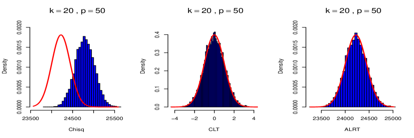
Figure S2: Histograms of $-2\rho\log\Lambda_{n}^{*}$ (Chisq), $(-2\log\Lambda_{n}^{*}-\mu_{n})/\sigma_{n}$ (CLT), and $Z_{n}$ (ALRT), where $n_{i}=100$, $1\leq i\leq k$, with $k=20$ and $p=5,20,50,95$.

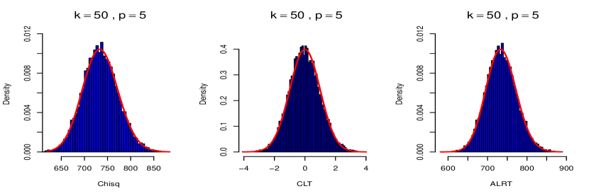
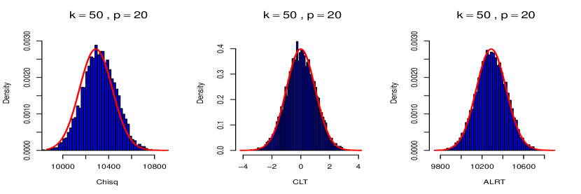
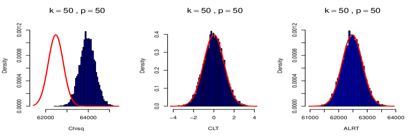
Figure S3: Histograms of $-2\rho\log\Lambda_{n}^{*}$ (Chisq), $(-2\log\Lambda_{n}^{*}-\mu_{n})/\sigma_{n}$ (CLT), and $Z_{n}$ (ALRT), where $n_{i}=100$, $1\leq i\leq k$, with $k=50$ and $p=5,20,50,95$.