Derivation of the First Passage Time Distribution for Markovian Process on Discrete Network

Abstract

Based on the analysis of probability flow, where the First Passage (FP) is realised as the sink of probability, we summarise the protocol to find the distribution of the First Passage Time (FTP). We also describe the corresponding formula for the discrete time case.

I Introduction

As the title shows, this note aims at providing with a concise résumé of the protocol and its derivation of the first passage time (FTP) distributions on the discrete Markov network whose transition rates are constant in time. While the well-written reviews and books on the derivation of the mean FPT are available for physicists [1, 2], the description of the probability distribution of the FTP [3] is not easily findable in the reviewed articles or books at least for the author. Nevertheless the FTP distribution is often useful when we analyse the transition network focusing on some specific states or transitions from which we extract, for example, the entropy production [4, 5].

The note originates from the course note of the author for the graduate course students. The contents may have been known among the experts of probability theory. Nevertheless, the note is presented here since the author had quite a few requests to bring it publicly accessible so that the users can cite it instead of explaining from scratch in their articles.

Below, after the definition of the problem and the introduction of the notations (§II), we derive the FTP distribution in the main part (§III). We also give a concrete example as an appendix A, which shows how the reduced master equation works. A completely parallel formalism is also given for the FTP distribution in the discrete time problem (§IV). The possibility of generalisation is discussed in §V.

II Master Equation and the First Passage Time (FTP) Problem

We recall the master equation on the discrete network and introduce some notations. Some problems are solvable much more easily by an ensemble approach, rather than focusing on individual realisations. The master equation is a basic tool for this approach.Those who are familiar to these notions may jump to the next section.

II.1 Master equation

Let us denote by $P_{\alpha}(t)$ the probability that the system is in the state $\alpha$ at time $t.$ We will use later the vector notation $\vec{P}(t)$ to represent the all components $\{P_{\alpha}(t)\}.$ Up to the precision of $\mathcal{O}(dt)$ the change of this probability is

$$P_{\alpha}(t+dt)-P_{\alpha}(t) =-{\left[{\sum_{\beta(\neq\alpha)}w_{\beta\leftarrow\alpha}dt}\right]}\,P_{\alpha}(t)$$ (2)

$$+\sum_{\beta(\neq\alpha)}{w_{\alpha\leftarrow\beta}dt\,P_{\beta}(t)}.$$

In dividing by $dt$ and rearranging the terms, it can be cast in the vector-matrix form of the master equation:

L 1

ddt

P_α(t)=∑_βM_α,βP_β(t), or

$$\frac{d}{dt}\vec{P}(t)={\sf M}\vec{P}(t),$$

where $M_{\alpha,\alpha}:=-\sum_{\gamma(\neq\alpha)}w_{\gamma\leftarrow\alpha}$ and $M_{\alpha,\beta}:=w_{\alpha\leftarrow\beta}$ for $\alpha\neq\beta.$ Then $\sf M$ is a square matrix. All the off-diagonal components are non-negative while the diagonal components are non-positive, such that $\sum_{\alpha}M_{\alpha,\beta}=0.$ We focus on the case where $\sf M$ is independent of time. Then the solution for the initial value problem reads $\vec{P}(t)=e^{{\sf M}t}\vec{P}(0).$

II.2 First-passage time (FPT) problem

At the initial time, $t=0,$ the system is put in the state $\alpha_{0}$. An individual realization allows to make jumps from a state to the other. When the system arrives for the first time at one of the “goal states” named $B=\{\beta_{i}\}$ the stochastic process stops. We denote by $B^{c}$ those states which are complement of $B.$ Our interests is in the statistics of the time and the last transition into $B$ at the first passage. We denote by ${\hat{\tau}}_{\tiny\rm FP}(\alpha_{0})$ this time of the first arrival. This is called the first passage time (FPT). This is a random variable. If $\alpha_{0}\in B,$ we define ${\hat{\tau}}_{\tiny\rm FP}(\alpha_{0})=0.$ Hereafter, we suppose that $\alpha_{0}\in B^{c}.$ In general it can happen that ${\hat{\tau}}_{\tiny\rm FP}(\alpha_{0})=\infty;$ when the network contains any “dead-end” state other than $B,$ the system’s state may remain in $B^{c}$ forever, see Fig. 1.

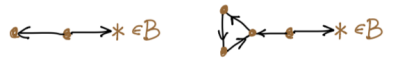
Figure 1: The cases where ${\hat{\tau}}_{\tiny\rm FP}(\alpha_{0})=\infty$ can happen. We exclude such cases from our consideration.

Hereafter, we exclude such cases; we assume that from any state (node) $\alpha_{0}$ in $B^{c}$ the system can eventually reach one of the $B$ states.

III Derivation of the FTP distribution

III.1 Basic idea

In the ensemble-based view, the master equation can be interpreted so that a unit “mass” (in fact the probability being 1) is injected at the node $\alpha_{0}$ at $t=0,$ and then the injected mass (probability) flows out through the links at the rate being the transition rate.

For the purpose of analysing the FTP we modify the network such that any state belonging to $B$ is replaced by a sink (“black hole (of mass)”), where no outward transition occurs, see Fig. 2.

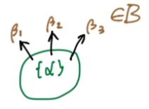
Figure 2: The arrows show the one-way exits to the goal sites, $\{\beta_{1},\beta_{2},\beta_{3}\}\subset B,$ from the group of states, $\{\alpha\}=B^{c},$ which are represented by a circle.

Then the probability $Prob({\hat{\tau}}(\alpha_{0})\in[t,t+dt])$ is given by the cumulated flow of the mass (probability) $B^{c}\to B$ during this time interval. When the states are indexed by continuous parameters such as Euclidean coordinates, $B$ is usually represented as absorbing boundaries. All what remains to do is the formulation of this idea as a recipe.

III.2 Basic recipe

Let us begin by an extremely simple network of which $B^{c}=\{1\}$ and $B=\{*\}$. The general case can be formulated later by using the analogy to this case. The only reactions here are $1{\longleftrightarrow}*$, with the rates, $w$ for $1\rightarrow*$ and $w^{\prime}$ for $1\leftarrow*,$ respectively.

1. Among the normalized probabilities, $P_{1}$ and $P_{*},$ we exclude $P_{*},$ and omit the transition ($w^{\prime}$) emitted from $*$.
   Then we solve only $\frac{d}{dt}{P}_{1}(t)=-{\frac{1}{\tau}}{P}_{1}(t)$ from $P_{1}(0)=1.$ We find $P_{1}(t)=P_{1}(0)e^{-t/\tau}.$

2. We understand that

   $$Prob\big{(}\mbox{\small``the transition $1\to*$ takes place in the interval $[t,t+dt[$\,''}\big{)}$$ (4)

   $$=P_{1}(t)-P_{1}(t+dt)\simeq-\frac{dP_{1}(t)}{dt}\,dt.$$

   Therefore, $-\frac{dP_{1}(t)}{dt}$ is the probability density for the FPT to be $t$. If we want to know $Prob\big{(}\mbox{``FPT is less than $t$''}),$ we can integrate; $\int_{0}^{t}(-\frac{dP_{1}(t^{\prime})}{dt^{\prime}})dt^{\prime}=-P_{1}(t)+P_{1}(0)=1-P_{1}(t).$ It is intuitively correct because $P_{1}(t)=Prob\big{(}\mbox{``FPT is more than $t$''})$ in the present case.

III.3 Extended recipe

We study the network allowing more than one inner states ($\in B^{c}$) and goal states ($\in B$).

Step 1. Reduced transition network

We remove from the full transition network all the transition edges from the group $B.$ — We do this so that the process is over once the system reach the “black hole” $B$-states. These $B$-states then become just a sink, having only in-coming edges. As a consequence $P_{\beta}$’s with $\beta\in B$ appear no more.

We call the resulting network the reduced transition network.

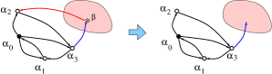
Figure 3: (Left) Original transition network including $B=\{\beta\}.$ (Right) Reduced network.

Fig. 3 illustrates the construction of the reduced transition network.

As the master equation, we are left with a reduced master equation,

$$\frac{d}{dt}\vec{P}^{*}(t)={\sf M}^{*}\vec{P}^{*}(t),$$

where $\vec{P}^{*}(t)$ is the vector $\vec{P}(t)$ less the states in $B$-group, and the reduced matrix ${\sf M^{*}}$ is again square.

The set of master equations for the original (i.e., non-reduced) network contains the equations $\frac{dP_{\beta}}{dt}=\ldots$ with $\beta\in B.$ In the reduced network, those equations are absent. The solution of the reduced master equation can be written as $\vec{P}^{*}(t)=e^{{\sf M}^{*}t}\vec{P}^{*}(0).$ If the initial state is $\alpha_{0}$ we write $\vec{P}^{*}(0)=|\alpha_{0}\rangle.$ Comparing with the equations in § III.2, we see how the basic scheme has been extended.

  Numerically, $e^{{\sf M}^{*}t}$ is calculated using the spectral decomposition, ${\sf M}^{*}=\sum_{\nu}|\lambda_{\nu}\rangle\lambda_{\nu}\langle\lambda_{\nu}|$, that is, $e^{{\sf M}^{*}t}=\sum_{\nu}|\lambda_{\nu}\rangle e^{\lambda_{\nu}t}\langle\lambda_{\nu}|.$ Once $e^{{\sf M}^{*}t}$ is obtained, $\vec{P}^{*}(t)$ is given by the matrix-vector product, $\vec{P}^{*}(t)=e^{{\sf M}^{*}t}\vec{P}^{*}(0)=e^{{\sf M}^{*}t}|\alpha_{0}\rangle.$

Remarks:
(i) The matrix ${\sf M}$ or ${\sf M}^{*}$ can have complex eigenvalues. Nevertheless, when ${\sf M}$ or $e^{{\sf M}t}$ are applied to a physically meaningful $\vec{P}^{*},$ the result is always physically meaningful.
(ii) Having excluded the diverging FPT, all the eigenvalues of ${\sf M}^{*}$ must have strictly negative real part because $\vec{P}^{*}(t)$ with any initial $\alpha_{0}$ should decay to the reduced zero-vector, $\vec{0}^{*},$ for $t\to\infty.$
(iii) The evolution of $\vec{P}^{*}(t)$ is generally different from the $B^{c}$-part of the full evolution, $\vec{P}(t),$ because the former excludes the “returning from $B$-group.”

Step 2. Probability distribution of FPT

In order to simplify the notation, we introduce a special row vector, à la Dirac, in the reduced state space, $\langle\,|$ whose $\alpha(\in{B^{c}})$ components are all unity (=1). With $\langle\,|$ we have the short hand like $\sum_{\alpha\in B^{c}}P^{*}_{\alpha}=\langle\,|\vec{P}^{*}\rangle,$ or $\sum_{\alpha\in B^{c}}{M}^{*}_{\alpha,\mu}=\langle\,|{\sf M}^{*}|\mu\rangle.$

$\langle\,|\vec{P}^{*}(t)\rangle$ is the probability that the system has not reached any goal state at time $t.$ Then probability that the system reaches for the first time one of the $B$ states in the interval $[t,t+dt[$ reads, in analogy to (4),

$$Prob{\left({\hat{\tau}_{\tiny\rm FP}(\alpha_{0})\in[t,t+dt[}\right)} = \langle\,|\vec{P}^{*}(t)\rangle-\langle\,|\vec{P}^{*}(t+dt)\rangle$$ (5)

$$= -\langle\,|\frac{d\vec{P}^{*}(t)}{dt}\rangle\,dt$$ (6)

$$= -\langle\,|{\sf M}^{*}|\vec{P}^{*}(t)\rangle\,dt.$$ (7)

The probability density of FTP is, therefore, the coefficient of $dt$ on the right extreme part :

$$p_{FPT}(t)=-\langle\,|{\sf M}^{*}|\vec{P}^{*}(t)\rangle$$

The normalisation is ${\int^{+\infty}_{0}}p_{FPT}(t)dt=1.$
  Numerically: As we already have $|\vec{P}^{*}(t)\rangle,$ the further matrix-vector product with $(-\langle\,|{\sf M}^{*})$ from the left gives $p_{FTP}(t).$

Theoretically : We can rewrite the r.h.s. of (5) to represent:

$$Prob{\left({\hat{\tau}_{\tiny\rm FP}(\alpha_{0})\in[t,t+dt]}\right)}=\sum_{\beta\in B}\sum_{\alpha\in B^{c}}w_{\beta\leftarrow\alpha}P_{\alpha}^{*}(t)dt,$$ (8)

where only those $\alpha\in B^{c}$ that have non-zero rate $w_{\beta\leftarrow\alpha}$ to any goal state $\in B$ contribute. (Note that $w_{\beta_{i}\leftarrow\alpha}$ is not an element of ${\sf M}^{*}.$) — We propose two versions of intuitive explanation of (8).
(Version1) The surviving probability, $\langle\,|P^{*}(t)\rangle,$ decays only through the transitions $w_{\beta\leftarrow\alpha}$ ($\beta\in B,\alpha\in B^{c}$). We, therefore, measure the escaping flux of probability through those channels.
(Version 2) The reduced master equation has the divergence form, $d|P^{*}\rangle/dt=-\nabla\cdot J.$ Then its “volume integral” $\langle\,|$ can be rewritten by the “Gauss’ divergence theorem,” $\int_{V}dV(\nabla\cdot J)=\oint_{\partial V}d\vec{S}\cdot J.$ Thus $-\frac{d\langle\,|P^{*}\rangle}{dt}=\oint_{\partial V}d\vec{S}\cdot J$ is found. Lastly the $J$ on the boundary $\partial V$ is the “fluxes to $B$” through $w_{\beta\leftarrow\alpha}$ ($\beta\in B,\alpha\in B^{c}$).

III.4 Outcomes of FTP distribution

III.4.1 Mean FPT (MFPT)

Often we focus on the mean FTP. By definition,

$$E[\hat{\tau}_{\tiny\rm FP}|\alpha_{0}]=\int_{0}^{\infty}t\,Prob{\left({\hat{\tau}_{\tiny\rm FP}(\alpha_{0})\in[t,t+dt]}\right)}.$$

Using (5) and the integration by parts w.r.t. time $t$, we have

$$E[\hat{\tau}_{\tiny\rm FP}|\alpha_{0}] = \int_{0}^{\infty}t\,{\left({-\langle\,|\frac{d\vec{P}^{*}(t)}{dt}\rangle}\right)}\,dt$$ (9)

$$= \int_{0}^{\infty}\langle\,|P^{*}(t)\rangle dt=\langle\,|{\left({-{\frac{1}{{\sf M}^{*}}}}\right)}|\alpha_{0}\rangle.$$ (10)

To have the last equality, we used $|P^{*}(t)\rangle=e^{{\sf M}^{*}t}|\alpha_{0}\rangle.$ Many books for physicists mentions only the MFPT, because the calculation of MFPT does not require the FTP distribution. As we have seen, however, the FPT distribution is simpler and more basic.

  Numerically: The r.h.s. of the MFPT expression requires the calculation of the inverse of ${\sf M}^{*}.$ A usual protocol, instead, is to multiply by $M^{*}_{\alpha_{0},\alpha}$ and take the sum over $\alpha_{0}$ over the reduced network states. Then we have

$$\sum_{\alpha_{0}}E[{\hat{\tau}}|\alpha_{0}]\,M^{*}_{\alpha_{0},\alpha} = -\sum_{\alpha^{\prime}}\sum_{\alpha_{0}}({\frac{1}{{\sf M}^{*}}})_{\alpha^{\prime},\alpha_{0}}M^{*}_{\alpha_{0},\alpha}$$ (11)

$$= -\sum_{\alpha^{\prime}}\delta_{\alpha^{\prime},\alpha}$$ (12)

$$= -1\qquad\mbox{for $\forall\alpha.$}$$ (13)

By using the solver of coupled linear equations we find $E[{\hat{\tau}}|\alpha_{0}]$ for $\forall\alpha_{0}$.

III.4.2 Exit problem

Sometimes we are not interested in the value of FPT, but rather interested in how it finished. That is, among the goal states $B$, we ask which $\beta$ has absorbed the state point. See Fig. 2. For this purpose, we segregate the result (8). If we like to know the probability that the state finish in $\beta_{i}(\in B),$ we calculate the partial probability:

$$\frac{Prob{\left({\mbox{exit to $\beta_{i}$}|\alpha_{0}}\right)}}{Prob{\left({\mbox{exit to $B$}|\alpha_{0}}\right)}} = {\int_{0}^{\infty}\sum_{\alpha\in{B^{c}}}w_{\beta_{i}\leftarrow\alpha}P_{\alpha}^{*}(t)dt}$$ (14)

$$= {\sum_{\alpha\in{B^{c}}}w_{\beta_{i}\leftarrow\alpha}\langle\alpha|{\left({-{\frac{1}{{\sf M}^{*}}}}\right)}|\alpha_{0}\rangle},$$ (15)

where we have noticed our setup, $Prob{\left({\mbox{exit to $B$}|\alpha_{0}}\right)}=1$ . As noticed above $w_{\beta_{i}\leftarrow\alpha}$ is not an element of ${\sf M}^{*}.$

The exit problem plays an important role in the evolution, namely the fixation of a new genotype among the (finite) population. Either the extinction of the new ( and overwhelmingly neutral) genotypes or the extinction of the original one are the two exits.

IV Discrete time version

”Master equation”

: We denote by $n\in{\mathbb{N}}_{0}$ the discrete time and $\vec{P}(n)$ denotes the probability vector of the original (non-reduced) network. The evolution of $\vec{P}(n)$ writes

$$\vec{P}(n+1)={\sf K}\vec{P}(n);$$

where the transfer matrix ${\sf K}$ is supposed to be constant in time. The normalization of the probability imposes $\langle\,|{\sf K}=\langle\,|,$ or $\sum_{j}K_{j\leftarrow i}=1$ for $\forall i.$ Again we suppose the case when any states in $B^{c}$ can eventually reach one of the $B$ states.

First Passage Time

: When the initial state $\alpha_{0}$ is already in $B$ block, we define that FTP is zero. For $\alpha_{0}\in B^{c}$ the FPT, $\hat{\tau}_{FP}(\alpha_{0}),$ should be positive. It is, therefore, consistent to say ${\hat{\tau}}_{FP}(\alpha_{0})=1$ if the system enters $B$ at $t=1.$ In general we say ${\hat{\tau}}_{FP}(\alpha_{0})=n$ if the system enters $B$ at $t=n$ but have remained in $B^{c}$ for $0\leq t<n.$

“Reduced transfer matrix”

: We introduce the state space that contains only the states belonging to $B^{c},$ and also introduce the reduced transfer matrix ${\sf K}^{*}$ that lacks the rows and lines corresponding to $B$ states. Recall that the element $K_{\beta\leftarrow\alpha}$ with $\alpha\in B^{c}$ and $\beta\in B$ is contained in ${\sf K}^{*}$ in the form, $K_{\alpha\leftarrow\alpha}=1-\sum_{\beta\in B}K_{\beta\leftarrow\alpha}.$

Results

: Because the basic idea is the same as the case of continuous time, we only write some resultant formulas. We shall denote by $S_{n}$ the state of the system at time $n(\geq 0).$ We suppose that $\alpha_{0}\in B^{c}.$ :
i) Cumulated probability of FPT for $n\geq 0$:

$$Prob({\hat{\tau}}_{FP}>n|S_{n=0}=\alpha_{0})=\langle\,|({\sf K}^{*})^{n}|\alpha_{0}\rangle.$$ (17)

Especially $Prob({\hat{\tau}}_{FP}>0|S_{n=0}=\alpha_{0})=1.$

ii) Probability of FPT being $n$:
In our setup, $Prob({\hat{\tau}}_{FP}=0|S_{n=0}=\alpha_{0})=0,$ and for $n\geq 1$

$$Prob({\hat{\tau}}_{FP}=n|S_{n=0}=\alpha_{0})$$ (18)

$$=Prob({\hat{\tau}}_{FP}>\!n-1|S_{n=0}=\alpha_{0})\!-\!Prob({\hat{\tau}}_{FP}>\!n|S_{n=0}=\alpha_{0})$$ (19)

$$=\langle\,|({\bf 1}-{\sf K}^{*})({\sf K}^{*})^{n-1}|\alpha_{0}\rangle.$$ (20)

Using $\langle\,|\alpha_{0}\rangle=1$ and $({\sf K}^{*})^{\infty}={\sf 0}$ the normalisation reads

$$\sum_{n=1}^{\infty}Prob({\hat{\tau}}_{FP}=n|S_{n=0}=\alpha_{0})=\langle\,|\alpha_{0}\rangle-\langle\,|({\sf K}^{*})^{\infty}|\alpha_{0}\rangle=1,$$ (21)

iii) Probability of FPT with specified route from $\alpha_{s}\in B^{c}$ to $\beta_{s}\in B.$:

$$Prob({\hat{\tau}}_{FP}=n\wedge\mbox{(through $\beta_{s}\leftarrow\alpha_{s}$)}|S_{n=0}=\alpha_{0})$$ (22)

$$={\sf K}_{\beta_{s}\leftarrow\alpha_{s}}\langle\alpha_{s}|({\sf K}^{*})^{n-1}|\alpha_{0}\rangle,$$ (23)

because $\langle\alpha_{s}|({\sf K}^{*})^{n-1}|\alpha_{0}\rangle$ gives the probability of finding the system in $\alpha_{s}$ after $(n-1)$ steps then we multiply the conditional probability of the specific exit, ${\sf K}_{\beta_{s}\leftarrow\alpha_{s}}.$ (Note that “${\sf K}^{*}_{\beta_{s}\leftarrow\alpha_{s}}$” does not exist.) The normalisation should be such that

$$\sum_{\beta_{s}\in B}\sum_{\alpha_{c}\in B^{c}}Prob({\hat{\tau}}_{FP}=n\wedge\mbox{(through $\beta_{s}\leftarrow\alpha_{s}$)}|S_{n=0}=\alpha_{0})$$ (24)

$$=Prob({\hat{\tau}}_{FP}=n|S_{n=0}=\alpha_{0}).$$ (25)

V Concluding discussion

Based on the analysis of probability flow, where the FPT is realised as the sink of probability, we have summarised the protocol to construct the FPT distribution. Key is to reform the transition network in the way that the goal states are made to be the sink, even valid for non-Markovian case. The reduced transition rate matrix ${\sf M^{*}}$ is a partial diagonal block of the original one, ${\sf M},$ in the simple cases that are treated in the main text. However, we don’t stress this view “reduced” too much because the idea of absorbing nodes (sinks) is more generally applicable; we can sometimes add nodes or replicate the original network so as to adapt to more advanced FP problem. For example, we can replace the particular links $\alpha_{1}\stackrel{{\scriptstyle M_{12}}}{{\to}}\alpha_{2}$ and $\alpha_{2}\stackrel{{\scriptstyle M_{21}}}{{\to}}\alpha_{1}$ in a network by $\alpha_{1}\stackrel{{\scriptstyle M_{12}}}{{\to}}*$ and $\alpha_{2}\stackrel{{\scriptstyle M_{21}}}{{\to}}*,$ respectively, where $*\in B$ is the added absorbing node. In the ring network [20] depicted by Fig.4(a), Figs.4(b), 4(c) and 4(d) implement, respectively, (b) the counter of the number of $D\to A$ transitions ($D\to A^{\prime}$ giving the first one), (c) the competition of the earlier passage of $D\to C$ vs $C\to D,$ and (d) the first consecutive transitions $C\to D\to A.$

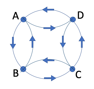
(a)

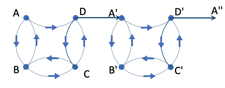
(b)

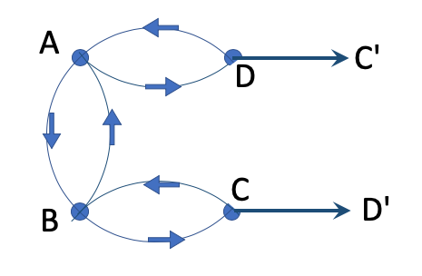
(c)

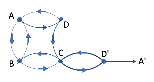
(d)

Figure 4: See the main text.

Moreover, if we extend the idea of replicating the nodes, we can Markovianize exactly some non-Markovian model having a two neighbors (Fig.5(a)$\to$(b)) or three neighbors (Fig.5(c)$\to$(d)). In both cases the node memories from where it came.

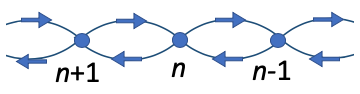
(a)

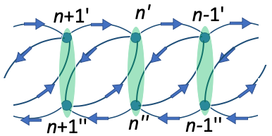
(b)

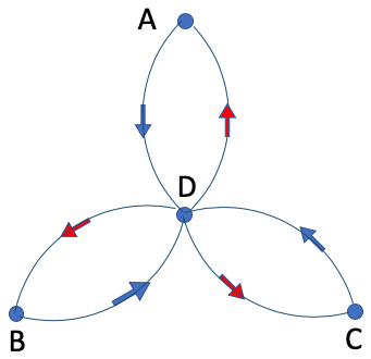
(c)

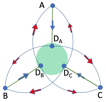
(d)

Figure 5: See the main text.

Appendix A A paradoxical example of MFPT

We apply the present approach for the continuous time to find a MFPT of a particular example which is somehow counter-intuitive, the situation being related to so called waiting-time paradox.

Let us consider a circular transition network with unique exit like Fig. 6. The network is a loop with $n$ nodes complemented by a unique exit from “$1$” to “$b$”. The uni-directional transition rate on the loop is uniform (rate $w$) and the transition rate to the exit is $w^{*}$. Starting at $t=0$ from the state “$\alpha_{0}$” among “1” to “$n$”, we like to know the expectation value of the FPT ($E[\hat{\tau}_{\tiny\rm FP}|\alpha_{0}]$), which we denote by $\tau_{MFP}(\alpha_{0}).$

Figure 6: The circular transition network with an exit.

Solving for MFPT

1. We write down the master equation for $p_{1},\ldots,p_{n},$ in the form like $dp_{j}(t)/dt=\ldots$ with $1\leq j\leq n.$ Then from this equation, find the reduced matrix ${\sf M}^{*}$. This matrix reads (The diagonal elements are negative.)

Surprisingly the result is independent of $w$. We like to discuss qualitatively the result in the two extreme cases, i.e., $w^{*}/w\ll 1$ and $w^{*}/w\gg 1.$

For $w^{*}/w\ll 1$:

We can find $\tau_{MFP}(1)$ approximately as follows. Because of the relatively high transition rate along the loop, the mean time for an entire circulation, $\frac{n}{w}$, is much shorter than the waiting time from “1” to “b”, ${\frac{1}{w^{*}}}.$ Therefore, the probability is almost evenly shared among the $n$ states along the loop, that is, $P_{1}\simeq\cdots\simeq P_{n}\simeq\frac{P_{loop}(t)}{n},$ where $P_{loop}(t)$ is the total probability on the loop (i.e. in the group $B^{c}$). From such quasi-steady state, the probability flows out slowly to “b”. The decay of $P_{loop}(t)$ reads $\frac{d}{dt}P_{loop}(t)=-w^{*}P_{1}(t)=-w^{*}\frac{P_{loop}(t)}{n}.$ We then have $P_{loop}(t)=e^{-\frac{w^{*}}{n}t}.$ Since the probability density of FPT is $-\frac{d}{dt}P_{loop}(t)=\frac{w^{*}}{n}P_{loop}(t),$ we find $E[\hat{\tau}_{\tiny\rm FP}|\mbox{``1''}]={\frac{n}{w^{*}}}.$

For $w^{*}/w\gg 1$

We can find $\tau_{MFP}(1)$ approximately as follows. In most cases, the system will exit directly, after the time $\sim 1/w^{*}$. The probability for such case is $w^{*}/(w+w^{*})=1-\mathcal{O}(\frac{w}{w^{*}}).$ However, in rare case with the probability, $w/(w+w^{*})\simeq\frac{w}{w^{*}},$ the system jumps to “2” instead of “b”. Let us denote by $\Delta t_{1\to 2}$ the time took from “1” to “2” . Once the system finds in “2”, we should count time $\sim\frac{n-1}{w}$ until it returns to “1”. Now if we count these two cases, the mean FP time is estimated to be

$$E[\hat{\tau}_{\tiny\rm FP}|\mbox{``1''}]$$ (29)

$$=[1-\mathcal{O}(\frac{w}{w^{*}})]\frac{1}{w^{*}}+\frac{w}{w^{*}}{\left({\Delta t_{1\to 2}+\frac{n-1}{w}}\right)}$$ (30)

$$={\frac{n}{w^{*}}}+\frac{w}{w^{*}}\Delta t_{1\to 2}.$$ (31)

The last point is the estimation of $\Delta t_{1\to 2}.$ If it were estimated to be $\simeq{\frac{1}{w}}$, we would have a wrong result, $\frac{n+1}{w^{*}}.$ The correct estimation of $\Delta t_{1\to 2}$ is $\frac{1}{w+w^{*}}\underline{\simeq{\frac{1}{w^{*}}}}.$ This issue is related to the known paradox as explained below:

Waiting-time paradox

: Suppose a network given by $2\stackrel{{\scriptstyle w}}{{\longleftarrow}}1\stackrel{{\scriptstyle w^{*}}}{{\longrightarrow}}b$ and start by “1” at $t$ = $0.$ If we solve the full master equations for $(P_{1},P_{2},P_{b})^{t},$ we will have

$${\left({\begin{matrix}P_{1}(t)\\ P_{2}(t)\\ P_{b}(t)\\ \end{matrix}}\right)}={\left({\begin{matrix}e^{-(w+w^{*})t}\\ \frac{w}{w+w^{*}}[1-e^{-(w+w^{*})t}]\\ \frac{w^{*}}{w+w^{*}}[1-e^{-(w+w^{*})t}]\\ \end{matrix}}\right)}$$ (32)

Noting that $P_{2}(t)$ is the joint probability, $Prob(\hat{\tau}_{1\to 2}<t\,\wedge\,1\to 2),$ on the one hand, and that the exit probability to $2$ is $Prob(1\to 2)=P_{2}(\infty)=\frac{w}{w+w^{*}}$ on the other hand, we have

$$Prob(\hat{\tau}_{1\to 2}<t\,|\,1\to 2)$$ (33)

$$=\frac{Prob(\hat{\tau}_{1\to 2}<t\,\wedge\,1\to 2)}{Prob(1\to 2)}$$ (34)

$$=1-e^{-(w+w^{*})t}$$ (35)

Therefore, when the transition $1\to 2$ takes place, it occurs in $[t,t+dt[$ at the probability, $\frac{d(1-e^{-(w+w^{*})t})}{dt}dt=(w+w^{*})e^{-(w+w^{*})t}dt.$ In conclusion, when the transition $1\stackrel{{\scriptstyle w}}{{\to}}2$ competes with $1\stackrel{{\scriptstyle w^{*}}}{{\to}}b,$ the mean waiting time of $1\to 2$ transition is shortened to ${\frac{1}{w+w^{*}}}\simeq{\frac{1}{w^{*}}}$ from ${\frac{1}{w}}$ of the non-competing case.

References

- Hänggi et al. [1990] P. Hänggi, P. Talkner, and M. Borkovec, Rev. Mod. Phys. 62, 251 (1990).
- Redner [2001] S. Redner, A Guide to First-Passage Processes (Cambridge University Press, 2001).
- Haake et al. [1981] F. Haake, J. W. Haus, and R. Glauber, Phys. Rev. A 23, 3255 (1981).
- Manzano et al. [2019] G. Manzano, R. Fazio, and E. Roldán, Phys. Rev. Lett. 122, 220602 (2019).
- Neri [2020] I. Neri, Phys. Rev. Lett. 124, 040601 (2020).
- Note [1] The exponential of a matrix is defined by .
- Note [2] The extension to the probabilistic initial condition is straightforward.
- Note [3] In the network language, the transition from node to node on the network end once the state jumps to one of the nodes belonging to .
- Note [4] When a more precision is required, we define that the is such that the system is found in through but in for .
- Note [5] One can say that, if we write the original equations as then the reduced matrix contains only the block .
- Note [6] The eigenvector and its conjugate, have generally different components but can be made so that is assured. More can be learned, check under the key word polar decomposition (of square matrix).
- Note [7] Cf. The non-reduced must have at least a zero eigenvalue.
- Note [8] More precisely we should write or etc. for the reduced network. We will, however, omit ∗ whenever it is clear.
- Note [9] Cf. In the non-reduced network .
- Note [10] is invertible. cf. has zero eigenvalue and therefore non-invertible.
- Note [11] In the vector-matrix sense, we multiply each side of the vector equation (9) the transposed matrix, from the left. (Attention: is not the transpose of ).
- Note [12] When i.e., in the presence of internal trapping, we should divide the second and the last expressions, respectively, by this quantity, i.e. .
- Note [13] As was discussed in the footnote [10], if we divide into four blocks symbolically, the reduced one is the square block.
- Note [14] By contrast the elements like with and appear only in the blocks and .
- Harunari et al. [2022] P. E. Harunari, A. Dutta, M. Polettini, and Édgar. Roldán, What to learn from few visible transitions’ statistics? (https://arxiv.org/abs/2203.07427) (2022).
- Note [15] The details: By adding the middle equations we find Next, substituting this into the first equation, we have Finally, substituting this into the last equation, we have .
- Note [16] This case is more subtle. A simple-minded argument could gave approximately.