Classical Pendulum Clocks Break the Thermodynamic Uncertainty Relation

Abstract

The thermodynamic uncertainty relation expresses a seemingly universal trade-off between the cost for driving an autonomous system and precision in any output observable. It has so far been proven for discrete systems and for overdamped Brownian motion. Its validity for the more general class of underdamped Brownian motion, where inertia is relevant, was conjectured based on numerical evidence. We now disprove this conjecture by constructing a counterexample. Its design is inspired by a classical pendulum clock, which uses an escapement to couple the motion of an oscillator to another degree of freedom (a “hand”) driven by an external force. Considering a thermodynamically consistent, discrete model for an escapement mechanism, we first show that the oscillations of an underdamped harmonic oscillator in thermal equilibrium are sufficient to break the thermodynamic uncertainty relation. We then show that this is also the case in simulations of a fully continuous underdamped system with a potential landscape that mimics an escaped pendulum.

Introduction.

Being able to tell the time precisely, regardless of astronomical observation, has ample importance for virtually all of human civilisation. Ancient water clocks or hour glasses relied on the steady flow of matter. However, the precision of such devices was strongly limited, because of inhomogeneities or unpredictable external influences. A revolution in the history of timekeeping was the invention of the escapement. This mechanism uses coherent oscillations of a physical system to regulate the forward motion of a cog loaded with a weight and connected to a hand that displays time. Galileo realised that a swinging pendulum can provide such oscillations, since its period is (for small angles) independent of its amplitude. This inspired Huygens’ invention of the pendulum clock in 1656, setting standards in precision for centuries to come Marrison (1948). This Letter shows that this well-established principle even allows for precision beyond the thermodynamic limits that have so far been believed to apply to classical systems.

The performance of a clock can be quantified by its precision and its turnover of energy. These quantities take center stage in the thermodynamic uncertainty relation (TUR) Horowitz and Gingrich (2020), formulated originally for biomolecular systems Barato and Seifert (2015). It describes a trade-off between the overall cost for driving a system and the precision observed in any output current.

More specifically, we consider a Markovian system in a steady state producing an integrated current $Y(t)$ (e.g., the accumulated angle of a clock hand). The energetic cost of driving is quantified by the entropy production rate $\sigma$. It corresponds (in the absence of chemical changes) to the heat dissipated into a surrounding heat bath, divided by its constant temperature $T$. This heat needs to be equal to the energy expended on the system’s driving. The TUR states that

$$\frac{\mathrm{Var}\,{Y(t)}}{\left\langle Y(t)\right\rangle^{2}}t\sigma\geq 2,$$ (1)

where we set Boltzmann’s constant $k_{B}=1$ and define $\mathrm{Var}\,{Y(t)}\equiv\left\langle Y(t)^{2}\right\rangle-\left\langle Y(t)\right\rangle^{2}$, with averages $\left\langle\ldots\right\rangle$ taken in the steady state. This relation was first proven for the limit of large times $t$ Gingrich et al. (2016), and later generalised to finite times Pietzonka et al. (2017); Horowitz and Gingrich (2017).

The TUR rests on the premise of local detailed balance, relating the log-ratio of forward and backward transition rates between discrete states of a system to the entropy produced in a transition Seifert (2018). Brownian diffusion fits into this framework if it can be described as overdamped, meaning that momentum variables are assumed to relax instantly to a local equilibrium. Here, the TUR is recovered either through a fine discretisation of the state space or directly from a Langevin description Dechant and Sasa (2018a, b).

An underdamped description of Brownian dynamics explicitly retains the inertia that is present in every classical dynamical system. Yet, this more general dynamics lies beyond the original framework of the TUR. There, transitions in a finely discretised phase space appear irreversible without the simultaneous reversal of momenta, which leads to a formally divergent entropy production, despite the actual entropy production being finite Fischer et al. (2018). Bounds on the precision of irreversible currents in underdamped systems have been derived Fischer et al. (2018); Van Vu and Hasegawa (2019); Lee et al. (2019); Vo et al. (2020); Lee et al. (2021), however, they are weaker than the TUR or require additional information about the system (beyond the entropy production rate). Violations of the TUR in its original form have been observed where an external magnetic field breaks time-reversal symmetry Brandner et al. (2018); Chun et al. (2019). It is also known that ballistic motion on short timescales spoils the finite-time variant of the TUR. Yet, numerical evidence suggested that the TUR would hold for large times Fischer et al. (2020), in line with the intuition that sufficient driving is needed to overcome the time-reversal symmetry of thermal equilibrium.

In this Letter, we provide a disproof of the TUR for underdamped dynamics. As it turns out, the principle of an escapement, originally conceived to ward off environmental perturbations, is effective even if these are of purely thermal origin. We develop a minimal thermodynamically consistent model for a pendulum clock, which yields at given energetic cost high precision beyond the limits of the TUR.

Once wound, pendulum clocks operate autonomously. Hence they are different from periodically driven systems, for which refined TUR’s have been derived Barato and Seifert (2016); Proesmans and Van den Broeck (2017); Koyuk et al. (2019); Barato et al. (2018); Koyuk and Seifert (2020). Taken for themselves, periodic systems do not obey the original TUR. It nonetheless holds on a global scale taking into account the infinite cost required to generate a deterministic protocol in a Markovian framework Barato and Seifert (2017). We take this idea further, describing an escapement as a way to couple a discrete system to an oscillating system that is not perfectly precise, but comes at small (or even zero) energetic cost.

General setting.

We consider a system consisting of two subsystems, as shown in Fig. 1. The first, which we call an “oscillator,” could be an arbitrary physical system described by a state $x(t)$ (in our main example and Fig. 1 we choose this to be a pendulum subject to thermal noise). The other subsystem, which we call a “counter,” is a one-dimensional degree of freedom on an infinite discrete lattice. For notational convenience we label pairs of adjacent states by integers $y$, denoting the upper state as $y^{-}$ and the lower state as $y^{+}$, and identifying $y^{+}$ and $(y+1)^{-}$ as the same states of the counter. In the picture of a pendulum clock, the discrete state space of the counter corresponds to orientations of the seconds hand, mapped to the infinite number line by keeping account of full revolutions around the clock face.

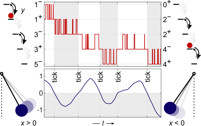
Figure 1: Minimal model for a pendulum clock subject to thermal noise. An oscillating degree of freedom $x$ (bottom), is coupled to a discrete counter degree of freedom (top), where $y$ labels pairs of adjacent states $y^{-}$ and $y^{+}$. A typical trajectory is shown in the middle, with snapshots of the configuration at its beginning (left) and end (right). Transitions of the counter are generally biased downward. When $x>0$, transitions between even pairs of states $y^{\pm}$ are strongly suppressed and transitions between odd ones are very fast, and vice versa for $x<0$. This way, transitions from one pair of states $y$ to a neighbouring one are possible only upon a “tick,” when the pendulum crosses through $x=0$.

Jumps between any $y^{-}$ and the corresponding $y^{+}$ occur continuously in time and are biased toward the latter by a nonconservative force (e.g., provided by a weight on a cord). The work delivered by this force in a forward jump divided by the temperature $T$ defines the affinity $A$, fixing the log-ratio of the rates for forward and backward transitions through the local detailed balance condition

$$\ln\frac{k(y^{-}\to y^{+})}{k(y^{+}\to y^{-})}=A.$$ (2)

Since the states $y^{-}$ and $y^{+}$ have the same internal energy, the first law requires the work to be dissipated as heat, increasing the entropy in the environment by $A$. Conversely, a backward step decreases this entropy by $A$.

The escapement mechanism is realised by exploiting the freedom of choice of a common prefactor to both rates, which can be made dependent on the state $x$ of the oscillator. We model that the escapement can be in either of two states $i(x)\in\{0,1\}$. If $x$ is the angular displacement of a pendulum, an obvious choice is $i(x)=1$ for $x\geq 0$ and $i(x)=0$ for $x<0$. For $i(x)=1$, we set the transition rates $k(y^{\mp}\to y^{\pm})=k^{\pm}$ for $y$ odd and $k(y^{\mp}\to y^{\pm})=\varepsilon k^{\pm}$ for $y$ even. Vice versa, for $i(x)=0$, we set $k(y^{\mp}\to y^{\pm})=\varepsilon k^{\pm}$ for $y$ odd and $k(y^{\mp}\to y^{\pm})=k^{\pm}$ for $y$ even. The rates $k^{+}$ and $k^{-}=k^{+}\exp(-A)$ are both chosen to be much larger than the inverse of the fastest relevant timescale of the oscillator. In contrast, the factor $\varepsilon>0$ is chosen sufficiently small such that the rates $\varepsilon k^{\pm}$ are much smaller than the inverse of the slowest timescale of the oscillator. This choice of rates ensures that, after a change of the state $i(x)$, the counter is effectively constrained to a single pair of states $y^{\pm}$, between which it equilibrates quickly. It can then be found in either of the states at the conditional probability

$$p_{\pm}=k^{\pm}/(k^{+}+k^{-})=\exp(\pm A/2)/[2\cosh(A/2)].$$ (3)

Next time the state $i(x)$ changes, the counter will have ended up in either of the states $y^{\pm}$, whose link then gets effectively broken. Depending on this outcome, the counter then proceeds to fluctuate either between states $(y-1)^{\pm}$ or $(y+1)^{\pm}$.

We see that upon every change of $i(x)$, called a “tick” in the following, the variable $y$, labeling the pair of states between which the counter currently fluctuates, performs a single step of an asymmetric random walk. In this random walk, the number of ticks $N(t)$ up to time $t$ plays the role of a discrete time. The steps taken by $y$ upon subsequent ticks are independent and identically distributed, such that (given $y=0$ at time $t=0$) the central limit theorem yields the conditional probability $p(y|N)$ as a Gaussian with mean and variance

$$NJ_{y|N} \equiv N(p^{+}-p^{-})=N\tanh(A/2),$$ (4)

$$2ND_{y|N} \equiv N[p^{+}+p^{-}-(p^{+}-p^{-})^{2}]=N/\cosh^{2}(A/2).$$ (5)

While the dynamics of the counter depends strongly on the dynamics of the oscillator, there is no feedback in the other direction. This is possible in our model because a change of $i(x)$ leaves the energy levels of the counter intact, such that no work is transferred between the two subsystems. In practice, where the discrete dynamics of the counter is derived from the diffusion in a corrugated potential, the reduction of rates by the factor $\varepsilon$ requires the insertion of some potential barrier. This can be achieved at the expense of a vanishingly small amount of work, by finely tuning the width and height of the barrier Barato and Seifert (2016).

With this insight, we see that the process $N(t)$ counting the number of ticks generated by the oscillator up to time $t$ is a priori independent of the counter $y$. Given the distribution $p(N,t)$, the distribution of the state of the counter at time $t$ follows as

$$p(y,t)=\sum_{N}p(y|N)p(N,t).$$ (6)

We now assume that the dynamics of the oscillator is such that $N(t)$ satisfies a central limit theorem with mean $\langle\dot{N}\rangle t$ and variance $2D_{N}t$, as will be the case for the harmonic oscillator considered below. Then, the distribution $p(y,t)$ is Gaussian as well with mean and variance

$$\left\langle y(t)\right\rangle =\langle\dot{N}\rangle J_{y|N}t,$$ (7)

$$\mathrm{Var}\,{y(t)} =2(D_{y|N}\langle\dot{N}\rangle+D_{N}J_{y|N}^{2})t.$$ (8)

The entropy production rate of the counter is given by

$$\sigma_{\textup{ctr}}=A\langle\dot{N}\rangle J_{y|N},$$ (9)

which is the affinity of a single step multiplied by the net rate of forward steps. The entropy production rate for the total system $\sigma=\sigma_{\textup{ctr}}+\sigma_{\textup{osc}}$ follows by adding the entropy production of the oscillator $\sigma_{\textup{osc}}$.

Given the three relevant quantities for the oscillator, $\sigma_{\textup{osc}}$, $\langle\dot{N}\rangle$, and $D_{N}$, we can now check whether a TUR of the form (1) holds for the observable $y$ for all values of the affinity $A$. If it does not, then the TUR cannot be valid for the type of dynamics underlying the oscillator.

In particular, if the oscillator system is in thermal equilibrium, the only entropy production is that of the counter, and the product of relative uncertainty and entropy production becomes

$$\lim_{t\to\infty}\frac{\mathrm{Var}\,{y(t)}}{\left\langle y(t)\right\rangle^{2}}t\sigma=f(A,D_{N}/\langle\dot{N}\rangle)$$ (10)

with the function

$$f(A,r)=2A[1/\sinh(A)+r\tanh(A/2)],$$ (11)

shown in Fig. 2(a). For $r\geq 1/3$, it has the global minimum $2$, attained for $A\to 0$. Hence, for $D_{N}/\langle\dot{N}\rangle\geq 1/3$, an inequality in the form of the TUR holds. However, for $D_{N}/\langle\dot{N}\rangle<1/3$ the relation is broken for sufficiently small values of $A$.

Harmonic oscillator in equilibrium.

We now specify the oscillator system to be a pendulum, modeled as an underdamped harmonic oscillator in a heat bath at the same temperature $T$ as the heat bath of the counter. The position $x$ and velocity $v$ obey the Langevin equation

$$\dot{x}=v,\qquad m\dot{v}=-m\omega^{2}x-\gamma v+\xi(t),$$ (12)

where the dot denotes a time derivative, $m$ is the mass, $\omega$ the undamped angular frequency, and $\gamma$ the damping coefficient. The Gaussian white noise $\xi(t)$ has zero mean and correlations $\left\langle\xi(t)\xi(t^{\prime})\right\rangle=2\gamma T\delta(t-t^{\prime})$. The equilibrium state is the Gaussian $p^{\mathrm{eq}}=\exp[-E(x,v)/T]/Z$ with the energy $E(x,v)=m(\omega^{2}x^{2}+v^{2})/2$ and normalisation $Z$.

Partitioning the state space into $i(x)=1$ for $x\geq 0$ and $i(x)=0$ for $x<0$, ticks occur whenever $x$ crosses through zero. The total number of ticks up to time $t$ is

$$N(t)=\int_{0}^{t}d\tau\,|v(\tau)|\,\delta[x(\tau)],$$ (13)

where the factor $|v|$ ensures that every crossing of $x=0$ at speed $v$ increments $N(t)$ by one. The average rate of ticks follows readily from the equilibrium distribution as

$$\langle\dot{N}\rangle=\int dx\int dv\,p^{\mathrm{eq}}(x,v)\,|v|\,\delta(x)=\omega/\pi.$$ (14)

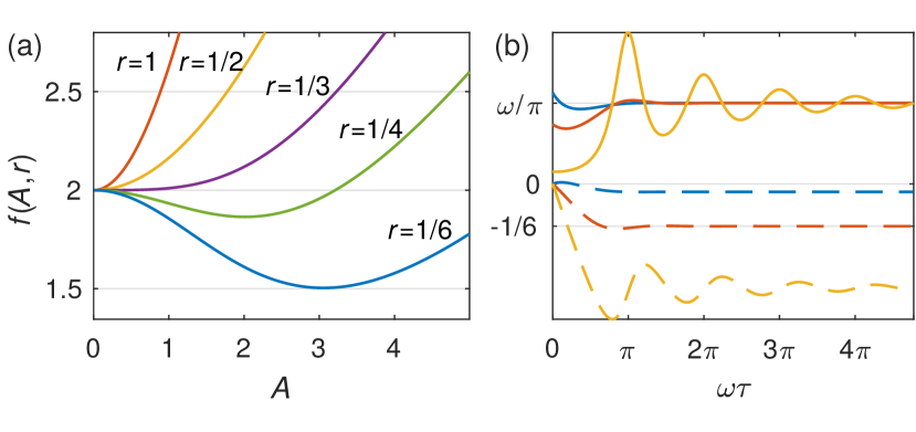
Figure 2: (a) Plot of the function $f(r,A)$ of Eq. (11), for selected values of the parameter $r$. The value $r=1/3$ is a critical one, below which a minimum below $1$ occurs at nonzero $A$. (b) Correlation function $\langle\dot{N}(0)\dot{N}(t)\rangle/\langle\dot{N}\rangle$ (solid) and its integral $\int_{0^{+}}^{t}d\tau[\langle\dot{N}(0)\dot{N}(\tau)\rangle/\langle\dot{N}\rangle-\langle\dot{N}\rangle]$ (dashed). The parameter $\gamma/(m\omega)$ has values $1.5$ (blue), $0.981$ (red), and $0.2$ (yellow).

The dispersion of ticks is calculated as Seifert (2010)

$$D_{N}=\frac{1}{2}\langle\dot{N}\rangle+\int_{0^{+}}^{\infty}d\tau\,[\langle\dot{N}(0)\dot{N}(\tau)\rangle-\langle\dot{N}\rangle^{2}].$$ (15)

The lower limit $0^{+}$ indicates that the trivial self-correlation of every tick at $\tau=0$ is excluded, it produces the first term. The correlation function $\langle\dot{N}(0)\dot{N}(\tau)\rangle/\langle\dot{N}\rangle$ [shown in Fig. 2(b)] can be interpreted as the probability density of a tick occurring at time $\tau$ given a tick at time $0$. We calculate it analytically from the Gaussian propagator  and evaluate the integral in Eq. (15) numerically. The mean and variance of the counter variable $y(t)$ can then be calculated using Eqs. (S.21 and 8), provided the timescale separation $k^{\pm}\gg\omega/\pi$ and $k^{\pm}\gg\gamma/m$ Note (1). For small damping $\gamma$, the correlation function exhibits oscillations with maxima at subsequent ticks, which are initially sharply peaked and then become broader. The time in between these peaks can have a sufficient negative contribution, so that the overall integral becomes less than $-\langle\dot{N}\rangle/6$, yielding $D_{N}/\langle\dot{N}\rangle<1/3$. This is the case for the damping below a certain critical value, determined numerically as $\gamma/(m\omega)\simeq 0.981$. Remarkably, this critical value presents still a fairly strong damping, with just one coherent oscillation discernible in Fig. 2b. For any damping weaker than that, the TUR is violated for matching affinity $A$.

In the limit of vanishing damping, $\gamma\to 0$, the sequence of ticks becomes deterministic (regardless of the energy, which is sampled initially from $p^{\mathrm{eq}}$). The counter system then behaves as a discrete-time Markov process, for which the possibility of violating the TUR (1) is well known Shiraishi (2017); Proesmans and Van den Broeck (2017). Yet, we show here that such a discrete-time process can be realised as a limiting case of a continuous one, without additional entropic cost. In accordance with the discrete-time TURs of Refs. Proesmans and Van den Broeck (2017) and Liu et al. (2020), our model allows for a vanishing uncertainty product (10) for $D_{N}/\langle\dot{N}\rangle\to 0$ and $A\to\infty$. The latter entails either divergent entropy production or vanishing speed $\langle\dot{y}\rangle$. For clocks that require the hand to move forward at a nonvanishing speed, a recent study shows that precision does indeed come at a minimal energetic cost Pearson et al. (2021).

Continuous model.

So far, we have shown that the TUR does not hold for systems consisting of a discrete and an underdamped continuous degree of freedom. We now show numerically that the TUR can also be broken with two continuous degrees of freedom. Moreover, we consider an escapement that, like in actual pendulum clocks, provides a feedback on the oscillator to sustain amplitudes beyond those of equilibrium oscillations.

We use an underdamped Langevin equation of the form

$$m\ddot{\boldsymbol{r}}=-\nabla V(\boldsymbol{r})-\gamma\dot{\boldsymbol{r}}+f^{\mathrm{ex}}\boldsymbol{e}_{y}+\boldsymbol{\xi}(t)$$ (16)

for the configuration $\boldsymbol{r}=(x,y)^{T}$, with the mass $m$, damping $\gamma$, a driving force $f^{\mathrm{ex}}$ acting in the $y$ direction, and a noise term $\boldsymbol{\xi}(t)$ with two independent components with the same properties as for the harmonic oscillator above. The potential is harmonic in $x$, with an additional coupling term, $V(\boldsymbol{r})=m\omega^{2}x^{2}/2+V_{\textup{c}}(\boldsymbol{r})$.

We choose the coupling term such that it reinforces the harmonic motion of an undamped oscillator of frequency $\omega$ and a certain amplitude $a$ in the $x$ direction while moving steadily at terminal velocity $f^{\mathrm{ex}}/\gamma$ in the $y$ direction. This ideal motion traces out the curve $\hat{x}(y)=a\sin(\omega y\gamma/f^{\mathrm{ex}})$, and we choose the coupling potential such that this curve is favoured, setting $V_{\textup{c}}(\boldsymbol{r})=\kappa[x-\hat{x}(y)]^{2}/2$, with some stiffness $\kappa$. Fig. 3(a) shows this potential and the ideal curve. For suitably chosen $\kappa$ and $a$, sample trajectories follow the ideal curve closely. The potential landscape acts as an escapement, providing potential barriers that impede the motion in the $y$ direction when it is too fast, and accelerates it when it is too slow.

We simulate the steady state of the system by numerically integrating the Langevin equation (16), using the method of Ref. Grønbech-Jensen and Farago (2013). The variance of $y(t)$ is calculated for samples of time windows of length $t$ taken from a long trajectory. The current $J_{y}=\left\langle y(t)\right\rangle/t$ (for any $t$) is evaluated as the average speed over the whole trajectory, and the entropy production rate follows as $\sigma=f^{\mathrm{ex}}J_{y}/T$.

Figure 3: (a) Potential landscape $V(x,y)$ serving as a continuous model for an escapement. The external force $f^{\mathrm{ex}}=1$ is indicated as a tilting in the $y$ direction. The ideal curve $\hat{x}(y)$ is shown as red dashed, with sample trajectories in white. Parameters: $\kappa=1$, $a=3$, $\omega=1$, $\gamma=0.1$, $T=1$, $m=1$. (b) Uncertainty product as a function of the length $t$ of the time window. The bound conjectured in Ref. Fischer et al. (2020) (solid line) corresponds to free diffusion in $y$ ($\kappa=0$, dark grey). This bound holds for the washboard potential $V_{c}(\boldsymbol{r})=(f^{\mathrm{ex}}\gamma/\omega)\sin(\omega y\gamma/f^{\mathrm{ex}})$ (light grey). For the escapement potential the bound is broken. In particular, the long-time limit is below the value $2$ relevant for the TUR (1) for all three combinations of the parameters $\kappa,a$ shown (red, blue, yellow). All other parameters as in (a).

As a result, the escapement mechanism suppresses fluctuations in the $y$ direction, compared to the fluctuations of an underdamped particle diffusing freely, see Fig. 3(b). In Ref. Fischer et al. (2020), it had been conjectured that free diffusion sets a lower bound on the uncertainty product [the left hand side of the TUR (1)] for underdamped dynamics on finite timescales. While this supposed bound holds true for most generic potential landscapes (and in particular for uncoupled dynamics, e.g., a washboard potential in the $y$ direction independent of $x$), it is broken for our design of an escapement. Violations occur for any $t>0$, and in particular in the long-time limit, over a robust range of the parameters $\kappa$ and $a$.

Outlook.

We have used a simple design of an escapement coupled to a pendulum to construct a counterexample to the TUR for underdamped dynamics. The considerations that have led to Eqs. (S.21)-(9) are specific for the model of the escapement, but completely general about the oscillator producing the ticks. The application to other physical systems may also be fruitful. For instance, for quantum systems exhibiting coherent oscillations, a general TUR of the form (1) could also be ruled out, in line with previous observations Brandner et al. (2018); Agarwalla and Segal (2018); Ptaszyński (2018). An atomic clock could hence yield precision beyond the limitations of the TUR as well.

Likewise, a thermodynamically consistent analysis of resistor-inductor-capacitor (RLC) circuits Freitas et al. (2020) could reveal coherent oscillations similar to those of the underdamped oscillator, showing that the TUR is broken not only for constant, external magnetic fields but also for fluctuating magnetic fields generated by the system itself. Steady state thermoelectric devices exploiting this fact could evade the trade-off between power, efficiency, and constancy that follows from the TUR Pietzonka and Seifert (2018), similar to cyclically driven heat engines Shiraishi et al. (2016); Holubec and Ryabov (2018).

Future research, systematically comparing different designs of escapement mechanisms and oscillator systems, may reveal ultimate thermodynamic bounds on the precision of autonomous clocks and complement thermodynamic uncertainty relations for underdamped dynamics.

Acknowledgments.

I thank Michael E. Cates for discussions and comments on the manuscript. I also thank Corpus Christi College, Cambridge for support through a nonstipendiary Junior Research Fellowship and inspiration about pendulum clocks. This work was funded by the European Research Council under the EU’s Horizon 2020 Program, Grant No. 740269.

Supplemental Material: Classical pendulum clocks break the thermodynamic uncertainty relation

.1 Correlations of the underdamped harmonic oscillator in equilibrium

First, we make the system dimensionless by scaling time as $\tilde{t}\equiv\omega t$, space as $\tilde{x}\equiv x\sqrt{m/T}/\omega$ and velocity as $\tilde{v}\equiv v\sqrt{m/T}/\omega^{2}$. The Langevin equation (12) of the main text then becomes

$$\partial_{\tilde{t}}\tilde{x} =\tilde{v},$$

$$\partial_{\tilde{t}}\tilde{v} =-\tilde{x}-\tilde{\gamma}\tilde{v}+\tilde{\xi}(\tilde{t}),$$ (S.1)

with a Gaussian white noise $\tilde{\xi}(\tilde{t})$ with correlations $\langle\tilde{\xi}(\tilde{t})\tilde{\xi}(\tilde{t}^{\prime})\rangle=2\tilde{\gamma}\delta(\tilde{t}-\tilde{t}^{\prime})$ and $\tilde{\gamma}\equiv\gamma/(m\omega)$. For the remainder of this Supplemental Material, we drop the tilde.

The equilibrium distribution in these reduced units is

$$p^{\mathrm{eq}}(x,v)=\frac{1}{2\pi}e^{-(x^{2}+v^{2})/2}.$$ (S.2)

We are interested in the fluctuations of the observable $\dot{N}=|v|\delta(x)$, with mean

$$\langle\dot{N}\rangle=\int dx\int dv\,p^{\mathrm{eq}}(x,v)\,\delta(x)|v|=1/\pi.$$ (S.3)

The propagator for the system, $p(x_{1},v_{1},t|x_{0},v_{0})$, gives the probability density to find the system in state $(x_{1},v_{1})$ at time $t$ provided that it had been in state $(x_{0},v_{0})$ at time $0$. With this propagator, the correlation function of the observable $\dot{N}$ can be written as

$$\langle\dot{N}(0)\dot{N}(t)\rangle =\int dx_{0}\int dv_{0}\int dx_{1}\int dv_{1}\,p^{\mathrm{eq}}(x_{0},v_{0})\,\delta(x_{0})|v_{0}|\,p(x_{1},v_{1},t|x_{0},v_{0})\,\delta(x_{1})|v_{1}|$$

$$=\int dv_{0}\int dv_{1}\,|v_{0}v_{1}|\,p^{\mathrm{eq}}(0,v_{0})\,p(0,v_{1},t|0,v_{0}).$$ (S.4)

As the solution of a 2-dimensional Ornstein-Uhlenbeck process, the propagator is Gaussian

$$p(\boldsymbol{z}_{1},t|\boldsymbol{z}_{0})=\frac{1}{2\pi\sqrt{\det\boldsymbol{\sigma}}}e^{-(\boldsymbol{z}_{1}-\boldsymbol{\mu})^{T}\boldsymbol{\sigma}^{-1}(\boldsymbol{z}_{1}-\boldsymbol{\mu})/2},$$ (S.5)

where we use a vectorial notation $\boldsymbol{z}\equiv(x,v)^{T}$. The mean $\boldsymbol{\mu}$ and the covariance $\boldsymbol{\sigma}$ satisfy the differential equations

$$\dot{\boldsymbol{\mu}} =-\boldsymbol{A}\boldsymbol{\mu}$$ (S.6)

$$\dot{\boldsymbol{\sigma}} =-\boldsymbol{A}\boldsymbol{\sigma}-\boldsymbol{\sigma}\boldsymbol{A}^{T}+\boldsymbol{D}$$ (S.7)

with the matrices

$$\boldsymbol{A}\equiv\left(\begin{matrix}0&-1\\ 1&\gamma\end{matrix}\right),\qquad\boldsymbol{D}\equiv\left(\begin{matrix}0&0\\ 0&2\gamma\end{matrix}\right)$$ (S.8)

and the initial conditions $\boldsymbol{\mu}(0)=\boldsymbol{z}_{0}$ and $\boldsymbol{\sigma}(0)=\boldsymbol{0}$ (the $2\times 2$ matrix containing zeros). For the evaluation of Eq. (S.4) we only need the initial condition of the form $\boldsymbol{z}_{0}=(0,v_{0})$, for which the solution of Eq. (S.6) yields $\boldsymbol{\mu}(t)=v_{0}\boldsymbol{\mu}_{0}(t)$ with

$$\boldsymbol{\mu}_{0}(t)=\frac{1}{\bar{\omega}}e^{-\gamma t/2}\left(\begin{matrix}\sin(\bar{\omega}t)\\ -(\gamma/2)\sin(\bar{\omega}t)+\bar{\omega}\cos(\bar{\omega}t)\end{matrix}\right)$$ (S.9)

and the frequency of the damped oscillator $\bar{\omega}\equiv\sqrt{1-\gamma^{2}/4}$. We consider only damping that is below critical, i.e., $\gamma<2$. Solving the set of linear differential equations for the coefficients of $\boldsymbol{\sigma}$ gives

$$\boldsymbol{\sigma}(t)=\left(\begin{matrix}1&0\\ 0&1\end{matrix}\right)+\frac{e^{-\gamma t}}{2\bar{\omega}}\left[\left(\begin{matrix}-2&\gamma\\ \gamma&-2\end{matrix}\right)+\left(\begin{matrix}\gamma/2&-1\\ -1&\gamma/2\end{matrix}\right)\gamma\cos(2\bar{\omega}t)+\left(\begin{matrix}-1&0\\ 0&1\end{matrix}\right)\gamma\bar{\omega}\sin(2\bar{\omega}t)\right].$$ (S.10)

Combining the Gaussian functions of the equilibrium distribution and the propagator, the correlation function (S.4) can be written as

$$\langle\dot{N}(0)\dot{N}(t)\rangle=\frac{1}{4\pi^{2}\sqrt{\det\boldsymbol{\sigma}}}\int dv_{0}\int dv_{1}\,|v_{0}v_{1}|\,\exp\left[-\frac{1}{2}\left(\begin{matrix}v_{0}\\ v_{1}\end{matrix}\right)\cdot\boldsymbol{\varSigma}\left(\begin{matrix}v_{0}\\ v_{1}\end{matrix}\right)\right].$$ (S.11)

Therein, the matrix $\boldsymbol{\varSigma}$ is given as

$$\boldsymbol{\varSigma}\equiv\left(\begin{matrix}1&0\\ 0&0\end{matrix}\right)+\boldsymbol{B}^{T}\boldsymbol{\sigma}^{-1}\boldsymbol{B}$$ (S.12)

with

$$\boldsymbol{B}\equiv\left(\begin{matrix}[\boldsymbol{\mu}_{0}(t)]_{1}&0\\ [\boldsymbol{\mu}_{0}(t)]_{2}&1\end{matrix}\right).$$ (S.13)

Finally, the Gaussian integral over $|v_{0}v_{1}|$ in Eq. (S.11) can be performed analytically, giving the result

$$\langle\dot{N}(0)\dot{N}(t)\rangle=\frac{1}{\pi^{2}\sqrt{\det\boldsymbol{\sigma}}\det\boldsymbol{\varSigma}}\left(1+\frac{|\varSigma_{12}|}{\sqrt{\det\boldsymbol{\varSigma}}}\arctan\frac{|\varSigma_{12}|}{\sqrt{\det\boldsymbol{\varSigma}}}\right).$$ (S.14)

The analytic expressions for the coefficients of the $2\times 2$ matrices can be recursively plugged into this result, however, the resulting expression is lengthy and cannot be simplified.

For a straightforward numerical integration of the correlation function, it is necessary that it does not show any divergence for $t\to 0^{+}$. Indeed, expanding all the terms for small $t$ to leading order as $\det\boldsymbol{\sigma}\approx t^{4}/3$, $\det\boldsymbol{\varSigma}\approx 3/t^{2}$, and $\varSigma_{12}\approx-1/t$, we get the finite limit

$$\lim_{t\to 0^{+}}\langle\dot{N}(0)\dot{N}(t)\rangle=\gamma\frac{6\sqrt{3}+\pi}{18\pi^{2}}.$$ (S.15)

.2 Timescale separation

In our general minimal model for an escapement, we assume that the distribution of the two possible states $y^{-}$ and $y^{+}$ of the counter variable relaxes instantaneously to the equilibrium distribution $p_{\pm}$ determined by the rates $k^{+}$ and $k^{-}$. This assumption is justified if these rates are large enough, such that the actual relaxation time of the counter $1/k\equiv 1/(k^{+}+k^{-})$ is much smaller than any relevant timescale of the oscillator process.

Yet, when we consider the underdamped harmonic oscillator, it may not be obvious to identify its relevant timescales. Here, two subsequent ticks (i.e., crossings of $x=0$) can be separated by a time interval smaller than any finite $1/k$. The following analysis shows that such events are sufficiently infrequent to not have a remaining contribution to the statistics of the counter variable $y$ in the limit $k\to\infty$.

Assume there is a tick happening at time $t=0$, where the oscillator crosses $x=0$ at speed $v_{0}$. Then, to generate the next tick, the oscillator needs to be transported back to the position $x=0$, crossing it at speed $v_{1}$ with sign opposite to $v_{0}$. As per the Langevin equation (S.1), there is both a ballistic and a diffusive contribution to this transport. For large $v_{0}$ and/or small $\gamma$, ballistic transport dominates, which causes the next tick at the time $t\simeq\pi$. Hence $1/k\ll\pi$ is one condition on the transition rates. Yet, for small $v_{0}$ and/or large $\gamma$, diffusive transport provides a shortcut to having a tick much earlier.

The rate of ticks at time $t>0$ conditioned on a tick at time $0$ at velocity $v_{0}$ is given by

$$\langle\dot{N}\rangle(t|v_{0})\equiv\int dv_{1}\,|v_{1}|\,p(0,v_{1},t|0,v_{0}),$$ (S.16)

with the Gaussian propagator introduced in the previous section. Results for various values of $v_{0}$ are shown in Fig. 4. To assess the behavior for small values of $t$, we expand every component of $\boldsymbol{\sigma}(t)$ and $\boldsymbol{\mu}(t)$ to leading order in $t$. Performing the Gaussian integral in Eq. (S.16) then yields the scale invariant form

$$\langle\dot{N}\rangle(t|v_{0})=\frac{\gamma}{v_{0}^{2}}\phi(t\gamma/v_{0}^{2})$$ (S.17)

with

$$\phi(u)\equiv\frac{\sqrt{3}}{2\pi u}e^{-1/u}+\frac{\sqrt{3}}{4\sqrt{\pi}u^{3/2}}e^{-3/(4u)}\operatorname{erf}\left(\frac{1}{2u}\right).$$ (S.18)

As shown in Fig. 4, this function has a distinct maximum at $u\sim 1$, which corresponds to the re-crossings of $x=0$ caused by the diffusive dynamics. For small $v_{0}^{2}/\gamma$, the corresponding maximum in $\langle\dot{N}\rangle(t|v_{0})$ can become indefinitely large. However, preceding this maximum we see an onset time where re-crossings are exponentially suppressed, for $t\gamma/v_{0}^{2}\ll 1$. This is the time it takes for the diffusive dynamics to reverse the sign of $v$ in order to enable a repeated crossing of $x=0$. This behavior is distinctive for underdamped dynamics, in contrast to overdamped dynamics where every crossing of a point is immediately followed by an infinite number of re-crossings.

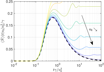
Figure 4: Rate of ticks in the time $t$ following a previous tick where the oscillator had the velocity $v_{0}$. Axes are scaled such that the scale invariant form (black dashed) that holds for $t\ll\pi$ becomes visible. Parameters: $\gamma=0.5$ and $v_{0}$ from $0.1$ (dark blue) to $0.8$ (yellow).

If the counter equilibrates within the time where re-crossings are suppressed, i.e., if $1/k\ll v_{0}^{2}/\gamma$, then the assumption that this equilibration happens instantaneously is justified. Next, we calculate the fraction of ticks in the stationary state where $|v_{0}|$ is below a certain small cutoff velocity $\hat{v}$,

$$\frac{\langle\dot{N}|{-\hat{v}<v_{0}<\hat{v}}\rangle}{\langle\dot{N}\rangle}=\frac{1}{\langle\dot{N}\rangle}\int dx\int_{-\hat{v}}^{\hat{v}}dv\,|v|\,\delta(x)\,p^{\mathrm{eq}}(x,v)=1-e^{-\hat{v}^{2}/2}\approx\hat{v}^{2}/2.$$ (S.19)

Thus, if $\gamma/k\ll 1$, or, more precisely, if we can find a $\hat{v}$ such that $\gamma/k\ll\hat{v}^{2}\ll 1$, then the assumption of the separation of timescales is justified for almost all ticks.

We now show explicitly that this separation of timescales leads indeed to the statistics of the counter variable $y(t)$ derived in the main text. For this purpose we consider the observables $N+(t)$ and $N^{-}(t)$, which count the number of increments and decrements of $y(t)$ up to time $t$. Using the variable $n(t)\in\{+,-\}$ that indicates whether the counter is in a state $y^{+}$ or $y^{-}$, these observables can be defined analogously to $N(t)$ through

$$N^{\pm}(t)=\int_{0}^{t}d\tau|v(\tau)|\,\delta[x(\tau)]\,\delta_{n(\tau^{-}),\pm},$$ (S.20)

where the Kronecker delta filters out ticks by the state of $n(t)$ ultimately prior to the tick. Thus, we have $N(t)=N^{+}(t)+N^{-}(t)$ and $y(t)=N^{+}(t)-N^{-}(t)$. The average of $y(t)$ can be written as

$$\left\langle y(t)\right\rangle=t\int dv\,p^{\mathrm{eq}}(v)\,\left[\langle\dot{N}^{+}|v\rangle-\langle\dot{N}^{-}|v\rangle\right],$$ (S.21)

with steady state averages conditioned on the velocity $v$. Time reversal symmetry in equilibrium requires that Eq. (S.17) also gives the rate of ticks at the time $t$ before another tick, i.e., $\langle\dot{N}\rangle(t|v_{0})=\langle\dot{N}\rangle(-t|v_{0})$. Hence, we know that for $|v|>\hat{v}\gg\sqrt{\gamma/k}$ the variable $n(t)$ will have had time to equilibrate since the last tick, such that $\langle\dot{N}^{\pm}|v\rangle=p^{\pm}\langle\dot{N}|v\rangle$. We can therefore rewrite Eq. (S.21) as

$$\left\langle y(t)\right\rangle=t(p^{+}-p^{-})\langle\dot{N}\rangle+t\int_{-\hat{v}}^{\hat{v}}dv\,p^{\mathrm{eq}}(v)\,\left[\langle\dot{N}^{+}|v\rangle-\langle\dot{N}^{-}|v\rangle-(p^{+}-p^{-})\langle\dot{N}|v\rangle\right].$$ (S.22)

For $v\sim\sqrt{\gamma/k}$, the calculation of $\langle\dot{N}^{\pm}|v\rangle$ is far less trivial (and probably not possible within the Gaussian formalism). Yet, as we consider small $\hat{v}$, it only matters that the integrand does not diverge. Indeed, since $0\leq\langle\dot{N}^{\pm}|v\rangle\leq\langle\dot{N}|v\rangle=\sqrt{2\pi}|v|$, we find that the integral in Eq. (S.22) vanishes like $\hat{v}^{2}$. The remaining first term is equal to the result obtained in the main text based on the assumption of instantaneous equilibration.

For the evaluation of the dispersion of $y(t)$, we consider the integral

$$D_{y}= \lim_{t\to\infty}\frac{1}{2t}\mathrm{Var}\,y(t)$$

$$\approx\frac{1}{2}\langle\dot{N}\rangle+\int_{0^{+}}^{\hat{t}}d\tau\left[\langle\dot{N}^{+}(0)\dot{N}^{+}(\tau)\rangle-\langle\dot{N}^{+}(0)\dot{N}^{-}(\tau)\rangle-\langle\dot{N}^{-}(0)\dot{N}^{+}(\tau)\rangle+\langle\dot{N}^{-}(0)\dot{N}^{-}(\tau)\rangle-(\langle\dot{N}^{+}\rangle-\langle\dot{N}^{-}\rangle)^{2}\right],$$ (S.23)

where the upper limit $\hat{t}$ is chosen much larger than both the timescale $t\sim\pi$ for oscillations and the timescale $t\sim 1/\gamma$ for diffusion. On this timescale, the dynamics of the system decorrelates, such that the autocorrelation function of $\dot{y}(t)$ [the integrand of Eq. (S.23)] tends exponentially to zero. The choice of a large but finite $\hat{t}$ will be convenient in the following analysis. The error incurred by this approximation is exponentially small and therefore negligible.

If the equilibration of the counter after a tick was instantaneous, we would have

$$\langle\dot{N}^{+}(0)\dot{N}^{+}(\tau)\rangle=p^{+}p^{+}\langle\dot{N}(0)\dot{N}(\tau)\rangle, \langle\dot{N}^{+}(0)\dot{N}^{-}(\tau)\rangle=p^{+}p^{-}\langle\dot{N}(0)\dot{N}(\tau)\rangle,$$

$$\langle\dot{N}^{-}(0)\dot{N}^{+}(\tau)\rangle=p^{-}p^{+}\langle\dot{N}(0)\dot{N}(\tau)\rangle, \langle\dot{N}^{-}(0)\dot{N}^{-}(\tau)\rangle=p^{-}p^{-}\langle\dot{N}(0)\dot{N}(\tau)\rangle.$$ (S.24)

Plugging this into Eq. (S.23), along with $\langle\dot{N}^{\pm}\rangle=p^{\pm}\langle\dot{N}\rangle$ then leads to the diffusion coefficient derived in the main text.

For large but finite $k$, deviations from Eq. (S.24) will surely occur for times $\tau$ comparable to $1/k$. We therefore split the integral in Eq. (S.23) into $0<\tau<\hat{v}^{2}/\gamma$ and $\hat{v}^{2}/\gamma\leq\tau<\hat{t}$. For the first part, we see in the following way that the integrand cannot have any singularities: Since $\dot{N}^{\pm}\geq 0$, all the four terms $\langle\dot{N}^{\pm}(0)\dot{N}^{\pm}(\tau)\rangle$ are bounded from below by zero. Moreover, they add up to

$$\langle\dot{N}^{+}(0)\dot{N}^{+}(\tau)\rangle+\langle\dot{N}^{+}(0)\dot{N}^{-}(\tau)\rangle+\langle\dot{N}^{-}(0)\dot{N}^{+}(\tau)\rangle+\langle\dot{N}^{-}(0)\dot{N}^{-}(\tau)\rangle=\langle\dot{N}(0)\dot{N}(\tau)\rangle.$$ (S.25)

Hence, each of the four terms is bounded from above by $\langle\dot{N}(0)\dot{N}(\tau)\rangle$, which we have already shown to be finite for small $\tau$ in Eq. (S.15). The part of the integral in Eq. (S.23) with $0<\tau<\hat{v}^{2}/\gamma$ therefore vanishes as $\hat{v}\to 0$.

For times $\tau\geq\hat{v}^{2}/\gamma$, deviations from Eq. (S.24) are still possible. Even though there is enough time for $n(t)$ to equilibrate between two ticks at times $0$ and $\tau$, further ticks may have occurred briefly before these two points in time, bringing $n(t)$ out of equilibrium. For a more detailed analysis, consider

$$\int_{\hat{v}^{2}/\gamma}^{\hat{t}}d\tau\,\langle\dot{N}^{+}(0)\dot{N}^{+}(\tau)\rangle=\int_{\hat{v}^{2}/\gamma}^{\hat{t}}d\tau\int dv_{0}\int dv_{1}\,p(v_{0},v_{1},\tau)\,\langle\dot{N}^{+}(0)\dot{N}^{+}(\tau)|v_{0},v_{1}\rangle$$ (S.26)

[and analogously for the other three similar terms in Eq. (S.23)]. Here we have conditioned on the velocities $v_{0}$ and $v_{1}$ at times $0$ and $\tau$ and averaged using their joint distribution $p(v_{0},v_{1},\tau)$. When both $v_{0}$ and $v_{1}$ are greater than $\hat{v}$, enough time will have passed since the respective previous ticks to equilibrate the variable $n(t)$, such that we obtain $\langle\dot{N}^{+}(0)\dot{N}^{+}(\tau)|v_{0},v_{1}\rangle=p^{+}p^{+}\langle\dot{N}(0)\dot{N}(\tau)|v_{0},v_{1}\rangle$. Writing

$$\int_{\hat{v}^{2}/\gamma}^{\hat{t}}d\tau\,\langle\dot{N}^{+}(0)\dot{N}^{+}(\tau)\rangle= p^{+}p^{+}\int_{\hat{v}^{2}/\gamma}^{\hat{t}}d\tau\,\langle\dot{N}(0)\dot{N}(\tau)\rangle$$

$$+\int_{\hat{v}^{2}/\gamma}^{\hat{t}}d\tau\int^{\prime}dv_{0}\int^{\prime}dv_{1}\,p(v_{0},v_{1},\tau)\,[\langle\dot{N}^{+}(0)\dot{N}^{+}(\tau)|v_{0},v_{1}\rangle-p^{+}p^{+}\langle\dot{N}(0)\dot{N}(\tau)|v_{0},v_{1}\rangle],$$ (S.27)

where the integrals marked by ^′ run over the space where $v_{0}$ or $v_{1}$ are smaller than $\hat{v}$, it now remains to be shown that the second line vanishes as $\hat{v}\to 0$. Following the same logic as above, the terms $\langle\dot{N}^{\pm}(0)\dot{N}^{\pm}(\tau)|v_{0},v_{1}\rangle$ are bounded from below by $0$ and from above by $\langle\dot{N}(0)\dot{N}(\tau)|v_{0},v_{1}\rangle$. Thus, it is sufficient to show that the integral over the latter vanishes. Its part where $|v_{0}|<\hat{v}$ reads

$$\int_{\hat{v}^{2}/\gamma}^{\hat{t}}d\tau\int_{-\hat{v}}^{\hat{v}}dv_{0}\int_{-\infty}^{\infty}dv_{1}\,p(v_{0},v_{1},\tau)\,\langle\dot{N}(0)\dot{N}(\tau)|v_{0},v_{1}\rangle=\int_{\hat{v}^{2}/\gamma}^{\hat{t}}d\tau\int_{-\hat{v}}^{\hat{v}}dv_{0}\,|v_{0}|\,p^{\mathrm{eq}}(0,v_{0})\,\langle\dot{N}\rangle(\tau|v_{0}),$$ (S.28)

where we identify the function from Eq. (S.16). The periodically recurring ticks incurred by ballistic transport happen on average at a finite rate $1/\pi$, their contribution to above integral must therefore vanish for small $\hat{v}$. We therefore focus on the immediate re-crossings incurred by diffusive transport, captured by the function $\phi(u)$ in Eq. (S.17),

$$\int_{\hat{v}^{2}/\gamma}^{\hat{t}}d\tau\int_{-\hat{v}}^{\hat{v}}dv_{0}\,|v_{0}|\,p^{\mathrm{eq}}(0,v_{0})\,\frac{\gamma}{v_{0}^{2}}\phi(t\gamma/v_{0}^{2})=\int_{-\hat{v}}^{\hat{v}}dv_{0}\,|v_{0}|\,p^{\mathrm{eq}}(0,v_{0})\,\int_{\hat{v}^{2}/v_{0}^{2}}^{\hat{t}\gamma/v_{0}^{2}}du\,\phi(u)\sim\hat{v}^{2}\ln\frac{\hat{t}\gamma}{\hat{v}^{2}}.$$ (S.29)

For the estimation of the value of the last integral we have used the fact that we only need $\phi(u)$ for $u>1$, which is at first finite (see Fig. 4) and then, for larger $u$, gets dominated by the first term in Eq. (S.18) scaling like $u^{-1}$. As a result, we see that the integral vanishes as $\hat{v}$ gets small.

For the remaining part of the integral in the second line of Eq. (S.27) we calculate

$$\int_{\hat{v}^{2}/\gamma}^{\hat{t}}d\tau\int_{|v_{0}|>\hat{v}}dv_{0}\int_{-\hat{v}}^{\hat{v}}dv_{1}\,p(v_{0},v_{1},\tau)\,\langle\dot{N}(0)\dot{N}(\tau)|v_{0},v_{1}\rangle$$

$$\qquad<\int_{\hat{v}^{2}/\gamma}^{\hat{t}}d\tau\int_{-\infty}^{\infty}dv_{0}\int_{-\hat{v}}^{\hat{v}}dv_{1}\,p(v_{0},v_{1},\tau)\,\langle\dot{N}(0)\dot{N}(\tau)|v_{0},v_{1}\rangle$$

$$\qquad\qquad=\int_{\hat{v}^{2}/\gamma}^{\hat{t}}d\tau\int_{-\hat{v}}^{\hat{v}}dv_{1}\,|v_{1}|\,p^{\mathrm{eq}}(0,v_{1})\,\langle\dot{N}\rangle(\tau|v_{1})\sim\hat{v}^{2}\ln\frac{\hat{t}\gamma}{\hat{v}^{2}}.$$ (S.30)

In the second line, we have used the positivity of the integrand to extend the integration space, and in the third line the symmetry of the correlation function with respect to $\tau$ to arrive at the same integral as in Eq. (S.29). As a result, we see that the second line in Eq. (S.27) vanishes altogether for small $\hat{v}$, such that the simple expression for the dispersion of $y(t)$ from the main text is recovered.

References

- Marrison (1948) W. A. Marrison, “The evolution of the quartz crystal clock,” Bell Syst. Tech. J. 27, 510 (1948).
- Horowitz and Gingrich (2020) J. M. Horowitz and T. R. Gingrich, “Thermodynamic uncertainty relations constrain non-equilibrium fluctuations,” Nat. Phys. 16, 15 (2020).
- Barato and Seifert (2015) A. C. Barato and U. Seifert, “Thermodynamic uncertainty relation for biomolecular processes,” Phys. Rev. Lett. 114, 158101 (2015).
- Gingrich et al. (2016) T. R. Gingrich, J. M. Horowitz, N. Perunov, and J. L. England, “Dissipation bounds all steady-state current fluctuations,” Phys. Rev. Lett. 116, 120601 (2016).
- Pietzonka et al. (2017) P. Pietzonka, F. Ritort, and U. Seifert, “Finite-time generalization of the thermodynamic uncertainty relation,” Phys. Rev. E 96, 012101 (2017).
- Horowitz and Gingrich (2017) J. M. Horowitz and T. R. Gingrich, “Proof of the finite-time thermodynamic uncertainty relation for steady-state currents,” Phys. Rev. E 96, 020103(R) (2017).
- Seifert (2018) U. Seifert, “From stochastic thermodynamics to thermodynamic inference,” Annu. Rev. Condens. Matter Phys. 10, 171 (2019).
- Dechant and Sasa (2018a) A. Dechant and S.-i. Sasa, “Entropic bounds on currents in Langevin systems,” Phys. Rev. E 97, 062101 (2018a).
- Dechant and Sasa (2018b) A. Dechant and S.-i. Sasa, “Current fluctuations and transport efficiency for general Langevin systems,” J. Stat. Mech. 063209 (2018b).
- Fischer et al. (2018) L. P. Fischer, P. Pietzonka, and U. Seifert, “Large deviation function for a driven underdamped particle in a periodic potential,” Phys. Rev. E 97, 022143 (2018).
- Van Vu and Hasegawa (2019) T. Van Vu and Y. Hasegawa, “Uncertainty relations for underdamped Langevin dynamics,” Phys. Rev. E 100, 032130 (2019).
- Lee et al. (2019) J. S. Lee, J.-M. Park, and H. Park, “Thermodynamic uncertainty relation for underdamped Langevin systems driven by a velocity-dependent force,” Phys. Rev. E 100, 062132 (2019).
- Vo et al. (2020) V. T. Vo, T. Van Vu, and Y. Hasegawa, “Unified approach to classical speed limit and thermodynamic uncertainty relation,” Phys. Rev. E 102, 062132 (2020).
- Lee et al. (2021) J. S. Lee, J.-M. Park, and H. Park, “Universal form of thermodynamic uncertainty relation for Langevin dynamics,” Phys. Rev. E 104, L052102 (2021).
- Brandner et al. (2018) K. Brandner, T. Hanazato, and K. Saito, “Thermodynamic bounds on precision in ballistic multiterminal transport,” Phys. Rev. Lett. 120, 090601 (2018).
- Chun et al. (2019) H.-M. Chun, L. P. Fischer, and U. Seifert, “Effect of a magnetic field on the thermodynamic uncertainty relation,” Phys. Rev. E 99, 042128 (2019).
- Fischer et al. (2020) L. P. Fischer, H.-M. Chun, and U. Seifert, “Free diffusion bounds the precision of currents in underdamped dynamics,” Phys. Rev. E 102, 012120 (2020).
- Barato and Seifert (2016) A. C. Barato and U. Seifert, “Cost and precision of Brownian clocks,” Phys. Rev. X 6, 041053 (2016).
- Proesmans and Van den Broeck (2017) K. Proesmans and C. Van den Broeck, “Discrete-time thermodynamic uncertainty relation,” EPL (Europhysics Letters) 119, 20001 (2017).
- Koyuk et al. (2019) T. Koyuk, U. Seifert, and P. Pietzonka, “A generalization of the thermodynamic uncertainty relation to periodically driven systems,” J. Phys. A: Math. Theor. 52, 02LT02 (2019).
- Barato et al. (2018) A. C. Barato, R. Chetrite, A. Faggionato, and D. Gabrielli, “Bounds on current fluctuations in periodically driven systems,” New J. Phys. 20, 103023 (2018).
- Koyuk and Seifert (2020) T. Koyuk and U. Seifert, “Thermodynamic uncertainty relation for time-dependent driving,” Phys. Rev. Lett. 125, 260604 (2020).
- Barato and Seifert (2017) A. C. Barato and U. Seifert, “Thermodynamic cost of external control,” New J. Phys. 19, 073021 (2017).
- Seifert (2010) U. Seifert, “Generalized Einstein or Green-Kubo relations for active biomolecular transport,” Phys. Rev. Lett. 104, 138101 (2010).
- Note (1) See Supplemental Material appended below.
- Shiraishi (2017) N. Shiraishi, “Finite-time thermodynamic uncertainty relation do not hold for discrete-time Markov process,” (2017), arXiv:1706.00892 .
- Liu et al. (2020) K. Liu, Z. Gong, and M. Ueda, “Thermodynamic uncertainty relation for arbitrary initial states,” Phys. Rev. Lett. 125, 140602 (2020).
- Pearson et al. (2021) A. N. Pearson, Y. Guryanova, P. Erker, E. A. Laird, G. A. D. Briggs, M. Huber, and N. Ares, “Measuring the thermodynamic cost of timekeeping,” Phys. Rev. X 11, 021029 (2021).
- Grønbech-Jensen and Farago (2013) N. Grønbech-Jensen and O. Farago, “A simple and effective Verlet-type algorithm for simulating Langevin dynamics,” Mol. Phys. 111, 983 (2013).
- Agarwalla and Segal (2018) B. K. Agarwalla and D. Segal, “Assessing the validity of the thermodynamic uncertainty relation in quantum systems,” Phys. Rev. B 98, 155438 (2018).
- Ptaszyński (2018) K. Ptaszyński, “Coherence-enhanced constancy of a quantum thermoelectric generator,” Phys. Rev. B 98, 085425 (2018).
- Freitas et al. (2020) N. Freitas, J.-C. Delvenne, and M. Esposito, “Stochastic and quantum thermodynamics of driven RLC networks,” Phys. Rev. X 10, 031005 (2020).
- Pietzonka and Seifert (2018) P. Pietzonka and U. Seifert, “Universal trade-off between power, efficiency, and constancy in steady-state heat engines,” Phys. Rev. Lett. 120, 190602 (2018).
- Shiraishi et al. (2016) N. Shiraishi, K. Saito, and H. Tasaki, “Universal trade-off relation between power and efficiency for heat engines,” Phys. Rev. Lett. 117, 190601 (2016).
- Holubec and Ryabov (2018) V. Holubec and A. Ryabov, “Cycling tames power fluctuations near optimum efficiency,” Phys. Rev. Lett. 121, 120601 (2018).