Direct numerical simulation of low Reynolds number oscillating boundary layers on adiabatic slopes

Abstract

We investigate the instabilities and transition mechanisms of Boussinesq stratified boundary layers on sloping boundaries when subjected to oscillatory body forcing parallel to the slope. Such conditions are typical of the boundary layers generated by low wavenumber internal tides sloshing up and down adiabatic abyssal slopes in the absence of mean flows, high wavenumber internal tides, and resonant tide-bathymetry interactions. We examine flows within a region of non-dimensional parameter space typical of the mid- to low-latitude oceanic $M_{2}$ tides on hydraulically smooth abyssal slopes by direct numerical simulation. We find that at low Reynolds numbers transition-to-turbulence pathways arise from both shear and gravitational instabilities, and we find that the boundary layers are stabilized by increased outer boundary layer stratification during the downslope oscillation phase. However, if rotation is significant (low slope Burger numbers) we find that boundary layer turbulence is sustained throughout the oscillation period, resembling Stokes-Ekman layer turbulence. Our results suggest that oscillating boundary layers on smooth abyssal slopes created by low wavenumber $M_{2}$ tides do not cause significant irreversible turbulent buoyancy flux (mixing) and that flat-bottom dissipation rate models derived from the tide amplitude are accurate within an order of magnitude.

1 Introduction

Irreversible buoyancy flux convergence within oscillating stratified boundary layers on sloping bathymetry in the abyss may be a significant mechanism driving the deep branch of the global overturning circulation (Ferrari et al. (2016)). The boundary layers, combined with other bottom-intensified sources of turbulence, such as the breaking of internal waves, contribute to observed patterns of intense irreversible buoyancy flux convergence (Polzin (1996)). How unstable are these boundary layers on typical abyssal slopes, and what are the instability mechanisms? In this article, we employ theory and direct numerical simulations to investigate the pathways between laminar, transitional, and turbulent states of boundary layers that are forced by the $M_{2}$ barotropic tide and occur on hydraulically smooth abyssal slopes in the absence of forcing by high-wavenumber internal waves, mean flows, far-field turbulence on larger scales, and resonant tidal-bathymetric interaction.

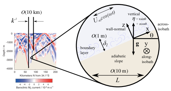
Figure 1: Illustration of NRBTBL length scales and geometry.

The M₂ tide velocity contour plot on the left is from Zilberman et al. (2009).

The boundary layers are formed as momentum and buoyancy are diffused by no-slip and adiabatic boundary conditions on sloping bathymetry as low-wavenumber internal waves heave isopycnals (constant-density contours) up and down slopes. Figure 1 illustrates the scale separations between the horizontal length scale of baroclinic tide generation, $k^{-1}$, (Garrett & Kunze (2007)), the excursion length scale of the tide, $L$, and the largest boundary layer length scale, $\delta_{l}$. The excursion length scale, $L$, is the characteristic scale of the across-isobath distance between the trajectory extrema in the inviscid problem, defined

$$L\sim{}\frac{U_{\infty}}{\omega},$$ (1)

where $U_{\infty}$ is the barotropic tide amplitude projected onto the across-slope tangential coordinate ($x$) and $\omega$ is the tide frequency. We assume that the slope curvature can be well approximated as constant on scales of the order of the excursion length, $L$. Thus the boundary layers investigated in this Article apply to boundary layer flows on hydraulically smooth slopes where the excursion parameter

$$\mathcal{E}=kL,$$ (2)

is small, $\mathcal{E}\ll 1$. The excursion parameter $\mathcal{E}$ is the ratio of net fluid advection by the barotropic tide to the topographic length. The baroclinic response to the barotropic forcing is highly nonlinear for large excursion parameter flows $\mathcal{E}$ (Bell (1975a), Bell (1975b), Garrett & Kunze (2007), Sarkar & Scotti (2017)). Here, we investigate the dynamics on scales at or smaller than the excursion length, thus we assume that the baroclinic tide (a.k.a. internal waves) generated by bathymetric features with horizontal length scales of $k^{-1}$ can be locally approximated as irrotational over $L$. Therefore we assume that the baroclinic tide can be modeled as an across-isobath oscillating body force on the scale of the excursion length.

Our objectives are 1) to determine if these boundary layers are laminar, transitional, intermittent, or fully turbulent for typical abyssal ocean non-dimensional parameters associated with the $M_{2}$ tide, 2) to investigate the transition mechanisms, and 3) to test back-of-the-envelope estimation for barotropic tide dissipation rates at the seafloor. This Article is organized as follows. In Problem formulation we discuss the relevant governing equations and non-dimensional parameters. In Linear Flow Solutions we investigate analytical solutions for the laminar flows to estimate the necessary conditions for boundary layer gravitational instabilities. In Nonlinear Flow Solutions we analyze the stability of simulated boundary layers, and in Conclusions we summarize the observed transition mechanisms and drag coefficients.

2 Problem formulation

The flows examined in this study subject to a body force in the across-isobath, or streamwise, direction (the $x$ direction in Figure 1),

$$F_{d}(t_{\mathrm{d}})=-\Real[A_{\mathrm{d}}\text{ie}^{\text{i}\omega t_{\mathrm{d}}}],$$ (3)

where $A_{\mathrm{d}}$ is the dimensional amplitude of the pressure gradient $\partial_{x}\tilde{P}_{\mathrm{d}}$ and $t_{\mathrm{d}}$ is dimensional time.

Several geometric and physical approximations are invoked for the sake of tractibility and conceptual simplicity. The flow is approximated as Boussinesq: the density variations are small enough that the incompressibility condition is justified, and Joule heating (increases of internal energy due to the viscous dissipation of mechanical energy) is neglected. We idealize abyssal buoyancy as a linear function of temperature alone.

A Cartesian coordinate system, rotated $\theta$ radians counterclockwise above the horizontal (Figure 1), was chosen for analytical convenience. The $z$ coordinate is the wall-normal (or transverse) coordinate, which is at angle $\theta$ from the vertical coordinate (the coordinate anti-parallel to the gravity). To distinguish between the slope-normal and vertical coordinates, the vertical coordinate (and vertical velocities, fluxes, etc) in the direction normal to Earth’s surface will be denoted as $\eta$, such that $\eta=x\sin\theta+z\cos\theta$, shown in Figure 1.

The non-dimensional Boussinesq governing equations for conservation of mass, momentum, and thermodynamic energy for the flow are

$$\partial_{x}\tilde{u} +\partial_{y}\tilde{v}+\partial_{z}\tilde{w}=0,$$ (4)

$$\mathrm{d}_{t}\tilde{{u}} =\frac{1}{\textit{Ro}}\tilde{v}-\partial_{x}\tilde{p}+\frac{1}{\Rey_{L}}\big{(}\partial_{xx}+\partial_{yy}+\partial_{zz}\big{)}\tilde{u}+\textit{C}^{2}\tilde{b}+F(t)$$ (5)

$$\mathrm{d}_{t}\tilde{{v}} =-\frac{1}{\textit{Ro}}\tilde{u}-\partial_{y}\tilde{p}+\frac{1}{\Rey_{L}}\big{(}\partial_{xx}+\partial_{yy}+\partial_{zz}\big{)}\tilde{v},$$ (6)

$$\mathrm{d}_{t}\tilde{{w}} =-\partial_{z}\tilde{p}+\frac{1}{\Rey_{L}}\big{(}\partial_{xx}+\partial_{yy}+\partial_{zz}\big{)}\tilde{w}+\textit{C}^{2}\tilde{b}\cot\theta,$$ (7)

$$\mathrm{d}_{t}\tilde{{b}} =\frac{1}{\Pran\hskip 0.85358pt\Rey_{L}}\big{(}\partial_{xx}+\partial_{yy}+\partial_{zz}\big{)}\tilde{b},$$ (8)

where $\mathrm{d}_{t}=\partial_{t}+\tilde{\mathbf{u}}\cdot\nabla$ and $F(t)=F_{\mathrm{d}}(t_{\mathrm{d}})/(U_{\infty}\omega)=A\sin(t)$. The variables are non-dimensionalized as follows (subscript “d” denoting dimensional variables):

$$\mathbf{x}={\mathbf{x}_{\text{d}}}/{L},\qquad\tilde{\mathbf{u}}={\tilde{\mathbf{u}}_{\text{d}}}/{U_{\scalebox{0.9}{$\scriptscriptstyle\infty$}}},\qquad t={\omega}{t_{\text{d}}},\qquad\tilde{p}={\tilde{p}_{\text{d}}}/{U_{\scalebox{0.9}{$\scriptscriptstyle\infty$}}^{2}},\qquad\tilde{b}={\tilde{b}_{\text{d}}}/{(LN^{2}\sin\theta)},$$ (9)

where the reference density $\rho_{0}$ is absorbed into the mechanical pressure $p_{\text{d}}$ such that it has units J kg^-1. $N^{2}$ is the square of the buoyancy frequency (the natural frequency associated with the restoring force of stratification). The buoyancy is defined as the acceleration associated with density anomalies, $b_{\mathrm{d}}=g(\rho_{0}-\rho)/\rho_{0}$, where $g$ is the (constant) gravity and $\rho$ is the density.

Despite the assumptions and idealizations listed above, the dynamical parameter space is vast. The relevant non-dimensional ratios are the Prandtl number $\Pran$, the slope Rossby number Ro, the slope frequency ratio C, and Stokes layer Reynolds number $\Rey$. In this study, the Stokes layer Reynolds number is referred to in the analysis of the flow instead of the excursion length Reynolds number

$$\Rey_{L}=\frac{U_{\infty}{}L}{\nu}=\frac{U_{\infty}^{2}}{\nu\omega},$$ (10)

because the Stokes layer Reynolds number is common in literature regarding oscillating boundary layers. The Prandtl and Stokes layer Reynolds numbers are defined as:

$$\Pran =\frac{\nu}{\kappa},$$ (11)

$$\Rey =\frac{U_{\infty}\delta}{\nu}=\sqrt{2\Rey_{L}},$$ (12)

where $\kappa$ is the molecular diffusivity of buoyancy and $\nu$ is the kinematic viscosity of abyssal seawater, and where the Stokes’ layer thickness is:

$$\delta=\sqrt{2\nu/\omega}.$$ (13)

The slope frequency ratio is defined as the ratio of the projection of the buoyant acceleration onto the across slope ($x$) direction (parallel to the forcing) to the acceleration of the oscillatory forcing,

$$\textit{C}=\frac{N\sin\theta}{\omega}.$$ (14)

The slope frequency ratio was first identified as an important ratio for describing the boundary layer by Hart (1971) (who denoted it as $\mathrm{Q}$, where $\mathrm{Q}=\textit{C}^{2}$), while the frequency ratio $N/\omega$ emerges as an important measure of the role of stratification in the stratified form of Stokes’ second problem (Gayen & Sarkar (2010a)). The slope frequency ratio is indicative of the degree of resonance between the oscillation body forcing and the buoyant restoring force.

Finally, the fourth non-dimensional ratio is slope Rossby number,

$$\mathrm{Ro}=\frac{\omega}{f\cos\theta},$$ (15)

which indicates the ratio of the influence of planetary vorticity (projected onto the wall normal direction) relative to vorticity with a characteristic time scale of the tide period, $\omega^{-1}$. For the finite Rossby number cases examined, $\omega$ is the M₂ tide frequency, the Coriolis parameter, $f$, is $10^{-4}$ s^-1, and the range of slope angles investigated are within $0<\theta\leq 14^{\circ}$. Therefore, the slope Rossby number is approximately 1.4 for all of the rotating reference frame flows investigated.

2.1 Invisicid, linear flow

The inviscid, linearized form of the governing equations (Equations 4-8) describe the heaving of isopycnals up and down the slope,

$$\partial_{t}\tilde{{u}} =\frac{1}{\textit{Ro}}\tilde{v}+\textit{C}^{2}\tilde{b}+F(t),$$ (16)

$$\partial_{t}\tilde{{v}} =-\frac{1}{\textit{Ro}}\tilde{u},$$ (17)

$$\partial_{t}\tilde{{b}} =-\tilde{{u}}.$$ (18)

Crucially, the solutions to Equations 16-18 prescribe the amplitude of the non-dimensional body force

$$A =\Big{(}\textit{C}^{2}+\frac{1}{\textit{Ro}^{2}}-1\Big{)},$$ (19)

where $A_{\mathrm{d}}=AU_{\infty}\omega$. The solutions to Equations 18-18 are

$$\tilde{{u}}(t) =-\cos(t),$$ (20)

$$\tilde{{v}}(t) =\textit{Ro}^{-1}\sin(t),$$ (21)

$$\tilde{{b}}(t) =\sin(t).$$ (22)

2.2 Resonance

The amplitude of the oscillating pressure gradient forcing $F(t)$ in equation 16 (the last term on the right hand side), vanishes if the critical slope condition

$$\textit{C}^{2}+\frac{1}{\textit{Ro}^{2}}-1=0,$$ (23)

is satisfied. Furthermore, if Equation 23 is satisfied, the energy of the inviscid baroclinic tide is tightly focused into narrow beams that follow the curvature of the bathymetry (Balmforth et al. (2002)); therefore, the assumption of locally irrotational flow breaks down at critical slope, even on length scales much less than $L$. At critical slope Equation 3 is no longer a valid approximation of the low-wavenumber baroclinic response to the barotropic tidal forcing.

Equation 23 is formally consistent with internal wave theory. In internal wave theory, critical slopes are defined by:

$$\tan\theta_{c}=\sqrt{\frac{\omega^{2}-f^{2}}{N^{2}-\omega^{2}}},$$ (24)

where $\theta_{c}$ is the critical slope angle. If the slope angle $\theta\neq\theta_{c}$, then Equation 19 is satisfied, $A\neq 0$. Equation 19 can be rearranged to obtain

$$\tan\theta=\sqrt{\frac{\omega^{2}(1+A)-f^{2}}{N^{2}-\omega^{2}(1+A)}}.$$ (25)

Therefore the criticality condition in Equation 23 is just a rearrangement of the criticality condition defined by the slope parameter $\epsilon$ from internal wave theory:

$$\epsilon=\frac{\tan\theta}{\tan\theta_{c}},$$ (26)

where criticality states are defined:

if $$\quad A<0\quad\text{then}\quad\epsilon<1\qquad\rightarrow\qquad\theta\hskip 4.83694pt\text{is subcritical},$$

if $$\quad A=0\quad\text{then}\quad\epsilon=1\qquad\rightarrow\qquad\theta\hskip 4.83694pt\text{is critical},$$

if $$\quad A>0\quad\text{then}\quad\epsilon>1\qquad\rightarrow\qquad\theta\hskip 4.83694pt\text{is supercritical}.$$

2.3 Boundary conditions

At the solid boundary at $z=0$, the boundary conditions on the total velocity are no-slip and impermeability

$$\tilde{\mathbf{u}}=0,$$ (27)

and the boundary conditions on the total buoyancy is the adiabatic condition:

$$\partial_{z}\tilde{b}=0.$$ (28)

As $z\rightarrow\infty$, the velocity boundary conditions are the oscillatory solutions for the inviscid flow, and zero flow in the wall normal direction: Equation 20, Equation 21, and $\tilde{{w}}=0$. The non-dimensional buoyancy field as $z\rightarrow\infty$ has two components, the inviscid oscillation and the constant background stratification:

$$\tilde{{b}}=x+z\cot\theta+\sin(t).$$ (29)

2.4 Variable decomposition

The total velocity and buoyancy fields are decomposed into three components that when summed together satisfy Equations 4-8 and 27-29. To distinguish the components, let “H” denote the hydrostatic (and possibly geostrophic) component 1, let “S” denote the steady component 2, and let “O” denote the oscillating component:

$$\tilde{\mathbf{u}}(x,y,z,t) =\mathbf{u}_{\text{H}}+\mathbf{u}_{\text{S}}(z)+\mathbf{u}_{\text{O}}(x,y,z,t),$$ (30)

$$\tilde{b}(x,y,z,t) =b_{\text{H}}(x,z)+b_{\text{S}}(z)+b_{\text{O}}(x,y,z,t),$$ (31)

$$\tilde{p}(x,y,z,t) =p_{\text{H}}(x,z)+p_{\text{S}}(z)+p_{\text{O}}(x,y,z,t).$$ (32)

The hydrostatic component of the buoyancy field is merely the background stratification in the rotated coordinate system, $b_{\text{H,d}}(x_{\mathrm{d}},z_{\mathrm{d}})=N^{2}(x_{\mathrm{d}}\sin\theta+z_{\mathrm{d}}\cos\theta)$ in dimensional form, and the hydrostatic velocity field is zero everywhere except for the finite Rossby number flow regime, in which case it is the along-slope geostrophic velocity that arises from the across-isobath pressure gradient (Phillips (1970), Wunsch (1970)). The buoyancy frequency $N$ is defined in the same manner as convention,

$$N^{2}=-\frac{g}{\rho_{0}}\partial_{\eta}{\rho}_{\text{H}}=\partial_{\eta}{b}_{\text{H}},$$ (33)

where $\eta$ denotes the vertical position coordinate.

The steady and oscillating flow components are anomalies from the hydrostatic background that ensure the satisfaction of frictional and diffusive boundary conditions at the wall and inviscid oscillations far from the wall. It is convenient to solve for the anomalies,

$$\mathbf{u}(x,y,z,t) =\mathbf{u}_{\text{S}}(z)+\mathbf{u}_{\text{O}}(x,y,z,t),$$ (34)

$$b(x,y,z,t) =b_{\text{S}}(z)+b_{\text{O}}(x,y,z,t),$$ (35)

$$p(x,y,z,t) =p_{\text{S}}(z)+p_{\text{O}}(x,y,z,t).$$ (36)

because the removal of the hydrostatic background permits periodic analytical and numerical solutions for $\mathbf{u}$ and $b$.

3 Linear solutions

Analytical solutions to linearized forms of Equations 4-8 contain a wealth of information pertaining to the laminar, disturbed laminar, and intermittently turbulent regimes (i.e. low to moderate Reynolds number flows) that are investigated numerically in this study. Thorpe (1987) provided solutions of the rotating linear problem, a detailed derivation of which is given in Appendix A. The solutions in Appendix A are written in a form that readily collapses in the $\textit{Ro}\rightarrow\infty$ regime.

3.1 Necessary conditions for gravitational instability

The linear solutions for the steady flow component of both rotating and non-rotating flows is always gravitationally stable, meaning that the total vertical buoyancy gradient is never negative,

$$\partial_{\eta}b_{\mathrm{H}}+\partial_{\eta}b_{\mathrm{S}}=1-\cos^{2}\theta\mathrm{e}^{-\eta/\delta_{\mathrm{S}}}\sqrt{2}\sin\Big{(}\frac{\eta}{\delta_{\mathrm{S}}}+\frac{\pi}{4}\Big{)}\geq 0,$$ (37)

if the oscillating component vanishes. The boundary layer thickness of the steady component Phillips (1970); Wunsch (1970) is

$$\delta_{\mathrm{S}}=\Big{(}\frac{f^{2}\cos^{2}\theta}{4\nu^{2}}+\Pran\frac{N^{2}\sin^{2}\theta}{4\nu^{2}}\Big{)}^{-1/4}.$$ (38)

The oscillating flow component solutions exhibit transient gravitationally unstable buoyancy gradients, $\delta_{\eta}\tilde{b}<0$, when denser fluid is advected over lighter fluid during portions of the oscillation period. If the oscillating component is non-zero, then the minimum necessary condition for gravitational instabilities is defined by

$$\partial_{\eta}b_{\mathrm{H}}+\partial_{\eta}b_{\mathrm{S}}<-\partial_{\eta}b_{\mathrm{O}},$$ (39)

because if Equation 39 is satisfied, then the total vertical buoyancy gradient is negative, $\delta_{\eta}\tilde{b}<0$. However, instabilities can grow only if the negative buoyancy gradient is sustained for a significant amount of time and if it is negative enough to overcome resistance from friction.

A characteristic boundary layer Rayleigh number and a ratio of the time scale of the growth of an instability to the period of the oscillation are required to estimate the minimum (quasi-steady) conditions for the growth of gravitational instabilities. However, the linear solutions do not readily yield a single boundary layer buoyancy gradient length scale. If the buoyancy gradient length scale is assumed to scale with $\delta=\sqrt{2\nu/\omega}$, then a tenable time-dependent boundary layer Rayleigh number is defined

$$\textit{Ra}(t) \sim\frac{4\Pran N^{2}}{\omega^{2}}\partial_{\eta}\tilde{b}(t),$$ (40)

which only applies when $\partial_{\eta}\tilde{b}(t)<0$. To estimate the graviationally stability of the flow without explicitly accounting for the time dependence of the basic state (the quasi-steady assumption), the basic state of the flow cannot change more rapidly than the growth rate of a gravitational instability. If the instabilities are “slowly modulated” by the basic state Davis (1976)), the quasi-steady assumption is reasonable for stability analysis. The dimensional instantaneous growth rate of a gravitational instability can be estimated as

$$\sigma\sim\Imag\Big{[}\sqrt{\partial_{\eta}\tilde{b}N^{2}}\Big{]}.$$ (41)

If $|{\omega}/{\sigma}|\ll 1$, then the modulation by the basic state is sufficiently slow for the growth of gravitational instabilities.

Figure 2 shows the minimum values of the non-dimensional total vertical buoyancy gradient from the linear solutions for non-rotating and rotating cases as a function of slope parameter and Stokes Reynolds number. Assuming that the gravitational instability in the boundary layer is physically similar to that of Rayleigh-Bénard instability in the case of one rigid and one stress-free boundary, then the critical Rayleigh number for the boundary layer is $\textit{Ra}_{c}\approx 1100$ (Chandrasekhar (1961)), which corresponds to $|\omega/\sigma|=0.06$. For the chosen fluid properties (holding $\Pran=1$, $f=10^{-4}$, $N=10^{-3}$, and $\omega=1.4\cdot 10^{-4}$ constant), $\textit{Ra}_{c}\approx 1100$ corresponds to a critical non-dimensional vertical buoyancy gradient of $\partial_{\eta}\tilde{b}=-5.4$, which is shown as the blue lines in Figure 2. The minimum boundary layer buoyancy gradient is less than zero for all non-zero Re and $\epsilon$, and the minimum boundary layer buoyancy gradient is increasingly negative with increasing Reynolds number and with increasing slope parameter. The discontinuity at $\epsilon=1$ is an artifact of the degeneracy of linear solutions at critical slope. The $\epsilon$ axis between the non-rotating and rotating cases is different because rotation alters the angle of critical slope; both plots show the same slope angle range, $0<\theta\leq 16^{\circ}$.

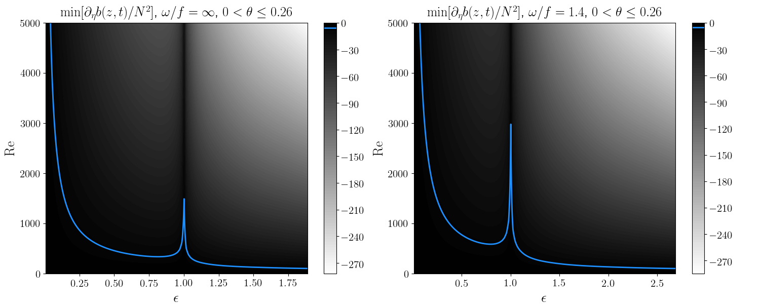
Figure 2: Total buoyancy gradient minima.

The minimum value (in both time and space) of the non-dimensional linear solution vertical buoyancy gradient for the non-rotating reference frame case ($f=0$, left)

and the rotating reference frame case (right).

4 Nonlinear solutions

In this section we examine the nonlinear stability and development of turbulence in boundary layers on smooth abyssal slopes for both rotating and non-rotating regimes. The boundary layers are initialized by the oscillating laminar flow solutions derived in Appendix A. We varied the slope Rossby number (nearly constant with slope, Equation 15), slope frequency ratio (Equation 14), Reynolds number (Equation 12), slope parameter (Equation 26), and slope angle $\theta$ for each of the 16 simulations as shown in table 1. The slope frequency ratio C and slope parameter $\epsilon$ are redundant for the non-rotating case, but are shown together because $\textit{C}\neq\epsilon$ for the rotating flow, and C appears explicitly in the forcing of the across-isobath ($x$) momentum equation. We observed bursts of turbulence, triggered by two-dimensional gravitational instabilities that rapidly become three-dimensional, during the upslope flow phase of all cases at $\Rey=840$ except for the lowest slope Burger number case, which exhibits turbulence sustained throughout the period. At $\Rey=420$ the flow matched the laminar analytical solutions except for weak turbulent bursts that occurred at the highest slope angles in the rotating regime.

Cases	Re	Ro	C	$\epsilon$	$\theta$ (rad)
1,9	840,420	$\infty$	0.25	0.25	3.53$\cdot 10^{-2}$
2,10	840,420	$\infty$	0.75	0.75	1.06$\cdot 10^{-1}$
3,11	840,420	$\infty$	1.25	1.25	1.76$\cdot 10^{-1}$
4,12	840,420	$\infty$	1.75	1.75	2.47$\cdot 10^{-1}$
5,13	840,420	1.41	0.25	0.35	3.53$\cdot 10^{-2}$
6,14	840,420	1.41	0.75	1.06	1.06$\cdot 10^{-1}$
7,15	840,420	1.43	1.25	1.79	1.76$\cdot 10^{-1}$
8,16	840,420	1.45	1.75	2.53	2.47$\cdot 10^{-1}$

Table 1: Non-dimensional simulation parameters.

The four independent parameters are $\Rey$, $\mathrm{Ro}$, C, $\theta$, and $\Pran=1$. The slope parameter $\epsilon=\tan\theta/\tan\theta_{c}$ is also used in this study to directly connect results to internal wave parameters. The slope Burger number is $\mathrm{Bu}={N^{2}\tan^{2}\theta}/f^{2}=\mathrm{Ro}^{2}\textit{C}^{2}$.

4.1 Numerical implementation

The flow anomalies, as defined by equations 34 and 35, are discretized to satisfy periodic boundary conditions in the wall parallel directions via Fourier spectral bases in the across-isobath ($x$) and along-isobath ($y$) directions. Periodicity is not merely numerically convienent; it also eliminates the need to prescribe buoyancy forcing (“restratification”) because the oscillating flow can advect the background field to gain or lose buoyancy. In the periodic domain, the boundary layer buoyancy can only reach a homogenized steady state if the turbulence sustainably converts tidal momentum to potential energy throughout the entire period.

Although the planar extent of the computational domain is less than the excursion length of the tide, the domain size (Table 2) is justifiably sufficient because the largest eddies in oscillating boundary layers are those associated with the transverse (wall normal) length scale, which is much less than the excursion length. Indeed, at higher Reynolds number ($\Rey=1790$), Gayen & Sarkar (2010b) found the turbulent boundary layer thickness, $\delta_{l}$, was $\delta_{l}=15\delta$ for the unstratified problem and $\delta_{l}=17\delta$ for flat plate stratified oscillating boundary layers at the same Reynolds number. The grid resolution parameters for the two Reynolds numbers examined are shown in Table 2, where ($L_{x},L_{y},H$) are the domain dimensions in ($x,y,z$), $l_{\text{K}}$ and $\tau_{\text{K}}$ are the Kolmogorov length and time scales, respectively, and wall units (denoted by ⁺) are scaled by the viscous length scale $\delta_{v}=\nu/U_{*}$ where $U_{*}$ is the a priori estimate of the friction velocity, which is approximated as $U_{*}=\sqrt{\nu\partial_{z}\overline{u}}\sim\sqrt{\nu{U_{\infty}}/{\delta}}$.

Solutions to the nonlinear anomaly equations,

$$\partial_{x}{u} +\partial_{y}{v}+\partial_{z}{w}=0,$$ (42)

$$\mathrm{d}_{t}{{u}} =\frac{1}{\textit{Ro}}{v}-\partial_{x}{p}+\frac{1}{\Rey_{L}}\big{(}\partial_{xx}+\partial_{yy}+\partial_{zz}\big{)}{u}+\textit{C}^{2}{b}+F(t)$$ (43)

$$\mathrm{d}_{t}{{v}} =-\frac{1}{\textit{Ro}}{u}-\partial_{y}{p}+\frac{1}{\Rey_{L}}\big{(}\partial_{xx}+\partial_{yy}+\partial_{zz}\big{)}{v},$$ (44)

$$\mathrm{d}_{t}{{w}} =-\partial_{z}{p}+\frac{1}{\Rey_{L}}\big{(}\partial_{xx}+\partial_{yy}+\partial_{zz}\big{)}{w}+\textit{C}^{2}{b}\cot\theta,$$ (45)

$$\mathrm{d}_{t}{{b}} =\frac{1}{\Pran\hskip 0.85358pt\Rey_{L}}\big{(}\partial_{xx}+\partial_{yy}+\partial_{zz}\big{)}{b},$$ (46)

where the anomalies $\mathrm{u},p$ and $b$ are defined by Equations 34-36, were computed using the MPI-parallel pseudo-spectral partial differential equation solver Dedalus (Burns et al. (2019)) using $128^{3}$ modes. A third-order, four-stage, implicit-explicit Runge-Kutta method derived by Ascher et al. (1997) was used for temporal integration. Chebyshev polynomial bases of the first kind were employed for spatial discretization on a cosine grid in the wall normal direction. Chebyshev polynomials permit the exact enforcement of the adiabatic wall boundary condition (Equation 28 minus the background component) on the buoyancy field and no-slip/impermeability wall boundary conditions on the velocities (Equation 27 minus the background component). The $3/2$ rule dealiasing scheme is used not only for dealiasing the spatial modes online but also for dealiasing post-processed flow statistics.

At the maximum wall normal extent of the domain, the boundary conditions at infinity (Equations 20, 21 and 29) were approximated for the anomalies as free-slip, impermeable conditions

$$\partial_{z}u=\partial_{z}v=w=0,$$ (47)

and an adiabatic condition on just the anomaly:

$$\partial_{z}b=0,$$ (48)

such that the total flow buoyancy gradient at the $z=H$ is the background buoyancy gradient in that direction.

Although the impermeability condition causes the reflection of internal waves that reach the upper boundary, the effects are assumed to be negligible because of the negligible amount of energy propagated by such high wavenumber waves in low Reynolds number flow. Gayen & Sarkar (2010a) found that for flat-bottomed stratified oscillatory flow at larger Reynolds number flow ($\Rey=1790$), the vertical wave energy flux is less than 1% of the boundary layer dissipation and production rates. Indeed, small but non-zero dissipation rates of turbulent kinetic energy were found near the upper boundary in some of the simulations, presumably from subharmonic parameteric instability or other wave-wave instabilities because of the free-slip reflective upper boundary condition. However, 99.9% of the shear production rate and dissipation rate occured within one Ozmidov length of the wall at the lower boundary for all simulations.

The initial conditions were specified as the sum of the steady component (Phillips (1970),Wunsch (1970)), the oscillating component (Thorpe (1987)) at time $t=0$, and uniformly distributed white noise corresponding to buoyancy anomaly perturbations of magnitude $10^{-10}$ m s^-2. All of the simulations that exhibited turbulence (defined as wall normal integrated production rates of turbulent kinetic energy greater than $10^{-10}$ m³ s^-3) did so within two oscillations.

The parameter regimes show in Table 1 qualitatively describe flows forced by the $M_{2}$ tide frequency, which is specified as $\omega=1.4\cdot 10^{-4}$ (rad s^-1, for a 12.4 hr tide period) and the Coriolis parameter is specified as is $f=10^{-4}$ (rad s^-1). Much of the abyssal ocean is filled with Antarctic Bottom Water (AABW), characterized by temperatures near $0^{\circ}{}$C and practical salinities of approximately 35 psu. At $0^{\circ}{}C$ and 35 psu, the kinematic viscosity is $1.83\times 10^{-6}$ m² s^-1 and the thermal diffusivity is $1.37\times 10^{-6}$ m² s^-1 (Chen et al. (1973), Talley (2011)). We specify the kinematic viscosity as $\nu=2\times 10^{-6}$ m² s^-1 and Pr$=1$. We approximate the background buoyancy frequency at mid latitude abyssal depths as $N=10^{-3}$ rad s^-1 (Thurnherr & Speer (2003)). Baroclinic tide amplitudes of $U_{\scalebox{0.9}{$\scriptscriptstyle\infty$}}\approx 1$ cm s^-1 are routinely observed near abyssal slopes (Simmons et al. (2004), Carter et al. (2008), Goff & Arbic (2010), Turnewitsch et al. (2013)) far from critical slopes, hydraulic spills, and other turbulence “hot spots.” Becker & Sandwell (2008) showed that the mean slopes lie between 0.00 and 0.10 over the vast majority of the seafloor below 2000 m, and that up to 15% of the slopes are super critical with respect to the M₂ tide.

Re	$L_{x}/\delta$,$L_{y}/\delta$	$H/\delta$	$\Delta{}x^{+},\Delta{}y^{+}$	$\Delta{}z^{+}_{\text{wall}}$	$\Delta{z}_{\text{wall}}/l_{\text{K}}$	$\Delta{t}_{\mathrm{d}}/\tau_{\text{K}}$	$\Delta{t}_{\mathrm{d}}/T$
420	59.3	177.8	9.5	0.69	0.40	0.01	$2.2\cdot 10^{-5}$
840	59.3	177.8	13.5	0.97	0.52	0.02	$2.2\cdot 10^{-5}$

Table 2: Simulation parameters

4.2 Intermittent turbulent bursts

The integrated turbulent kinetic energy (TKE) budget of each simulation was computed in order to distinguish the laminar and turbulent regimes and to quantify turbulence production mechanisms. The planar mean TKE is defined as

$$K(z,t)\equiv\frac{1}{2}\big{(}\overline{u^{\prime 2}}+\overline{v^{\prime 2}}+\overline{w^{\prime 2}}\big{)},$$ (49)

where the planar mean operator and variable decomposition are defined:

$$\overline{\phi}(z,t) =\frac{1}{L_{x}L_{y}}\int_{-L_{x}/2}^{L_{x}/2}\int_{-L_{y}/2}^{L_{y}/2}\phi(y,z,t)\hskip 2.84526pt\mathrm{dy}\hskip 2.84526pt\mathrm{dx},$$ (50)

$$\phi(x,y,z,t) =\overline{\phi}(z,t)+\phi^{\prime}(x,y,z,t),$$ (51)

and $\phi$ is any of the anomalous variables defined by Equations 34-36. The planar mean TKE evolution equation is

$${\partial_{t}{K}}+\partial_{z}\mathcal{T}=\mathcal{P}+\mathcal{B}-\varepsilon$$ (52)

The TKE transport term $\partial_{z}\mathcal{T}$ includes all TKE flux divergences (mean, turbulent, pressure, diffusion), which vanish upon wall normal integration of equation 52. The rate production of TKE by mean shear is $\mathcal{P}$ (production in the sense that, generally, $\mathcal{P}>0$), and it is defined as

$$\mathcal{P}(z,t) =-\overline{u^{\prime}w^{\prime}}\partial_{z}\overline{u}-\overline{v^{\prime}w^{\prime}}\partial_{z}\overline{v},$$ (53)

$$\mathcal{P}_{13} =-\overline{u^{\prime}w^{\prime}}\partial_{z}\overline{u},$$ (54)

$$\mathcal{P}_{23} =-\overline{v^{\prime}w^{\prime}}\partial_{z}\overline{v}.$$ (55)

The buoyancy flux $\mathcal{B}$ is typically downgradient ($\mathcal{B}<0$ amidst $\partial_{z}\overline{b}>0$ or $\mathcal{B}>0$ amidst $\partial_{z}\overline{b}<0$), in which case it represents the conversion of TKE into potential energy, and it is defined as

$$\mathcal{B}(z,t) =\overline{w_{\eta}^{\prime}b^{\prime}}=\overline{u^{\prime}b^{\prime}}\sin\theta+\overline{w^{\prime}b^{\prime}}\cos\theta,$$ (56)

$$\mathcal{B}_{1} =\overline{u^{\prime}b^{\prime}}\sin\theta,$$ (57)

$$\mathcal{B}_{3} =\overline{w^{\prime}b^{\prime}}\cos\theta,$$ (58)

in the rotated reference frame (where $w_{\eta}=\mathrm{d}_{t}\eta$ is the velocity in the vertical, not the wall normal velocity $w$). Defined in this manner a downgradient buoyancy flux may be reversible, so the term $\mathcal{B}$ includes both the turbulent stirring of and turbulent diffusion of buoyancy. A reversible buoyancy flux may be thought of as a buoyancy flux that converts turbulent kinetic energy into potential energy through stirring alone. Finally, the dissipation rate of turbulent kinetic energy,

$$\varepsilon(z,t)=\hskip 2.84526pt \nu\big{(}\overline{(\partial_{x}{u^{\prime}})^{2}}+\overline{(\partial_{x}{v^{\prime}})^{2}}+\overline{(\partial_{x}{w^{\prime}})^{2}}+\overline{(\partial_{y}{u^{\prime}})^{2}}+\overline{(\partial_{y}{v^{\prime}})^{2}}$$

$$+\overline{(\partial_{y}{w^{\prime}})^{2}}+\overline{(\partial_{z}{u^{\prime}})^{2}}+\overline{(\partial_{z}{v^{\prime}})^{2}}+\overline{(\partial_{z}{w^{\prime}})^{2}}\big{)}$$ (59)

is positive definite and therefore the last term of equation 52 is always a sink of TKE.

The oscillating boundary layer buoyancy gradient is transient and evanescent; therefore, we seek an integral quantity to measure the stabilizing/destabilizing effects of the buoyancy gradient. We borrow the concept of boundary layer displacement thickness (Monin & Yaglom (1971)) and apply it to buoyancy gradients rather than momentum. We refer to this measure as the boundary layer stratification thickness, $\delta_{s}$. If the total buoyancy field is not constant over small distance in the wall normal direction $z_{1}$, then it can be approximated as constant over some distance $z_{0}$ from the wall, where $z_{0}$ is defined by

$$N^{2}z_{0}=\int_{0}^{z_{1}}\partial_{z}\tilde{b}\hskip 2.84526pt\mathrm{dz}.$$ (60)

It follows that

$$\delta_{s}=z_{1}-z_{0}=\int_{0}^{z_{1}}\Big{(}1-\frac{\partial_{z}\tilde{b}}{N^{2}}\Big{)}\hskip 2.84526pt\mathrm{dz}.$$ (61)

$z_{1}$ can be chosen arbitrarily as a point outside the boundary layer because outside of the boundary layer $\partial_{z}\tilde{b}=N^{2}$ (the only non-zero buoyancy gradient component outside the boundary layer is the background hydrostatic component). Therefore, we set $z_{1}=H$ to calculate the stratification thickness.

The physical interpretation of Equation 60 is illustrated in Figure 3 as the calculation of the areas $\mathbf{A}_{1}$. $\delta_{s}>0$ and indicates that, in bulk, the boundary layer stratification is less than the background stratification, and vice versa. $\delta_{s}<0$ for both the laminar steady flow components because the analytical solutions (Phillips (1970),Wunsch (1970)) prescribe positive bulk stratification near the boundary where isopycnals curve downwards.

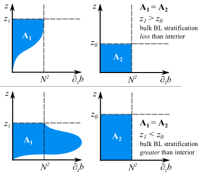
Figure 3: Stratification thickness concept.

The wave- and planar-averaged, wall normal integrated TKE budget statistics for $\Rey=840$ are shown in Figure 4. The statistics were wave averaged over 5-10 oscillations. All of the integrated TKE budgets at $\Rey=840$, with the exceptions of case 5 and arguably case 7, possess a single burst of chaotic three-dimensional motion that is characterized by a rapid increase in the production rate of the TKE from the across-slope shear, $\mathcal{P}_{13}$, the component of shear parallel to the direction of the oscillating body force. The turbulent bursts, which occur shortly after $t/T\approx 0.5$, preferentially select the phase regime during which the velocity is upslope but decelerating, the sign of the oscillating buoyancy changes from positive to negative, and the stratification thickness is negative (as indicated by the dark grey shading in Figure 4). The negative stratification thickness preference of the bursts contrasts the low Reynolds number, intermittent turbulence regime of Stokes’ second problem, in which a single burst occurs per oscillation, corresponding to the random selection of one of two shear maxima that occur within one period (Spalart & Baldwin (1987)).

To investigate the role of the linear buoyancy dynamics in the formation of the turbulent bursts in Figure 4, the time of the minimum total vertical buoyancy gradient in the linear solutions, which the reader may recall is negative for all of the considered parameter space as shown in figure 2, is depicted as the vertical dashed black line. The maximum TKE production rate by the mean shear approximately coincides in the time of the minimum total vertical buoyancy gradient for cases 1 and 6, the smallest intensity turbulent bursts shown in Figure 4. This result suggests that the bursts of TKE production rate by the mean shear are triggered by buoyant ejections of low momentum fluid upward. However, the triggering of buoyancy ejections is brief, weak, and not sustained, because the buoyancy fluxes in Figure 4 are negligible prior to bursts in the along-isobath shear production. Thus the gravitational instabilities appear to initiate, but not drive, bursts of chaotic three-dimensional motion.

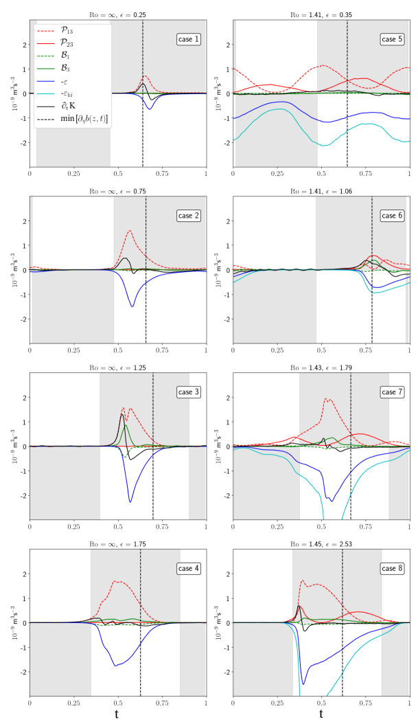
Figure 4: Wall-normal integrated, planar mean TKE budgets.

The gray shading corresponds to the sign of the stratification thickness (negative represents enhanced bulk boundary layer stratification, postive represents weakened and/or negative bulk boundary layer stratification. The dashed lines correspond to the time of the minimum total vertical buoyancy gradient in the linear solutions.

It is well known that boundary layer turbulence is inherently anisotropic. However, the majority of ocean turbulence measurements measure the fluctuations of the vertical shear of the horizontal velocities and then assume homogeneous isotropic turbulent motion to subsequently estimate the dissipation rate (Polzin & Montgomery (1996), St.Laurent et al. (2001)). The isotropic, homogeneous turbulence dissipation rate of TKE (Taylor (1935)) is defined in the sloped coordinate frame as

$$\varepsilon_{\text{hi}}=\frac{15}{4}\nu\cos^{2}\theta\big{(}\overline{(\partial_{z}u^{\prime})^{2}}+\overline{(\partial_{z}v^{\prime})^{2}}\big{)}.$$ (62)

The wall normal integrated form of $\varepsilon_{\mathrm{hi}}$ are plotted for the rotating reference frame cases in Figure 4 to illustrate that the assumptions of homogeneous anisotropic turbulence for near-wall abyssal flows may lead to overpredictions of the dissipation rate of TKE on the order of 100%, regardless of slope angle, even for the low Reynolds number boundary layers investigated here.

4.3 Gravitationally unstable rolls

Except for case 6, all of the simulations at $\Rey=840$ exhibited rolls characterized by growing streamwise vorticity. Figure 5 shows the instantaneous vertical velocity of case 2 to illustrate the life cycle of the rolls. In Figure 5, red corresponds to upward motions, and blue approximately corresponds to downward motions. The generation of two-dimensional convective rolls in the along-isobath / wall-normal ($y$-$z$) plane are visible just prior to the beginning of a burst. At time $t=0.51$ the rolls appear and by $t=0.55$ the rolls have begun to shear apart, erupting into the three-dimensional turbulence at the time of increase in TKE production by mean shear at $t=0.55$.

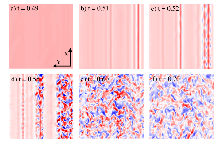
Figure 5: Contours of the vertical velocity, $w$, for case 2.

The contour plots show the vertical velocity at a fixed distance (roughly $\delta$) in the wall normal direction at six consecutive times. $w>0$ is colored red, while $w<0$ is colored blue. At $t=0.5$ the across-isobath velocity is positive but begins to decelerate. Simultaneously, two dimensional rolls form (see plot $b)$) in the $y-z$ plane, as heavier fluid is advected over lighter fluid trapped near the wall by the friction.

The rolls formed by gravitational instabilities in Figure 5 are qualitatively consistent with rolls observed in oscillating sloping stratified boundary layer experiments by Hart (1971). Hart (1971) identified spanwise plumes and rolls associated with the periodic reversals of the density gradient that qualitatively resembled the rolls that appeared in high Rayleigh number Couette flow experiments by Bénard & Avsec (1938), Chandra (1938), and Brunt (1951). Perhaps due to the similarity to the convection experiments, the rolls observed by Hart (1971) were referred to as “convective rolls.” Linear stability analyses by Deardorff (1965), Gallagher & A. Mercer (1965), and Ingersoll (1966), revealed that the growth of gravitationally unstable disturbances in high Rayleigh number Couette flows is suppressed in the plane of the shear (the streamwise-vertical plane) by the shear (i.e. the suppression of the spanwise vorticity disturbances). They also found that the growth of disturbances in the spanwise-vertical plane (steamwise vorticity disturbances) is unimpeded by the shear and grows in the same manner as pure convection. It has since been established that streamwise (the across-isobath direction) vortices with axes in the direction of a mean shear flow (a.k.a. “rolls”) can arise due to heating or centrifugal effects (Hu & Kelly (1997)). The initial growth of the rolls in Figure 5 appears to have similar attributes.

To verify the hypothesis that gravitational instabilities spawn the rolls, which in turn spawn the turbulent burst, an additional simulation with the same parameters as that of case 2, but with no nonlinear terms in the buoyancy equation, was executed. The simulation of the linearized buoyancy equation version of case 2 had no turbulent bursts over 10 cycles (all other simulations with bursts developed a burst within 2 cycles). The rolls are a bypass transition mechanism, lifting low momentum fluid up and bringing high momentum fluid down into the near wall flow, and so they transiently destabilize the shear. The transient gravitationally unstable buoyancy gradients, discussed previously, can trigger oscillating boundary layer turbulent bursts even if the buoyancy fluxes are a negligible source of TKE.

Although the streamwise rolls are initially two dimensional, they produce a three dimensional vorticity field. The inherent three dimensionality of the gravitational instability is evident in the Boussinesq baroclinic production of vorticity term ($\nabla\times{}\tilde{b}$) in the absolute vorticity budget for rotating and non-rotating oscillating boundary layers,

$$\text{baroclinic production}=\textit{C}^{2}\big{(}\overbrace{\partial_{y}\tilde{b}\cot\theta\mathbf{i}}^{\begin{subarray}{c}\text{nonlinear 2D rolls}\\ \vspace{0.5mm}\text{\& 3D bursts}\end{subarray}}+\hskip 7.11317pt(\overbrace{\partial_{x}\tilde{b}\cot\theta}^{\begin{subarray}{c}\text{nonlinear}\\ \vspace{0.5mm}\text{3D bursts}\end{subarray}}\hskip 5.69054pt-\overbrace{\partial_{z}\tilde{b}}^{\begin{subarray}{c}\text{linear flow}\\ \vspace{0.5mm}\text{\& 3D bursts}\end{subarray}})\mathbf{j}\hskip 11.38109pt-\overbrace{\partial_{y}\tilde{b}\mathbf{k}}^{\begin{subarray}{c}\text{nonlinear 2D rolls}\\ \vspace{0.5mm}\text{\& 3D bursts}\end{subarray}}\big{)}.$$ (63)

The linear OBL vorticity field has only one vorticity component, the spanwise vorticity in the $y$ direction, and the linear ROBL vorticity field is comprised of the spanwise vorticity and the streamwise vorticity in the $x$ direction. In either case, only the $\partial_{z}\tilde{b}\mathbf{j}$ term in Equation 63 is non-zero. However, the rolls produce gradients in the buoyancy field in the $y$ direction. The first and last terms on the righthand side of equation 63 indicate that the rolls in the $y-z$ plane will inevitably generate vorticity in the streamwise and wall normal directions; therefore, the rolls must induce three-dimensional motion in the oscillating boundary layers. Therefore the coherent structures shown in figure 5, which facilitate the transition to turbulence, must initiate secondary instabilities through three-dimensional baroclinic production of vorticity, a phenomenon that is widely observed in other stratified shear flow instabilities, e.g. Peltier & Caulfield (2003).

4.4 Relaminarization

During the phase of enhanced boundary layer stratification relative to the background, $\delta_{s}<0$ (the white regions in Figure 4), the boundary shear instabilities must overcome not only the stabilizing effect of increased stratification but also the stabilizing effect of the wall that is present regardless of phase. Linear stability analysis by Schlichting (1935) yielded a critical gradient Richardson number of 1/24 for a stratified Blasius boundary layer, notably lower than the Miles–Howard theorem threshold for inviscid stratified shear. This suggests that the flow is stabilized with respect to shear perturbations during $\delta_{s}<0$. However, if the flow is turbulent during the phase of $\delta_{s}<0$, the turbulence closure simulations for high Reynolds number by Umlauf & Burchard (2011) suggest mixing is much more efficient, presumably because the turbulence intensity required to overcome the strengthened boundary layer stratification must be considerable.

Three other mechanisms contribute to the relaminarization of the turbulent bursts in Figure 4. First, the turbulent burst diffuses the mean shear and thus its primary energy source. Second, the tidal acceleration opposes the mean shear during the second half of the phase, so the decay and reversal of the shear amplitude means that less mean flow kinetic energy is available. Third, once the flow reverses the outer boundary layer becomes increasingly stratified, as mentioned previously, when $\delta_{s}<0$. For a burst to persist across the entire period it must have a constant source of mean shear of large enough magnitude to sustain production of TKE throughout flow reversals and increased stratification.

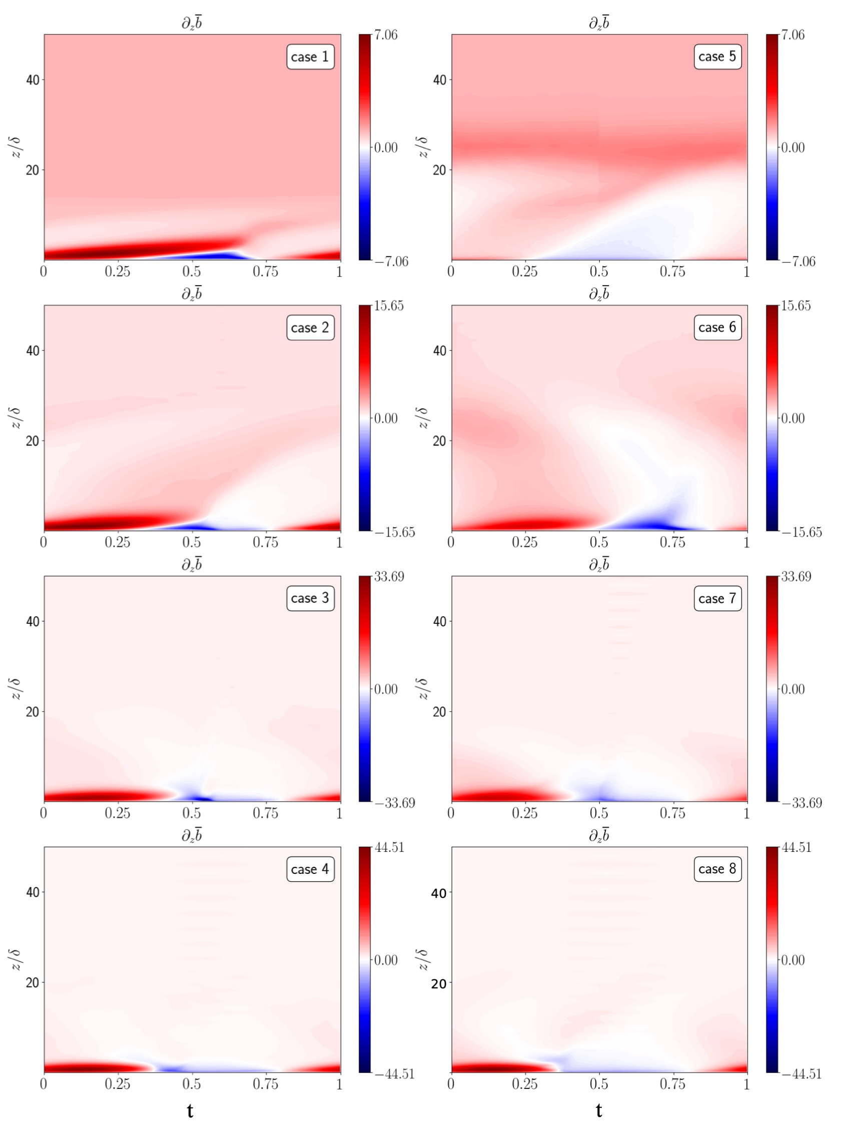
Figure 6: $\Rey=840$ Hövmuller plots of mean stratification.

The total wall normal buoyancy gradients are non-dimensionalized by $N^{2}$. The color bar axes show that the boundary layer stratification maxima/minima increase/decrease with increasing slope.

Case	Bu
5,13	0.124
6,14	1.127
7,15	3.173
8,16	6.347

Table 3: Rotating boundary layer simulation slope Burger numbers.

4.5 The effect of rotation

Only case 5 features sustained turbulence throughout the period (Figure 4) and sustained boundary layer buoyancy homogenization (Figure 6), because projection of the Coriolis force onto the wall normal direction increases with decreases slope. The Burger number is the ratio of the squares of the inertial period to the time scale associated with the buoyant restoring force. The slope Burger number accounts for the rotated reference frame, defined as

Bu $$=\textit{Ro}^{2}\textit{C}^{2}=\frac{N^{2}\tan^{2}\theta}{f^{2}}.$$ (64)

If Bu $<1$, the buoyant restoring force acts more slowly than the Coriolis force and rotation is significant. Table 3 shows the Burger number for the rotating boundary layer flows, cases 5–8 and 13–16. The lowest slope Burger number cases, 5 and 13, are influenced the most by rotation. In case 5, the highest Reynolds number and lowest Burger number flow, the turbulence is sustained throughout the period and the mean velocity field oscillates in a Stokes–Ekman layer manner. These results suggest that, within the investigated parameter regime, low Burger number flows are more likely to sustain turbulence throughout the entire period.

Case	Re	$c_{D}$
1,9	840,420	$1.8\cdot 10^{-4}$, $8.8\cdot 10^{-5}$
2,10	840,420	$9.7\cdot 10^{-4}$, $\sim 0$
3,11	840,420	$1.6\cdot 10^{-3}$, $\sim 0$
4,12	840,420	$3.5\cdot 10^{-3}$, $\sim 0$
5,13	840,420	$4.7\cdot 10^{-3}$, $\sim 0$
6,14	840,420	$5.1\cdot 10^{-4}$, $1.6\cdot 10^{-8}$
7,15	840,420	$5.0\cdot 10^{-3}$, $1.5\cdot 10^{-3}$
8,16	840,420	$5.4\cdot 10^{-3}$, $1.4\cdot 10^{-3}$

Table 4: Drag coefficients estimated from simulation time mean dissipation rates.

4.6 Barotropic tide dissipation

In oceanography, the rate of energy loss to drag per m² of the barotropic flow by tidal bottom boundary layers is often estimated using the quasi-empirical model $D\approx\rho_{0}c_{D}|U|U^{2}$ (Hoerner (1965)), where $c_{D}$ is the dimensionless drag coefficient and $U$ is an estimate of the bulk velocity (Jayne & St. Laurent (2001), St.Laurent & Garrett (2002)). The rate of energy dissipated by the tide can be represented in terms of Watts per meter squared by

$$D=\rho_{0}\int_{0}^{H}\overline{\varepsilon}\hskip 2.84526pt\mathrm{dz},$$ (65)

where $\overline{\varepsilon}$ is the dimensional time mean dissipation rate of TKE (units m²s^-3). For flat plate boundary layers, the transitional flow regime is characterized by drag coefficients in the range $0.001\leq{}c_{D}\leq 0.005$, for $1<\Rey<10^{3}$ or equivalently $1<\Rey_{L}<10^{6}$ (Hoerner (1965)). The drag coefficients for the low Reynolds number boundary layers in this study were calculated as

$$c_{D}=U_{\infty}^{-3}\int_{0}^{H}\overline{\varepsilon}\hskip 2.84526pt\mathrm{dz}.$$ (66)

The drag coefficients are shown in Table 4. The drag coefficient values shown in Table 4 mostly fall within the expected range for flat plate boundary layers, with the exception of the steepest slope case at $\Rey=840$, case 8. The drag coefficients are small at $\Rey=420$ for all but the steepest slope angles in the rotating reference frame (cases 15 and 16). In Table 4, $\sim 0$ represents negligible drag. The drag coefficients increase with slope at constant Reynolds number, and they effectively vanish somewhere in the range $420<\Rey<840$ on lower slopes where the flow is in the laminar or disturbed laminar regime.

5 Conclusions

We investigated transition pathways of low Reynolds number, oscillating, stratified, diffusive boundary layers on infinite slopes in both rotating and non-rotating reference frames. Our goal was to answer three questions regarding these flows within a non-dimensional parameter space qualitatively consistent with mid- and low-latitude $M_{2}$ tide boundary layers on smooth slopes:

1. How unstable are these boundary layers on typical abyssal slopes?
   Our results suggest that the laminar boundary layers are destabilized by a two-dimensional gravitational instability which rapidly progresses into three-dimensional motion and subsequently bursts of turbulence. This occurred for all of the investigated parameter space, except for at low slope Burger number (Bu$\leq 1/8$) and for low Reynolds number, low slope angle (Re$=$420, $\theta<0.1$) cases. The low slope Burger number, $\Rey\approx 840$, case is qualitatively similar to stratified Stokes-Ekman layers, and it was the only simulation that exhibited statistically stationary boundary layer buoyancy homogenization, or steady “mixing.” The low slope angle, low Reynolds number cases remained laminar.

   Vertically integrated TKE budgets suggest that energy supply to the turbulent bursts was extracted from the mean shear. Increasing the slope parameter $\epsilon$ resulted in increases in turbulent burst intensity, quantified by integrated TKE shear production, and also induced larger positive turbulent buoyancy fluxes. The positive turbulent buoyancy fluxes eroded negative buoyancy gradients and generated downgradient buoyancy diffusion. The turbulent bursts in rotating reference frames (slope $\mathrm{Ro}=1.4$) were qualitatively similar to the non-rotating reference frame bursts.

   During the phase of downslope mean flow the bursts where observed to relaminarize. With the exception of the low slope Burger number case, we observed that the boundary layer stratification significantly controls the transitional and intermittent regimes within $420\lesssim\Rey\lesssim 840$ by suppressing turbulence during the downslope flow phase and triggering TKE production by the mean shear during the upslope flow phase.

2. What are the instability mechanisms?
   Bulk estimates of the maximum boundary layer Rayleigh number (see Figure 2) from analytical solutions were consistent with gravitationally instabilities that were observed in direct numerical simulations of varying parameter space. The gravitational instabilities for rolls qualitatively resemble the convective rolls of diabatic Couette flow, and the correlation between the timing of their formation and gravitationally unstable stratfication in the boundary layer suggest that the instabilities are initiated by the upward ejection of buoyant low momentum fluid near the wall. Our results, the linear instability of diabatic Couette flow (Ingersoll (1966)), and Floquet linear instability of the laminar flow solutions (Kaiser (2020)), all suggest that the investigated flows are susceptible to graviational linear instability.

3. How valid are back-of-the-envelope barotropic tide dissipation rates?
   The dissipation rates of TKE and drag coefficients increased with increased slope parameter, more for the non-rotating cases than the rotating cases. The drag coefficients are negligible for $\Rey\approx 420$ flows, particularly on low angle slopes. The drag coefficients (Table 4) become quite small as the Reynolds number is decreased from 840 to 420, which suggests that a low tidal Reynolds number cutoff of $\Rey\approx 840$ is appropriate for barotropic tide drag parameterizations. The drag coefficients increased with slope angle although the steepest slopes in this study are not found in the ocean at large scales (scales equal to or greater than $k^{-1}$, the horizontal length scale of bathymetry).

6 Acknowledgements

B.K. was supported by a N.S.F. Graduate Research Fellowship and the Massachusetts Institute of Technology - Woods Hole Oceanographic Institution Joint Program, and by the National Science Foundation (OCE-1657870). The authors thank the Massachusetts Green Computing Center, Keaton Burns, Jesse Canfield, Raffaele Ferrari, Karl Helfrich, Kurt Polzin, Xiaozhou Ruan, and Andreas Thurnherr. This document is approved for Los Alamos Unlimited Release, LA-UR-21-28222.

Appendix A

The following is a derivation of the solutions to Equations 68, 69, and 70. In the other chapters of this thesis, partial derivatives are denoted by $\partial_{zz}$ for the second derivative in $z$, for example. In this appendix, Leibniz notation is used for derivatives. Begin by assuming linear oscillating solutions of the form

$$u_{\textrm{O},d}=\mathcal{U}(z)\mathrm{e}^{\text{i}\omega{t}},\quad v_{\textrm{O},d}=\mathcal{V}(z)\mathrm{e}^{\text{i}\omega{t}},\quad b_{\textrm{O},d}=\mathcal{B}(z)\text{ie}^{\text{i}\omega{t}},$$ (67)

where $d$ denotes the variables are dimensional and $\mathrm{O}$ denotes the oscillating components (Equations 30 and 32). It does not matter if we make the ansatz $\mathcal{V}(z)\mathrm{e}^{\text{i}\omega{t}}$ or $\mathcal{V}(z)\text{ie}^{\text{i}\omega{t}}$ (the latter is the correct final form) because the particular solution fixes the phase relationship of $u$ and $v$. The oscillating components of the dimensional and linearized forms of Equations 4-8, with no variation in the across-isobath ($x$) or along-isobath ($y$) directions, satisfy

$$\partial_{t}{{u}_{\textrm{O},d}} =f{v}_{\textrm{O},d}+\nu\partial_{zz}{u}_{\textrm{O},d}+{b}_{\textrm{O},d}\sin\theta+F_{d}(t)$$ (68)

$$\partial_{t}{{v}_{\textrm{O},d}} =-f{u}+\nu\partial_{zz}{v}_{\textrm{O},d},$$ (69)

$$\partial_{t}{{b}_{\textrm{O},d}} =-{u}_{\textrm{O},d}N^{2}\sin\theta+\kappa\partial_{zz}{b}_{\textrm{O},d},$$ (70)

where the wall normal momentum vanishes by conservation of mass, and the wall normal momentum equation again reduces to a diagnostic equation for the pressure field. Substitution of the ansatz (Equations 67) into the linearized governing equations 68, 69, and 70 yields

$$\Big{(}\text{i}\omega-\nu\frac{\partial^{2}}{\partial{z^{2}}}\Big{)}\mathcal{U}=\mathcal{V}f\cos\theta+{i}\mathcal{B}\sin\theta+Ai,$$ (71)

$$\Big{(}\text{i}\omega-\nu\frac{\partial^{2}}{\partial{z^{2}}}\Big{)}\mathcal{V}=-\mathcal{U}f\cos\theta,$$ (72)

$$\Big{(}\text{i}\omega-\kappa\frac{\partial^{2}}{\partial{z^{2}}}\Big{)}i\mathcal{B}=-\mathcal{U}N^{2}\sin\theta.$$ (73)

The equations above can be reduced to a single inhomogeneous linear partial differential equation for the wall-normal buoyancy structure $\mathcal{B}(z)$:

$$\Bigg{[}\Big{(}\text{i}\omega-\nu\frac{\partial^{2}}{\partial{z^{2}}}\Big{)}\Big{(}\text{i}\omega-\nu\frac{\partial^{2}}{\partial{z^{2}}}\Big{)}\Big{(}\text{i}\omega-\kappa\frac{\partial^{2}}{\partial{z^{2}}}\Big{)}+N^{2}\sin^{2}\theta\Big{(}\text{i}\omega-\nu\frac{\partial^{2}}{\partial{z^{2}}}\Big{)}$$

$$-f^{2}\cos^{2}\theta\Big{(}\text{i}\omega-\kappa\frac{\partial^{2}}{\partial{z^{2}}}\Big{)}\Bigg{]}i\mathcal{B}=A\omega{}N^{2}\sin\theta.$$ (74)

Equation 74 has six characteristic roots for the complementary (homogeneous) component of the solution and 6 linearly independent solutions. To obtain the characteristic solutions, expand all of the terms in Equation 74:

$$\Big{(}\frac{\partial^{6}}{\partial{z^{6}}}-i\Big{(}\frac{2\omega}{\nu}+\frac{\omega}{\kappa}\Big{)}\frac{\partial^{4}}{\partial{z^{4}}}+\Big{(}-\frac{\omega^{2}}{\nu^{2}}-\frac{2\omega^{2}}{\nu\kappa}+\frac{f^{2}\cos^{2}\theta{}}{\nu^{2}}+\frac{N^{2}\sin^{2}\theta{}}{\nu\kappa}\Big{)}\frac{\partial^{2}}{\partial{z^{2}}}$$

$$+i\Big{(}-\frac{f^{2}\cos^{2}\theta{}\omega}{\nu^{2}\kappa}-\frac{N^{2}\sin^{2}\theta{}\omega}{\nu^{2}\kappa}+\frac{\omega^{3}}{\nu^{2}\kappa}\Big{)}\Big{)}\mathcal{B}=i\frac{A\omega{}N^{2}\sin\theta}{\nu^{2}\kappa}$$ (75)

Therefore our the nonhomogeneous ordinary differential equation has the form:

$$\Big{(}\frac{\partial^{6}}{\partial{z^{6}}}+ia_{4}\frac{\partial^{4}}{\partial{z^{4}}}+a_{2}\frac{\partial^{2}}{\partial{z^{2}}}+ia_{0}\Big{)}\mathcal{B}=if_{p}$$ (76)

where the subscript $p$ denotes “particular solution” and

$$a_{4} =-\Big{(}\frac{2\omega}{\nu}+\frac{\omega}{\kappa}\Big{)}=-\frac{\omega}{\kappa}\Big{(}\frac{2}{\Pran}+1\Big{)}=-\frac{\omega}{\kappa}\Big{(}\frac{2+\Pran}{\Pran}\Big{)}$$

$$a_{2} =-\frac{\omega^{2}}{\nu^{2}}-\frac{2\omega^{2}}{\nu\kappa}+\frac{f^{2}\cos^{2}\theta{}}{\nu^{2}}+\frac{N^{2}\sin^{2}\theta{}}{\nu\kappa}=\frac{f^{2}\cos^{2}\theta{}+\Pran N^{2}\sin^{2}\theta{}-\omega^{2}(1+2\Pran)}{\kappa^{2}\Pran^{2}}$$

$$a_{0} =\frac{\omega^{3}}{\nu^{2}\kappa}-\frac{f^{2}\cos^{2}\theta{}\omega}{\nu^{2}\kappa}-\frac{N^{2}\sin^{2}\theta{}\omega}{\nu^{2}\kappa}=\frac{\omega(\omega^{2}-f^{2}\cos^{2}\theta{}-N^{2}\sin^{2}\theta{})}{\kappa^{3}\Pran}$$

$$f_{p} =\frac{A\omega{}N^{2}\sin\theta}{\nu^{2}\kappa}$$ (77)

Equation 76 has the characteristic equation:

$$\lambda^{6}+ia_{4}\lambda^{4}+a_{2}\lambda^{2}+ia_{0}=0,$$ (78)

which has 6 distinct solutions for $\lambda$. The total general solution is the sum of the complementary (homogeneous) solutions and the particular (nonhomogeneous) solutions:

$$\mathcal{B}(z)=\mathcal{B}_{\textit{C}}(z)+\mathcal{B}_{\text{p}}(z)$$ (79)

The complementary solution is therefore of the form:

$$\mathcal{B}_{\textit{C}}(z)=c_{1}\mathrm{e}^{\lambda_{1}}+c_{2}\mathrm{e}^{\lambda_{2}}+c_{3}\mathrm{e}^{\lambda_{3}}+c_{4}\mathrm{e}^{\lambda_{4}}+c_{5}\mathrm{e}^{\lambda_{5}}+c_{6}\mathrm{e}^{\lambda_{6}}$$ (80)

and the particular part of the solution is of the form:

$$\mathcal{B}_{\text{p}}=a_{p}$$ (81)

where $a_{p}$ is an unknown constant.

A.1 The particular solution

To solve for $a_{p}$, substitute the particular solution form (Equation 81 into the nonhomogeneous governing equation (Equation 76):

$$a_{p} =\frac{f_{p}}{a_{0}}$$

$$=\frac{AN^{2}\sin\theta}{\omega^{2}-f^{2}\cos^{2}\theta{}-N^{2}\sin^{2}\theta{}}$$ (82)

The complementary solution

Let $\phi=\lambda^{2}$ in Equation 78 to obtain:

$$\phi^{3}+ia_{4}\phi^{2}+a_{2}\phi+ia_{0}=0,$$ (83)

where

$$\lambda_{1,2}=\pm\sqrt{\phi_{1}},\qquad\lambda_{3,4}=\pm\sqrt{\phi_{2}},\qquad\lambda_{5,6}=\pm\sqrt{\phi_{2}},$$ (84)

The solutions to this equation are:

$$\beta=\sqrt[3]{2ia_{4}^{3}+9ia_{2}a_{4}+3\sqrt{3}\sqrt{4a_{2}^{3}+a_{4}^{2}a_{2}^{2}+18a_{0}a_{4}a_{2}+4a_{0}a_{4}^{3}-27a_{0}^{2}}-27ia_{0}}$$ (85)

$$\phi_{1}=\frac{\beta}{3\sqrt[3]{2}}-\frac{\sqrt[3]{2}\left(a_{4}^{2}+3a_{2}\right)}{3\beta}-\frac{ia_{4}}{3}$$ (86)

$$\phi_{2}=-\frac{\left(1-i\sqrt{3}\right)\beta}{6\sqrt[3]{2}}+\frac{\left(1+i\sqrt{3}\right)\left(a_{4}^{2}+3a_{2}\right)}{3\cdot 2^{2/3}\beta}-\frac{ia_{4}}{3}$$ (87)

$$\phi_{3}=-\frac{\left(1+i\sqrt{3}\right)\beta}{6\sqrt[3]{2}}+\frac{\left(1-i\sqrt{3}\right)\left(a_{4}^{2}+3a_{2}\right)}{3\cdot 4^{1/3}\beta}-\frac{ia_{4}}{3}$$ (88)

A.2 Boundary conditions

For the parameter space we are interested in $c_{1}=c_{3}=c_{5}=0$ (to have finite solutions at $z=\infty$):

$$\mathcal{B}(z)=c_{2}\mathrm{e}^{-\sqrt{\phi_{1}}z}+c_{4}\mathrm{e}^{-\sqrt{\phi_{2}}z}+c_{6}\mathrm{e}^{-\sqrt{\phi_{3}}z}+a_{p}$$ (89)

Now we reinterpret the boundary conditions in terms of $\mathcal{B}$:

1. No-slip at the wall ($z=0$) applied to the across slope velocity

   $$\mathcal{U}=-\frac{1}{N^{2}\sin\theta}\Big{(}\text{i}\omega-\kappa\frac{\partial^{2}}{\partial{z^{2}}}\Big{)}i\mathcal{B}=0,$$

   leads to the expression:

   $$c_{2}(\omega+i\kappa\phi_{1})+c_{4}(\omega+i\kappa\phi_{2})+c_{6}(\omega+i\kappa\phi_{3})=-a_{p}\omega$$ (90)

2. No-slip at the wall ($z=0$) applied to the along slope velocity

   $$\mathcal{V}=\frac{1}{f\cos\theta}\Big{(}\frac{1}{N^{2}\sin\theta}\Big{(}\omega^{2}+\text{i}\omega(\nu+\kappa)\frac{\partial^{2}}{\partial{z^{2}}}-\nu\kappa\frac{\partial^{4}}{\partial{z^{4}}}\Big{)}\mathcal{B}-\sin\theta\mathcal{B}-A\Big{)}=0,$$

   leads to the expression:

   $$c_{6}(\text{i}\omega\phi_{3}(\kappa+\nu)-\kappa\nu\phi_{3}^{2}-N^{2}\sin^{2}\theta+\omega^{2})+$$

   $$c_{2}\left(i\omega\phi_{1}(\kappa+\nu)-\kappa\nu\phi_{1}^{2}-N^{2}\sin^{2}\theta+\omega^{2}\right)+$$

   $$c_{4}\left(i\omega\phi_{2}(\kappa+\nu)-\kappa\nu\phi_{2}^{2}-N^{2}\sin^{2}\theta+\omega^{2}\right)=AN^{2}\sin\theta-a_{p}\left(\omega^{2}-N^{2}\sin^{2}\theta\right)$$ (91)

3. The adiabatic wall boundary condition

   $$\frac{\partial\mathcal{B}}{\partial{z}}=0+0i\quad\text{at}\quad z=0$$

   leads to the expression:

   $$-c_{4}\sqrt{\phi_{2}}-c_{6}\sqrt{\phi_{3}}-c_{2}\sqrt{\phi_{1}}=0$$ (92)

Therefore we can solve for the coefficients: In matrix form:

$$\mathbf{E}\cdot\mathbf{x}=\mathbf{y}$$

or

$$\begin{bmatrix}E_{11}&E_{12}&E_{13}\\ E_{21}&E_{22}&E_{23}\\ E_{31}&E_{32}&E_{33}\end{bmatrix}\begin{bmatrix}x_{1}\\ x_{2}\\ x_{3}\end{bmatrix}=\begin{bmatrix}y_{1}\\ y_{2}\\ y_{3}\\ \end{bmatrix}$$ (93)

where we solve for

$$x_{1}=c_{2}=b_{1},\quad x_{2}=c_{4}=b_{2},\quad x_{3}=c_{6}=b_{3},$$ (94)

with $\mathbf{E}$ and $\mathbf{y}$ specified the boundary conditions:

$$y_{1}=-a_{p}\omega{},\quad y_{2}=AN^{2}\sin\theta-a_{p}\left(\omega^{2}-N^{2}\sin^{2}\theta\right),\quad y_{3}=0,$$

$$E_{11}=\omega+i\kappa\phi_{1},\quad E_{12}=\omega+i\kappa\phi_{2},\quad E_{13}=\omega+i\kappa\phi_{3},$$

$$E_{21}=i\omega\phi_{1}(\kappa+\nu)-\kappa\nu\phi_{1}^{2}-N^{2}\sin^{2}\theta+\omega^{2},$$

$$E_{22}=i\omega\phi_{2}(\kappa+\nu)-\kappa\nu\phi_{2}^{2}-N^{2}\sin^{2}\theta+\omega^{2},$$

$$E_{23}=\text{i}\omega\phi_{3}(\kappa+\nu)-\kappa\nu\phi_{3}^{2}-N^{2}\sin^{2}\theta+\omega^{2},$$

$$E_{31}=-\sqrt{\phi_{1}},\quad E_{32}=-\sqrt{\phi_{2}},\quad E_{33}=-\sqrt{\phi_{3}},$$

The solutions for the coefficients in the $\mathcal{B}$ solution (see Equation 94) are:

$$\Upsilon =\kappa^{2}\nu(\sqrt{\phi_{2}\phi_{3}}\phi_{1}+\sqrt{\phi_{1}\phi_{3}}\phi_{2}+\sqrt{\phi_{1}\phi_{2}}\phi_{3})$$

$$+i\kappa\nu\omega(\sqrt{\phi_{1}\phi_{2}}+\sqrt{\phi_{1}\phi_{3}}+\sqrt{\phi_{2}\phi_{3}}+\phi_{1}+\phi_{2}+\phi_{3})$$

$$+\nu\omega^{2}+\kappa N^{2}\sin^{2}\theta,$$

$$b_{1} =-\frac{1}{\left(\sqrt{\phi_{1}}-\sqrt{\phi_{2}}\right)\left(\sqrt{\phi_{1}}-\sqrt{\phi_{3}}\right)\Upsilon}\big{(}A\kappa N^{2}\sqrt{\phi_{2}\phi_{3}}\sin\theta+iAN^{2}\omega\sin\theta+\kappa N^{2}a_{p}\sqrt{\phi_{2}\phi_{3}}\sin^{2}\theta$$

$$+i\kappa\nu a_{p}\omega(\sqrt{\phi_{3}}\phi_{2}^{3/2}+\phi_{3}\phi_{2}+\sqrt{\phi_{2}}\phi_{3}^{3/2})+\nu a_{p}\omega^{2}\sqrt{\phi_{2}\phi_{3}}\big{)}$$ (95)

$$b_{2} =\frac{1}{\left(\sqrt{\phi_{1}}-\sqrt{\phi_{2}}\right)\left(\sqrt{\phi_{2}}-\sqrt{\phi_{3}}\right)\Upsilon}\Big{(}A\kappa N^{2}\sqrt{\phi_{1}\phi_{3}}\sin\theta+iAN^{2}\omega\sin\theta+\kappa N^{2}a_{p}\sqrt{\phi_{1}\phi_{3}}\sin^{2}\theta$$ (96)

$$+i\kappa\nu a_{p}\omega(\sqrt{\phi_{3}}\phi_{1}^{3/2}+\phi_{3}\phi_{1}+\sqrt{\phi_{1}}\phi_{3}^{3/2})+\nu a_{p}\omega^{2}\sqrt{\phi_{1}\phi_{3}}\Big{)}$$

$$b_{3} =-\frac{1}{\left(\sqrt{\phi_{1}}-\sqrt{\phi_{3}}\right)\left(\sqrt{\phi_{2}}-\sqrt{\phi_{3}}\right)\Upsilon}\Big{(}A\kappa N^{2}\sqrt{\phi_{1}\phi_{2}}\sin\theta+iAN^{2}\omega\sin\theta+\kappa N^{2}a_{p}\sqrt{\phi_{1}\phi_{2}}\sin^{2}\theta$$ (97)

$$+\text{i}\kappa\nu a_{p}\omega(\sqrt{\phi_{2}}\phi_{1}^{3/2}+\phi_{2}\phi_{1}+\sqrt{\phi_{1}}\phi_{2}^{3/2})+\nu a_{p}\omega^{2}\sqrt{\phi_{1}\phi_{2}}\Big{)}$$

A.3 Solutions

The solutions for the oscillating component of the flow (the components with subscript “O” in Equations 30 and 31)

$$b_{\textrm{O},d}(z,t)=\Real\big{[}\mathcal{B}(z)\text{ie}^{\text{i}\omega{t}}\big{]}=\Real\big{[}\big{(}c_{2}\mathrm{e}^{-\sqrt{\phi_{1}}z}+c_{4}\mathrm{e}^{-\sqrt{\phi_{2}}z}+c_{6}\mathrm{e}^{-\sqrt{\phi_{3}}z}+a_{p}\big{)}\text{ie}^{\text{i}\omega{t}}\big{]}$$ (98)

where $b_{1},b_{2},$ and $b_{3}$ are given by Equations 95, 96, and 97. The across-slope velocity coefficients are:

$$u_{1} =b_{1}(\omega+\text{i}\kappa\phi_{1}),$$ (99)

$$u_{2} =b_{2}(\omega+\text{i}\kappa\phi_{2}),$$ (100)

$$u_{3} =b_{3}(\omega+\text{i}\kappa\phi_{3}),$$ (101)

and the along-slope velocity coefficients are:

$$v_{1} =b_{1}(\text{i}\omega\phi_{1}(\kappa+\nu)-\kappa\nu\phi_{1}^{2}-N^{2}\sin^{2}\theta+\omega^{2}),$$ (102)

$$v_{2} =b_{2}(\text{i}\omega\phi_{2}(\kappa+\nu)-\kappa\nu\phi_{2}^{2}-N^{2}\sin^{2}\theta+\omega^{2}),$$ (103)

$$v_{3} =b_{3}(\text{i}\omega\phi_{3}(\kappa+\nu)-\kappa\nu\phi_{3}^{2}-N^{2}\sin^{2}\theta+\omega^{2}),$$ (104)

and the velocity solutions are

$$u_{\textrm{O},d}(z,t) =\Real\big{[}\mathcal{U}(z)\mathrm{e}^{\text{i}\omega{t}}\big{]}$$ (105)

$$=\Real\Big{[}\frac{\big{(}u_{1}\mathrm{e}^{-\sqrt{\phi_{1}}z}+u_{2}\mathrm{e}^{-\sqrt{\phi_{2}}z}+u_{3}\mathrm{e}^{-\sqrt{\phi_{3}}z}+a_{p}\omega\big{)}\mathrm{e}^{\text{i}\omega{t}}}{N^{2}\sin\theta}\Big{]}$$

$$v_{\textrm{O},d}(z,t) =\Real\big{[}\mathcal{V}(z)\text{ie}^{\text{i}\omega{t}}\big{]}$$ (106)

$$=\Real\Big{[}\frac{\big{(}v_{1}\mathrm{e}^{-\sqrt{\phi_{1}}z}+v_{2}\mathrm{e}^{-\sqrt{\phi_{2}}z}+v_{3}\mathrm{e}^{-\sqrt{\phi_{3}}z}+a_{p}(\omega^{2}-N^{2}\sin^{2}\theta)-AN^{2}\sin\theta\big{)}\text{ie}^{\text{i}\omega{t}}}{fN^{2}\cos\theta\sin\theta}\Big{]}$$

References

- Ascher et al. (1997) Ascher, U., Ruuth, S. & Spiteri, R. 1997 Implicit-explicit runge-kutta methods for time-dependent partial differential equations. Applied Numerical Mathematics 25 (2), 151–167.
- Balmforth et al. (2002) Balmforth, N., Ierley, G. & Young, W. 2002 Tidal conversion by subcritical topography. Journal of Physical Oceanography 32 (10), 2900–2914.
- Becker & Sandwell (2008) Becker, J. & Sandwell, D. 2008 Global estimates of seafloor slope from single-beam ship soundings. Journal of Geophysical Research: Oceans 113 (C5).
- Bell (1975a) Bell, T. 1975a Lee waves in stratified flows with simple harmonic time dependence. Journal of Fluid Mechanics 67, 705–722.
- Bell (1975b) Bell, T. 1975b Topographically generated internal waves in the open ocean. Journal of Geophysical Research 80, 320–327.
- Bénard & Avsec (1938) Bénard, H. & Avsec, D. 1938 Travaux récents sur les tourbillons cellulaires et les tourbillons en bandes. applications à l’astrophysique et à la météorologie. J. Phys. Radium 9 (11), 486–500.
- Brunt (1951) Brunt, D. 1951 Experimental cloud formation. In Compendium of Meteorology, pp. 1255–1262. Springer.
- Burns et al. (2019) Burns, K., Vasil, G., Oishi, J., Lecoanet, D. & Brown, B. 2019 Dedalus: A flexible framework for numerical simulations with spectral methods. arXiv preprint arXiv:1905.10388 .
- Carter et al. (2008) Carter, G., Merrifield, M., Becker, J., Katsumata, K., Gregg, M., Luther, D., Levine, M., Boyd, T. & Firing, Y. 2008 Energetics of m 2 barotropic-to-baroclinic tidal conversion at the hawaiian islands. Journal of Physical Oceanography 38 (10), 2205–2223.
- Chandra (1938) Chandra, K. 1938 Instability of fluids heated from below. Proceedings of the Royal Society of London. Series A-Mathematical and Physical Sciences 164 (917), 231–242.
- Chandrasekhar (1961) Chandrasekhar, S. 1961 Hydrodynamic and hydromagnetic stability. Oxford University Press.
- Chen et al. (1973) Chen, S., Chan, R., Read, S. & Bromley, L. 1973 Viscosity of sea water solutions. Desalination 13 (1), 37–51.
- Davis (1976) Davis, S. 1976 The stability of time-periodic flows. Annual Review of Fluid Mechanics 8 (1), 57–74.
- Deardorff (1965) Deardorff, J. 1965 Gravitational instability between horizontal plates with shear. The Physics of Fluids 8 (6), 1027–1030.
- Ferrari et al. (2016) Ferrari, R., Mashayek, A., McDougall, T., Nikurashin, M. & Campin, J. 2016 Turning ocean mixing upside down. Journal of Physical Oceanography .
- Gallagher & A. Mercer (1965) Gallagher, A. & A. Mercer, A McD 1965 On the behaviour of small disturbances in plane couette flow with a temperature gradient. Proceedings of the Royal Society of London. Series A. Mathematical and Physical Sciences 286 (1404), 117–128.
- Garrett & Kunze (2007) Garrett, C. & Kunze, E. 2007 Internal tide generation in the deep ocean. Annual Review of Fluid Mechanics 39, 57–87.
- Gayen & Sarkar (2010a) Gayen, B. & Sarkar, S. 2010a Large eddy simulation of a stratified boundary layer under an oscillatory current. Journal of Fluid Mechanics 643, 233–266.
- Gayen & Sarkar (2010b) Gayen, B. & Sarkar, S. 2010b Turbulence during the generation of internal tide on a critical slope. Physical Review Letters 104 (21).
- Goff & Arbic (2010) Goff, J. & Arbic, B. 2010 Global prediction of abyssal hill roughness statistics for use in ocean models from digital maps of paleo-spreading rate, paleo-ridge orientation, and sediment thickness. Ocean Modelling 32 (1), 36–43.
- Hart (1971) Hart, J. 1971 A possible mechanism for boundary layer mixing and layer formation in a stratified fluid. Journal of Physical Oceanography 1, 258–262.
- Hoerner (1965) Hoerner, S. 1965 Fluid-dynamic drag. Hoerner fluid dynamics .
- Hu & Kelly (1997) Hu, H. & Kelly, R. 1997 Stabilization of longitudinal vortex instabilities by means of transverse flow oscillations. Physics of Fluids 9 (3), 648–654.
- Ingersoll (1966) Ingersoll, A. 1966 Convective instabilities in plane couette flow. The Physics of Fluids 9 (4), 682–689.
- Jayne & St. Laurent (2001) Jayne, S. & St. Laurent, L. 2001 Parameterizing tidal dissipation over rough topography. Geophysical Research Letters 28 (5), 811–814.
- Kaiser (2020) Kaiser, Bryan Edward 2020 Finescale abyssal turbulence: sources and modeling. PhD thesis, Massachusetts Institute of Technology.
- Monin & Yaglom (1971) Monin, A. & Yaglom, A. 1971 Statistical fluid dynamics, , vol. 1. MIT Press.
- Peltier & Caulfield (2003) Peltier, W. & Caulfield, C. 2003 Mixing efficiency in stratified shear flows. Annual Review of Fluid Mechanics 35 (1), 135–167.
- Phillips (1970) Phillips, O. 1970 On flows induced by diffusion in a stably stratified fluid. Deep Sea Research and Oceanographic Abstracts 17 (3), 435–443.
- Polzin (1996) Polzin, K. 1996 Statistics of the richardson number: Mixing models and finestructure. Journal of physical oceanography 26 (8), 1409–1425.
- Polzin & Montgomery (1996) Polzin, K. & Montgomery, E. 1996 Microstructure profiling with the high resolution profiler. Proceedings of the Office of Naval Research Workshop on Microstructure Sensors pp. 109–115.
- Sarkar & Scotti (2017) Sarkar, S. & Scotti, A. 2017 From topographic internal gravity waves to turbulence. Annual Review of Fluid Mechanics 49, 195–220.
- Schlichting (1935) Schlichting, H. 1935 Hauptaufsätze: turbulenz bei wärmeschichtung. ZAMM Journal of Applied Mathematics and Mechanics 15 (6), 313–338.
- Simmons et al. (2004) Simmons, H., Hallberg, R. & Arbic, B. 2004 Internal wave generation in a global baroclinic tide model. Deep Sea Research Part II: Topical Studies in Oceanography 51 (25-26), 3043–3068.
- Spalart & Baldwin (1987) Spalart, P. & Baldwin, B. 1987 Direct simulation of a turbulent oscillating boundary layer. In Turbulent shear flows 6, pp. 417–440. Springer.
- St.Laurent & Garrett (2002) St.Laurent, L. & Garrett, C. 2002 The role of internal tides in mixing the deep ocean. Journal of Physical Oceanography 32 (10), 2882–2899.
- St.Laurent et al. (2001) St.Laurent, L., Toole, J. & Schmitt, R. 2001 Buoyancy forcing by turbulence above rough topography in the abyssal brazil basin. Journal of Physical Oceanography 31 (12), 3476–3495.
- Talley (2011) Talley, L. 2011 Descriptive Physical Oceanography. Academic Press.
- Taylor (1935) Taylor, G. 1935 Statistical theory of turbulence. Proceedings of the Royal Society of London. Series A, Mathematical and Physical Sciences 151 (873), 421–444.
- Thorpe (1987) Thorpe, S. 1987 Current and temperature variability on the continental slope. Philosophical Transactions of the Royal Society of London A: Mathematical, Physical and Engineering Sciences 323, 471–517.
- Thurnherr & Speer (2003) Thurnherr, A. & Speer, K. 2003 Boundary mixing and topographic blocking on the mid-atlantic ridge in the south atlantic. Journal of Physical Oceanography 33 (4), 848–862.
- Turnewitsch et al. (2013) Turnewitsch, R., Falahat, S., Nycander, J., Dale, A., Scott, R. & Furnival, D. 2013 Deep-sea fluid and sediment dynamics—influence of hill-to seamount-scale seafloor topography. Earth-Science Reviews 127, 203–241.
- Umlauf & Burchard (2011) Umlauf, L. & Burchard, H. 2011 Diapycnal transport and mixing efficiency in stratified boundary layers near sloping topography. Journal of Physical Oceanography 41 (2), 329–345.
- Wunsch (1970) Wunsch, C. 1970 On oceanic boundary mixing. Deep Sea Research and Oceanographic Abstracts 17 (2), 293–301.
- Zilberman et al. (2009) Zilberman, N., Becker, J., Merrifield, M. & Carter, G. 2009 Model estimates of m 2 internal tide generation over mid-atlantic ridge topography. Journal of Physical Oceanography 39 (10), 2635–2651.