Detecting Confined and Deconfined Spinons in Dynamical Quantum Simulations

Abstract

Dynamical spin-structure factor (DSF) contains fingerprint information of collective excitations in interacting quantum spin systems. In solid state experiments, DSF can be measured through neutron scatterings. However, it is in general challenging to compute the spectral properties accurately via many-body simulations. Currently, quantum simulation and computation constitute a thriving research field, which are believed to provide a very promising platform for simulating quantum many-body systems. In this work, we establish a link between the many-body dynamics and quantum simulations by studying the non-equilibrium DSF (nDSF) measured on direct product states, which are accessible in contemporary quantum simulators with Rydberg atoms, superconducting qubits, etc. Based on the many-body calculations of transverse field Ising chains, we find the nDSF can be used to sensitively probe the multi-spinon continua associated with the two-spinon creation and the spinon-antispinon process, etc. Moreover, we further demonstrate that the low-energy spinons can be confined — forming spinon bound states — under a finite longitudinal field. Our results pave the way of quantum simulation and manipulation of fractional excitations in highly-entangled quantum many-body systems.

I Introduction

Hunting exotic quasi-particles in ultra quantum states of matter constitutes a fundamental research topic in modern condensed matter and quantum physics. One prominent example is the fractional spinon in one-dimensional (1D) spin chain, which is a charge neutral quasi-particle carrying fractional spin quantum number [1]. Intuitively, the spinon excitation in a quantum Ising chain can be regarded as the domain wall moving freely in Fig. 1, which has been evidenced experimentally in spin-chain compounds via the inelastic neutron scattering measurements [2, 3, 4]. Despite the existence of well-recognised model materials like the spin-1/2 Heisenberg chain compound KCuF₃ [2], Ising-chain material CoNb₂O₆ [5, 6, 7, 8], the rare-earth Heisenberg XXZ chain Yb₂Pt₂Pb [4, 9], YbAlO₃ [10], etc, there inevitably exist additional interactions in solid-state compounds beyond the “clean" models. It thus adds complexity in the analysis of the exotic excitations in these quantum magnets.

On the other hand, simulations of the dynamical spin structure factor (DSF) are quite challenging in many-body calculations. Dynamical exact diagonalization suffers from strong finite-size effects, the quantum Monte Carlo methods have essential difficulties in dealing with real-time dynamics, and the matrix product state (MPS) based simulations do not have the access to long-time dynamics due to the rapid entanglement growth and thus the obtained spectral properties have rather limited resolution in frequencies. Therefore, to study the long-time dynamics of many-body systems we need to seek for different tools.

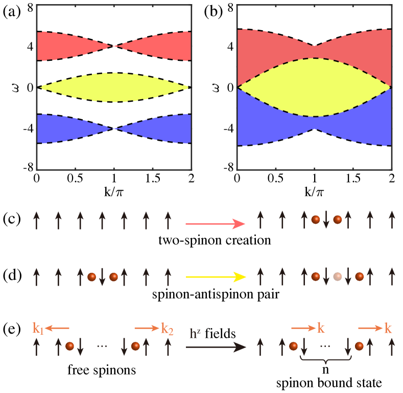
Figure 1: (a) shows the bowtie- and shell-shape spin excitation continua present in the gapped phases of the TFI model, and (b) depicts the excitation continua right at the QCP, where the lower boundary of the bowtie excitations coincides with that of the upper boundary of the shell excitations. The cartoon pictures of the (c) two-spinon creation and (d) spinon-antispinon processes are illustrated, which are responsible for the bowtie and shell excitation continua. All these spinon continua are determined by $\omega(k)=\pm\epsilon(k_{1})\pm\epsilon(k_{2})$, where $k=k_{1}+k_{2}$ and $\pm\epsilon(k)$ is the spinon ($+$) or antispinon ($-$) dispersion. The single-spinon dispersions used in the illustration are $\epsilon(k)\simeq 2-\sin(2\gamma)\cos k$ (away from QCP) and $\epsilon(k)=2\sqrt{2}\left|\sin\left(\frac{k}{2}\right)\right|$ (right at QCP). (e) Confinement of spinons under nonzero longitudinal fields, where the bound states consist of two spinons at a distance $n=1,2,\cdots$ and move at the same quasi-momentum $k$.

The rapid development of quantum technologies in past few years has witnessed the dawn of the quantum era [11, 12, 13, 14], and offers unique access to long-time evolution of quantum systems. Although the universal quantum computing is still quite far from reach at the current moment, the idea of quantum simulation, i.e., emulating the problem to be solved via a highly controllable quantum system, is gradually becoming reality, which would fundamentally reformulate the routine that scientists conquer the uncharted territory of the realm of nature in the future [15]. In particular, physicists are making increasing endeavor to design quantum simulation protocols to solve many important problems in diverse fields of physics, ranging from lattice gauge theory [16], Kibble-Zurich mechanism [17], many-body localization [18, 19, 20, 21], phase diagram of Hubbard model [22, 23, 24, 25, 26] to quantum walk [27, 28], just to name a few.

Therefore, to simulate dynamical quantities like the spectral functions of the many-body systems via quantum simulations constitutes a very appealing proposal. As the bottleneck of calculating DSF, being the long-time evolution of the quantum many-body system under study, is exactly the strength of quantum simulation, this proposal has a natural advantage. Nevertheless, there still exists an apparent gap for the current quantum techniques to simulate the dynamical properties. One major limitation of current experiments in common is that only a few states — mostly product states and several special entangled states, such as the $W$ states [29] and the GHZ states [30, 31] — can be prepared on quantum simulation experiments. Physically, it means only these special states can be used to probe the DSF of the system via quantum simulations, as opposed to the context of conventional condensed matter physics where the ground states or thermal equilibrium states are adopted to gauge the excitation information of the system/phase. Given the fact that even though those entangled states can be prepared on certain quantum simulation platforms, the system size and lifetime are still very limited [29, 30, 31].

In this work, we fill this gap by systematically studying the quenched real-time evolution of quantum spin systems and computing the non-equilibrium DSF (nDSF) for product initial states. We consider the spin-1/2 transverse field Ising (TFI) chain which is readily accessible in contemporary quantum simulators, and find the product state serves as an excellent probing state in dynamical quantum simulations. In particular, we find the dynamical features of the deconfined spinons can be recognised in nDSF, which contain the two-spinon creation/annihilation and spinon-antispinon continua, reflecting rich processes even beyond those reflected in their equilibrium counterpart. Prominent features in nDSF can also be employed to accurately pin down the quantum critical point (QCP), even when the ground state is absent. Furthermore, the spinons can be confined by applying longitudinal fields, and they form two-spinon bound states at low while remain asymptotically free at higher energies.

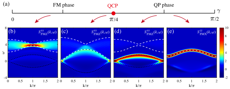
Figure 2: (a) represents a 1D phase diagram of the TFI chain, where a QCP exists at $\gamma_{c}=\pi/4$ separating the FM and QP phases. The nDSF $S^{xx}_{\rm FMZ}(k,\omega)$ results on the direct-product state $\ket{\Phi}_{\rm FMZ}$ along the $\sigma^{z}$ direction are measured (b) in the FM phase ($\gamma=\pi/8$), (c) at QCP ($\gamma=\pi/4$), and (d) in the QP phase ($\gamma=3\pi/8$). The boundaries of two-spinon continua, determined from the exact spinon dispersion in the thermodynamic limit (see Appendix Sec. B), are labeled by white dashed lines, and those of spinon-antispinon continua as black dotted lines. The boundaries agree with our finite size calculations, up to the frequency resolution of the spectral data. (e) is the longitudinal nDSF $S^{zz}_{\rm FMX}(k,\omega)$ measured on the polarized state $\ket{\Phi}_{\rm FMX}$ along the $\sigma^{x}$ direction, with the parameter $\gamma=3\pi/8$ in the Hamiltonian. The analytical dispersion of magnon is labeled by white dashed line, also in excellent agreement with the numerical results.

II Model and Methods

Below we consider the TFI chain, a fundamental lattice model exhibiting fractional spinon excitations and quantum criticality driven by the transverse fields. The Hamiltonian of the TFI model reads,

$$H_{\rm TFI}=-\cos{\gamma}\sum_{i}\sigma_{i}^{z}\sigma_{i+1}^{z}-\sin{\gamma}\sum_{i}\sigma_{i}^{x},$$ (1)

where $\sigma^{\alpha}$’s are Pauli matrices and the parameter $\gamma$ controls the ration between the spin-spin couplings and transverse fields, and a QCP resides at exactly $\gamma_{c}=\pi/4$ [c.f., Fig. 2(a)] that separates the ferromagnetic (FM) phase ($0\leq\gamma<\pi/4$) and quantum paramagnetic (QP) phase ($\pi/4<\gamma\leq\pi/2$). The TFI model can be realized via Rydberg atoms [32, 33, 30] and therefore our many-body studies here also provide useful guide for observing the intriguing dynamical signatures of fractional spinon excitations in quantum simulations.

In the present study, we use the tensor network (TN) based real-time evolution approach [34, 35, 36, 37] to compute the time-dependent spin correlations (see Appendix Sec. A) and also the nDSFs. The key quantity computed with time-dependent TN method here — and proposed to be measured in quantum simulations — reads

$${S^{\alpha\beta}(i,j,t_{1},t_{2})}\equiv \left\langle\sigma_{i}^{\alpha}(t_{1})\sigma_{j}^{\beta}(t_{2})\right\rangle$$ (2)

$$= \left\langle\Phi\right|e^{{\rm i}Ht_{1}}\sigma_{i}^{\alpha}e^{-{\rm i}H(t_{1}-t_{2})}\sigma_{j}^{\beta}e^{-{\rm i}Ht_{2}}\ket{\Phi},$$

where $\ket{\Phi}$ is an initial state hereafter chosen as a direct product state. Below we start from such easy-to-prepare state $\ket{\Phi}$ and compute the real-time evolution after quantum quenches, restricted to the case with $t_{2}=0$ that is also quite natural to measure in quantum simulations.

To be specific, as the time-dependent spin-spin correlation $S^{\alpha\beta}(i,j,t_{1},t_{2}=0)$ is a function of $t(\equiv t_{1})$, we can then compute the nDSF

$$S^{\alpha\beta}(k,\omega)=\frac{1}{L}\sum_{i,j}e^{-{\rm i}k(i-j)}\int_{-\infty}^{\infty}e^{{\rm i}\omega t}{S^{\alpha\beta}(i,j,t)}\,{\rm d}t$$ (3)

to characterize the quenched spin dynamics on the initial state $\ket{\Phi}$ that is in general not the ground state or even eigenstates. We find below the nDSF in Eq. (3) can be used to extract fingerprint information of the spin excitations and are thus the major quantities of interest in the present work.

In the practical calculations, we use the time evolution block decimation approach [34, 35, 36] equipped with the folding trick [38] to evolve the MPO representations of the $\sigma^{\alpha}$ operators from both sides (i.e., in the Heisenberg picture, see details in Appendix Sec. A)). The bond inversion symmetry and time reversal symmetry are employed to reduce computational costs and accelerate the simulations. The bond dimension used in the calculations is $D=800$, which results in a relative truncation error $\lesssim 10^{-5}$ at the maximal evolution time $t_{\textrm{M}}=12$. In order to improve the frequency resolution in computed nDSF, the linear prediction technique [39, 37] has been exploited to extrapolate the time-dependent correlation functions from $t_{\textrm{M}}=12$ to $t_{\textrm{M}}=18$. As $t_{\textrm{M}}$ is still rather limited, we employ the Parzen window function in the time-directional Fourier’s transformation and relieve the artificial oscillations, which results in a frequency resolution with a standard error $\sigma_{\omega}=\sqrt{3}/9$.

III Results

III.1 Multi-Spinon Continua in nDSF

In Fig. 2, we show our results of the nDSF $S(k,\omega)$ computed on different direct product states, which clearly show excitation continua that can be used to detect the fractional spinon excitations. To be specific, we consider below the nDSF $S^{xx}_{\rm FMZ}(k,\omega)$ of $\sigma^{x}$ operators measured in the FM state $\ket{\Phi}_{\rm{FMZ}}\equiv\ket{\uparrow\uparrow...\uparrow}_{z}$ along the $\sigma^{z}$ direction, and $S^{zz}_{\rm FMX}(k,\omega)$ on the product state $\ket{\Phi}_{\rm{FMX}}\equiv\ket{\rightarrow\rightarrow...\rightarrow}_{x}$ along the $\sigma^{x}$ direction, respectively. Intriguingly, from the nDSF results in Fig. 2(b-d) we find excitation continua of the bowtie and shell-like shapes, which represent the two-spinon creation/annihilation and spinon-antispinon processes (c.f., Fig. 1), respectively.

For example, in Fig. 2(b) we see a clear bowtie excitation regime centered at a finite frequency, which represents the two-spinon continuum described by $\omega_{\rm bw}(k)=\epsilon(k_{1})+\epsilon(k_{2})$, with $k=k_{1}+k_{2}$ and $\epsilon(k)=2\sqrt{1-\sin(2\gamma)\cos k}$ (See derivation of the spinon dispersion in Appendix Sec. B and more discussions on the bowtie excitations in Appendix Sec. C). Such two-spinon creation process is illustrated in Fig. 1(c) with the corresponding bowtie continuum illustrated in Fig. 1(a). Moreover, in Fig. 2(b) we depict such upper and lower boundaries of $\omega_{\rm bw}(k)$ and find they bound very well the spinon continuum computed from the product state $\ket{\Phi}_{\rm{FMZ}}$, confirming that these excitation continua in nDSF indeed represent the two-spinon excitations.

The spin flip process can not only create a pair of spinons — the bowtie excitations — but also introduce a spinon-antispinon process [c.f., Fig. 1(d)], as the initial state is not the ground state and can inherently contain spinon excitations already. It thus allows a spinon-antispinon process by a spin flip, and generates a shell-like excitation continua $\omega_{\rm sh}(k)=\epsilon(k_{1})-\epsilon(k_{2})$, with the same single-spinon dispersion $\epsilon(k)$ used in deriving the bowtie excitations. In Fig. 2, we observe that the shell-like shape is rather faint in the FM phase in panel (b), as $\ket{\Phi}_{\rm{FMZ}}$ is rather close to the true ground state and there is no much spectral weight for such spinon-antispinon process. However, the shell-like excitations become very prominent in the QP phase with $\gamma>\gamma_{c}$ [c.f., Fig. 2(d)], where the product state $\ket{\Phi}_{\rm{FMZ}}$ is now far from the ground state and thus the spin flip process can annihilate a spinon and create another [c.f., Fig 1(d)]. At the same time, in Fig. 2(d) the two-spinon creation bowtie excitation continuum becomes virtually invisible. Interestingly, such a role swap of different multi-spinon processes in the prominent excitation continua features between Fig. 2(b) and (d) reflects the existence of a quantum phase transition controlled by the parameter $\gamma$.

Moreover, right at the QCP there emerge features in the system in sharp distinction from both gapped FM and QP phases. At $\gamma_{c}=\pi/4$, the spinon dispersion is $\epsilon(k)=2\sqrt{2}\left|\sin\left(\frac{k}{2}\right)\right|$, which thus leads to $2\sqrt{2}\left|\sin\left(\frac{k}{2}\right)\right|\leq\omega(k)\equiv\epsilon(k_{1})+\epsilon(k_{2})\leq 4\sqrt{2}\left|\sin\left(\frac{k}{4}\right)\right|$ for $\pi<k<2\pi$, and symmetrically for $0<k<\pi$ around $k=\pi$. Besides, we have also plotted the upper and lower boundaries for the spin-antispinon shell regime, i.e., $\pm 2\sqrt{2}\left|\sin\left(\frac{k}{2}\right)\right|$. Note that the upper boundary of spin-antispinon excitation coincides with the lower boundary of the two-spinon creation continuum (see Fig. 1 and also Appendix Sec. C).

In Fig. 1, we have also illustrated the “negative" two-spinon continua corresponding to the annihilation process. Such bowtie excitations with negative energies are not clearly seen in Fig. 2 as the trial state $\ket{\Phi}$ is not “far enough" from the ground state. In the Appendix Sec. C.3 we have provided an example where $\ket{\Phi}$ constitutes a very high energy state and such negative bowtie can be clearly observed there.

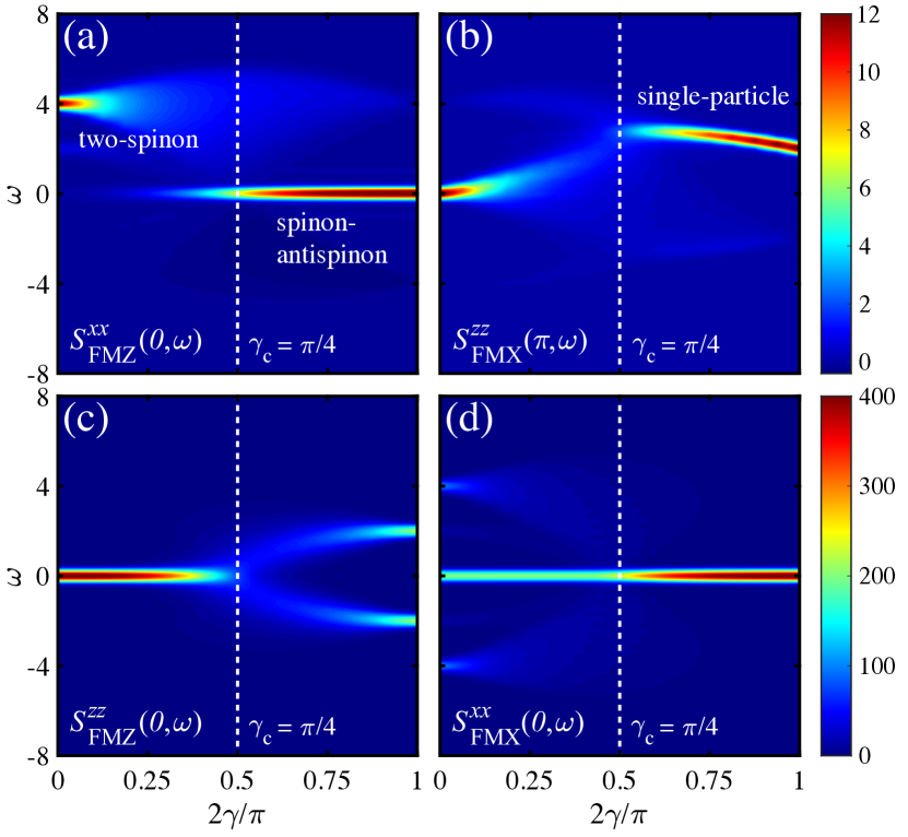
Figure 3: The nDSF results computed on different direct product states $\ket{\Phi}$, scanned vs. various $\gamma$ values. (a, c) show the $k$-cut of $S^{xx}_{\rm FMZ}(k,\omega)$ and $S^{zz}_{\rm FMZ}(k,\omega)$ computed on $\ket{\Phi}_{\rm FMZ}$ state and (b, d) are the two nDSF results measured on the $\ket{\Phi}_{\rm FMX}$ state.

III.2 Lehmann’s Spectral Representation of the nDSF

The results in Fig. 2 show that the nDSF measured on $\ket{\Phi}$ can reflect the multi-spinon continua quantitatively, and besides provide unique access to the spinon-antispinon process that was not accessible in the conventional equilibrium DSF measured on the ground state. To understand that, we employ the Lehmann’s representation of the nDSF and show that the continua there indeed can be associated with the spinon excitations. By inserting the energy eigenstates $\ket{m}$ and $\ket{n}$ in $S^{\alpha\beta}(k,\omega)$ Eq. (3), we find

$$S^{\alpha\beta}(k,\omega)=2\pi\sum_{m,n}\langle\Psi|m\rangle\langle m|\sigma_{k}^{\alpha}|n\rangle\langle n|\sigma_{-k}^{\beta}|\Psi\rangle\,\delta(\omega-\omega_{nm})$$ (4)

where $\sigma_{k}^{\alpha}\equiv\frac{1}{\sqrt{L}}\sum_{j}e^{-{\rm i}kj}\sigma_{j}^{\alpha}$. With this representation Eq. (4), we can now understand the peak position $\omega=\omega_{mn}$ in the nDSF — pole in the Green’s function — indeed represents the intrinsic excitation of the system, as $\omega_{nm}\equiv E_{n}-E_{m}$ is the energy difference between the eigenstates $\ket{m}$ and $\ket{n}$ of the system. Therefore, different from the ground state equilibrium DSF where the excitation energy $\omega$ are positive semi-definite, here $\omega_{mn}$ can be both positive and negative, containing both spinon creation and annihilation processes that lead to the bowtie and shell continua in Figs. 1,2.

With this spectral representation Eq. (4), the excitation continua and distinct dispersions in the nDSF can be understood in a generic sense. For instance, in Fig. 2(e) we show the nDSF $S^{zz}_{\rm FMX}(k,\omega)$ where the initial state $\ket{\Phi}_{\rm FMX}$ is very close to the nearly polarized state induced by the large transverse field, and the nDSF clearly reflects the single-particle dispersion $\epsilon(k)=2\sqrt{1-\sin(2\gamma)\cos k}$.

III.3 Detecting the QCP via the nDSF

As mentioned above, the nDSF results show distinct features in the FM and QP phases in Fig. 2, naturally it suggests that the nDSF can be used to accurately locate the QCP.

In Fig. 3(a) we show the nDSF $S^{xx}_{\rm FMZ}(k=0,\omega)$ which reflects the prominent two-spinon continua in the FM phase [c.f., Fig. 2(a), cut at $k=0$], which changes to the spinon-antispinon feature [Fig. 2(d), also cut at $k=0$] in the QP phase with $\gamma>\gamma_{c}$. To be specific, the behaviors of $S^{xx}_{\rm FMZ}(k=0,\omega)$ change abruptly as $\gamma$ exceeds the critical value of $\gamma_{c}=\pi/4$. The excitation continua get significantly weaker and fide out in the QP phase, and instead there arise a strong intensity at $\omega=0$ which can be ascribed to the shell excitation cut at $k=0$ [c.f., Fig. 2(d)]. Such a transition of excitation behaviors is also reflected in $S^{zz}_{\rm FMX}(k=\pi,\omega)$ in Fig. 3(b), where the single-particle excitation distinct in the QP phase smears out and eventually softens to an excitation energy of $\omega=0$ in the $\gamma=0$ Ising limit.

In Fig. 3(c) we further show $S^{zz}_{\rm FMZ}(k=0,\omega)$ that hosts a clear static peak in the $\gamma=0$ limit. Such peak gradually smears out and becomes branched for $\gamma>\gamma_{c}$, and the splitting that represents the excitation energy $\omega=\omega_{mn}$ equals the eigenvalue differences $\pm 2$ in the $\gamma=\pi/2$ limit. Similarly, in Fig. 3(d) the static peak in $S^{xx}_{\rm FMX}(k=0,\omega)$ at $\omega=0$ in the $\gamma>\gamma_{c}$ side splits into three branches in the FM phase with $\gamma<\gamma_{c}$, forming a triad-like shape. According to the results in Fig. 3, we find that, although the quantum simulator is not initially set at the ground state of the system, the dynamical information in the nDSF nevertheless can be used to detect the QCP with a clear resolution.

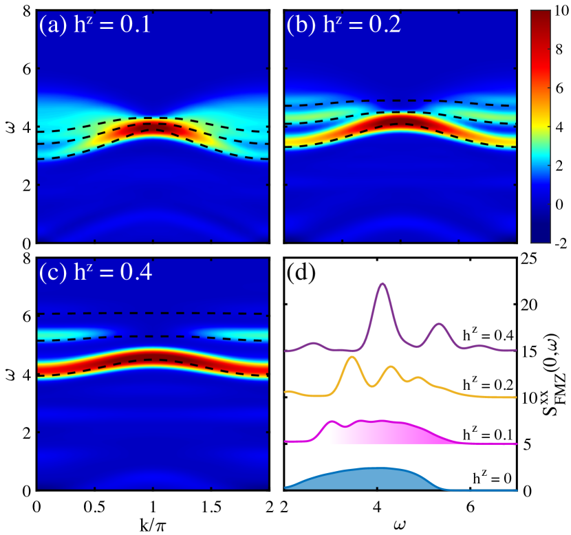
Figure 4: (a-c) show the nDSF $S^{xx}_{\rm FMZ}(k,\omega)$ of the TFI chian in the FM phase ($\gamma=\pi/8$) under longitudinal fields $h^{z}=0.1,0.2,0.4$, where the spinon bound states and the asymptotically free spinons at higher energies, especially when $h^{z}$ is small, can be clearly identified. The dispersions of the spinon bound states agree very well with the perturbative calculations (see Appendix Sec. D), as labeled by the black dashed lines. (d) gives the $k$-cut of (a-c) at the $\Gamma$ point of $k=0$, the two-spinon continuum of the same $\gamma$ while under a zero longitudinal field is also shown as a benchmark. The blue shadow regime in (d) represents the spinon continuum, while the pink regime at $h^{z}=0.1$ reflects asymptotically free spinons alongside with the low-energy peaks of spinon bound states. The lines under finite $h^{z}$ fields in panel (d) are each shifted by a constant of $\Delta\omega=5$ for the sake of clarity.

III.4 Bound States and Asymptotically Free Spinons

When external longitudinal fields are applied additionally, the spinons get confined and form spinon bound states. Recall that a spinon corresponds a domain wall in the FM phase of TFI model, and therefore between two spinons there exists a domain of an opposite spin orientation. Such a 1D domain, string-like object, will pose string tension between two spinons in the presence of a finite longitudinal field. As the confining potential is linear versus the string length $n$ [size of the domain, see Fig. 1(e)], i.e., $V(n)\sim{2}h^{z}\,n$, it introduces a linear attractive interaction between a pair of spinons. The spinon continua at $h^{z}=0$ thus split to several leaves with clear lineshapes, which correspond to the spinon bound states with different length $n$ and can be distinguished clearly in the nDSF $S^{xx}_{\rm FMZ}(k,\omega)$ in Fig. 4(a-c). A perturbative calculation reveals that each of them corresponds to a bound state with distance $n$ (here up to $n=3$) between two constituent spinons (see Appendix Sec. D). Moreover, when the excitation energy becomes high enough, the spinons become very dense and close to each other in real space, thus the effective attraction $V(n)$ gradually becomes irrelevant. Such asymptotically free spinons are evident in the small field $h^{z}=0.1$ case, where excitation continuum is still present in the higher energy regime, as clearly depicted in Fig. 4(d).

III.5 Realization of Dynamical Quantum Simulation with Rydberg Atoms

The proposed phenomena can be observed on contemporary quantum simulation platforms, for instance the Rydberg lattice gases based on arrays of optical tweezers [33, 30, 40], where each qubit is defined on the atomic ground state $\ket{0}$ and one selected Rydberg state $\ket{1}$. The lattice constant can be adjusted properly such that the intra-atom coupling mediated by the van der Waals interactions between Rydberg atoms together with the Rabi coupling and frequency detuning can be well approximated as a quantum Ising model with independently tunable transverse fields and longitudinal fields

$$H_{I}\equiv V\sum_{i}\sigma_{i}^{z}\sigma_{i+1}^{z}+\Omega\sum_{i}\sigma_{i}^{x}+\sum_{i}\Delta_{i}\sigma_{i}^{z}.$$ (5)

The many-body system is initialized as $\ket{\Psi_{0}}\equiv\underset{i=1}{\bigotimes}\ket{0}_{i}$. Then the essential step for the experimental implementation being the measurement of Eq. 2 can be achieved by applying a sequence of gates/operations to the qubits followed by a projective measurement of all qubits in the $\{\ket{0},\ket{1}\}$ basis.

The sequence of gates/operations are composed of $U,e^{-{\rm i}Ht_{2}},\sigma_{j}^{\beta},e^{-{\rm i}H(t_{1}-t_{2})},\sigma_{i}^{\alpha},e^{{\rm i}Ht_{1}}$ and $U^{\dagger}$, where the local unitary operation $U$ rotates the initial state $\ket{\Psi_{0}}$ to a given product state $\ket{\Phi}$ in Eq. (2). Thus, after applying them sequentially to the system one obtains a state

$$\ket{\Psi}=U^{\dagger}e^{{\rm i}Ht_{1}}\sigma_{i}^{\alpha}e^{-{\rm i}H(t_{1}-t_{2})}\sigma_{j}^{\beta}e^{-{\rm i}Ht_{2}}U\ket{\Psi_{0}}.$$ (6)

One can immediately realize that the overlap between $\ket{\Psi}$ and $\ket{\Psi_{0}}$ exactly yields the unequal-time correlation in Eq. 2. In order to implement the operation $e^{{\rm i}Ht_{1}}$, although it is difficult to directly reverse the sign of the system Hamiltonian due to the sign of the interaction, one can effectively realize the whole unitary operation by sandwiching a revised Hamiltonian $H^{\prime}$ with $\sigma^{x}$ operations on the odd sites, i.e., $\Big{(}\underset{i\in odd}{\bigotimes}\sigma_{i}^{x}\Big{)}H^{\prime}\Big{(}\underset{i\in odd}{\bigotimes}\sigma_{i}^{x}\Big{)}$, where $H^{\prime}$ is related to $H_{I}$ as

$$H^{\prime}=V\sum_{i}\sigma_{i}^{z}\sigma_{i+1}^{z}-\Omega\sum_{i}\sigma_{i}^{x}-\sum_{i\in even}\Delta_{i}\sigma_{i}^{z}+\sum_{i\in odd}\Delta_{i}\sigma_{i}^{z}.$$ (7)

One can show by Taylor expansion that

$$e^{{\rm i}H_{I}t}=\Big{(}\underset{i\in odd}{\bigotimes}\sigma_{i}^{x}\Big{)}e^{-{\rm i}H^{\prime}t}\Big{(}\underset{i\in odd}{\bigotimes}\sigma_{i}^{x}\Big{)},$$ (8)

where the r.h.s. is experimentally implementable.

IV Discussion and Outlook

Overall, in this work we explored the non-equlibirum DSF measured on the available states in contemporary quantum simulators. We find, based on the calculations on a prototypical quantum Ising model system, the spin fractionalization can be observed by measuring the nDSF on the direct product states and alike. We show, with solid numerical evidence, that nDSF can be employed to detect the deconfined spinons and their rich creation/annihilation processes not accessible in solid-state experiments, as well as bounded and asymptotically free spinons under finite longitudinal fields. Moreover, the QCP can be identified with the nDSF, even without preparing the delicate ground state.

With this we advocate that these nDSF results have rich connections with the quantum simulation experiments. In distinct to previous proposals of dynamical quantum simulations [41], here we do not require the simulation to start from the ground state or thermal Gibbs state of the Hamiltonian, but from direct product states that are readily accessible in quantum simulators. Such dynamical quantum simulations can offer valuable insight into the quantum many-body systems of interest.

Appendix
“Detecting Confined and Deconfined Spinons in Dynamical Quantum Simulations"

Appendix A Tensor Network Approach for the Dynamical Calculations

Here we provide details of our tensor network algorithm for the calculations of the time-dependent correlation functions

$$S^{\alpha\alpha}(i,j,t_{1},t_{2}=0)=\left\langle\Psi\right|e^{{\rm i}Ht_{1}}\sigma_{i}^{\alpha}e^{-{\rm i}Ht_{1}}\sigma_{j}^{\alpha}\left|\Psi\right\rangle,$$ (9)

where $\alpha=x\text{ or }z$ denotes the two types of spin correlation functions involved in this work.

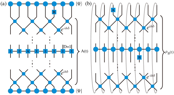
Figure A1: Two schemes to contract the tensor network and compute the time-dependent correlation function $\left\langle\Psi\right|e^{{\rm i}Ht}Ae^{-{\rm i}Ht}B\left|\Psi\right\rangle$. (a) follows the Heisenberg picture and (b) the Schrödinger picture. In both cases, we use TEBD technique to evolve and truncate the MPO.

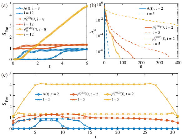
Figure A2: (a) shows the entanglement entropy $S_{\rm Ent}$ versus real time $t$ of the TFI chain at QCP with $L=32$, measured at the $i$-th bond. Operator $\sigma_{8}^{z}$ is chosen in Heisenberg picture, and quenched ground state and FM state along the $\sigma^{z}$ direction are chosen in Schrödinger picture. The entanglement spectra of the $12$-th bond and the spatial distribution of entanglement entropy at $t=2,5$ are shown in (b) and (c), respectively.

A.1 Time Evolution of Matrix Product Operators

Suppose $A$ and $B$ are two local operators (in practice $\sigma_{i}^{\alpha}$ with $\alpha=x,z$), and we would like to calculate the correlation

$$\left\langle\Psi\right|e^{{\rm i}Ht}Ae^{-{\rm i}Ht}B\left|\Psi\right\rangle.$$

To compute it, we can choose to work in the Heisenberg or Schrödinger picture: In the Heisenberg picture, we firstly represent $A$ as a matrix product operator (MPO) with bond dimension $D=1$ because of the locality of the operator. Then, we use the time evolution block decimation (TEBD) approach [34, 35, 36] equipped with the folding trick [38] to evolve the MPO in real time. The time evolution operators $e^{\pm{\rm i}Ht}$ are decomposed via the Trotter-Suzuki decomposition with a Trotter step of $\delta\leq 0.1$ resulting in negligible Trotter error. After obtaining the MPO form of $A(t)\equiv e^{{\rm i}Ht}Ae^{-{\rm i}Ht}$, we contract the tensor network shown in Fig. A1(a) and compute the results of the correlation function.

On the other hand, in Schrödinger picture we instead calculate the time evolution of the density operators (i.e., folded states). The (quenched) density operator is

$$\rho_{B}\equiv B\left|\Psi\right\rangle\left\langle\Psi\right|,$$

and we have

$$\left\langle\Psi\right|e^{{\rm i}Ht}Ae^{-{\rm i}Ht}B\left|\Psi\right\rangle=\mathrm{Tr}\left\{e^{-{\rm i}Ht}\rho_{B}e^{{\rm i}Ht}A\right\}.$$ (10)

As shown in Fig. A1(b), to compute the correlation function we firstly represent $\rho_{B}$ as an MPO with bond dimension $D=1$, and then evolve it from both sides until the whole tensor network is contracted.

The entanglement in either $A(t)$ or $\rho_{B}(t)$ grows rapidly with time, hence we can only simulate relatively short real time with high accuracy. In Fig. A2 we present a comparison between various schemes, where the MPO bond dimension is selected as $D=400$. From the numerical results we find, at least for TFI chains, the Heisenberg picture works better, as the accumulated entanglement is significantly smaller and thus allows for a longer time evolution. Moreover, when working in the Schrödinger picture, one needs to compute $\rho_{B}(t)$ multiple times for different initial states $|\Phi\rangle$, which is highly time consuming as compared to the Heisenberg picture calculations with $A(t)$. Lastly, for operator $\sigma^{x}$, the MPO form of $\sigma_{i}^{x}(t)$ in the TFI chain has a rather compact representation with bond dimension $D=4$. As such, we choose the Heisenberg picture exclusively.

For the calculations in the main text, we eventually choose $D=800$ and perform the simulations to a time period of $t_{M}=12$, with truncation error $\lesssim 10^{-5}$.

A.2 Bond Inversion and Time Reversal Symmetries

Note that both the TFI Hamiltonian in Eq. (1) of the main text, even with longitudinal external fields, as well as the density operators $\rho$ we consider in the present work have a $\mathbb{Z}_{2}^{2}$ symmetry, with the two 2-nd ordered generators, i.e. bond-inversion $\mathcal{B}$ and the generalized time reversal $\mathcal{O}\equiv\mathcal{R}_{y}\mathcal{T}$, where $\mathcal{R}_{y}$ is the $\pi$-rotation along the $\sigma^{y}$ direction and $\mathcal{T}$ represents the time reversal. Assuming an even length $L$, we have the following two equations that can be exploited to accelerate our time-dependent calculations.

$$\left\{\begin{aligned} &S^{\alpha\alpha}(L-i+1,L-j+1,t)=S^{\alpha\alpha}(i,j,t)\\ &S^{\alpha\alpha}(i,j,-t)=\overline{S^{\alpha\alpha}(i,j,t)}\end{aligned}\right.$$ (11)

With these relations, we can save the computational costs in the sense that only about one quarter of correlation functions are needed to be computed, which greatly facilitates the calculations.

The first equation follows the bond inversion symmetry, and we provide a brief proof of the second equation. Firstly,

$$S^{\alpha\alpha}(i,j,-t)= \mathrm{Tr}\left\{\rho e^{-{\rm i}Ht}\sigma_{i}^{\alpha}e^{{\rm i}Ht}\sigma_{j}^{\alpha}\right\}$$ (12)

$$= \mathrm{Tr}\left\{\mathcal{O}\rho e^{{\rm i}Ht}\mathcal{O}\sigma_{i}^{\alpha}\mathcal{O}e^{-{\rm i}Ht}\mathcal{O}\sigma_{j}^{\alpha}\mathcal{O}^{2}\right\},$$

where $\mathcal{O}\rho\mathcal{O}=\rho$ and $\mathcal{O}e^{\pm{\rm i}Ht}\mathcal{O}=e^{\mp{\rm i}Ht}$ are used. Considering $\mathcal{O}\sigma^{x}\mathcal{O}=\sigma^{x}$, $\mathcal{O}\sigma^{y}\mathcal{O}=-\sigma^{y}$, $\mathcal{O}\sigma^{z}\mathcal{O}=\sigma^{z}$, no matter $\alpha=x,y$ or $z$, we always have

$${\rm R.H.S.}=\mathrm{Tr}\left\{\mathcal{O}\rho e^{{\rm i}Ht}\sigma_{i}^{\alpha}e^{-{\rm i}Ht}\sigma_{j}^{\alpha}\mathcal{O}\right\}.$$ (13)

Note that $\mathcal{O}$ is anti-linear so that $\mathrm{Tr}\left\{\mathcal{O}\cdots\mathcal{O}\right\}=\overline{\mathrm{Tr}\left\{\cdots\right\}}$, finally

$$S^{\alpha\alpha}(i,j,-t)=\overline{\mathrm{Tr}\left\{\rho e^{{\rm i}Ht}\sigma_{i}^{\alpha}e^{-{\rm i}Ht}\sigma_{j}^{\alpha}\right\}}=\overline{S^{\alpha\alpha}(i,j,t)}.$$ (14)

Worth to point out, although Neél state along the $\sigma^{z}$ direction is not invariant under either $\mathcal{B}$ or $\mathcal{R}_{y}\mathcal{T}$, it is invariant under $\mathcal{R}_{x}\mathcal{B}$ and $\mathcal{R}_{x}\mathcal{T}$. Thanks to such symmetry, we can also accelerate the calculations in such case.

A.3 3. Window Functions in Fourier’s Transformation

Now we consider the Fourier’s transformation (FT) from time space to frequency space, i.e.,

$$\mathcal{F}[f(t)](\omega)\equiv\int_{-\infty}^{\infty}{\rm d}te^{{\rm i}\omega t}f(t),$$ (15)

which can be computed with the numerical integral. In the tensor network calculations, we have only access to a finite time $t$ window, i.e., $t\in[-t_{M},t_{M}]$. Hence, we adopt the Parzen function, a Gauss-like window function but with compact support,

$$W(x;a)=\left\{\begin{aligned} &1-6\left|\frac{x}{a}\right|^{2}+6\left|\frac{x}{a}\right|^{3},\ &|x|\leq\frac{a}{2}\\ &2\left(1-\left|\frac{x}{a}\right|\right)^{3},\ &\frac{a}{2}<|x|\leq a\\ &0,\ &|x|>a\end{aligned}\right.$$ (16)

and multiply it to the time-dependent correlation functions in order to suppress the non-physical oscillating due to time truncation [42]. Hence, we actually calculate

$$\int_{-t_{M}}^{t_{M}}{\rm d}te^{{\rm i}\omega t}f(t)W(t;t_{M})$$ (17)

$$= \int_{-\infty}^{\infty}{\rm d}te^{{\rm i}\omega t}f(t)W(t;t_{M})$$

$$= \frac{1}{2\pi}\int_{-\infty}^{\infty}{\rm d}\omega^{\prime}\mathcal{F}[f(t)](\omega^{\prime})\mathcal{F}[W(t;t_{M})](\omega-\omega^{\prime})$$

$$= \frac{1}{2\pi}\mathcal{F}[f(t)](\omega)\ast\mathcal{F}[W(t;t_{M})](\omega),$$

where the convolution kernel is

$$\frac{1}{2\pi}\mathcal{F}[W(t;t_{M})]=\frac{96\sin^{4}\left(t_{M}\omega/4\right)}{\pi t_{M}^{4}\omega^{4}},$$ (18)

whose standard error in frequency space is $2\sqrt{3}/t_{M}$, characterizing the frequency resolution.

A.4 Linear Prediction Techniques in the Dynamical Calculations

Linear prediction is a commonly used method to improve the energy resolution in dynamical properties [39, 37]. Its key point is use the linear combination of the data we have to predict the regime we do not have access. Consider a series $\{x_{i}\}$, $k$-order linear prediction gives

$$\hat{x}_{n}=\sum_{i=1}^{k}a_{i}x_{n-i},$$ (19)

where the coefficients $a_{i}$ are determined by fitting the known data. There are many different fitting algorithms to calculate the coefficients, e.g., Burg’s method [43] adopted in the present work. With this, we can predict the correlation function with $t>t_{M}$, which can significantly improve the frequency resolution.

We call a series line spectral, if the FT of it is a summation of a few Dirac $\delta$-functions, and the general theory of linear prediction guarantees that when the results are closer to a line spectral series, the linear prediction will work better and provide more accurate results[44]. Due to this consideration, we apply linear prediction to the time-dependent correlation functions in momentum space

$$S^{\alpha\beta}(k,t)\equiv\frac{1}{L}\sum_{i,j}e^{-{\rm i}k(i-j)}S^{\alpha\beta}(i,j,t).$$ (20)

Fig. A3(f) shows the benchmark results on the nDSF $S_{\rm FMX}^{zz}(k=\pi,\omega)$, which reflects the magnon excitation in the QP phase and is standardly line spectral up to finite size effects. As a result, the linear prediction from $t_{M}=8$ to $t_{M}=12$ works excellently as shown in Fig. A3(b). However, compared to that in momentum space, the linear prediction of real-space correlations like $S^{zz}(i,j,t)$ results in a visible error as seen in Fig. A3(a). Therefore, it suggests us to work in momentum space. For the spectrum with spinon continua, e.g., the correlation $S_{\rm FMZ}^{xx}(k=\pi,\omega)$ $k$-cut at $k=\pi$ in Fig. 2(d) of the main text, the linear prediction does not works well in both real and momentum spaces, c.f., Fig. A3(c,d). Nevertheless, the obtained spectral functions still coincide with the exact results, as shown in Fig. A3(g,h), which may be due to the fact that window function makes the finite value of $t\to t_{M}$ less important. By these trial calculations, we think that our spectra calculated after linear prediction in the main text are reliable.

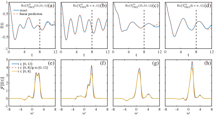
Figure A3: Panels (a-d) show the benchmarks of the linear prediction from $t\in[0,8]$ to $t\in[0,12]$ versus the numerically exact results. We show the time-dependent correlation in the QP phase ($\gamma=3\pi/8)$, measured (a) on the FMX state and (c) on the FMZ state. (b,d) are the counterparts of (a,c) after a spatial FT, and the lower panels (e-h) show the FT in frequency space of the time-dependent correlation functions in (a-d).

Appendix B Free Fermion Representation of TFI Chain

Hamiltonian (1) can be transformed to free fermion representation via Jordan-Wigner transformation. Here our convention is

$$\left\{\begin{aligned} &\sigma_{i}^{x}=2c_{i}^{\dagger}c_{i}-1\\ &\sigma_{i}^{y}=K_{i}(c_{i}+c_{i}^{\dagger})\\ &\sigma_{i}^{z}=iK_{i}(c_{i}-c_{i}^{\dagger})\\ \end{aligned}\right.$$ (21)

where

$$K_{i}=\prod_{j=1}^{i-1}\sigma_{j}^{x}=\prod_{j=1}^{i-1}(2c_{j}^{\dagger}c_{j}-1)$$ (22)

represents the Jordan-Wigner string. Using $\{\sigma_{i}^{y}\pm i\sigma_{i}^{z},\sigma_{i}^{x}\}=0$, one can check the fermion relationship

$$\{c_{i},c_{j}^{\dagger}\}=\delta_{ij},\ \{c_{i},c_{j}\}=\{c_{i}^{\dagger},c_{j}^{\dagger}\}=0.$$ (23)

Then, the free fermion Hamiltonian of TFI chain is

$$H= -\cos\gamma\sum_{i}\left(c_{i}^{\dagger}+c_{i}\right)\left(c_{i+1}^{\dagger}-c_{i+1}\right)$$ (24)

$$-\sin\gamma\sum_{i}\left(c_{i}^{\dagger}c_{i}-c_{i}c_{i}^{\dagger}\right).$$

Here we assume the periodic boundary condition for the free fermion Hamiltonian, which does not alter the physics in the thermodynamic limit $L\to\infty$. Then, we can apply a spatial FT

$$f_{k}=\frac{1}{\sqrt{L}}\sum_{n}e^{-{\rm i}kn}c_{n},\ k=-\pi,-\pi+\frac{2\pi}{L},\cdots,0,\cdots,\pi-\frac{2\pi}{L}$$ (25)

to get the BdG Hamiltonian

$$H=\sum_{k\geq 0}[f_{k}^{\dagger}\ f_{-k}]\left[\begin{matrix}&2\cos\gamma\cos k-2\sin\gamma&-2i\cos\gamma\sin k\\ &2i\cos\gamma\sin k&-2\cos\gamma\cos k+2\sin\gamma\end{matrix}\right]\left[\begin{matrix}f_{k}\\ f_{-k}^{\dagger}\end{matrix}\right]\equiv\sum_{k\geq 0}\Psi_{k}^{\dagger}\widetilde{H}(k)\Psi_{k}.$$ (26)

Diagonalize $\widetilde{H}(k)=V(k)D(k)V^{\dagger}(k)$, where $D(k)=\mathrm{diag}[\epsilon_{k},-\epsilon_{k}]$, we get

$$H=\sum_{k\geq 0}\epsilon_{k}\left(\eta_{k}^{\dagger}\eta_{k}-\eta_{-k}\eta_{-k}^{\dagger}\right)=\sum_{k}\epsilon_{k}\left(\eta_{k}^{\dagger}\eta_{k}-\frac{1}{2}\right)$$ (27)

with $[\eta_{k}^{\dagger}\ \eta_{-k}]=\Psi_{k}^{\dagger}V(k)$. The dispersion reads

$$\epsilon(k)=2\sqrt{1-\sin(2\gamma)\cos k},$$ (28)

and in the limit of Ising coupling ($\gamma\to 0$) or transverse field ($\gamma\to\pi/2$), it becomes

$$\epsilon(k)\simeq 2-\sin(2\gamma)\cos k.$$ (29)

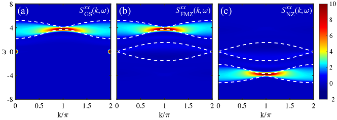
Figure A4: The nDSF $S^{xx}(k,\omega)$ of the TFI model at $\gamma=\pi/8$. (a) is DSF measured on the ground state, where only the two-spinon continuum can be identified, except for the static peak at the $\Gamma$ point due to the finite transverse field. (b) shows the nDSF measured on $\ket{\Phi_{\rm FMZ}}$, where we see both the two-spinon continuum and the weaker spinon-antispinon continuum. (c) presents the nDSF measured on the Neél state along the $\sigma^{z}$ direction, which is a product state far from the ground state. In this case, the two-antispinon continuum can be clearly recognized.

Appendix C The Bowtie and Shell-like Excitations in the nDSF

C.1 Excitation Continua in the Gapped Phases

Here we give a simple derivation of the bowtie and shell-like excitations in nDSF. The bowtie excitations correspond to two-spinon creation, and the shell-like excitations correspond to spinon-antispinon process, as shown in Fig. 1 of the main text. Note that in Fig. 2 of the main text we used the exact dispersion Eq. (28) to calculate the boundaries numerically away from the QCP, but below we will use the approximative dispersion Eq. (29) so that we can obtain analytical results of the boundary. The two-spinon continuum is determined by $k=k_{1}+k_{2}$ and $\omega(k)=\epsilon(k_{1})+\epsilon(k_{2})$. Substitute the dispersion $\epsilon(k)$ in Eq. (29) into $\omega(k)$, we have

$$\omega(k) = 4-\sin(2\gamma)\cos k_{1}-\sin(2\gamma)\cos k_{2}$$ (30)

$$= 4-2\sin(2\gamma)\cos\left(\frac{k}{2}\right)\cos\left(\frac{k_{1}-k_{2}}{2}\right).$$

Then we get the boundary

$$4\pm 2\sin(2\gamma)\left|\cos\left(\frac{k}{2}\right)\right|,$$

where we set $\left|\cos\left(\frac{k_{1}-k_{2}}{2}\right)\right|=1$. For the two-spinon annihilation, note that the dispersion of antispinon is $-\epsilon(k)$, two-antispinon boundary is just

$$-4\pm 2\sin(2\gamma)\left|\cos\left(\frac{k}{2}\right)\right|.$$

Similarly, the spinon-antispinon continuum reads

$$\omega(k)= \epsilon(k_{1})-\epsilon(k_{2})$$ (31)

$$= -\sin(2\gamma)\cos k_{1}+\sin(2\gamma)\cos k_{2}$$

$$= 2\sin(2\gamma)\sin\left(\frac{k}{2}\right)\sin\left(\frac{k_{1}-k_{2}}{2}\right),$$

which gives the symmetric upper and lower boundary

$$\pm 2\sin(2\gamma)\left|\sin\left(\frac{k}{2}\right)\right|.$$

The above bowtie and shell-like excitations are shown in Fig. 1(a) of the main text.

It is worth to mention that when we use the exact dispersion, instead of the cos-type one in the Ising or large-field limits, the upper and lower boundaries of the bowtie excitations are no longer symmetric, and there will be a finite linewidth at $k=\pi$, as shown in Fig. 2(b,d) of the main text, instead of purely a node in Fig. 1(a).

C.2 Excitation Continua at the QCP

Exactly at QCP, the spinon dispersion reads

$$\epsilon(k)=2\sqrt{2}\left|\sin\left(\frac{k}{2}\right)\right|,$$ (32)

and the two-spinon continuum can be written as

$$\omega(k)=\epsilon(k_{1})+\epsilon(k_{2})=\epsilon\left(\frac{k}{2}+\delta\right)+\epsilon\left(\frac{k}{2}-\delta\right).$$ (33)

Firstly we consider the case of $0\leq k<\pi$, then

$$\omega(k)=\left\{\begin{aligned} &4\sqrt{2}\sin\left(\frac{k}{4}\right)\cos\left(\frac{\delta}{2}\right),\ &0\leq\delta<k/2\\ &4\sqrt{2}\cos\left(\frac{k}{4}\right)\sin\left(\frac{\delta}{2}\right),\ &k/2\leq\delta<2\pi-k/2\\ &-4\sqrt{2}\sin\left(\frac{k}{4}\right)\cos\left(\frac{\delta}{2}\right),\ &2\pi-k/2\leq\delta<2\pi\\ \end{aligned}\right.$$ (34)

Considering all these cases, $\omega(k)$ reaches its lower bound $2\sqrt{2}\sin\left(k/2\right)$ at $\delta=k/2$ and its upper bound $4\sqrt{2}\cos\left(k/4\right)$ at $\delta=\pi$. Similarly, in the case of $\pi\leq k<2\pi$, $\omega(k)$ reaches its lower bound $2\sqrt{2}\sin\left(k/2\right)$ at $\delta=k/2$ and its upper bound $4\sqrt{2}\sin\left(k/4\right)$ at $\delta=0$. Also consider the case of $0\leq k<\pi$, the spinon-antispinon continuum can be written as

$$\omega(k)=\epsilon(k_{1})-\epsilon(k_{2})=\epsilon\left(\frac{k}{2}+\delta\right)-\epsilon\left(\frac{k}{2}-\delta\right).$$ (35)

Note that it is an odd function of $\delta$, the boundary of spinon-antispinon continuum is much easier to calculate. Because of the sine-type dispersion (32), $\partial\omega/\partial\delta\geq 0$ holds for all $|\delta|<k/2$ and $\partial\omega/\partial\delta\leq 0$ holds for all $k/2<|\delta|<\pi$. Hence, $\omega(k)$ must reach its bound at $\delta=\pm k/2$ or $\pm\pi$. However, the latter must result in $\omega(k)=0$ because it is both odd and $2\pi$-periodic. Finally, we get its boundary $\pm 2\sqrt{2}\left|\sin\left(k/2\right)\right|$. The bowtie and shell excitations at QCP are illustrated in Fig. 1(b) of the main text.

C.3 Two-Spinon Annihilation Continua

We have shown the two-spinon and spinon-antispinon continua in the nDSF measured on direct product states in the main text. The two-spinon annihilation process can also be seen if we choose states with high energy, i.e., far from the ground state. Fig. A4 shows the nDSF $S^{xx}(k,\omega)$ at $\gamma=\pi/8$ measured on different product states, equilibrium DSF measured on ground state is also shown in panel (a) as a comparison.

Appendix D Dispersion of Spinon Bound States of TFI Chain with Longitudinal Fields

The Hamiltonian of TFI chain under a longitudinal field reads

$$H=-\cos{\gamma}\sum_{i}\sigma_{i}^{z}\sigma_{i+1}^{z}-\sin{\gamma}\sum_{i}\sigma_{i}^{x}-h^{z}\sum_{i}\sigma^{z},$$ (36)

where $h^{z}$ is the strength of the longitudinal field. We consider the FM phase, and take the transverse fields as perturbation in the $\gamma\to 0$ limit. Denote

$$|i;n\rangle\equiv|\uparrow\cdots\uparrow\underbrace{\downarrow_{i}\cdots\downarrow_{i+n-1}}_{n}\uparrow\cdots\rangle$$ (37)

as the state with two spinons, where $i$ is the starting site and $n$ is the length of the domain. We also assume $h^{z}\ll 1$ such that the Ising couplings dominate the Hamiltonian, hence the states with more spinons can be neglected because of the large gap $\Delta\gtrsim 2\cos\gamma$. All such states $\{\ket{i;n}\}$ span a subspace, and we perform the first ordered degenerate perturbation calculations in this subspace. After shifting zero point of energy s.t. $\langle\uparrow\cdots\uparrow|H|\uparrow\cdots\uparrow\rangle=0$ for convenience,

$$H_{\rm eff}|i;n\rangle=\left(4\cos\gamma+2nh^{z}\right)|i;n\rangle-\sin\gamma\left(|i;n+1\rangle+|i;n-1\rangle+|i-1;n+1\rangle+|i+1;n-1\rangle\right).$$ (38)

A given bound state is the state with two spinons carrying the same quasi-momentum, hence $n$ is unchanging. So we apply FT for each fixed $n$

$$|k;n\rangle\equiv\frac{1}{L}\sum_{j}e^{-{\rm i}kj}|j;n\rangle.$$ (39)

Then, in the Fourier basis the effective Hamiltonian is partially decoupled,

$$H_{\rm eff}|k;n\rangle=\left(4\cos\gamma+2nh^{z}\right)|k;n\rangle-\sin\gamma\left(|k;n+1\rangle+|k;n-1\rangle+e^{-ik}|k;n+1\rangle+e^{ik}|k;n-1\rangle\right).$$ (40)

Now we fix $k$ and get the effective Hamiltonian

$$\langle k;m|H_{\rm eff}|k;n\rangle=\left(4\cos\gamma+2nh^{z}\right)\delta_{mn}-\sin\gamma\left(1+e^{-ik}\right)\delta_{m,n+1}-\sin\gamma\left(1+e^{ik}\right)\delta_{m,n-1},$$ (41)

where the position $m,n\geq 1$. We introduce a cutoff $m,n\leq N$, which is quite nature as the spinon confinement induced by $h^{z}$ fields. In this basis, $H_{\rm eff}$ forms a tridiagonial $N\times N$ Hermitian matrix, which can be diagonalized and there are $N$ eigenvalues. Apply this procedure for each $k$ and we get the dispersion of the $N$ spinon bound states.

References

- Giamarchi [2004] T. Giamarchi, Quantum physics in one dimension (Clarendon Press, 2004).
- Lake et al. [2013] B. Lake, D. A. Tennant, J.-S. Caux, T. Barthel, U. Schollwöck, S. E. Nagler, and C. D. Frost, Multispinon continua at zero and finite temperature in a near-ideal Heisenberg chain, Phys. Rev. Lett. 111, 137205 (2013).
- Mourigal et al. [2013] M. Mourigal, M. Enderle, A. Klöpperpieper, J.-S. Caux, A. Stunault, and H. M. Rønnow, Fractional spinon excitations in the quantum Heisenberg antiferromagnetic chain, Nature Physics 9, 435 (2013).
- Wu et al. [2016] L. S. Wu, W. J. Gannon, I. A. Zaliznyak, A. M. Tsvelik, M. Brockmann, J.-S. Caux, M. S. Kim, Y. Qiu, J. R. D. Copley, G. Ehlers, A. Podlesnyak, and M. C. Aronson, Orbital-exchange and fractional quantum number excitations in an f-electron metal, Yb2Pt2Pb, Science 352, 1206 (2016).
- Coldea et al. [2010] R. Coldea, D. A. Tennant, E. M. Wheeler, E. Wawrzynska, D. Prabhakaran, M. Telling, K. Habicht, P. Smeibidl, and K. Kiefer, Quantum criticality in an Ising chain: experimental evidence for emergent E8 symmetry, Science 327, 177 (2010).
- Morris et al. [2014] C. M. Morris, R. Valdés Aguilar, A. Ghosh, S. M. Koohpayeh, J. Krizan, R. J. Cava, O. Tchernyshyov, T. M. McQueen, and N. P. Armitage, Hierarchy of bound states in the one-dimensional ferromagnetic Ising chain investigated by high-resolution time-domain terahertz spectroscopy, Phys. Rev. Lett. 112, 137403 (2014).
- Fava et al. [2020] M. Fava, R. Coldea, and S. A. Parameswaran, Glide symmetry breaking and Ising criticality in the quasi-1D magnet CoNb2O6, Proceedings of the National Academy of Sciences 117, 25219 (2020).
- Morris et al. [2021] C. M. Morris, N. Desai, J. Viirok, D. Hüvonen, U. Nagel, T. Rõõm, J. W. Krizan, R. J. Cava, T. M. McQueen, S. M. Koohpayeh, R. K. Kaul, and N. P. Armitage, Duality and domain wall dynamics in a twisted Kitaev chain, Nature Physics 17, 832 (2021).
- Gannon et al. [2019] W. J. Gannon, I. A. Zaliznyak, L. S. Wu, A. E. Feiguin, A. M. Tsvelik, F. Demmel, Y. Qiu, J. R. D. Copley, M. S. Kim, and M. C. Aronson, Spinon confinement and a sharp longitudinal mode in Yb2Pt2Pb in magnetic fields, Nature Communications 10, 1123 (2019).
- Wu et al. [2019] L. S. Wu, S. E. Nikitin, Z. Wang, W. Zhu, C. D. Batista, A. M. Tsvelik, A. M. Samarakoon, D. A. Tennant, M. Brando, L. Vasylechko, M. Frontzek, A. T. Savici, G. Sala, G. Ehlers, A. D. Christianson, M. D. Lumsden, and A. Podlesnyak, Tomonaga–Luttinger liquid behavior and spinon confinement in YbAlO3, Nature Communications 10, 698 (2019).
- Ladd et al. [2010] T. D. Ladd, F. Jelezko, R. Laflamme, Y. Nakamura, C. Monroe, and J. L. O’Brien, Quantum computers, Nature 464, 45 (2010).
- Georgescu [2020] I. Georgescu, Trapped ion quantum computing turns 25, Nature Reviews Physics 2, 278 (2020).
- Green et al. [2021] D. Green, H. Soller, Y. Oreg, and V. Galitski, How to profit from quantum technology without building quantum computers, Nature Reviews Physics 3, 150 (2021).
- de Leon et al. [2021] N. P. de Leon, K. M. Itoh, D. Kim, K. K. Mehta, T. E. Northup, H. Paik, B. S. Palmer, N. Samarth, S. Sangtawesin, and D. W. Steuerman, Materials challenges and opportunities for quantum computing hardware, Science 372 (2021).
- Georgescu et al. [2014] I. M. Georgescu, S. Ashhab, and F. Nori, Quantum simulation, Rev. Mod. Phys. 86, 153 (2014).
- Kokail et al. [2019] C. Kokail, C. Maier, R. van Bijnen, T. Brydges, M. K. Joshi, P. Jurcevic, C. A. Muschik, P. Silvi, R. Blatt, C. F. Roos, and P. Zoller, Self-verifying variational quantum simulation of lattice models, Nature 569, 355 (2019).
- Keesling et al. [2019] A. Keesling, A. Omran, H. Levine, H. Bernien, H. Pichler, S. Choi, R. Samajdar, S. Schwartz, P. Silvi, S. Sachdev, P. Zoller, M. Endres, M. Greiner, V. Vuletić, and M. D. Lukin, Quantum Kibble–Zurek mechanism and critical dynamics on a programmable Rydberg simulator, Nature 568, 207 (2019).
- Choi et al. [2016] J.-y. Choi, S. Hild, J. Zeiher, P. Schauß, A. Rubio-Abadal, T. Yefsah, V. Khemani, D. A. Huse, I. Bloch, and C. Gross, Exploring the many-body localization transition in two dimensions, Science 352, 1547 (2016).
- Smith et al. [2016] J. Smith, A. Lee, P. Richerme, B. Neyenhuis, P. W. Hess, P. Hauke, M. Heyl, D. A. Huse, and C. Monroe, Many-body localization in a quantum simulator with programmable random disorder, Nature Physics 12, 907 (2016).
- Xu et al. [2018] K. Xu, J.-J. Chen, Y. Zeng, Y.-R. Zhang, C. Song, W. Liu, Q. Guo, P. Zhang, D. Xu, H. Deng, K. Huang, H. Wang, X. Zhu, D. Zheng, and H. Fan, Emulating many-body localization with a superconducting quantum processor, Phys. Rev. Lett. 120, 050507 (2018).
- Guo et al. [2021] Q. Guo, C. Cheng, Z.-H. Sun, Z. Song, H. Li, Z. Wang, W. Ren, H. Dong, D. Zheng, Y.-R. Zhang, R. Mondaini, H. Fan, and H. Wang, Observation of energy-resolved many-body localization, Nature Physics 17, 234 (2021).
- Cheuk et al. [2016a] L. W. Cheuk, M. A. Nichols, K. R. Lawrence, M. Okan, H. Zhang, and M. W. Zwierlein, Observation of 2D fermionic Mott insulators of with single-site resolution, Phys. Rev. Lett. 116, 235301 (2016a).
- Cheuk et al. [2016b] L. W. Cheuk, M. A. Nichols, K. R. Lawrence, M. Okan, H. Zhang, E. Khatami, N. Trivedi, T. Paiva, M. Rigol, and M. W. Zwierlein, Observation of spatial charge and spin correlations in the 2D Fermi-Hubbard model, Science 353, 1260 (2016b).
- Mazurenko et al. [2017] A. Mazurenko, C. S. Chiu, G. Ji, M. F. Parsons, M. Kanász-Nagy, R. Schmidt, F. Grusdt, E. Demler, D. Greif, and M. Greiner, A cold-atom Fermi–Hubbard antiferromagnet, Nature 545, 462 (2017).
- Chiu et al. [2019] C. S. Chiu, G. Ji, A. Bohrdt, M. Xu, M. Knap, E. Demler, F. Grusdt, M. Greiner, and D. Greif, String patterns in the doped Hubbard model, Science 365, 251 (2019).
- Koepsell et al. [2019] J. Koepsell, J. Vijayan, P. Sompet, F. Grusdt, T. A. Hilker, E. Demler, G. Salomon, I. Bloch, and C. Gross, Imaging magnetic polarons in the doped Fermi–Hubbard model, Nature 572, 358 (2019).
- Yan et al. [2019] Z. Yan, Y.-R. Zhang, M. Gong, Y. Wu, Y. Zheng, S. Li, C. Wang, F. Liang, J. Lin, Y. Xu, C. Guo, L. Sun, C.-Z. Peng, K. Xia, H. Deng, H. Rong, J. Q. You, F. Nori, H. Fan, X. Zhu, and J.-W. Pan, Strongly correlated quantum walks with a 12-qubit superconducting processor, Science 364, 753 (2019).
- Gong et al. [2021] M. Gong, S. Wang, C. Zha, M.-C. Chen, H.-L. Huang, Y. Wu, Q. Zhu, Y. Zhao, S. Li, S. Guo, H. Qian, Y. Ye, F. Chen, C. Ying, J. Yu, D. Fan, D. Wu, H. Su, H. Deng, H. Rong, K. Zhang, S. Cao, J. Lin, Y. Xu, L. Sun, C. Guo, N. Li, F. Liang, V. M. Bastidas, K. Nemoto, W. J. Munro, Y.-H. Huo, C.-Y. Lu, C.-Z. Peng, X. Zhu, and J.-W. Pan, Quantum walks on a programmable two-dimensional 62-qubit superconducting processor, Science 372, 948 (2021).
- Browaeys et al. [2016] A. Browaeys, D. Barredo, and T. Lahaye, Experimental investigations of dipole–dipole interactions between a few Rydberg atoms, Journal of Physics B: Atomic, Molecular and Optical Physics 49, 152001 (2016).
- Omran et al. [2019] A. Omran, H. Levine, A. Keesling, G. Semeghini, T. T. Wang, S. Ebadi, H. Bernien, A. S. Zibrov, H. Pichler, S. Choi, J. Cui, M. Rossignolo, P. Rembold, S. Montangero, T. Calarco, M. Endres, M. Greiner, V. Vuletić, and M. D. Lukin, Generation and manipulation of Schrödinger cat states in Rydberg atom arrays, Science 365, 570 (2019).
- Song et al. [2019] C. Song, K. Xu, H. Li, Y.-R. Zhang, X. Zhang, W. Liu, Q. Guo, Z. Wang, W. Ren, J. Hao, H. Feng, H. Fan, D. Zheng, D.-W. Wang, H. Wang, and S.-Y. Zhu, Generation of multicomponent atomic Schrödinger cat states of up to 20 qubits, Science 365, 574 (2019).
- Schauß et al. [2015] P. Schauß, J. Zeiher, T. Fukuhara, S. Hild, M. Cheneau, T. Macrì, T. Pohl, I. Bloch, and C. Gross, Crystallization in Ising quantum magnets, Science 347, 1455 (2015).
- Bernien et al. [2017] H. Bernien, S. Schwartz, A. Keesling, H. Levine, A. Omran, H. Pichler, S. Choi, A. S. Zibrov, M. Endres, M. Greiner, V. Vuletić, and M. D. Lukin, Probing many-body dynamics on a 51-atom quantum simulator, Nature 551, 579 (2017).
- Vidal [2004] G. Vidal, Efficient simulation of one-dimensional quantum many-body systems, Phys. Rev. Lett. 93, 040502 (2004).
- White and Feiguin [2004] S. R. White and A. E. Feiguin, Real-time evolution using the density matrix renormalization group, Phys. Rev. Lett. 93, 076401 (2004).
- Vidal [2007] G. Vidal, Classical simulation of infinite-size quantum lattice systems in one spatial dimension, Phys. Rev. Lett. 98, 070201 (2007).
- Barthel et al. [2009] T. Barthel, U. Schollwock, and S. R. White, Spectral functions in one-dimensional quantum systems at finite temperature using the density matrix renormalization group, Phys. Rev. B 79, 245101 (2009).
- Bañuls et al. [2009] M. C. Bañuls, M. B. Hastings, F. Verstraete, and J. I. Cirac, Matrix product states for dynamical simulation of infinite chains, Phys. Rev. Lett. 102, 240603 (2009).
- White and Affleck [2008] S. R. White and I. Affleck, Spectral function for the Heisenberg antiferromagetic chain, Phys. Rev. B 77, 134437 (2008).
- Ebadi et al. [2021] S. Ebadi, T. T. Wang, H. Levine, A. Keesling, G. Semeghini, A. Omran, D. Bluvstein, R. Samajdar, H. Pichler, W. W. Ho, S. Choi, S. Sachdev, M. Greiner, V. Vuletić, and M. D. Lukin, Quantum phases of matter on a 256-atom programmable quantum simulator, Nature 595, 227 (2021).
- Baez et al. [2020] M. L. Baez, M. Goihl, J. Haferkamp, J. Bermejo-Vega, M. Gluza, and J. Eisert, Dynamical structure factors of dynamical quantum simulators, Proceedings of the National Academy of Sciences 117, 26123 (2020).
- Kühner and White [1999] T. D. Kühner and S. R. White, Dynamical correlation functions using the density matrix renormalization group, Phys. Rev. B 60, 335 (1999).
- Kay [1988] S. Kay, Modern spectral estimation: theory and application, Prentice-Hall signal processing series (Prentice-Hall, 1988).
- Vaidyanathan [2007] P. P. Vaidyanathan, The theory of linear prediction (Morgan & Claypool, 2007).